Balancing Communication and Computation in Gradient Tracking Algorithms for Decentralized Optimization

Abstract

Gradient tracking methods have emerged as one of the most popular approaches for solving decentralized optimization problems over networks. In this setting, each node in the network has a portion of the global objective function, and the goal is to collectively optimize this function. At every iteration, gradient tracking methods perform two operations (steps): $(1)$ compute local gradients, and $(2)$ communicate information with local neighbors in the network. The complexity of these two steps varies across different applications. In this paper, we present a framework that unifies gradient tracking methods and is endowed with flexibility with respect to the number of communication and computation steps. We establish unified theoretical convergence results for the algorithmic framework with any composition of communication and computation steps, and quantify the improvements achieved as a result of this flexibility. The framework recovers the results of popular gradient tracking methods as special cases, and allows for a direct comparison of these methods. Finally, we illustrate the performance of the proposed methods on quadratic functions and binary classification problems.

1 Introduction

We consider the problem of minimizing a function over a network. In this setting, each node of the network has a portion of the global objective function and the edges represent neighbor nodes that can exchange information, i.e., communicate. The goal is to collectively minimize a finite sum of functions where each component is only known to one of the $n$ nodes (or agents) of the network. Such problems arise in many application areas such as machine learning [13, 40], sensor networks [3, 31], multi-agent coordination [8, 46] and signal processing [10]. The problem, known as a decentralized optimization problem, can be represented as follows:

$$\min_{x\in\mathbb{R}^{d}}\quad f(x)=\frac{1}{n}\sum_{i=1}^{n}f_{i}(x),$$ (1)

where $f:\mathbb{R}^{d}\rightarrow\mathbb{R}$ is the global objective function, $f_{i}:\mathbb{R}^{d}\rightarrow\mathbb{R}$ for each $i\in\{1,2,...,n\}$ is the local objective function known only to node $i$ and $x\in\mathbb{R}^{d}$ is the decision variable.

To decouple the computation across different nodes, (1) is often reformulated as

$$\min_{x_{i}\in\mathbb{R}^{d}} \quad\frac{1}{n}\sum_{i=1}^{n}f_{i}(x_{i})$$ (2)

s.t. $$\quad x_{i}=x_{j},\quad\forall\,\,(i,j)\in\mathcal{E},$$

where $x_{i}\in\mathbb{R}^{d}$ for each node $i\in\{1,2,...,n\}$ is a local copy of the decision variable, and $\mathcal{E}$ denotes the set of edges of the network; see e.g., [7, 28]. If the underlying network is connected, the consensus constraint ensures that all local copies are equal, and, thus, problems (1) and (2) are equivalent. For compactness, we express problem (2) as

$$\min_{x_{i}\in\mathbb{R}^{d}} \quad\textbf{f}(\textbf{x})=\frac{1}{n}\sum_{i=1}^{n}f_{i}(x_{i})$$ (3)

s.t. $$\quad(\textbf{W}\otimes I_{d})\textbf{x}=\textbf{x},$$

where $\textbf{x}\in\mathbb{R}^{nd}$ is a concatenation of local copies $x_{i}$, $\textbf{W}\in\mathbb{R}^{n\times n}$ is a matrix that captures the connectivity of the underlying network, $I_{d}\in\mathbb{R}^{d\times d}$ is the identity matrix of dimension $d$, and the operator $\otimes$ denotes the Kronecker product, $\textbf{W}\otimes I_{d}\in\mathbb{R}^{nd\times nd}$. The matrix W, known as the mixing matrix, is a symmetric, doubly-stochastic matrix with $w_{ii}>0$ and $w_{ij}>0$ ($i\neq j$) if and only if $(i,j)\in\mathcal{E}$ in the underlying network. This matrix ensures that $(\textbf{W}\otimes I_{d})\textbf{x}=\textbf{x}$ if and only if $x_{i}=x_{j}\,\,\forall\,\,(i,j)\in\mathcal{E}$ in the connected network, thus, (2) and (3) are equivalent.

In this paper, we focus on gradient tracking methods. These first-order methods update and communicate the local decision variables, and also maintain, update and communicate an additional auxiliary variable that estimates (tracks) the gradient of the global objective function. We refer to the information shared by the methods as the communication strategy. When applied to the same decentralized setting, the theoretical convergence guarantees and practical implementations of gradient tracking methods with different communication strategies can vary significantly. We propose an algorithmic framework that unifies communication strategies in gradient tracking methods and that allows for a direct theoretical and empirical comparison. The framework recovers popular gradient tracking methods as special cases.

The update form of gradient tracking methods can be generalized and decomposed as: $(1)$ one computation step of calculating the local gradients, and $(2)$ one communication step of sharing information based on the communication strategy. The complexity (cost) of these two steps can vary significantly across applications. For example, a large-scale machine learning problem solved on a cluster of computers with shared memory access has a higher cost of computation than communication [40]. On the other hand, optimally allocating channels over a wireless sensor network requires economic usage of communications due to limited battery power [20]. The subject of developing algorithms (and convergence guarantees) that balance these costs has received significant attention in recent years; see e.g., [9, 4, 5, 6, 35, 45] and the references therein. In this paper, we follow the approach used in [4] and explicitly decompose the two steps. As a result, our algorithms are endowed with flexibility in terms of the number of communication and computation steps performed at each iteration. We show the benefits of this flexibility theoretically and empirically.

1.1 Literature Review

Decentralized Gradient Descent (DGD) [7, 28], a primal first-order method, is considered the prototypical method for solving (1). At each iteration nodes perform local computations and communicate local decision variable to neighbors. Gradient tracking methods, e.g., EXTRA [36], SONATA [38], NEXT [11], DIGing [26], Aug-DGM [43], have emerged as popular alternatives due to their superior theoretical guarantees and empirical performance. They maintain, update and communicate an additional auxiliary variable that tracks the average gradient (additional communication cost compared to DGD). These methods are usually applied to smooth convex functions over undirected networks; however, they are also applicable to various other settings such as time varying networks [26], uncoordinated step sizes [27, 43], directed networks [26, 33], nonconvex functions [11, 38] and stochastic gradients [32]. Our algorithmic framework generalizes and extends current gradient tracking methodologies, allowing for a unified analysis and direct comparison of popular methods. Notably, our framework differs significantly from existing works that aim to unify gradient tracking methods. In [39] and [44], semi-definite programming is used for this purpose. In [1] and [42], the authors introduce unifying frameworks, similar to those proposed in this paper, for comparing different communication strategies. However, our framework is simpler and allows for the exact specification of communication and computation steps at each iteration within the network. Furthermore, our proposed framework can accommodate a wider range of communication strategies than those discussed in [39, 44, 1, 42]. As a result of this increased algorithmic flexibility, our framework makes it possible to perform comprehensive comparisons among popular gradient tracking methods.

Another class of popular methods is primal-dual methods [2, 16, 19, 37, 41, 22, 21]. Of these methods, Flex-PD [22] and ADAPD [21] allow for flexibility with respect to the number of communication and computation steps. That said, Flex-PD [22] does not show improved performance with the employment of the flexibility and ADAPD [21] does not allow for a balance between communication and computation. In [30], the authors propose LU-GT, an algorithm that has similarities to our framework in terms of executing multiple local computation steps within gradient tracking methods. Despite the common motivation and similarities, there are several distinct and notable differences. The LU-GT algorithm has two step size hyper-parameters, whereas our approach has only one. Furthermore, our analysis results in less pessimistic step size conditions. It is worth noting that modifying LU-GT to align with our framework by setting the second step size to one is not possible due to the required conditions imposed in [30]. Moreover, our framework also provides a unifying foundation encompassing all popular gradient tracking methods.

Finally, algorithms that consider the consensus constraint as a proximal operator have been proposed. These algorithms aim to reduce communication load on distributed systems via a randomization scheme but are primarily designed for fully connected networks (all pairs of nodes are connected). Examples of such methods include, but are not limited to, Scaffnew [23], FedAvg [18], Scaffold [17], Local-SGD [14] and FedLin [24].

1.2 Contributions

We summarize our main contributions as follows:

1. We propose a gradient tracking algorithmic framework (GTA) that unifies communication strategies in gradient tracking methods and provides flexibility in the number of communication and computation steps performed at each iteration. The framework recovers as special cases popular gradient tracking methods, i.e.,  GTA-1 [36, 26], GTA-2 [11, 38] and GTA-3 [27, 43]; see Table 1.

2. We establish the conditions required, on the communication strategy and the step size parameter, that guarantee a global linear rate of convergence for GTA with multiple communication and multiple computation steps. We also compare the relative performance of the special case gradient tracking algorithms, and illustrate the theoretical advantages of GTA-3 over GTA-2 (and GTA-2 over GTA-1), a direct comparison not established in prior literature.

3. We show that the rate of convergence improves with increasing the number of communication steps, and the extent of improvement depends on the communication strategy. The improvements are much more profound in GTA-3 as compared to GTA-2 and GTA-1.

4. We illustrate the empirical performance of the proposed GTA framework on quadratic and binary classification logistic regression problems. We show the effect and benefits of multiple communication and/or computation steps per iteration on the performance of the algorithms.

1.3 Notation

Our proposed algorithmic framework is iterative and works with inner and outer loops. The variables $x_{i,k,j}\in\mathbb{R}^{d}$ and $y_{i,k,j}\in\mathbb{R}^{d}$ denote the local copies of the decision variable and the auxiliary variable, respectively, of node $i$, in outer iteration $k$ and inner iteration $j$. The averages of all local decision variables and local auxiliary variables are denoted by $\bar{x}_{k,j}=\frac{1}{n}\sum_{i=1}^{n}x_{i,k,j}$ and $\bar{y}_{k,j}=\frac{1}{n}\sum_{i=1}^{n}y_{i,k,j}$, respectively. Boldface lowercase letters represent concatenated vectors of local copies

$$\mathbf{x}_{k,j}=\begin{bmatrix}x_{1,k,j}\\ x_{2,k,j}\\ \vdots\\ x_{n,k,j}\end{bmatrix}\in\mathbb{R}^{nd}\mbox{,}\quad\mathbf{y}_{k,j}=\begin{bmatrix}y_{1,k,j}\\ y_{2,k,j}\\ \vdots\\ y_{n,k,j}\end{bmatrix}\in\mathbb{R}^{nd}\mbox{,}\quad\nabla\mathbf{f}(\mathbf{x}_{k,j})=\begin{bmatrix}\nabla f_{1}(x_{1,k,j})\\ \nabla f_{2}(x_{2,k,j})\\ \vdots\\ \nabla f_{n}(x_{n,k,j})\end{bmatrix}\in\mathbb{R}^{nd}.$$

The concatenated vector of the average of decision variables ($\bar{x}_{k,j}$) and auxiliary variables ($\bar{y}_{k,j}$) repeated $n$ times is denoted by $\bar{\mathbf{x}}_{k,j}$ and $\bar{\mathbf{y}}_{k,j}$, respectively. The $n$ dimensional vector of all ones is denoted by $1_{n}$ and the identity matrix of dimension $n$ is denoted by $I_{n}$. The spectral radius of square matrix $A$ is $\rho(A)$. Matrix inequalities are defined component wise. The Kronecker product of any two matrices $A\in\mathbb{R}^{n\times n}$ and $B\in\mathbb{R}^{d\times d}$ is represented using the operator $\otimes$ and denoted as $A\otimes B\in\mathbb{R}^{nd\times nd}$.

1.4 Paper Organization

In Section 2, we describe our proposed gradient tracking algorithmic framework (GTA). In Section 3, we provide theoretical convergence guarantees for the proposed algorithmic framework for multiple communication steps and a single computation step at each iteration (Subsection 3.1) and multiple communication and computation steps at each iteration (Subsection 3.2). In Subsection 3.3, we consider the special case of fully connected networks. Numerical experiments on quadratic and binary classification logistic regression problems are presented in Section 4. Finally, we provide concluding remarks in Section 5.

2 Gradient Tracking Algorithmic Framework

In this section, we describe our algorithmic framework (GTA) that unifies gradient tracking methods. We then extend the framework to allow for flexibility in the number of communication and computation steps performed at every iteration. Finally, we make remarks about the algorithmic framework and implementation, and then discuss popular gradient tracking methods as special cases of our proposed framework.

The iterate update form (for all $k\geq 0$) for the decision variable $\mathbf{x}\in\mathbb{R}^{nd}$ and the auxiliary variable $\mathbf{y}\in\mathbb{R}^{nd}$ that we propose to unify gradient tracking methods is

$$\mathbf{x}_{k+1,1} =\mathbf{Z}_{1}\mathbf{x}_{k,1}-\alpha\mathbf{Z}_{2}\mathbf{y}_{k,1}$$ (4)

$$\mathbf{y}_{k+1,1} =\mathbf{Z}_{3}\mathbf{y}_{k,1}+\mathbf{Z}_{4}(\nabla\mathbf{f}(\mathbf{x}_{k+1,1})-\nabla\mathbf{f}(\mathbf{x}_{k,1})),$$

where $\alpha>0$ is the constant step size, $\mathbf{Z}_{i}=\mathbf{W}_{i}\otimes I_{d}\in\mathbb{R}^{nd\times nd}$ for $i=1,2,3,4$ and $\mathbf{W}_{i}\in\mathbb{R}^{n\times n}$ are communication matrices. A communication matrix $\mathbf{U}\in\mathbb{R}^{n\times n}$ is a symmetric, doubly stochastic matrix that respects the connectivity of the network, i.e., $u_{ii}>0$ and $u_{ij}\geq 0$ ($i\neq j$) if $(i,j)\in\mathcal{E}$ and $u_{ij}=0$ ($i\neq j$) if $(i,j)\notin\mathcal{E}$. The communication matrices, $\mathbf{W}_{i}$ for $i=1,2,3,4$, represent four (possibly different) network topologies consisting of all the nodes and (possibly different) subsets of the edges of the network over which the corresponding vectors are communicated. The update form given in (4) generalizes many popular gradient tracking methods for different choices of the communication matrices; see Table 1. While the methodology has similarities to [42, 1], our framework allows for the exact specification of the communication quantities within the network and does not impose any interdependent conditions among the communication matrices $\mathbf{W}_{i}$ for $i=1,2,3,4$. In (4) one communication and one computation step is performed at every iteration and so the inner iteration index is always $1$. We include this subscript for consistency with the presentation of the algorithm and analysis with multiple communication and computation steps.

Table 1: Special cases of Gradient Tracking Algorithm (GTA).

Method	Communication Matrices				Algorithms in literature
	$\mathbf{W}_{1}$	$\mathbf{W}_{2}$	$\mathbf{W}_{3}$	$\mathbf{W}_{4}$	$(n_{c}=n_{g}=1)$
GTA-1	$\mathbf{W}$	$I_{n}$	$\mathbf{W}$	$I_{n}$	DIGing [26], EXTRA [36],
GTA-2	$\mathbf{W}$	$\mathbf{W}$	$\mathbf{W}$	$I_{n}$	SONATA [38], NEXT [11, 33]
GTA-3	$\mathbf{W}$	$\mathbf{W}$	$\mathbf{W}$	$\mathbf{W}$	Aug-DGM [43], ATC-DIGing [27]

Note: $\mathbf{W}$ is a mixing matrix.

We incorporate multiple communications in (4) by replacing $\mathbf{Z}_{i}$ with $\mathbf{Z}_{i}^{n_{c}}=\mathbf{W}_{i}^{n_{c}}\otimes I_{d}$ for $i=1,2,3,4$, where $n_{c}\geq 1$ is the number of communication steps at each iteration. Taking the communication matrices to the $n_{c}$ power represents performing $n_{c}$ communication (consensus) steps at every iteration. We further extend (4) to incorporate multiple computation steps at each iteration. That is, the algorithm performs multiple local updates before communicating information with local neighbors. Our full algorithmic framework with flexibility in the number of communication and computation steps, i.e., $n_{c}\geq 1$ and $n_{g}\geq 1$, is given in Algorithm 1. A balance between the number of communication and computation steps is required to achieve overall efficiency for different applications, and GTA allows for such flexibility in these steps via the parameters $n_{g}$ and $n_{c}$.

Algorithm 1 GTA: Gradient Tracking Algorithm

Inputs: initial point $\mathbf{x}_{0,1}\in\mathbb{R}^{nd}$, step size $\alpha>0$, computations $n_{g}\geq 1$,

communications $n_{c}\geq 1$.

1:$\textbf{y}_{0,1}\leftarrow\nabla\textbf{f}(\textbf{x}_{0,1})$

2:for $k\leftarrow 0,1,2$ …  do

3:     if $n_{g}>1$ then

4:         for $j\leftarrow 1,2$ … $,n_{g}-1$ do

5:              $\textbf{x}_{k,j+1}\leftarrow\textbf{x}_{k,j}-\alpha\,\textbf{y}_{k,j}$

6:              $\textbf{y}_{k,j+1}\leftarrow\textbf{y}_{k,j}+\nabla\textbf{f}(\textbf{x}_{k,j+1})-\nabla\textbf{f}(\textbf{x}_{k,j})$

7:         end for

8:     end if

9:     $\textbf{x}_{k+1,1}\leftarrow\textbf{Z}_{1}^{n_{c}}\textbf{x}_{k,n_{g}}-\alpha\,\textbf{Z}_{2}^{n_{c}}\textbf{y}_{k,n_{g}}$

10:     $\textbf{y}_{k+1,1}\leftarrow\textbf{Z}_{3}^{n_{c}}\textbf{y}_{k,n_{g}}+\textbf{Z}_{4}^{n_{c}}(\nabla\textbf{f}(\textbf{x}_{k+1,1})-\nabla\textbf{f}(\textbf{x}_{k,n_{g}}))$

11:end for

Remark 1.

We make the following remarks about Algorithm 1.

• Communications and Computations: The number of communication and computation steps are dictated by $n_{c}$ and $n_{g}$, respectively. By performing multiple communication steps, the goal is to improve consensus across the local decision variables. By performing multiple computation steps, the goal is for individual nodes to make more progress on their local objective functions.

• Inner and Outer Loops: Lines 2–8 form the outer loop and Lines 4–6 form the inner loop. The algorithm performs $n_{c}$ communication steps each outer iteration (Lines 7 and 8). The algorithm performs $n_{g}$ local (gradient) computations at each outer iteration; $n_{g}-1$ computations in the inner loop (Line 6, $\nabla\mathbf{f}(\mathbf{x}_{k,j+1})$) and one computation in the outer loop (Line 8, $\nabla\mathbf{f}(\mathbf{x}_{k+1,1})$). The inner loop is only executed if more than one computation, i.e., $n_{g}>1$, is to be performed every outer iteration (Line 3). By default, we refer to outer iterations when we say iterations unless otherwise specified.

• Step size ($\alpha>0$): The algorithm employs a constant step size that depends on the problem parameters, the choices of $n_{c}$ and $n_{g}$, and the communication strategy, i.e., $\mathbf{W}_{i}$ for $i=1,2,3,4$.

We analyze GTA and provide results for several popular communication strategies as special cases; summarized in Table 1. The choice of the communication matrices ($\mathbf{W}_{i}$ for $i=1,2,3,4$), or equivalently the communication strategy, impact both the convergence of the algorithm and practical implementation. Notice that all methods in Table 1 require that $\mathbf{W}_{1}$ and $\mathbf{W}_{3}$ are mixing matrices. Our theoretical results recover this for the general framework. Consider GTA-1, GTA-2 and GTA-3 defined in Table 1 with $n_{g}=1$. In GTA-1 and GTA-2, computing local gradients and communications can be performed in parallel because the local gradients need not be communicated ($\mathbf{W}_{4}=I_{n}$). On the other hand, in GTA-3, these steps need to be performed sequentially. Such trade-offs can create significant impact depending on the problem setting and system.

As mentioned above, the communication matrices ($\mathbf{W}_{i}$ for $i=1,2,3,4$) in GTA need not be the same. That is, different information can be exchanged on subsets of the edges of the network. This allows for a flexibility in the communication strategy that current gradient tracking methodologies do not possess. Such strategies can be useful in applying gradient tracking methods to decentralized settings with networks with bandwidth limitations, e.g., optimization problems in cyberphysical systems with battery powered wireless sensors [20].

3 Convergence Analysis

In this section, we present theoretical convergence guarantees for our proposed algorithmic framework (GTA). The analysis is divided into three subsections. In Subsection 3.1, we analyze the effect of multiple communications, i.e., $n_{c}\geq 1$ (and $n_{g}=1$), on GTA and the three special cases GTA-1, GTA-2 and GTA-3. While these results are a special case of the results presented in Subsection 3.2, we present these results first as they are simpler to derive, easier to follow and allow us to gain intuition about the effect of the number of communications. We then look at the effect of multiple computations in conjunction with multiple communications, i.e., $n_{c}\geq 1$ and $n_{g}\geq 1$, in Subsection 3.2 by extending the analysis from Subsection 3.1. In Subsection 3.3, we analyze GTA-2 and GTA-3 for fully connected networks; this special case is not captured by the analysis in the previous subsections.

We make the following assumption on the functions.

Assumption 2.

The global objective function $f:\mathbb{R}^{d}\rightarrow\mathbb{R}$ is $\mu$-strongly convex. Each component function $f_{i}:\mathbb{R}^{d}\rightarrow\mathbb{R}$ $($for $i\in\{1,2,\dots,n\}$$)$ has L-Lipschitz continuous gradients. That is, for all $z,z^{\prime}\in\mathbb{R}^{d}$

$$f(z^{\prime})\geq f(z)+\langle\nabla f(z),z^{\prime}-z\rangle+\tfrac{\mu}{2}\|z^{\prime}-z\|_{2}^{2},$$

$$\|\nabla f_{i}(z)-\nabla f_{i}(z^{\prime})\|_{2}\leq L\|z-z^{\prime}\|_{2},\qquad\qquad\quad\forall\;i=1,\dots,n.$$

By 2, the global minimizer of (1) is unique, and we denote it by $x^{*}$.

For notational convenience, we define

$$\beta^{n_{c}}=\left\|\mathbf{W}^{n_{c}}-\tfrac{1_{n}1_{n}^{T}}{n}\right\|_{2},\quad\beta_{i}^{n_{c}}=\left\|\mathbf{W}_{i}^{n_{c}}-\tfrac{1_{n}1_{n}^{T}}{n}\right\|_{2},\qquad\forall\;i=1,2,3,4,$$

where $\beta\in[0,1)$ because $\mathbf{W}$ is a mixing matrix for a connected network and $\beta_{i}\in[0,1]$ because $\mathbf{W}_{i}$ for $i=1,2,3,4$ are symmetric, doubly stochastic matrices. Using the definitions of $\mathbf{Z}^{n_{c}}=\mathbf{W}^{n_{c}}\otimes I_{d}$ and $\mathbf{Z}_{i}^{n_{c}}=\mathbf{W}_{i}^{n_{c}}\otimes I_{d}$ for $i=1,2,3,4$, it follows that

$$\|\mathbf{Z}^{n_{c}}-\mathbf{I}\|_{2}=\beta^{n_{c}},\quad\|\mathbf{Z}_{i}^{n_{c}}-\mathbf{I}\|_{2}=\beta_{i}^{n_{c}},\qquad\forall\,\,i=1,2,3,4.$$ (5)

We also define,

$$h_{k,j}=\frac{1}{n}\sum_{i=1}^{n}\nabla f_{i}(x_{i,k,j}),\quad\mkern 1.5mu\overline{\mkern-1.5muh}_{k,j}=\frac{1}{n}\sum_{i=1}^{n}\nabla f_{i}(\mkern 1.5mu\overline{\mkern-1.5mux}_{k,j}),\quad\mbox{and}\quad\mathbf{I}=\frac{1_{n}1_{n}^{T}}{n}\otimes I_{d}.$$ (6)

where $x_{i,k,j}$, denotes the local copy of the $i$th node, at outer iteration $k$ and inner iteration $j$. In the analysis, for all $k\geq 0$, we consider the following error vector

$$r_{k}=\begin{bmatrix}\|\mkern 1.5mu\overline{\mkern-1.5mux}_{k,1}-x^{*}\|_{2}\\ \|\mathbf{x}_{k,1}-\bar{\mathbf{x}}_{k,1}\|_{2}\\ \|\mathbf{y}_{k,1}-\bar{\mathbf{y}}_{k,1}\|_{2}\\ \end{bmatrix}.$$

The error vector $r_{k}$ combines the optimization error, $\|\mkern 1.5mu\overline{\mkern-1.5mux}_{k,1}-x^{*}\|_{2}$, and consensus errors, $\|\mathbf{x}_{k,1}-\bar{\mathbf{x}}_{k,1}\|_{2}$ and $\|\mathbf{y}_{k,1}-\bar{\mathbf{y}}_{k,1}\|_{2}$ where $\mathbf{x}_{k,1}$ and $\mathbf{y}_{k,1}$ are the first iterates of outer iteration $k$. We establish general technical lemmas that quantify the relation between $r_{k+1}$ and $r_{k}$ for each case of the presented algorithm.

3.1 GTA with multiple communication ($n_{c}\geq 1,n_{g}=1$)

In this section, we analyze GTA when only one computation step is performed per iteration. In this setting ($n_{g}=1$), the inner loop (Lines 4–6 in Algorithm 1) is never executed. Thus, the inner iteration counter in GTA can be ignored and the iteration simplifies to

$$\mathbf{x}_{k+1} =\mathbf{Z}_{1}^{n_{c}}\mathbf{x}_{k}-\alpha\mathbf{Z}_{2}^{n_{c}}\mathbf{y}_{k},$$ (7)

$$\mathbf{y}_{k+1} =\mathbf{Z}_{3}^{n_{c}}\mathbf{y}_{k}+\mathbf{Z}_{4}^{n_{c}}(\nabla\mathbf{f}(\mathbf{x}_{k+1})-\nabla\mathbf{f}(\mathbf{x}_{k})).$$

We note that throughout this subsection we drop the subscript related to the inner iteration $j$, i.e., $x_{i,k,j}$ is denoted as $x_{i,k}$ (since $j=1$), and similar with other quantities. We first establish the progression of the error vector $r_{k}$ as a linear system for (7). Then, we provide the step size conditions and convergence rates for (7) and the instances in Table 1 when $n_{g}=1$.

Lemma 3.

Suppose 2 holds and the number of gradient steps in each outer iteration of Algorithm 1 is set to one (i.e., $n_{g}=1$). If $\alpha\leq\tfrac{1}{L}$, then for all $k\geq 0$,

$$r_{k+1}\leq A(n_{c})r_{k},$$

$$\mbox{where}\quad A(n_{c})=\begin{bmatrix}1-\alpha\mu&\tfrac{\alpha L}{\sqrt{n}}&0\\ 0&\beta_{1}^{n_{c}}&\alpha\beta_{2}^{n_{c}}\\ \sqrt{n}\alpha\beta_{4}^{n_{c}}L^{2}&\beta_{4}^{n_{c}}L(\|\mathbf{Z}_{1}^{n_{c}}-I_{nd}\|_{2}+\alpha L)&\beta_{3}^{n_{c}}+\alpha\beta_{4}^{n_{c}}L\\ \end{bmatrix}.$$ (8)

Proof.

If $n_{g}=1$, using (7), the average iterates can be expressed as

$$\bar{x}_{k+1} =\bar{x}_{k}-\alpha\bar{y}_{k},$$

$$\bar{y}_{k+1} =\bar{y}_{k}+h_{k+1}-h_{k},$$

where $h_{k}$ is defined in (6). Taking the telescopic sum of $\bar{y}_{i+1}$ from $i=0$ to $k-1$ with $\bar{y}_{0}=h_{0}$, it follows that

$$\bar{y}_{k} =h_{k}.$$ (9)

We first consider the optimization error on the average iterates. That is,

$$\|\bar{x}_{k+1}-x^{*}\|_{2} =\left\|\bar{x}_{k}-\alpha\bar{y}_{k}+\alpha\mkern 1.5mu\overline{\mkern-1.5muh}_{k}-\alpha\mkern 1.5mu\overline{\mkern-1.5muh}_{k}-x^{*}\right\|_{2}$$

$$\leq\left\|\bar{x}_{k}-\alpha\mkern 1.5mu\overline{\mkern-1.5muh}_{k}-x^{*}\right\|_{2}+\alpha\left\|\bar{y}_{k}-\mkern 1.5mu\overline{\mkern-1.5muh}_{k}\right\|_{2}$$

$$\leq(1-\alpha\mu)\|\bar{x}_{k}-x^{*}\|_{2}+\alpha\left\|h_{k}-\mkern 1.5mu\overline{\mkern-1.5muh}_{k}\right\|_{2}$$

$$=(1-\alpha\mu)\|\bar{x}_{k}-x^{*}\|_{2}+\tfrac{\alpha}{n}\left\|\sum_{i=1}^{n}\nabla f_{i}(x_{i,k})-\nabla f_{i}(\bar{x}_{k})\right\|_{2}$$

$$\leq(1-\alpha\mu)\|\bar{x}_{k}-x^{*}\|_{2}+\tfrac{\alpha L}{n}\sum_{i=1}^{n}\|x_{i,k}-\bar{x}_{k}\|_{2}$$

$$\leq(1-\alpha\mu)\|\bar{x}_{k}-x^{*}\|_{2}+\tfrac{\alpha L}{\sqrt{n}}\|\mathbf{x}_{k}-\bar{\mathbf{x}}_{k}\|_{2}$$ (10)

where the first inequality is due to the triangle inequality, the second inequality is obtained by performing one gradient descent iteration on function $f$ under 2 at the average iterate $\bar{x}_{k}$ with $\alpha\leq\tfrac{1}{L}$ [29, Theorem 2.1.14] and substituting using (9), the equality is due to (6), the second to last inequality follows by 2, and the last inequality is due to $\sum_{i=1}^{n}\|x_{i,k}-\mkern 1.5mu\overline{\mkern-1.5mux}_{k}\|_{2}\leq\sqrt{n}\|\mathbf{x}_{k}-\bar{\mathbf{x}}_{k}\|_{2}$.

Next, we consider the consensus error in $\mathbf{x}_{k}$,

$$\mathbf{x}_{k+1}-\bar{\mathbf{x}}_{k+1} =\mathbf{Z}_{1}^{n_{c}}\mathbf{x}_{k}-\bar{\mathbf{x}}_{k}-\alpha\mathbf{Z}_{2}^{n_{c}}\mathbf{y}_{k}+\alpha\bar{\mathbf{y}}_{k}$$

$$=\mathbf{Z}_{1}^{n_{c}}\mathbf{x}_{k}-\mathbf{Z}_{1}^{n_{c}}\bar{\mathbf{x}}_{k}-\alpha\mathbf{Z}_{2}^{n_{c}}\mathbf{y}_{k}+\alpha\mathbf{Z}_{2}^{n_{c}}\bar{\mathbf{y}}_{k}-\mathbf{I}(\mathbf{x}_{k}-\bar{\mathbf{x}}_{k})+\mathbf{I}(\mathbf{y}_{k}-\bar{\mathbf{y}}_{k})$$

$$=\left(\mathbf{Z}_{1}^{n_{c}}-\mathbf{I}\right)(\mathbf{x}_{k}-\bar{\mathbf{x}}_{k})-\alpha\left(\mathbf{Z}_{2}^{n_{c}}-\mathbf{I}\right)(\mathbf{y}_{k}-\bar{\mathbf{y}}_{k}).$$

where the second equality follows from adding $-\mathbf{I}(\mathbf{x}_{k}-\bar{\mathbf{x}}_{k})=0$ and $\mathbf{I}(\mathbf{y}_{k}-\bar{\mathbf{y}}_{k})=0$. By the triangle inequality and (5),

$$\|\mathbf{x}_{k+1}-\bar{\mathbf{x}}_{k+1}\|_{2} \leq\left\|\mathbf{Z}_{1}^{n_{c}}-\mathbf{I}\right\|_{2}\|\mathbf{x}_{k}-\bar{\mathbf{x}}_{k}\|_{2}+\alpha\left\|\mathbf{Z}_{2}^{n_{c}}-\mathbf{I}\right\|_{2}\|\mathbf{y}_{k}-\bar{\mathbf{y}}_{k}\|_{2}$$ (11)

$$=\beta_{1}^{n_{c}}\|\mathbf{x}_{k}-\bar{\mathbf{x}}_{k}\|_{2}+\alpha\beta_{2}^{n_{c}}\|\mathbf{y}_{k}-\bar{\mathbf{y}}_{k}\|_{2}.$$

Finally, we consider the consensus error in $\mathbf{y}_{k}$. By the triangle inequality and (5),

$$\left\|\mathbf{y}_{k+1}-\bar{\mathbf{y}}_{k+1}\right\|_{2}$$ (12)

$$= \left\|\mathbf{Z}_{3}^{n_{c}}\mathbf{y}_{k}-\bar{\mathbf{y}}_{k}+\mathbf{Z}_{4}^{n_{c}}(\nabla\mathbf{f}(\mathbf{x}_{k+1})-\nabla\mathbf{f}(\mathbf{x}_{k}))-\mathbf{I}(\nabla\mathbf{f}(\mathbf{x}_{k+1})-\nabla\mathbf{f}(\mathbf{x}_{k}))\right\|_{2}$$

$$\leq \left\|\left(\mathbf{Z}_{3}^{n_{c}}-\mathbf{I}\right)(\mathbf{y}_{k}-\bar{\mathbf{y}}_{k})\right\|_{2}+\left\|\left(\mathbf{Z}_{4}^{n_{c}}-\mathbf{I}\right)(\nabla\mathbf{f}(\mathbf{x}_{k+1})-\nabla\mathbf{f}(\mathbf{x}_{k}))\right\|_{2}$$

$$\leq \beta_{3}^{n_{c}}\|\mathbf{y}_{k}-\bar{\mathbf{y}}_{k}\|_{2}+\beta_{4}^{n_{c}}\left\|\nabla\mathbf{f}(\mathbf{x}_{k+1})-\nabla\mathbf{f}(\mathbf{x}_{k})\right\|_{2}.$$

The last term in (12) can be bounded as follows,

$$\left\|\nabla\mathbf{f}(\mathbf{x}_{k+1})-\nabla\mathbf{f}(\mathbf{x}_{k})\right\|_{2} \leq L\|\mathbf{x}_{k+1}-\mathbf{x}_{k}\|_{2}$$

$$=L\|\mathbf{Z}_{1}^{n_{c}}\mathbf{x}_{k}-\alpha\mathbf{Z}_{2}^{n_{c}}\mathbf{y}_{k}-\mathbf{x}_{k}\|_{2}$$

$$=L\|(\mathbf{Z}_{1}^{n_{c}}-I_{nd})(\mathbf{x}_{k}-\bar{\mathbf{x}}_{k})-\alpha\mathbf{Z}_{2}^{n_{c}}\mathbf{y}_{k}\|_{2}$$

$$\leq L\|\mathbf{Z}_{1}^{n_{c}}-I_{nd}\|_{2}\|\mathbf{x}_{k}-\bar{\mathbf{x}}_{k}\|_{2}+\alpha L\|\mathbf{Z}_{2}^{n_{c}}\|_{2}\|\mathbf{y}_{k}+\bar{\mathbf{y}}_{k}-\bar{\mathbf{y}}_{k}\|_{2}$$

$$\leq L\|\mathbf{Z}_{1}^{n_{c}}-I_{nd}\|_{2}\|\mathbf{x}_{k}-\bar{\mathbf{x}}_{k}\|_{2}+\alpha L\|\mathbf{y}_{k}-\bar{\mathbf{y}}_{k}\|_{2}+\alpha L\left\|\bar{\mathbf{y}}_{k}\right\|_{2},$$ (13)

where the first inequality is due to 2, the first equality is due to iterate update form (7), the second equality is by adding $-(\mathbf{Z}_{1}^{n_{c}}-I_{nd})\bar{\mathbf{x}}_{k}=0$ and the last two inequalities are applications of the triangle inequality. Next we bound the term $\left\|\bar{\mathbf{y}}_{k}\right\|_{2}$. By (9), 2 and $\sum_{i=1}^{n}\|x_{i,k}-\mkern 1.5mu\overline{\mkern-1.5mux}_{k}\|_{2}\leq\sqrt{n}\|\mathbf{x}_{k}-\bar{\mathbf{x}}_{k}\|_{2}$,

$$\left\|\bar{\mathbf{y}}_{k}\right\|_{2} \leq\sqrt{n}\|\bar{y}_{k}\|_{2}$$

$$=\sqrt{n}\|h_{k}\|_{2}$$

$$\leq\sqrt{n}\left\|\tfrac{1}{n}\sum_{i=1}^{n}\nabla f_{i}(x_{i,k})-\tfrac{1}{n}\sum_{i=1}^{n}\nabla f_{i}(\bar{x}_{k})\right\|_{2}+\sqrt{n}\left\|\tfrac{1}{n}\sum_{i=1}^{n}\nabla f_{i}(\bar{x}_{k})\right\|_{2}$$

$$=\tfrac{1}{\sqrt{n}}\left\|\sum_{i=1}^{n}\nabla f_{i}(x_{i,k})-\sum_{i=1}^{n}\nabla f_{i}(\bar{x}_{k})\right\|_{2}+\tfrac{1}{\sqrt{n}}\left\|\sum_{i=1}^{n}\nabla f_{i}(\bar{x}_{k})-\sum_{i=1}^{n}\nabla f_{i}(x^{*})\right\|_{2}$$

$$\leq L\left\|\mathbf{x}_{k}-\bar{\mathbf{x}}_{k}\right\|_{2}+\sqrt{n}L\|\bar{x}_{k}-x^{*}\|_{2}.$$ (14)

Thus, by (12), (13) and (14), it follows that

$$\left\|\mathbf{y}_{k+1}-\bar{\mathbf{y}}_{k+1}\right\|_{2} \leq\beta_{4}^{n_{c}}\sqrt{n}\alpha L^{2}\|\bar{x}_{k}-x^{*}\|_{2}+\beta_{4}^{n_{c}}L\left(\|\mathbf{Z}_{1}^{n_{c}}-I_{nd}\|_{2}+\alpha L\right)\|\mathbf{x}_{k}-\bar{\mathbf{x}}_{k}\|_{2}$$ (15)

$$\qquad+\left(\beta_{3}^{n_{c}}+\beta_{4}^{n_{c}}\alpha L\right)\|\mathbf{y}_{k}-\bar{\mathbf{y}}_{k}\|_{2}.$$

Combining (10), (11) and (15) concludes the proof. ∎

∎

Using Lemma 3, we now provide the explicit form for $A(n_{c})$ in order to establish the progression of the error vector $r_{k}$ for the special cases defined in Table 1.

Corollary 4.

Suppose the conditions of Lemma 3 are satisfied. Then, the matrices $A(n_{c})$ for the methods described in Table 1 are defined as:

GTA-1: $$\quad A_{1}({n_{c}})=\begin{bmatrix}1-\alpha\mu&\tfrac{\alpha L}{\sqrt{n}}&0\\ 0&\beta^{n_{c}}&\alpha\\ \sqrt{n}\alpha L^{2}&L(2+\alpha L)&\beta^{n_{c}}+\alpha L\\ \end{bmatrix},$$

GTA-2: $$\quad A_{2}({n_{c}})=\begin{bmatrix}1-\alpha\mu&\tfrac{\alpha L}{\sqrt{n}}&0\\ 0&\beta^{n_{c}}&\alpha\beta^{n_{c}}\\ \sqrt{n}\alpha L^{2}&L(2+\alpha L)&\beta^{n_{c}}+\alpha L\\ \end{bmatrix},$$ (16)

GTA-3: $$\quad A_{3}({n_{c}})=\begin{bmatrix}1-\alpha\mu&\tfrac{\alpha L}{\sqrt{n}}&0\\ 0&\beta^{n_{c}}&\alpha\beta^{n_{c}}\\ \beta^{n_{c}}\sqrt{n}\alpha L^{2}&\beta^{n_{c}}L(2+\alpha L)&\beta^{n_{c}}(1+\alpha L)\\ \end{bmatrix}.$$

Proof.

Substituting the matrix values for each method in (8) and using $\|\mathbf{Z}_{1}^{n_{c}}-I_{nd}\|_{2}\leq 2$ gives the desired result. ∎

∎The convergence properties of GTA when $n_{g}=1$ can be analyzed using the spectral radius of the matrix $A({n_{c}})$. We now qualitatively establish the effect of $n_{c}$ on $\rho(A({n_{c}}))$, the spectral radius of the matrix $A({n_{c}})$, and the relative ordering between $\rho(A_{1}({n_{c}}))$, $\rho(A_{2}({n_{c}}))$ and $\rho(A_{3}({n_{c}}))$.

Theorem 5.

Suppose 2 holds and the number of gradient steps in each outer iteration of Algorithm 1 is set to one (i.e., $n_{g}=1$). If $\alpha\leq\tfrac{1}{L}$, then as ${n_{c}}$ increases, $\rho(A({n_{c}}))$ decreases where $A(n_{c})$ is defined in (8). Thus, as ${n_{c}}$ increases, $\rho(A_{i}({n_{c}}))$ decreases, for $i=1,2,3$ defined in (16). Moreover, if all three methods described in Table 1 (GTA-1, GTA-2 and GTA-3) employ the same step size,

$$\rho(A_{1}({n_{c}}))\geq\rho(A_{2}({n_{c}}))\geq\rho(A_{3}({n_{c}})),$$

where the matrices $A_{1}({n_{c}})$, $A_{2}({n_{c}})$ and $A_{3}({n_{c}})$ are defined in (16).

Proof.

Note that $A(n_{c})\geq 0$ and $A(n_{c})\geq A(n_{c}+1)\geq 0$. By [15, Corollary 8.1.19], it follows that $\rho(A(n_{c}))\geq\rho(A(n_{c}+1))$. The same argument is applicable for $A_{1}({n_{c}})$, $A_{2}({n_{c}})$ and $A_{3}({n_{c}})$. Now, observe that $A_{1}({n_{c}})\geq A_{2}({n_{c}})\geq A_{3}({n_{c}})\geq 0$ when the same step size is employed. Thus, again by [15, Corollary 8.1.19], it follows that $\rho(A_{1}({n_{c}}))\geq\rho(A_{2}({n_{c}}))\geq\rho(A_{3}({n_{c}}))$. ∎

∎

We now derive conditions for establishing a linear rate of convergence to the solution for Algorithm 1 when $n_{g}=1$ in terms of network parameters ($\beta_{1},\beta_{2},\beta_{3},\beta_{4}$) and objective function parameters ($L$, $\mu$, $\kappa=\tfrac{L}{\mu}$).

Theorem 6.

Suppose 2 holds and the number of gradient steps at each outer iteration of Algorithm 1 is set to one (i.e., $n_{g}=1$). If the matrix $A({n_{c}})$ is irreducible, $\beta_{1},\beta_{3}<1$ and

$$\alpha<\min\left\{\tfrac{1}{L},\tfrac{1-\beta_{3}^{n_{c}}}{L\beta_{4}^{n_{c}}},\tfrac{(1-\beta_{1}^{n_{c}}+2\beta_{2}^{n_{c}})}{2\beta_{2}^{n_{c}}\kappa(L+\mu)}\left(\sqrt{1+\tfrac{4(1-\beta_{1}^{n_{c}})(1-\beta_{3}^{n_{c}})\beta_{2}^{n_{c}}(\kappa+1)}{\beta_{4}^{n_{c}}(1-\beta_{1}^{n_{c}}+2\beta_{2}^{n_{c}})^{2}}}-1\right)\right\},$$ (17)

then, for all $\epsilon>0$ there exists a constant $C_{\epsilon}>0$ such that, for all $k\geq 0$,

$$\|r_{k}\|_{2}\leq C_{\epsilon}(\rho(A({n_{c}}))+\epsilon)^{k}\|r_{0}\|_{2},\quad\text{where }\;\rho(A({n_{c}}))<1.$$

Proof.

Following [32, Lemma 5], derived from the Perron-Forbenius Theorem [15, Theorem 8.4.4] for a $3\times 3$ matrix, when the matrix $A({n_{c}})$ is non-negative and irreducible, it is sufficient to show that the diagonal elements of $A({n_{c}})$ are less than one and that $\det(I_{3}-A({n_{c}}))>0$ in order to guarantee $\rho(A({n_{c}}))<1$. We upper bound $\|\mathbf{Z}_{1}^{n_{c}}-I_{nd}\|_{2}\leq 2$ in $A(n_{c})$ for the results.

Let us first consider the diagonal elements of the matrix $A({n_{c}})$. The first element is, $1-\alpha\mu\leq 1-\tfrac{\mu}{L}<1$ by (17). The second element is $\beta_{1}^{n_{c}}<1$ as $\beta_{1}<1$. Finally, the third element is $\beta_{3}^{n_{c}}+\alpha\beta_{4}^{n_{c}}L<\beta_{3}^{n_{c}}+\tfrac{1-\beta_{3}^{n_{c}}}{\beta_{4}^{n_{c}}L}\beta_{4}^{n_{c}}L=1$ due to (17) and $\beta_{3}<1$.

Next, let us consider

$$\det(I_{3}-A({n_{c}}))$$

$$= -\alpha(\alpha^{2}L^{2}\beta_{2}^{n_{c}}\beta_{4}^{n_{c}}\left(L+\mu\right)+\alpha\mu L\beta_{4}^{n_{c}}\left(1-\beta_{1}^{n_{c}}+2\beta_{2}^{n_{c}}\right)-\mu\left(1-\beta_{1}^{n_{c}}\right)\left(1-\beta_{3}^{n_{c}}\right))$$

$$= -L^{2}\beta_{2}^{n_{c}}\beta_{4}^{n_{c}}(L+\mu)\alpha(\alpha-\alpha_{l})(\alpha-\alpha_{u}),$$

where $\alpha_{l}=\alpha_{1}-\alpha_{2}$, $\alpha_{u}=\alpha_{1}+\alpha_{2}$, and

$$\alpha_{1}=\tfrac{-(1-\beta_{1}^{n_{c}}+2\beta_{2}^{n_{c}})}{2\beta_{2}^{n_{c}}\kappa(L+\mu)}\quad\text{and}\quad\alpha_{2}=-\alpha_{1}\sqrt{1+\tfrac{4(1-\beta_{1}^{n_{c}})(1-\beta_{3}^{n_{c}})\beta_{2}^{n_{c}}(\kappa+1)}{\beta_{4}^{n_{c}}(1-\beta_{1}^{n_{c}}+2\beta_{2}^{n_{c}})^{2}}}.$$

Observe that $\alpha_{l}<0<\alpha_{u}$ and $\alpha_{2}>|\alpha_{1}|$. From (17), we have $0<\alpha<\alpha_{u}$. Therefore, $\det(I_{3}-A({n_{c}}))>0$, which combined with the fact that the diagonal elements of the matrix are less than 1, implies $\rho(A(n_{c}))<1$.

Finally, we bound the norm of error vector $\|r_{k}\|_{2}$ by telescoping $r_{i+1}\leq A(n_{c})r_{i}$ from $i=0$ to $k-1$ and the triangle inequality as

$$\|r_{k}\|_{2} \leq\|A({n_{c}})^{k}\|_{2}\|r_{0}\|_{2}.$$

From [15, Corollary 5.6.13], we can bound $\|A({n_{c}})^{k}\|_{2}\leq C_{\epsilon}(\rho(A(n_{c}))+\epsilon)^{k}$ where $\epsilon>0$ and $C_{\epsilon}$ is a positive constant that depends on $A(n_{c})$ and $\epsilon$. ∎

∎

The only constraint Theorem 6 imposes on the system (network) is $\beta_{1},\beta_{3}<1$. This implies that the communication matrices $\mathbf{W}_{1}$ and $\mathbf{W}_{3}$ must represent connected networks (not necessarily the same network). Properties of $\mathbf{W}_{2}$ and $\mathbf{W}_{4}$ change the step size requirement but are not part of the sufficient conditions for convergence. Theorem 6 also does not require any relation among $\mathbf{W}_{1}$, $\mathbf{W}_{2}$, $\mathbf{W}_{3}$ and $\mathbf{W}_{4}$. This allows for more flexibility than the structures considered in the literature. The variables can be communicated along different connections within the network. We note that if $A(n_{c})$ is a reducible matrix, the analysis for the progression of $r_{k}$ can be further simplified from Lemma 3. For example, when $\mathbf{W}=\tfrac{1_{n}1_{n}^{T}}{n}$, i.e., $\beta=0$, in GTA-2 and GTA-3. The analysis for these cases is presented in Subsection 3.3.

The next result establishes step size conditions that guarantee a linear rate of convergence for the three special cases (GTA-1, GTA-2 and GTA-3).

Corollary 7.

Suppose 2 holds, $\mathbf{W}\neq\tfrac{1_{n}1_{n}^{T}}{n}$, and the number of gradient steps at each outer iteration of Algorithm 1 is set to one (i.e., $n_{g}=1$). If the following step size conditions hold for the methods described in Table 1,

GTA-1: $$\quad\alpha<\min\left\{\tfrac{1-\beta^{n_{c}}}{L},\tfrac{(3-\beta^{n_{c}})}{2\kappa(L+\mu)}\left(\sqrt{1+4(\kappa+1)\left(\tfrac{1-\beta^{n_{c}}}{3-\beta^{n_{c}}}\right)^{2}}-1\right)\right\},$$

GTA-2: $$\quad\alpha<\min\left\{\tfrac{1-\beta^{n_{c}}}{L},\tfrac{(1+\beta^{n_{c}})}{2\kappa(L+\mu)\beta^{n_{c}}}\left[\sqrt{1+4(\kappa+1)\beta^{n_{c}}\left[\tfrac{1-\beta^{n_{c}}}{1+\beta^{n_{c}}}\right]^{2}}-1\right]\right\},$$

GTA-3: $$\quad\alpha<\min\left\{\tfrac{1}{L},\tfrac{1-\beta^{n_{c}}}{L\beta^{n_{c}}},\tfrac{(1+\beta^{n_{c}})}{2\kappa(L+\mu)\beta^{n_{c}}}\left(\sqrt{1+4(\kappa+1)\left(\tfrac{1-\beta^{n_{c}}}{1+\beta^{n_{c}}}\right)^{2}}-1\right)\right\},$$

then, for all $\epsilon>0$ there exist constants $C_{i,\epsilon}>0$ such that, for all $k\geq 0$,

$$\|r_{k}\|_{2}\leq C_{i,\epsilon}(\rho(A_{i}({n_{c}}))+\epsilon)^{k}\|r_{0}\|_{2},\;\text{where }\;\rho(A_{i}({n_{c}}))<1,\text{ for }\;i=1,2,3.$$

Proof.

The conditions given in Theorem 6 are satisfied for all three methods. That is, the matrices are irreducible as $\mathbf{W}\neq\tfrac{1_{n}1_{n}^{T}}{n}$, i.e., $\beta>0$ and $\beta_{1},\beta_{3}<1$ in all the three methods as $\beta<1$ because $\mathbf{W}$ is mixing matrix of a connected network. Thus, we can use (17) to derive the conditions on the step size for each of the methods. Substituting the values for $\beta_{1},\beta_{2},\beta_{3}$ and $\beta_{4}$ for each method yields the desired result. We should note that in GTA-1 and GTA-2, we ignore the term $\tfrac{1}{L}$ since $\tfrac{1}{L}>\tfrac{1-\beta^{n_{c}}}{L}$. ∎

∎

Corollary 7 shows how the communication strategy affects the step size when $n_{g}=1$. Among the three methods, GTA-3 allows for the largest step size, even having the possibility to use the step size $\tfrac{1}{L}$ if sufficiently large number of communications steps are performed (high $n_{c}$) and depending on $\beta$. Among GTA-1 and GTA-2, GTA-2 allows for a larger step size. While these share the same first term in the bound, the presence of the $\beta^{n_{c}}$ factor in the denominator of the second term in GTA-2 makes the bound larger than GTA-1, possibly allowing for a larger step size.

Theorem 6 states that there exists a step size such that GTA converges at a linear rate when $n_{g}=1$. We now proceed to analyze the convergence rate GTA when $n_{g}=1$. Before that, we provide a technical lemma that shows that the largest eigenvalue of the matrix $A(n_{c})$ is a positive real number.

Lemma 8.

Suppose 2 holds, the number of gradient steps at each outer iteration of Algorithm 1 is set to one (i.e., $n_{g}=1$) and $\alpha\leq\tfrac{1}{L}$. If the matrix $A({n_{c}})$ defined in (8) is irreducible, then, the spectral radius of $A({n_{c}})$ is the largest eigenvalue of $A({n_{c}})$ and is a positive real number. Consequently, if $\mathbf{W}\neq\tfrac{1_{n}1_{n}^{T}}{n}$, the spectral radius of matrices $A_{1}({n_{c}})$, $A_{2}({n_{c}})$, $A_{3}({n_{c}})$ defined in (16) are also positive real numbers and equal to their largest eigenvalues, respectively.

Proof.

The statement about the matrix $A({n_{c}})$ follows from the Perron-Forbenius Theorem [15, Theorem 8.4.4], and the fact that the matrix is non-negative and irreducible. Using similar arguments, the statement about the matrices $A_{1}({n_{c}})$, $A_{2}({n_{c}})$ and $A_{3}({n_{c}})$ follows as these matrices are irreducible when $\mathbf{W}\neq\tfrac{1_{n}1_{n}^{T}}{n}$, i.e., $\beta>0$. ∎

∎

The next theorem provides an upper bound on the convergence rate of GTA for sufficiently small constant step sizes.

Theorem 9.

Suppose 2 holds and the number of gradient steps at each outer iteration of Algorithm 1 is set to one (i.e., $n_{g}=1$). If the matrix $A({n_{c}})$ is irreducible and $\alpha\leq\tfrac{1}{L}$, then,

$$\rho(A({n_{c}})) \leq\,\lambda_{u}=\max\left\{1-\tfrac{\alpha\mu}{2},\hat{\lambda}+\sqrt{2\alpha L\kappa\beta_{2}^{n_{c}}\beta_{4}^{n_{c}}}\right\},$$ (18)

where $\hat{\lambda}=\tfrac{\beta_{1}^{n_{c}}+\beta_{3}^{n_{c}}+L\alpha\beta_{4}^{n_{c}}+\sqrt{\left(\beta_{1}^{n_{c}}-\beta_{3}^{n_{c}}-L\alpha\beta_{4}^{n_{c}}\right)^{2}+4\beta_{2}^{n_{c}}\beta_{4}^{n_{c}}L^{2}\alpha^{2}+8L\alpha\beta_{2}^{n_{c}}\beta_{4}^{n_{c}}}}{2}$.

Proof.

Using Lemma 8, we know that the spectral radius of $A(n_{c})$ is equal to the largest eigenvalue which is a positive real number. Following a similar approach to [34], we prove $\lambda_{u}$ is an upper bound on the largest eigenvalue by showing the characteristic equation is non-negative at $\lambda_{u}$ and strictly increasing for all values greater than $\lambda_{u}$. Consider

$$g(\lambda)= \det(\lambda I_{3}-A({n_{c}}))$$

$$= (\lambda-1+\alpha\mu)\left((\lambda-\beta_{1}^{n_{c}})(\lambda-\beta_{3}^{n_{c}}-\alpha L\beta_{4}^{n_{c}})-\alpha L(2+\alpha L)\beta_{2}^{n_{c}}\beta_{4}^{n_{c}}\right)$$

$$\quad-\alpha^{3}L^{3}\beta_{2}^{n_{c}}\beta_{4}^{n_{c}}$$

$$= (\lambda-1+\alpha\mu)q(\lambda)-\alpha^{3}L^{3}\beta_{2}^{n_{c}}\beta_{4}^{n_{c}},$$

where $q(\lambda)=\lambda^{2}-\lambda(\beta_{1}^{n_{c}}+\beta_{3}^{n_{c}}+L\alpha\beta_{4}^{n_{c}})+\beta_{1}^{n_{c}}\beta_{3}^{n_{c}}+L\alpha\beta_{4}^{n_{c}}(\beta_{1}^{n_{c}}-2\beta_{2}^{n_{c}}-L\alpha\beta_{2}^{n_{c}})$. Let the roots of the quadratic function $q(\lambda)$ be denoted as $\lambda_{1}$ and $\lambda_{2}$. Then, we have,

$$\max\{\lambda_{1},\lambda_{2}\}= \tfrac{\beta_{1}^{n_{c}}+\beta_{3}^{n_{c}}+L\alpha\beta_{4}^{n_{c}}+\sqrt{\left(\beta_{1}^{n_{c}}+\beta_{3}^{n_{c}}+L\alpha\beta_{4}^{n_{c}}\right)^{2}-4\left(\beta_{1}^{n_{c}}\beta_{3}^{n_{c}}+L\alpha\beta_{4}^{n_{c}}(\beta_{1}^{n_{c}}-2\beta_{2}^{n_{c}}-L\alpha\beta_{2}^{n_{c}})\right)}}{2}$$

$$= \tfrac{\beta_{1}^{n_{c}}+\beta_{3}^{n_{c}}+L\alpha\beta_{4}^{n_{c}}+\sqrt{\left(\beta_{1}^{n_{c}}-\beta_{3}^{n_{c}}-L\alpha\beta_{4}^{n_{c}}\right)^{2}+4\beta_{2}^{n_{c}}\beta_{4}^{n_{c}}L^{2}\alpha^{2}+8L\alpha\beta_{2}^{n_{c}}\beta_{4}^{n_{c}}}}{2}$$

Thus, for any $\lambda\geq\max\left\{1-\alpha\mu,\hat{\lambda}\right\}$, the function $g(\lambda)$ is increasing and is lower bounded by $(\lambda-1+\alpha\mu)(\lambda-\hat{\lambda})^{2}-\alpha^{3}L^{3}\beta_{2}^{n_{c}}\beta_{4}^{n_{c}}$. By $\lambda_{u}\geq\max\left\{1-\alpha\mu,\hat{\lambda}\right\}$,

$$g(\lambda_{u}) \geq(\lambda-1+\alpha\mu)(\lambda-\hat{\lambda})^{2}-\alpha^{3}L^{3}\beta_{2}^{n_{c}}\beta_{4}^{n_{c}}$$

$$\geq\left(1-\tfrac{\alpha\mu}{2}-1+\alpha\mu\right)(\lambda-\hat{\lambda})^{2}-\alpha^{3}L^{3}\beta_{2}^{n_{c}}\beta_{4}^{n_{c}}$$

$$\geq\tfrac{\alpha\mu}{2}\left(\tfrac{2\alpha L^{2}\beta_{2}^{n_{c}}\beta_{4}^{n_{c}}}{\mu}\right)-\alpha^{3}L^{3}\beta_{2}^{n_{c}}\beta_{4}^{n_{c}}$$

$$=\alpha^{2}L^{2}\beta_{2}^{n_{c}}\beta_{4}^{n_{c}}(1-\alpha L)\geq 0,$$

where the second and third inequalities are due to the definition of $\lambda_{u}$ and the final quantity is non-negative since $\alpha\leq\tfrac{1}{L}$. Therefore, by the above arguments, we conclude that $\rho(A({n_{c}}))\leq\lambda_{u}$ which completes the proof. ∎

∎

Theorem 9 is derived independent of the conditions in Theorem 6. When $\rho(A(n_{c}))<1$ is imposed using Theorem 9, $\beta_{1},\beta_{3}<1$ is a necessary condition for convergence. We show this by constructing a lower bound on $\lambda_{u}$, $\lambda_{u}\geq\hat{\lambda}\geq\tfrac{\beta_{1}^{n_{c}}+\beta_{3}^{n_{c}}+\left|\beta_{1}^{n_{c}}-\beta_{3}^{n_{c}}\right|}{2}$. For convergence we require $\lambda_{u}<1$, i.e., $\tfrac{\beta_{1}+\beta_{3}+|\beta_{1}-\beta_{3}|}{2}<1$, which implies $\beta_{1},\beta_{3}<1$ as $\beta_{1},\beta_{3}\in[0,1]$. Thus, again we require $\mathbf{W}_{1}$ and $\mathbf{W}_{3}$ to represent a connected network. The step size condition in Theorem 6 is $\mathcal{O}(L^{-1}\kappa^{-0.5})$ while Theorem 9 requires $\mathcal{O}(L^{-1}\kappa^{-1})$, which is more pessimistic. That said, the precise and interpretable characterization of the convergence rate in Theorem 9 allows us to better differentiate amongst the communication strategies and the effect of $n_{c}$.

Corollary 10.

Suppose 2 holds, $\mathbf{W}\neq\tfrac{1_{n}1_{n}^{T}}{n}$, and the number of gradient steps at each outer iteration of Algorithm 1 is set to one (i.e., $n_{g}=1$). If $\alpha\leq\tfrac{1}{L}$, then, the spectral radii for the methods described in Table 1 satisfy

GTA-1: $$\quad\rho(A_{1}({n_{c}}))\leq\max\left\{1-\tfrac{\alpha\mu}{2},\beta^{n_{c}}+\sqrt{\alpha L}\left(2.5+\sqrt{2\kappa}\right)\right\},$$

GTA-2: $$\quad\rho(A_{2}({n_{c}}))\leq\max\left\{1-\tfrac{\alpha\mu}{2},\beta^{n_{c}}+\sqrt{\alpha L}\left(2.5+\sqrt{2\kappa\beta^{n_{c}}}\right)\right\},$$

GTA-3: $$\quad\rho(A_{3}({n_{c}}))\leq\max\left\{1-\tfrac{\alpha\mu}{2},\beta^{n_{c}}\left(1+\sqrt{\alpha L}\left(2.5+\sqrt{2\kappa}\right)\right)\right\}.$$

Proof.

The conditions in Theorem 9 are satisfied due to Lemma 8. Thus, we can plug in the values for $\beta_{i}$ ($i=1,2,3,4$) for each method to get an upper bound on the spectral radii. The upper bound $\lambda_{u}$ for GTA-1 can be simplified as

$$\hat{\lambda}+\sqrt{\tfrac{2\alpha L^{2}\beta_{2}^{n_{c}}\beta_{4}^{n_{c}}}{\mu}} =\tfrac{2\beta^{n_{c}}+L\alpha+\sqrt{5L^{2}\alpha^{2}+8L\alpha}}{2}+\sqrt{\tfrac{2\alpha L^{2}}{\mu}}$$

$$=\beta^{n_{c}}+\tfrac{\sqrt{\alpha L}}{2}\left(\sqrt{\alpha L}+2\sqrt{2\kappa}+\sqrt{8+5L\alpha}\right)$$

$$\leq\beta^{n_{c}}+\sqrt{\alpha L}\left(2.5+\sqrt{2\kappa}\right)$$

where the last inequality is due to $\alpha\leq\tfrac{1}{L}$. Following the same approach, $\lambda_{u}$ for GTA-2 can be simplified as

$$\hat{\lambda}+\sqrt{\tfrac{2\alpha L^{2}\beta_{2}^{n_{c}}\beta_{4}^{n_{c}}}{\mu}} =\tfrac{2\beta^{n_{c}}+L\alpha+\sqrt{L^{2}\alpha^{2}+4L^{2}\alpha^{2}\beta^{n_{c}}+8L\alpha\beta^{n_{c}}}}{2}+\sqrt{\tfrac{2\alpha L^{2}\beta^{n_{c}}}{\mu}}$$

$$=\beta^{n_{c}}+\tfrac{\sqrt{\alpha L}}{2}\left(\sqrt{\alpha L}+2\sqrt{2\kappa\beta^{n_{c}}}+\sqrt{8\beta^{n_{c}}+4L\alpha\beta^{n_{c}}+L\alpha}\right)$$

$$\leq\beta^{n_{c}}+\sqrt{\alpha L}\left(2.5+\sqrt{2\kappa\beta^{n_{c}}}\right)$$

where the last inequality uses $\alpha\leq\tfrac{1}{L}$ and $\beta<1$. Finally, the upper bound $\lambda_{u}$ for GTA-3 is

$$\hat{\lambda}+\sqrt{\tfrac{2\alpha L^{2}\beta_{2}^{n_{c}}\beta_{4}^{n_{c}}}{\mu}} =\tfrac{2\beta^{n_{c}}+L\alpha\beta^{n_{c}}+\sqrt{5L^{2}\alpha^{2}(\beta^{n_{c}})^{2}+8L\alpha(\beta^{n_{c}})^{2}}}{2}+\sqrt{\tfrac{2\alpha L^{2}(\beta^{n_{c}})^{2}}{\mu}}$$

$$=\beta^{n_{c}}\left(1+\tfrac{\sqrt{\alpha L}}{2}\left(\sqrt{\alpha L}+2\sqrt{2\kappa}+\sqrt{8+5L\alpha}\right)\right)$$

$$\leq\beta^{n_{c}}\left(1+\sqrt{\alpha L}\left(2.5+\sqrt{2\kappa}\right)\right)$$

where the last inequality is due to $\alpha\leq\tfrac{1}{L}$ and $\beta<1$. ∎

∎

Corollary 10 characterizes the effect of multiple communication steps (when $n_{g}=1$) on the convergence rates of GTA-1, GTA-2 and GTA-3. First, the convergence rate improves with increased communications (increase in $n_{c}$) when $n_{g}=1$ for all methods. The improvement is most apparent in GTA-3 as increasing $n_{c}$ drives the second term in the $\max$ bound to zero. Thus, if a sufficient number of communication steps are performed in GTA-3, the method can achieve convergence rates similar to those of gradient descent, i.e., $(1-\tfrac{\alpha\mu}{2})$. The improvement is less apparent in GTA-2 and the least in GTA-1. With an increase in $n_{c}$, the dominating term in the max bound, i.e., $\sqrt{2\alpha L\kappa}$, remains unchanged in GTA-1 and changes to $\sqrt{2\alpha L\kappa\beta^{n_{c}}}$ in GTA-2 which is affected by the number of communication steps $n_{c}$.

3.2 GTA with multiple communication and computation ($n_{c}\geq 1,n_{g}\geq 1$)

In this section, we analyze GTA when multiple computation and communication steps are performed every iteration. We extend the analysis from Subsection 3.1; the case $n_{g}=1$ is a special case of the analysis in this section. The subscript for the inner iteration counter is re-introduced in this section as we consider cases with $n_{g}>1$ and the inner loop (Lines 4–6 in Algorithm 1) is executed. We first provide a technical lemma that bounds the errors due to the execution of the inner loop. We use this result to extend Lemma 3 and establish the progression of the error vector $r_{k}$ when multiple communication and computation steps are performed. Finally, we provide the conditions for linear convergence of Algorithm 1 with any composition of communication and computation steps.

Lemma 11.

Suppose 2 holds and $\alpha\leq\frac{1}{n_{g}L}$ in Algorithm 1. Then, for all $k\geq 0$ and $1\leq j\leq n_{g}$

$$\|\bar{\mathbf{y}}_{k,1}\|_{2} \leq\|\mathbf{y}_{k,1}-\bar{\mathbf{y}}_{k,1}\|_{2}+L\left\|\mathbf{x}_{k,1}-\bar{\mathbf{x}}_{k,1}\right\|_{2}+L\sqrt{n}\|\bar{x}_{k,1}-x^{*}\|_{2}$$ (19)

$$\|\mathbf{x}_{k,j}-\mathbf{x}_{k,1}\|_{2} \leq 2\alpha(j-1)\|\mathbf{y}_{k,1}\|_{2},$$ (20)

$$\|\mathbf{x}_{k,j}-\bar{\mathbf{x}}_{k,j}\|_{2} \leq 2\alpha(j-1)\|\mathbf{y}_{k,1}\|_{2}+\|\mathbf{x}_{k,1}-\bar{\mathbf{x}}_{k,1}\|_{2},$$ (21)

Proof.

Taking a telescopic sum of $\mathbf{y}_{k,i+1}=\mathbf{y}_{k,i}+\nabla\mathbf{f}(\mathbf{x}_{k,i+1})-\nabla\mathbf{f}(\mathbf{x}_{k,i})$, the inner loop update, from $i=1$ to $j-1$ we get

$$\mathbf{y}_{k,j} =\mathbf{y}_{k,1}+\nabla\mathbf{f}(\mathbf{x}_{k,j})-\nabla\mathbf{f}(\mathbf{x}_{k,1}).$$ (22)

Using (22), $\mathbf{y}_{k+1,1}$ can be expressed as

$$\mathbf{y}_{k+1,1} =\mathbf{Z}_{3}^{n_{c}}\left(\mathbf{y}_{k,1}+\nabla\mathbf{f}(\mathbf{x}_{k,n_{g}})-\nabla\mathbf{f}(\mathbf{x}_{k,1})\right)+\mathbf{Z}_{4}^{n_{c}}\left(\nabla\mathbf{f}(\mathbf{x}_{k+1,1})-\nabla\mathbf{f}(\mathbf{x}_{k,n_{g}})\right)$$ (23)

$$=\mathbf{Z}_{3}^{n_{c}}\mathbf{y}_{k,1}+\mathbf{Z}_{4}^{n_{c}}\nabla\mathbf{f}(\mathbf{x}_{k+1,1})-\mathbf{Z}_{3}^{n_{c}}\nabla\mathbf{f}(\mathbf{x}_{k,1})+\mathbf{Z}_{3}^{n_{c}}\nabla\mathbf{f}(\mathbf{x}_{k,n_{g}})-\mathbf{Z}_{4}^{n_{c}}\nabla\mathbf{f}(\mathbf{x}_{k,n_{g}})$$

Taking the component-wise average across all nodes in (22) and (23) and using (6), it follows that

$$\bar{y}_{k,j} =\bar{y}_{k,1}+h_{k,j}-h_{k,1},$$ (24)

$$\bar{y}_{k+1,1} =\bar{y}_{k,1}+h_{k+1,1}-h_{k,1}.$$ (25)

Performing a similar telescopic sum as (9) with (25), we obtain $\bar{y}_{k,1}=h_{k,1}$. Thus, substituting $\bar{y}_{k,1}=h_{k,1}$ in (24) yields

$$\bar{y}_{k,j} =\bar{y}_{k,1}+h_{k,j}-h_{k,1}=h_{k,j}.$$ (26)

By the triangle inequality, $\|\mathbf{y}_{k,1}\|_{2}\leq\|\mathbf{y}_{k,1}-\bar{\mathbf{y}}_{k,1}\|_{2}+\|\bar{\mathbf{y}}_{k,1}\|_{2}$, where $\|\bar{\mathbf{y}}_{k,1}\|_{2}$ can be bounded by a similar procedure to (14) due to $\bar{y}_{k,1}=h_{k,1}$ to yield (19).

Now, taking the telescopic sum of the inner loop update $\mathbf{x}_{k,i}=\mathbf{x}_{k,i-1}-\alpha\mathbf{y}_{k,i-1}$ from $i=2$ to $j$ yields $\mathbf{x}_{k,j}=\mathbf{x}_{k,1}-\alpha\sum_{i=1}^{j-1}\mathbf{y}_{k,i}$. The sum $\sum_{i=1}^{j-1}\mathbf{y}_{k,i}$ is evaluated using (22) as

$$\sum_{i=1}^{j-1}\mathbf{y}_{k,j} =\mathbf{y}_{k,1}+\sum_{i=2}^{j-1}\mathbf{y}_{k,i}+\nabla\mathbf{f}(\mathbf{x}_{k,i})-\nabla\mathbf{f}(\mathbf{x}_{k,1})$$ (27)

$$=(j-1)\mathbf{y}_{k,1}+\sum_{i=2}^{j-1}\nabla\mathbf{f}(\mathbf{x}_{k,i})-\nabla\mathbf{f}(\mathbf{x}_{k,1}).$$

By the triangle inequality and 2, it follows that

$$\|\mathbf{x}_{k,j}-\mathbf{x}_{k,1}\|_{2} \leq\alpha(j-1)\|\mathbf{y}_{k,1}\|_{2}+\alpha\sum_{i=1}^{j-1}\|\nabla\mathbf{f}(\mathbf{x}_{k,i})-\nabla\mathbf{f}(\mathbf{x}_{k,1})\|_{2}$$

$$\leq\alpha(j-1)\|\mathbf{y}_{k,1}\|_{2}+\alpha L\sum_{i=1}^{j-1}\|\mathbf{x}_{k,i}-\mathbf{x}_{k,1}\|_{2}.$$

Now we apply induction to show (20) using the above inequality.

$$\mbox{For $j=1$,}\qquad\|\mathbf{x}_{k,1}-\mathbf{x}_{k,1}\|_{2} =0=2\alpha(1-1)\|\mathbf{y}_{k,1}\|_{2}.$$

$$\mbox{For $j\geq 2$,}\qquad\|\mathbf{x}_{k,j}-\mathbf{x}_{k,1}\|_{2} \leq\alpha(j-1)\|\mathbf{y}_{k,1}\|_{2}+\alpha L\sum_{i=1}^{j-1}\|\mathbf{x}_{k,i}-\mathbf{x}_{k,1}\|_{2}$$

$$\leq\alpha(j-1)\|\mathbf{y}_{k,1}\|_{2}+2\alpha^{2}L\sum_{i=1}^{j-1}(i-1)\|\mathbf{y}_{k,1}\|_{2}$$

$$=\alpha(j-1)\|\mathbf{y}_{k,1}\|_{2}+2\alpha^{2}L\|\mathbf{y}_{k,1}\|_{2}\tfrac{(j-2)(j-1)}{2}$$

$$=\alpha(j-1)\left(1+\alpha L(j-2)\right)\|\mathbf{y}_{k,1}\|_{2}$$

$$\leq 2\alpha(j-1)\|\mathbf{y}_{k,1}\|_{2},$$

where the first equality uses the sum of $j-1$ natural numbers and the second to last inequality is due to $\alpha L\leq\frac{1}{n_{g}}$ and $j\leq n_{g}$.

By (20), the triangle inequality and $\|I_{nd}-\mathbf{I}\|_{2}=1$, it follows that

$$\|\mathbf{x}_{k,j}-\bar{\mathbf{x}}_{k,j}\|_{2} \leq\|\mathbf{x}_{k,j}-\mathbf{x}_{k,1}+\bar{\mathbf{x}}_{k,1}-\bar{\mathbf{x}}_{k,j}\|_{2}+\|\mathbf{x}_{k,1}-\bar{\mathbf{x}}_{k,1}\|_{2}$$

$$\leq\|(I_{nd}-\mathbf{I})(\mathbf{x}_{k,j}-\mathbf{x}_{k,1})\|_{2}+\|\mathbf{x}_{k,1}-\bar{\mathbf{x}}_{k,1}\|_{2}$$

$$\leq\|\mathbf{x}_{k,j}-\mathbf{x}_{k,1}\|_{2}+\|\mathbf{x}_{k,1}-\bar{\mathbf{x}}_{k,1}\|_{2}.$$

∎

∎

The two bounds in Lemma 11 ((20) and (21)) bound the deviation of the local decision variables from the start of the outer iteration, $\|\mathbf{x}_{k,j}-\mathbf{x}_{k,1}\|_{2}$, and the consensus error, $\|\mathbf{x}_{k,j}-\bar{\mathbf{x}}_{k,j}\|_{2}$, in inner iteration $j$, respectively. Combined with (19), these quantities are bounded as an $\mathcal{O}(\alpha j)$ multiple of the components of the error vector $r_{k}$. This property has two implications; $(1)$ if one performs more inner iterations, i.e., increases $n_{g}$, the constant step size $\alpha$ needs to be reduced to reduce these quantities, $(2)$ if an outer iterate is the optimal solution, the inner loop does not introduce any deviations in the iterates and maintains optimality.

We now establish the progression of error vector $r_{k}$ under multiple communication and computation steps being performed every iteration in Algorithm 1.

Lemma 12.

Suppose 2 holds and $\alpha\leq\frac{1}{n_{g}L}$ in Algorithm 1. Then, for all $k\geq 0$,

$$r_{k+1}\leq B(n_{c},n_{g})r_{k},\quad\text{where $\;B(n_{c},n_{g})=A(n_{c},n_{g})+\alpha L(n_{g}-1)E(n_{c},n_{g})$},\quad$$

$$A(n_{c},n_{g}) =\begin{bmatrix}(1-\alpha\mu)^{n_{g}}&\frac{\kappa}{\sqrt{n}}(1-(1-\alpha\mu)^{n_{g}})&0\\ 0&\beta_{1}^{n_{c}}&\alpha\left((n_{g}-1)\beta_{1}^{n_{c}}+\beta_{2}^{n_{c}}\right)\\ \sqrt{n}\alpha\beta_{4}^{n_{c}}L^{2}&\beta_{4}^{n_{c}}L(\|\mathbf{Z}_{1}^{n_{c}}-I_{nd}\|_{2}+\alpha L)&\beta_{3}^{n_{c}}+\alpha\beta_{4}^{n_{c}}L\end{bmatrix},$$ (28)

$$E(n_{c},n_{g}) =\begin{bmatrix}\alpha Ln_{g}&\frac{\alpha Ln_{g}}{\sqrt{n}}&\frac{\alpha n_{g}}{\sqrt{n}}\\ \sqrt{n}\alpha L\delta_{1}(n_{c},n_{g})&\alpha L\delta_{1}(n_{c},n_{g})&\alpha\delta_{1}(n_{c},n_{g})\\ \sqrt{n}L\delta_{2}(n_{c},n_{g})&L\delta_{2}(n_{c},n_{g})&\delta_{2}(n_{c},n_{g})\end{bmatrix},$$

and

$$\delta_{1}(n_{c},n_{g}) =2\beta_{2}^{n_{c}}+\beta_{1}^{n_{c}}(n_{g}-2),$$ (29)

$$\delta_{2}(n_{c},n_{g}) =2\left(\beta_{4}^{n_{c}}\|\mathbf{Z}_{1}^{n_{c}}-I_{nd}\|_{2}+\tfrac{\beta_{4}^{n_{c}}}{n_{g}}+\beta_{3}^{n_{c}}\right).$$

Proof.

We first consider the optimization error of the average iterates $\mkern 1.5mu\overline{\mkern-1.5mux}_{k,1}$. Similar to (10), we bound the optimization error as

$$\|\bar{x}_{k,j+1}-x^{*}\|_{2} \leq(1-\alpha\mu)\|\bar{x}_{k,j}-x^{*}\|_{2}+\tfrac{\alpha L}{\sqrt{n}}\|\mathbf{x}_{k,j}-\bar{\mathbf{x}}_{k,j}\|_{2}\quad\forall\,\,1\leq j\leq n_{g}-1,$$

where the above holds by using (26) (the generalization of (9)) and the error bound of gradient descent from [29, Theorem 2.1.14]. Next, we bound the optimization error in $\mkern 1.5mu\overline{\mkern-1.5mux}_{k+1,1}$ with respect to $\mathbf{x}_{k,n_{g}}$ in a similar manner as,

$$\|\bar{x}_{k+1,1}-x^{*}\|_{2} \leq(1-\alpha\mu)\|\bar{x}_{k,n_{g}}-x^{*}\|_{2}+\tfrac{\alpha L}{\sqrt{n}}\|\mathbf{x}_{k,n_{g}}-\bar{\mathbf{x}}_{k,n_{g}}\|_{2}.$$

Recursively applying the above two bounds, by (21) it follows that,

$$\|\bar{x}_{k+1,1}-x^{*}\|_{2} \leq(1-\alpha\mu)^{n_{g}}\|\bar{x}_{k,1}-x^{*}\|_{2}+\tfrac{\alpha L}{\sqrt{n}}\sum_{j=1}^{n_{g}}(1-\alpha\mu)^{n_{g}-j}\|\mathbf{x}_{k,1}-\bar{\mathbf{x}}_{k,1}\|_{2}$$

$$\quad+\tfrac{2\alpha^{2}L}{\sqrt{n}}\sum_{j=1}^{n_{g}}(1-\alpha\mu)^{n_{g}-j}(j-1)\|\mathbf{y}_{k,1}\|_{2}$$

$$\leq(1-\alpha\mu)^{n_{g}}\|\bar{x}_{k,1}-x^{*}\|_{2}+\tfrac{\kappa}{\sqrt{n}}\left[1-(1-\alpha\mu)^{n_{g}}\right]\|\mathbf{x}_{k,1}-\bar{\mathbf{x}}_{k,1}\|_{2}$$

$$\quad+\tfrac{\alpha^{2}L}{\sqrt{n}}n_{g}(n_{g}-1)\|\mathbf{y}_{k,1}\|_{2},$$

where the last inequality is due to the fact that $(1-\alpha\mu)^{n_{g}-j}\leq 1\,\forall j=1,2,...,n_{g}$ due to $\alpha\leq\frac{1}{Ln_{g}}$, the coefficient of the second term is the sum of a geometric progression, and the coefficient of the third term is the sum of the first $n_{g}-1$ natural numbers. By (19), we obtain the desired bound on the optimization error.

Next, we consider the consensus error in $\mathbf{x}_{k,1}$,

$$\mathbf{x}_{k+1,1}-\bar{\mathbf{x}}_{k+1,1}$$

$$= \left(I_{nd}-\mathbf{I}\right)\mathbf{x}_{k+1,1}=\left(I_{nd}-\mathbf{I}\right)(\mathbf{Z}_{1}^{n_{c}}\mathbf{x}_{k,n_{g}}-\alpha\mathbf{Z}_{2}^{n_{c}}\mathbf{y}_{k,n_{g}})$$

$$= \left(I_{nd}-\mathbf{I}\right)\left(\mathbf{Z}_{1}^{n_{c}}\left(\mathbf{x}_{k,1}-\alpha\sum_{j=1}^{n_{g}-1}\mathbf{y}_{k,j}\right)-\alpha\mathbf{Z}_{2}^{n_{c}}\mathbf{y}_{k,n_{g}}\right)$$

$$= \left(I_{nd}-\mathbf{I}\right)\left(\mathbf{Z}_{1}^{n_{c}}\mathbf{x}_{k,1}-\alpha\mathbf{Z}_{1}^{n_{c}}\left((n_{g}-1)\mathbf{y}_{k,1}+\sum_{j=2}^{n_{g}-1}\nabla\mathbf{f}(\mathbf{x}_{k,j})-\nabla\mathbf{f}(\mathbf{x}_{k,1})\right)\right)$$

$$\;-\alpha\left(I_{nd}-\mathbf{I}\right)\left(\mathbf{Z}_{2}^{n_{c}}(\mathbf{y}_{k,1}+\nabla\mathbf{f}(\mathbf{x}_{k,n_{g}})-\nabla\mathbf{f}(\mathbf{x}_{k,1}))\right)$$

$$= \left(\mathbf{Z}_{1}^{n_{c}}-\mathbf{I}\right)(\mathbf{x}_{k,1}-\bar{\mathbf{x}}_{k,1})-\alpha\left((n_{g}-1)\left(\mathbf{Z}_{1}^{n_{c}}-\mathbf{I}\right)+\left(\mathbf{Z}_{2}^{n_{c}}-\mathbf{I}\right)\right)(\mathbf{y}_{k,1}-\bar{\mathbf{y}}_{k,1})$$

$$\;-\alpha\left(\mathbf{Z}_{2}^{n_{c}}-\mathbf{I}\right)\left(\nabla\mathbf{f}(\mathbf{x}_{k,n_{g}})-\nabla\mathbf{f}(\mathbf{x}_{k,1})\right)-\alpha\left(\mathbf{Z}_{1}^{n_{c}}-\mathbf{I}\right)\left(\sum_{j=2}^{n_{g}-1}\nabla\mathbf{f}(\mathbf{x}_{k,j})-\nabla\mathbf{f}(\mathbf{x}_{k,1})\right)$$

where the second equality is a telescopic sum of the inner loop update ($\mathbf{x}_{k,i}=\mathbf{x}_{k,i-1}-\alpha\mathbf{y}_{k,i-1}$) from $i=2$ to $n_{g}$ and the third equality is due to (27). By the triangle inequality, 2 and (5),

$$\|\mathbf{x}_{k+1,1}-\bar{\mathbf{x}}_{k+1,1}\|_{2} \leq\beta_{1}^{n_{c}}\|\mathbf{x}_{k,1}-\bar{\mathbf{x}}_{k,1}\|_{2}+\alpha\left((n_{g}-1)\beta_{1}^{n_{c}}+\beta_{2}^{n_{c}}\right)\|\mathbf{y}_{k,1}-\bar{\mathbf{y}}_{k,1}\|_{2}$$

$$\quad+\alpha\beta_{2}^{n_{c}}L\|\mathbf{x}_{k,n_{g}}-\mathbf{x}_{k,1}\|_{2}+\alpha\beta_{1}^{n_{c}}L\sum_{j=2}^{n_{g}-1}\|\mathbf{x}_{k,j}-\mathbf{x}_{k,1}\|_{2}.$$

Adding $\alpha\beta_{1}^{n_{c}}L\|\mathbf{x}_{k,1}-\mathbf{x}_{k,1}\|_{2}=0$ to the right hand side and (20), it follows,

$$\|\mathbf{x}_{k+1,1}-\bar{\mathbf{x}}_{k+1,1}\|_{2} \leq\beta_{1}^{n_{c}}\|\mathbf{x}_{k,1}-\bar{\mathbf{x}}_{k,1}\|_{2}+\alpha\left((n_{g}-1)\beta_{1}^{n_{c}}+\beta_{2}^{n_{c}}\right)\|\mathbf{y}_{k,1}-\bar{\mathbf{y}}_{k,1}\|_{2}$$

$$\quad+\alpha^{2}\beta_{2}^{n_{c}}L(2(n_{g}-1))\|y_{k,1}\|_{2}+\alpha^{2}\beta_{1}^{n_{c}}L\sum_{j=1}^{n_{g}-1}2(j-1)\|y_{k,1}\|_{2}$$

$$=\beta_{1}^{n_{c}}\|\mathbf{x}_{k,1}-\bar{\mathbf{x}}_{k,1}\|_{2}+\alpha\left((n_{g}-1)\beta_{1}^{n_{c}}+\beta_{2}^{n_{c}}\right)\|\mathbf{y}_{k,1}-\bar{\mathbf{y}}_{k,1}\|_{2}$$

$$\quad+2\alpha^{2}L(n_{g}-1)\left(\beta_{2}^{n_{c}}+\beta_{1}^{n_{c}}\tfrac{(n_{g}-2)}{2}\right)\|\mathbf{y}_{k,1}\|_{2}.$$

The desired bound for the consensus error in $\mathbf{x}_{k,1}$ follows by using (19).

Finally, we consider the consensus error in $\mathbf{y}_{k,1}$. By (23),

$$\mathbf{y}_{k+1,1}-\bar{\mathbf{y}}_{k+1,1} =\left(I_{nd}-\mathbf{I}\right)\mathbf{y}_{k+1,1}$$

$$=\left(I_{nd}-\mathbf{I}\right)(\mathbf{Z}_{3}^{n_{c}}\mathbf{y}_{k,1}+\mathbf{Z}_{4}^{n_{c}}\nabla\mathbf{f}(\mathbf{x}_{k+1,1})-\mathbf{Z}_{3}^{n_{c}}\nabla\mathbf{f}(\mathbf{x}_{k,1}))$$

$$\quad+\left(I_{nd}-\mathbf{I}\right)(\mathbf{Z}_{3}^{n_{c}}\nabla\mathbf{f}(\mathbf{x}_{k,n_{g}})-\mathbf{Z}_{4}^{n_{c}}\nabla\mathbf{f}(\mathbf{x}_{k,n_{g}}))$$

$$=\left(\mathbf{Z}_{3}^{n_{c}}-\mathbf{I}\right)(\mathbf{y}_{k,1}-\bar{\mathbf{y}}_{k,1})+\left(\mathbf{Z}_{4}^{n_{c}}-\mathbf{I}\right)(\nabla\mathbf{f}(\mathbf{x}_{k+1,1})-\nabla\mathbf{f}(\mathbf{x}_{k,n_{g}}))$$

$$\quad+\left(\mathbf{Z}_{3}^{n_{c}}-\mathbf{I}\right)(\nabla\mathbf{f}(\mathbf{x}_{k,n_{g}})-\nabla\mathbf{f}(\mathbf{x}_{k,1}))$$

By 2 and (5),

$$\|\mathbf{y}_{k+1,1}-\bar{\mathbf{y}}_{k+1,1}\|_{2}$$

$$\leq\beta_{3}^{n_{c}}\|\mathbf{y}_{k,1}-\bar{\mathbf{y}}_{k,1}\|_{2}+\beta_{4}^{n_{c}}L\|\mathbf{x}_{k+1,1}-\mathbf{x}_{k,n_{g}}\|_{2}+\beta_{3}^{n_{c}}L\|\mathbf{x}_{k,n_{g}}-\mathbf{x}_{k,1}\|_{2}$$

$$=\beta_{3}^{n_{c}}\|\mathbf{y}_{k,1}-\bar{\mathbf{y}}_{k,1}\|_{2}+\beta_{4}^{n_{c}}L\|(\mathbf{Z}_{1}^{n_{c}}-I_{nd})(\mathbf{x}_{k,n_{g}}-\bar{\mathbf{x}}_{k,n_{g}})-\alpha\mathbf{Z}_{2}^{n_{c}}\mathbf{y}_{k,n_{g}}\|_{2}$$

$$\quad+\beta_{3}^{n_{c}}L\|\mathbf{x}_{k,n_{g}}-\mathbf{x}_{k,1}\|_{2}$$

$$\leq\beta_{3}^{n_{c}}\|\mathbf{y}_{k,1}-\bar{\mathbf{y}}_{k,1}\|_{2}+\beta_{4}^{n_{c}}L\|\mathbf{Z}_{1}^{n_{c}}-I_{nd}\|_{2}\|\mathbf{x}_{k,n_{g}}-\bar{\mathbf{x}}_{k,n_{g}}\|_{2}+\alpha\beta_{4}^{n_{c}}L\|\mathbf{Z}_{2}^{n_{c}}\|_{2}\|\mathbf{y}_{k,n_{g}}\|_{2}$$

$$\quad+\beta_{3}^{n_{c}}L\|\mathbf{x}_{k,n_{g}}-\mathbf{x}_{k,1}\|_{2}$$

$$=\beta_{3}^{n_{c}}\|\mathbf{y}_{k,1}-\bar{\mathbf{y}}_{k,1}\|_{2}+\beta_{4}^{n_{c}}L\|\mathbf{Z}_{1}^{n_{c}}-I_{nd}\|_{2}\|\mathbf{x}_{k,n_{g}}-\bar{\mathbf{x}}_{k,n_{g}}\|_{2}$$

$$\quad+\alpha\beta_{4}^{n_{c}}L\|\mathbf{y}_{k,1}+\nabla\mathbf{f}(\mathbf{x}_{k,n_{g}})-\nabla\mathbf{f}(\mathbf{x}_{k,1})\|_{2}+\beta_{3}^{n_{c}}L\|\mathbf{x}_{k,n_{g}}-\mathbf{x}_{k,1}\|_{2}$$

$$\leq\beta_{3}^{n_{c}}\|\mathbf{y}_{k,1}-\bar{\mathbf{y}}_{k,1}\|_{2}+\beta_{4}^{n_{c}}L\|\mathbf{Z}_{1}^{n_{c}}-I_{nd}\|_{2}\|\mathbf{x}_{k,n_{g}}-\bar{\mathbf{x}}_{k,n_{g}}\|_{2}$$

$$\quad+\alpha\beta_{4}^{n_{c}}L\|\mathbf{y}_{k,1}\|_{2}+\alpha\beta_{4}^{n_{c}}L^{2}\|\mathbf{x}_{k,n_{g}}-\mathbf{x}_{k,1}\|_{2}+\beta_{3}^{n_{c}}L\|\mathbf{x}_{k,n_{g}}-\mathbf{x}_{k,1}\|_{2}$$

where the first equality follows from $\mathbf{x}_{k+1,1}=\mathbf{Z}_{1}^{n_{c}}\mathbf{x}_{k,n_{g}}-\alpha\mathbf{Z}_{2}^{n_{c}}\mathbf{y}_{k,n_{g}}$ and $-(\mathbf{Z}_{1}^{n_{c}}-I_{nd})\bar{\mathbf{x}}_{k,n_{g}}=0$, the second inequality is by the triangle inequality, the second equality follows by (22), and the last inequality is an application of triangle inequality and 2. By (20), (21) and $\alpha L\leq\frac{1}{n_{g}}$, it follows,

$$\|\mathbf{y}_{k+1,1}-\bar{\mathbf{y}}_{k+1,1}\|_{2}$$

$$\leq \beta_{3}^{n_{c}}\|\mathbf{y}_{k,1}-\bar{\mathbf{y}}_{k,1}\|_{2}+\beta_{4}^{n_{c}}L\|\mathbf{Z}_{1}^{n_{c}}-I_{nd}\|_{2}\|\mathbf{x}_{k,1}-\bar{\mathbf{x}}_{k,1}\|_{2}$$

$$+\left(\alpha\beta_{4}^{n_{c}}L+2\alpha(n_{g}-1)L\left(\beta_{4}^{n_{c}}\|\mathbf{Z}_{1}^{n_{c}}-I_{nd}\|_{2}+\tfrac{\beta_{4}^{n_{c}}}{n_{g}}+\beta_{3}^{n_{c}}\right)\right)\|\mathbf{y}_{k,1}\|_{2}.$$

Substituting (19) yields the desired bound for the consensus error in $\mathbf{y}_{k,1}$. ∎

∎

Lemma 12 quantifies the progression of error vector $r_{k}$ using the matrix $B(n_{c},n_{g})$, similar to Lemma 3 but now allowing for multiple computation steps. Notice that when $n_{g}=1$, Lemma 12 reduces to Lemma 3, making it a special case of this analysis. We split the matrix $B(n_{c},n_{g})$ into the matrices $A(n_{c},n_{g})$ and $E(n_{c},n_{g})$. The latter matrix is characterized by the terms $\delta_{1}(n_{c},n_{g})$ and $\delta_{2}(n_{c},n_{g})$. We now define the explicit form of $B(n_{c},n_{g})$ for the methods defined in Table 1.

Corollary 13.

Suppose the conditions of Lemma 12 are satisfied. Then, the matrices $A(n_{c},n_{g})$ for the methods described in Table 1 are defined as:

GTA-1: $$\quad A_{1}({n_{c},n_{g}})=\begin{bmatrix}(1-\alpha\mu)^{n_{g}}&\frac{\kappa}{\sqrt{n}}(1-(1-\alpha\mu)^{n_{g}})&0\\ 0&\beta^{n_{c}}&\alpha\left((n_{g}-1)\beta^{n_{c}}+1\right)\\ \sqrt{n}\alpha L^{2}&L(2+\alpha L)&\beta^{n_{c}}+\alpha L\end{bmatrix},$$ (30)

GTA-2: $$\quad A_{2}({n_{c},n_{g}})=\begin{bmatrix}(1-\alpha\mu)^{n_{g}}&\frac{\kappa}{\sqrt{n}}(1-(1-\alpha\mu)^{n_{g}})&0\\ 0&\beta^{n_{c}}&\alpha\beta^{n_{c}}n_{g}\\ \sqrt{n}\alpha L^{2}&L(2+\alpha L)&\beta^{n_{c}}+\alpha L\end{bmatrix},$$

GTA-3: $$\quad A_{3}({n_{c},n_{g}})=\begin{bmatrix}(1-\alpha\mu)^{n_{g}}&\frac{\kappa}{\sqrt{n}}(1-(1-\alpha\mu)^{n_{g}})&0\\ 0&\beta^{n_{c}}&\alpha\beta^{n_{c}}n_{g}\\ \sqrt{n}\alpha\beta^{n_{c}}L^{2}&\beta^{n_{c}}L(2+\alpha L)&\beta^{n_{c}}(1+\alpha L)\end{bmatrix}.$$

The matrix $E(n_{c},n_{g})$ for the methods described in Table 1 is defined using the error terms $(\delta_{1}(n_{c},n_{g})$ and $\delta_{2}(n_{c},n_{g}))$. The error terms for the methods described in Table 1 are defined in Table 2.

Table 2: Error terms ($\delta_{1}(n_{c},n_{g})$ and $\delta_{2}(n_{c},n_{g})$) for GTA-1, GTA-2 and GTA-3

Method	$\delta_{1}(n_{c},n_{g})$	$\delta_{2}(n_{c},n_{g})$
GTA-1	$2+\beta^{n_{c}}(n_{g}-2)$	$2\left(2+\tfrac{1}{n_{g}}+\beta^{n_{c}}\right)$
GTA-2	$n_{g}\beta^{n_{c}}$	$2\left(2+\tfrac{1}{n_{g}}+\beta^{n_{c}}\right)$
GTA-3	$n_{g}\beta^{n_{c}}$	$2\beta^{n_{c}}\left(3+\tfrac{1}{n_{g}}\right)$

Proof.

Substituting the matrix values for each method in (28) and bounding $\|\mathbf{Z}_{1}^{n_{c}}-I_{nd}\|_{2}\leq 2$ gives the desired result. ∎

∎

Corollary 13 presents the explicit form of the matrices $B_{i}(n_{c},n_{g})=A_{i}(n_{c},n_{g})+\alpha L(n_{g}-1)E_{i}(n_{c},n_{g})$ for $i=1,2,3$, for each of the methods in Table 1. The convergence properties of GTA can be analyzed using the spectral radius of $B(n_{c},n_{g})$. We now qualitatively establish the effect of the number of communication steps $n_{c}$ on $\rho(B(n_{c},n_{g}))$ and a relative ordering for $\rho(B_{1}(n_{c},n_{g}))$, $\rho(B_{2}(n_{c},n_{g}))$ and $\rho(B_{3}(n_{c},n_{g}))$.

Theorem 14.

Suppose 2 holds. If $\alpha\leq\frac{1}{Ln_{g}}$ in Algorithm 1, then as $n_{c}$ increases, $\rho(B(n_{c},n_{g}))$ decreases where $B(n_{c},n_{g})$ is defined in Lemma 12. Thus, as $n_{c}$ increases, $\rho(B_{i}(n_{c},n_{g}))$ decreases for all $i=1,2,3$ defined in Corollary 13. Moreover, if all three methods defined in Table 1 (GTA-1, GTA-2 and GTA-3) employ the same step size,

$$\rho(B_{1}({n_{c},n_{g}}))\geq\rho(B_{2}({n_{c},n_{g}}))\geq\rho(B_{3}({n_{c},n_{g}})).$$

Proof.

Note that $A(n_{c},n_{g})\geq 0$ and $E(n_{c},n_{g})\geq 0$, thus $B(n_{c},n_{g})\geq 0$. Also, $A(n_{c},n_{g})\geq A(n_{c}+1,n_{g})$, $\delta_{1}(n_{c},n_{g})\geq\delta_{1}(n_{c}+1,n_{g})$, $\delta_{2}(n_{c},n_{g})\geq\delta_{2}(n_{c}+1,n_{g})$, thus $E(n_{c},n_{g})\geq E(n_{c}+1,n_{g})$ and $B(n_{c},n_{g})\geq B(n_{c}+1,n_{g})$. By [15, Corollary 8.1.19], it follows that $\rho(A(n_{c},n_{g}))\geq\rho(A(n_{c}+1,n_{g}))$, $\rho(E(n_{c},n_{g}))\geq\rho(E(n_{c}+1,n_{g}))$ and $\rho(B(n_{c},n_{g}))\geq\rho(B(n_{c}+1,n_{g}))$. The same argument is applicable for $B_{1}({n_{c},n_{g}})$, $B_{2}({n_{c},n_{g}})$ and $B_{3}({n_{c},n_{g}})$. Now, observe that $B_{1}({n_{c},n_{g}})\geq B_{2}({n_{c},n_{g}})\geq B_{3}({n_{c},n_{g}})\geq 0$ when the same step size is employed. Thus, again by [15, Corollary 8.1.19], it follows that $\rho(B_{1}({n_{c},n_{g}}))\geq\rho(B_{2}({n_{c},n_{g}}))\geq\rho(B_{3}({n_{c},n_{g}}))$. ∎

∎

The effect of the number of computation steps $n_{g}$ on $\rho(B({n_{c},n_{g}}))$ is not as clear as the effect of the number of communication steps $n_{c}$. Increasing $n_{g}$ increases all elements of the matrix $\alpha L(n_{g}-1)E(n_{c},n_{g})$, while $(1-\alpha\mu)^{n_{g}}$ in the matrix $A(n_{c},n_{g})$ decreases since $\alpha\leq\frac{1}{Ln_{g}}$. Thus, the effect of $n_{g}$ on $\rho(B(n_{c},n_{g}))$ is not monotonic.

We now derive conditions for establishing a linear rate of convergence for Algorithm 1 with multiple communication and computation steps every iteration in terms of network parameters ($\beta_{1},\beta_{2},\beta_{3},\beta_{4}$) and objective function parameters ($L,\mu,\kappa=\frac{L}{\mu}$).

Theorem 15.

Suppose 2 holds and a finite number of computation steps are performed at each outer iteration of Algorithm 1 (i.e., $1\leq n_{g}<\infty$). If the matrix $B(n_{c},n_{g})$ is irreducible, $\beta_{1},\beta_{3}<1$ and

$$\alpha<\min\left\{\tfrac{1}{n_{g}L},\tfrac{\mu}{(2L^{2}+\mu^{2})(n_{g}-1)},\tfrac{1}{2L}\sqrt{\tfrac{3(1-\beta_{1}^{n_{c}})}{\delta_{1}(n_{c},n_{g})(n_{g}-1)}},\tfrac{3(1-\beta_{3}^{n_{c}})}{4L(\beta_{4}^{n_{c}}+\delta_{2}(n_{c},n_{g})(n_{g}-1))},\tfrac{-b_{2}+\sqrt{b_{2}^{2}+4b_{1}b_{3}}}{2b_{1}}\right\}$$ (31)

where

$$b_{1}= \tfrac{\mu L^{2}n_{g}}{2}\left[(n_{g}-1)\left(\beta_{1}^{n_{c}}+\delta_{1}(n_{c},n_{g})\right)+\beta_{2}^{n_{c}}\right]\left[\beta_{4}^{n_{c}}+(n_{g}-1)\delta_{2}(n_{c},n_{g})\right]$$

$$+L^{3}n_{g}(n_{g}-1)\left[\delta_{1}(n_{c},n_{g})\left(\tfrac{1-\beta_{3}^{n_{c}}}{4}\right)+(\beta_{4}^{n_{c}}+(n_{g}-1)\delta_{2}(n_{c},n_{g}))\left(\tfrac{1-\beta_{1}^{n_{c}}}{4}\right)\right]$$

$$+L^{2}(n_{g}-1)^{2}\left[L\delta_{1}(n_{c},n_{g})\left(3\beta_{4}^{n_{c}}+(n_{g}-1)\delta_{2}(n_{c},n_{g})\right)+\delta_{1}(n_{c},n_{g})\left(\tfrac{1-\beta_{3}^{n_{c}}}{4}\right)\right]$$

$$+L^{2}[\beta_{4}^{n_{c}}+(n_{g}-1)\delta_{2}(n_{c},n_{g})]\left[Ln_{g}+(n_{g}-1)\right]\left[(n_{g}-1)\left(\beta_{1}^{n_{c}}+\delta_{1}(n_{c},n_{g})\right)+\beta_{2}^{n_{c}}\right]$$

$$b_{2}= \mu n_{g}\beta_{4}^{n_{c}}L\left((n_{g}-1)(\beta_{1}^{n_{c}}+\delta_{1}(n_{c},n_{g}))+\beta_{2}^{n_{c}}\right),\text{ and }\;b_{3}=\tfrac{\mu n_{g}}{2}\left(\tfrac{1-\beta_{1}^{n_{c}}}{4}\right)\left(\tfrac{1-\beta_{3}^{n_{c}}}{4}\right)$$

and $\delta_{1}(n_{c},n_{g})$ and $\delta_{2}(n_{c},n_{g})$ are defined in (29), then, for all $\epsilon>0$ there exists a constant $C_{\epsilon}>0$ such that, for all $k\geq 0$,

$$\|r_{k}\|_{2}\leq C_{\epsilon}(\rho(B({n_{c},n_{g}}))+\epsilon)^{k}\|r_{0}\|_{2},\quad\text{where }\;\rho(B({n_{c},n_{g}}))<1.$$

Proof.

By the binomial expansion of $(1-\alpha\mu)^{n_{g}}$ and the condition that $\alpha\leq\tfrac{1}{Ln_{g}}$, it follows that $1-\alpha\mu n_{g}\leq(1-\alpha\mu)^{n_{g}}\leq 1-\alpha\mu n_{g}+\alpha^{2}\mu^{2}\tfrac{n_{g}(n_{g}-1)}{2}$. Following a similar approach to [33, Theorem 2], since the step size satisfies (31), the first, second and third diagonal terms of $B(n_{c},n_{g})$ can be upper bounded as

$$(1-\alpha\mu)^{n_{g}}+\alpha^{2}L^{2}n_{g}(n_{g}-1)\leq 1-\alpha\mu n_{g}+\alpha^{2}(L^{2}+\tfrac{\mu^{2}}{2})n_{g}(n_{g}-1) <1-\tfrac{\alpha\mu n_{g}}{2},$$

$$\beta_{1}^{n_{c}}+\alpha^{2}L^{2}(n_{g}-1)\delta_{1}(n_{c},n_{g}) <\tfrac{3+\beta_{1}^{n_{c}}}{4},$$

$$\beta_{3}^{n_{c}}+\alpha\beta_{4}^{n_{c}}L+\alpha L(n_{g}-1)\delta_{2}(n_{c},n_{g}) <\tfrac{3+\beta_{3}^{n_{c}}}{4}.$$

With the above bounds, $(1-\alpha\mu)^{n_{g}}\geq 1-\alpha\mu n_{g}$ and $\|\mathbf{Z}_{1}^{n_{c}}-I_{nd}\|\leq 2$, we construct the $3\times 3$ matrix $\tilde{B}(n_{c},n_{g})$ that has entries $\tilde{b}_{ij}$ defined as follows:

$$\tilde{b}_{11}=1-\tfrac{\alpha\mu n_{g}}{2},\quad\tilde{b}_{12}=\tfrac{\alpha Ln_{g}}{\sqrt{n}}\left(1+\alpha L(n_{g}-1)\right),\quad\tilde{b}_{13}=\tfrac{\alpha^{2}Ln_{g}(n_{g}-1)}{\sqrt{n}}$$

$$\tilde{b}_{21}=\sqrt{n}\alpha^{2}L^{2}(n_{g}-1)\delta_{1}(n_{c},n_{g}),\quad\tilde{b}_{22}=\tfrac{3+\beta_{1}^{n_{c}}}{4},$$

$$\tilde{b}_{23}=\alpha\left((n_{g}-1)(\beta_{1}^{n_{c}}+\alpha L\delta_{1}(n_{c},n_{g}))+\beta_{2}^{n_{c}}\right),$$

$$\tilde{b}_{31}=\sqrt{n}\alpha L^{2}\left(\beta_{4}^{n_{c}}+(n_{g}-1)\delta_{2}(n_{c},n_{g})\right),$$

$$\tilde{b}_{32}=\beta_{4}^{n_{c}}L(2+\alpha L)+\alpha L^{2}(n_{g}-1)\delta_{2}(n_{c},n_{g}),\quad\tilde{b}_{33}=\tfrac{3+\beta_{3}^{n_{c}}}{4},$$

such that $0\leq B(n_{c},n_{g})\leq\tilde{B}(n_{c},n_{g})$ and by [15, Corollary 8.1.19], $\rho(B(n_{c},n_{g}))\leq\rho(\tilde{B}(n_{c},n_{g}))$. Following [32, Lemma 5] derived from the Perron-Forbenius Theorem [15, Theorem 8.4.4] for a $3\times 3$ matrix, when the matrix $\tilde{B}(n_{c},n_{g})$ is nonnegative and irreducible, it is sufficient to show that the diagonal elements of $\tilde{B}(n_{c},n_{g})$ are less than one and $\det(I_{3}-\tilde{B}(n_{c},n_{g}))>0$ in order to guarantee $\rho(\tilde{B}(n_{c},n_{g}))<1$ which suffices to show $\rho(B(n_{c},n_{g}))<1$.

Consider the diagonal elements of the matrix $\tilde{B}(n_{c},n_{g})$. The first element is $1-\frac{\alpha\mu n_{g}}{2}\leq 1-\frac{\mu}{2L}<1$ by (31). The second element is $\frac{3+\beta_{1}^{n_{c}}}{4}<1$ as $\beta_{1}<1$. Finally the third element is $\frac{3+\beta_{3}^{n_{c}}}{4}<1$ as $\beta_{3}<1$. Next, let us consider,

$$\det(I_{3}-\tilde{B}(n_{c},n_{g}))$$

$$= \tfrac{\alpha\mu n_{g}}{2}\left(\tfrac{1-\beta_{1}^{n_{c}}}{4}\right)\left(\tfrac{1-\beta_{3}^{n_{c}}}{4}\right)-\alpha^{3}L^{3}n_{g}(n_{g}-1)\left[\beta_{4}^{n_{c}}\left(\tfrac{1-\beta_{1}^{n_{c}}}{4}\right)+\delta_{1}(n_{c},n_{g})\left(\tfrac{1-\beta_{3}^{n_{c}}}{4}\right)\right]$$

$$-\tfrac{\alpha^{2}\mu Ln_{g}}{2}\left[(n_{g}-1)(\beta_{1}^{n_{c}}+\alpha L\delta_{1}(n_{c},n_{g}))+\beta_{2}^{n_{c}}\right]\left[\beta_{4}^{n_{c}}(2+\alpha L)+\alpha L(n_{g}-1)\delta_{2}(n_{c},n_{g})\right]$$

$$-\alpha^{4}L^{4}n_{g}(n_{g}-1)^{2}\delta_{1}(n_{c},n_{g})\left[2\beta_{4}^{n_{c}}+\alpha L\left(\beta_{4}^{n_{c}}+(n_{g}-1)\delta_{2}(n_{c},n_{g})\right)\right]$$

$$-\alpha^{3}L^{3}n_{g}\left(1+\alpha(n_{g}-1)\right)\left[\beta_{4}^{n_{c}}+(n_{g}-1)\delta_{2}(n_{c},n_{g})\right]\left[(n_{g}-1)(\beta_{1}^{n_{c}}+\alpha L\delta_{1}(n_{c},n_{g}))+\beta_{2}^{n_{c}}\right]$$

$$-\alpha^{3}L^{3}n_{g}(n_{g}-1)^{2}\left[\delta_{2}(n_{c},n_{g})\left(\tfrac{1-\beta_{1}^{n_{c}}}{4}\right)+\alpha\delta_{1}(n_{c},n_{g})\left(\tfrac{1-\beta_{3}^{n_{c}}}{4}\right)\right]$$

$$\geq \alpha(-b_{1}\alpha^{2}-b_{2}\alpha+b_{3})=-b_{1}\alpha(\alpha-\alpha_{l})(\alpha-\alpha_{u})$$

where the inequality is due to $\alpha Ln_{g}\leq 1$ and thus $\alpha L\leq 1$ as $n_{g}\geq 1$, and

$$\alpha_{l}=\tfrac{-b_{2}-\sqrt{b_{2}^{2}+4b_{1}b_{3}}}{2b_{1}}\quad\text{and}\quad\alpha_{u}=\tfrac{-b_{2}+\sqrt{b_{2}^{2}+4b_{1}b_{3}}}{2b_{1}}.$$

Observe that $\alpha_{l}<0<\alpha_{u}$ since $b_{1},b_{2},b_{3}\geq 0$. From (31), we have $0<\alpha<\alpha_{u}$. Therefore, $\det(I_{3}-\tilde{B}({n_{c},n_{g}}))>0$, which combined with the fact that the diagonal elements of the matrix are less than 1, implies $\rho(B(n_{c},n_{g}))\leq\rho(\tilde{B}(n_{c},n_{g}))<1$.

Finally, we bound the norm of error vector $\|r_{k}\|_{2}$ by telescoping $r_{i+1}\leq B(n_{c},n_{g})r_{i}$ from $i=0$ to $k-1$ and triangle inequality as

$$\|r_{k}\|_{2} \leq\|B(n_{c},n_{g})^{k}\|_{2}\|r_{0}\|_{2}.$$

From [15, Corollary 5.6.13], we can bound $\|B(n_{c},n_{g})^{k}\|_{2}\leq C_{\epsilon}(\rho(B(n_{c},n_{g}))+\epsilon)^{k}$ where $\epsilon>0$ and $C_{\epsilon}$ is a positive constant depending on $B(n_{c},n_{g})$ and $\epsilon$. ∎

∎

Remark 16.

Linear convergence can be established for the iterates generated by Algorithm 1 by treating inner iterations as a special case of of time-varying networks and following the analysis techniques in [27, 26, 30]. Such analysis would ensure descent in each inner iteration and require that the step size satisfy a pessimistic $\mathcal{O}(\frac{1}{n_{g}^{2}})$ condition. Our analysis takes a different approach; we quantify the error across outer iterations, and as a result, the condition on the step size is less pessimistic, i.e., $\mathcal{O}(\frac{1}{n_{g}})$. That said, the analysis involves a complicated error recursion that makes it difficult to explicitly quantify the rate of convergence of Algorithm 1.

Similar to Theorem 9, the only constraint Theorem 15 imposes on the system is $\beta_{1},\beta_{3}<1$. This implies the communication matrices $\mathbf{W}_{1}$ and $\mathbf{W}_{3}$ must represent connected networks (not necessarily the same network) even when multiple communication and multiple computation steps are performed. Theorem 15 does not impose any restrictions on the relation among $\mathbf{W}_{1}$, $\mathbf{W}_{2}$, $\mathbf{W}_{3}$ and $\mathbf{W}_{4}$. Thus, it allows for more flexibility than the structures considered in the literature even when multiple communication and multiple computation steps are performed. Theorem 15 uses a relaxation of the original matrix $B(n_{c},n_{g})$ to provide a more pessimistic step size condition than required. But observe, when $n_{g}=1$, (31) recovers the $\mathcal{O}(L^{-1}\kappa^{-0.5})$ step size condition of Theorem 6, suggesting it might not be very pessimistic.

Based on Theorem 15, the step size conditions for methods described in Table 1 can be derived. We omit these conditions as they are complex and do not offer any additional insights. We also omit the counterpart to Theorem 9 as the matrix $B(n_{c},n_{g})$ is now a dense matrix, thus any such bounds are again highly complex and do not offer strong insights into the effects of communication and computation on the convergence rate. If $B(n_{c},n_{g})$ is a reducible matrix, the analysis for the progression of $r_{k}$ can be further simplified from Lemma 12. The analysis for this case is presented in Subsection 3.3 with the examples of GTA-2 and GTA-3 when $\mathbf{W}=\frac{1_{n}1_{n}^{T}}{n}$, i.e., $\beta=0$.

3.3 Fully connected network

In this section, we analyze the methods defined in Table 1 under a fully connected network. While showing linear convergence of GTA in Theorem 15, we assume $B(n_{c},n_{g})$ is an irreducible matrix. When the network is fully connected, i.e., $\mathbf{W}=\tfrac{1_{n}1_{n}^{T}}{n}$ and $\beta=0$, the assumption does not hold for GTA-2 and GTA-3 as the matrices $B_{2}(n_{c},n_{g})$ and $B_{3}(n_{c},n_{g})$ defined by Corollary 13 are reducible. For GTA-1, such an issue does not arise as $A_{1}(n_{c},n_{g})$ defined in Corollary 13 is irreducible for all $\beta\in[0,1]$. Thus, we now present sufficient conditions for linear rate of convergence and the convergence rate for GTA-2 and GTA-3 for the special case of fully connected networks.

Theorem 17.

Suppose 2 holds, $\mathbf{W}=\frac{1_{n}1_{n}^{T}}{n}$ and a finite number of computation steps are performed each outer iteration of GTA-3 defined in Table 1 (i.e., $1\leq n_{g}<\infty$). If $\alpha<\min\left\{\frac{\mu}{(2L^{2}+\mu^{2})(n_{g}-1)},\frac{1}{Ln_{g}}\right\}$, then for all $k\geq 0$,

$$\|\mkern 1.5mu\overline{\mkern-1.5mux}_{k+1,1}-x^{*}\|_{2} \leq\left((1-\alpha\mu)^{n_{g}}+\alpha^{2}L^{2}n_{g}(n_{g}-1)\right)\|\mkern 1.5mu\overline{\mkern-1.5mux}_{k,1}-x^{*}\|_{2}.$$

Moreover, suppose the number of computation steps performed each outer iteration of GTA-2 and GTA-3 defined in Table 1 is set to one (i.e., $n_{g}=1$). If $\alpha\leq\frac{1}{L}$, then for both the methods, for all $k\geq 0$,

$$\|\mkern 1.5mu\overline{\mkern-1.5mux}_{k+1,1}-x^{*}\|_{2} \leq(1-\alpha\mu)\|\mkern 1.5mu\overline{\mkern-1.5mux}_{k,1}-x^{*}\|_{2}.$$

Proof.

When we substitute $\beta=0$ in Corollary 13 as $\alpha<\frac{1}{n_{g}L}$, the matrices $B_{2}(n_{c},n_{g})$ and $B_{3}(n_{c},n_{g})$ now have rows of zeros that make them reducible. Thus, we reduce these matrices by ignoring the error terms corresponding to the row of zeros. This yields the following systems for the progression of errors in these methods,

$$\mbox{{GTA-2: }}\tilde{r}_{k+1}\leq\begin{bmatrix}(1-\alpha\mu)^{n_{g}}+\alpha^{2}L^{2}n_{g}(n_{g}-1)&\frac{\alpha^{2}Ln_{g}(n_{g}-1)}{\sqrt{n}}\\ \sqrt{n}\alpha L^{2}\tilde{\delta}(n_{c},n_{g})&\alpha L\tilde{\delta}(n_{c},n_{g})\\ \end{bmatrix}\tilde{r}_{k},$$ (32)

$$\mbox{{GTA-3: }}\|\mkern 1.5mu\overline{\mkern-1.5mux}_{k+1,1}-x^{*}\|_{2}\leq\left((1-\alpha\mu)^{n_{g}}+\alpha^{2}L^{2}n_{g}(n_{g}-1)\right)\|\mkern 1.5mu\overline{\mkern-1.5mux}_{k,1}-x^{*}\|_{2},$$ (33)

where $\tilde{\delta}(n_{c},n_{g})=1+2(n_{g}-1)\left(2+\tfrac{1}{n_{g}}\right)$ and $\tilde{r}_{k}=\begin{bmatrix}\|\mkern 1.5mu\overline{\mkern-1.5mux}_{k,1}-x^{*}\|_{2}\\ \|\mathbf{y}_{k,1}-\bar{\mathbf{y}}_{k,1}\|_{2}\\ \end{bmatrix}$.
By $\alpha<\frac{\mu}{(2L^{2}+\mu^{2})(n_{g}-1)}$ and $(1-\alpha\mu)^{n_{g}}\leq 1-\alpha\mu n_{g}+\alpha^{2}\mu^{2}\tfrac{n_{g}(n_{g}-1)}{2}$ from Theorem 15,

$$(1-\alpha\mu)^{n_{g}}+\alpha^{2}L^{2}n_{g}(n_{g}-1)\leq 1-\alpha\mu n_{g}+\alpha^{2}\left(L^{2}+\tfrac{\mu^{2}}{2}\right)n_{g}(n_{g}-1)<1,$$

and thus the result for GTA-3 follows. When the number of computation steps performed each outer iteration is set to one, i.e., $n_{g}=1$, the result for GTA-3 follows by substituting $n_{g}=1$ in (33), where $1-\alpha\mu<1$ as $\alpha\leq\frac{1}{L}$. Substituting $n_{g}=1$ in (32) for GTA-2 yields, $\tilde{r}_{k+1}\leq\begin{bmatrix}1-\alpha\mu&0\\ \sqrt{n}\alpha L^{2}&\alpha L\\ \end{bmatrix}\tilde{r}_{k}$, where the bound on optimization error is independent of the consensus error in $\mathbf{y}_{k,1}$. Thus, we obtain $\|\mkern 1.5mu\overline{\mkern-1.5mux}_{k+1,1}-x^{*}\|_{2}\leq\left(1-\alpha\mu\right)\|\mkern 1.5mu\overline{\mkern-1.5mux}_{k,1}-x^{*}\|_{2}$ for GTA-2. ∎

∎

By Theorem 17 if the network is fully connected and a single computation step is performed, i.e., $n_{g}=1$, GTA-2 and GTA-3 display gradient descent performance. For GTA-2, when the network is fully connected and $n_{g}>1$, the convergence rate can be expressed as the spectral radius of the $2\times 2$ matrix in (32).

4 Numerical Experiments

In this section, we illustrate the empirical performance of the methods defined in Table 1 using Python implementations. The aim of this section is to show, over multiple problems, that different communication strategies and the balance between communication and computation steps can substantially effect the algorithm’s performance. Specifically, we establish the relative performance of the methods defined in Table 1 and illustrate the benefits of the flexibility in terms of communication and computation steps.

We present results on two problems: $(1)$ a synthetic strongly convex quadratic problem (Subsection 4.1); and, $(2)$ binary classification logistic regression problems over the mushroom and australian datasets [12] (Subsection 4.2). We investigated two network structures (different mixing matrix $\mathbf{W}$) with $n=16$ nodes: $(1)$ a connected cyclic network ($\beta=0.992$) where all nodes have two neighbours; and, $(2)$ a connected star network ($\beta=0.95$) where all nodes are connected to a single central node. Both networks have low connectivity (i.e., high $\beta$). We should note that the performance of Algorithm 1 with multiple communication steps is equivalent to the performance over a network with higher connectivity (i.e., lower $\beta$).

The methods defined in Table 1 are denoted as GTA$-i(n_{c},n_{g})$, $i=1,2,3$, where $n_{c}$ and $n_{g}$ are the number of communication and computation steps, respectively. We tested 5 values of $n_{c}$ and $n_{g}$ for each of the methods; $n_{c}\in\{1,5,10,50,100\}$ and $n_{g}\in\{1,5,20,50,100\}$. We compared the performance of popular gradient tracking methods, which are special cases of our generalized framework. The step sizes were tuned over the set $\{2^{-t}|t=0,1,2,..,20\}$ for all algorithms and problems, and the initial iterates for all algorithms, problems and nodes were set to the zero vector (i.e., $\mathbf{x}_{k}=\mathbf{0}$). The performance of the methods was measured in terms of the optimization error ($\|\bar{x}_{k}-x^{*}\|_{2}$) and the consensus error ($\|\mathbf{x}_{k}-\bar{\mathbf{x}}_{k}\|_{2}$). We do not report the consensus error in the auxiliary variable $\mathbf{y}_{k}$ ($\|\mathbf{y}_{k}-\bar{\mathbf{y}}_{k}\|_{2}$) as this measure does not provide any significant additional insights about the performance of the algorithms. The optimal solution $x^{*}$ for quadratic problem was obtained analytically and for the logistic regression problems was obtained by running gradient descent in the centralized setting to high accuracy, i.e., $\|\nabla f(x^{*})\|_{2}\leq 10^{-12}$.

4.1 Quadratic Problems

We first consider quadratic problems

$$f(x)=\frac{1}{n}\sum_{i=1}^{n}\frac{1}{2}x^{T}Q_{i}x+b_{i}^{T}x,$$

where $Q_{i}\in\mathbb{R}^{10\times 10}$, $Q_{i}\succ 0$ and $b_{i}\in\mathbb{R}^{10}$ is the local information at each node $i\in\{1,2,..,n\}$, and $n=16$. Each local problem is strongly convex and was generated using the procedure described in [25], with global condition number $\kappa\approx 10^{4}$.

Figs. 1 and 2 show the performance of GTA-1, GTA-2 and GTA-3 over a cyclic network and a star network, respectively. Our first observation, from the iteration plots in both the figures, is that the optimization error and consensus error converge at a linear rate for all methods, matching the theoretical results of Section 3. Moreover, improvements in the rates of convergence of all methods are observed as a result of the flexibility in terms of the number of communication and computation steps. Specifically, the consensus error is improved (and on par optimization error) when multiple communication steps with single computation step are performed (see GTA-i($1$, 1) vs. GTA-i($n_{c}$, 1) lines), and the optimization error is improved (and on par consensus error) when multiple computation steps with same number of communication steps are performed (see GTA-i($n_{c}$, 1) vs. GTA-i($n_{c}$, $n_{g}$) lines). These observations match the theory presented in Section 3.2. That being said, these improvements come at a higher cost in terms of total communication or computation steps, respectively, and an optimal choice of $(n_{c},n_{g})$ depends on the exact cost structure that combines the complexity of both these steps; see e.g., [4]. Finally, we also observe that GTA-2 and GTA-3 outperform GTA-1 in terms of optimization error and achieve similar consensus error. The performance of GTA-2 and GTA-3 is very similar for this problem, we suspect the reason for this behavior is due to the large $\beta$ and the high condition number ($\kappa\approx 10^{4}$) that dominate the rate constant; see Corollary 10.

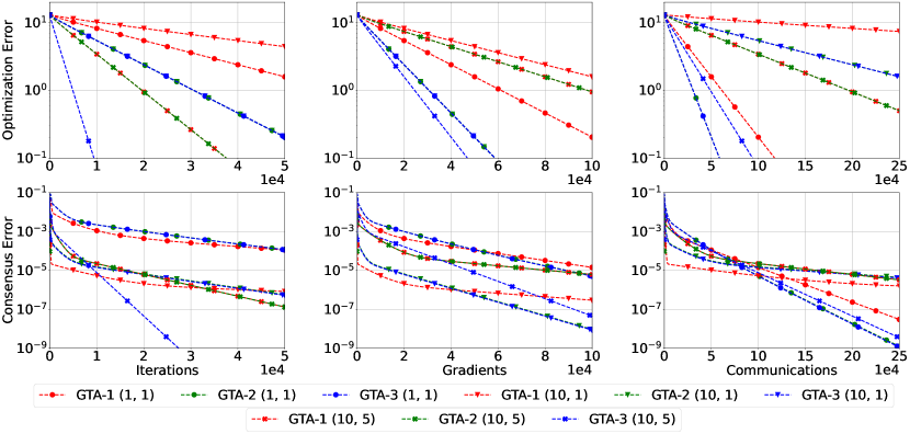
Figure 1: Optimization Error ($\|\mkern 1.5mu\overline{\mkern-1.5mux}_{k}-x^{*}\|_{2}$) and Consensus Error ($\|\mathbf{x}_{k}-\bar{\mathbf{x}}_{k}\|_{2}$) of GTA-1, GTA-2 and GTA-3 with respect to number of iterations, communications and gradient evaluations for a synthetic quadratic problem ($n=16$, $d=10$, $\kappa=10^{4}$) over a cyclic network ($\beta=0.992$).

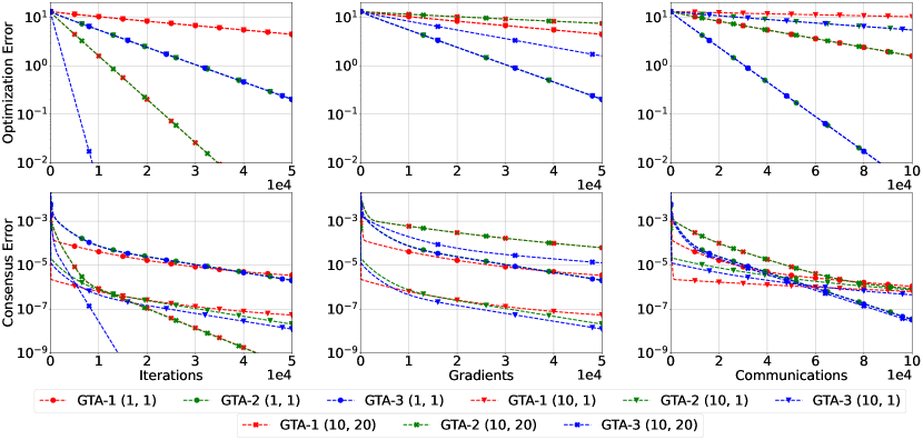
Figure 2: Optimization Error ($\|\mkern 1.5mu\overline{\mkern-1.5mux}_{k}-x^{*}\|_{2}$) and Consensus Error ($\|\mathbf{x}_{k}-\bar{\mathbf{x}}_{k}\|_{2}$) of GTA-1, GTA-2 and GTA-3 with respect to number of iterations, communications and gradient evaluations for a synthetic quadratic problem ($n=16$, $d=10$, $\kappa=10^{4}$) over star network($\beta=0.95$).

4.2 Binary Classification Logistic Regression

Next, we consider $\ell_{2}$-regularized binary classification logistic regression problems of the form

$$f(x) =\frac{1}{n}\sum_{i=1}^{n}\frac{1}{n_{i}}\log(1+e^{-b_{i}^{T}A_{i}x})+\frac{1}{n_{i}}\|x\|_{2}^{2},$$

where each node $i\in\{1,2,..,n\}$ has a portion of data samples $A_{i}\in\mathbb{R}^{n_{i}\times d}$ and corresponding labels $b_{i}\in\{0,1\}^{n_{i}}$. Experiments were performed over the mushroom dataset ($n=16$, $d=117$, $\sum_{i=1}^{n}n_{i}=8124$) and the australian dataset ($n=16$, $d=41$, $\sum_{i=1}^{n}n_{i}=690$) [12].

Figs. 3 and 4 show the performance of GTA-1, GTA-2 and GTA-3 over a cyclic network ($\beta=0.992$) for the mushroom dataset and a star network for the australian dataset ($\beta=0.95$), respectively. Similar observations to those made for the quadratic problem with respect to the effect of performing multiple communication and computation steps can also be made for these problems. Additionally, we observe that GTA-3 outperforms GTA-2 on these problems. We should note that although GTA-3 performs the best within these experiments, it also brings certain implementation constraints; see Section 2.

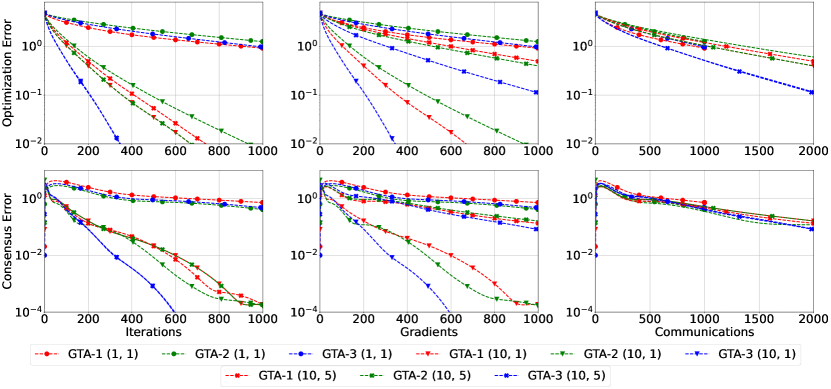
Figure 3: Optimization Error ($\|\mkern 1.5mu\overline{\mkern-1.5mux}_{k}-x^{*}\|_{2}$) and Consensus Error ($\|\mathbf{x}_{k}-\bar{\mathbf{x}}_{k}\|_{2}$) of GTA-1, GTA-2 and GTA-3 with respect to number of iterations, communications and gradient evaluations for binary logistic regression on Mushroom dataset ($n=16$, $d=117$, $\sum_{i=1}^{n}n_{i}=8124$) over cyclic network ($\beta=0.992$).

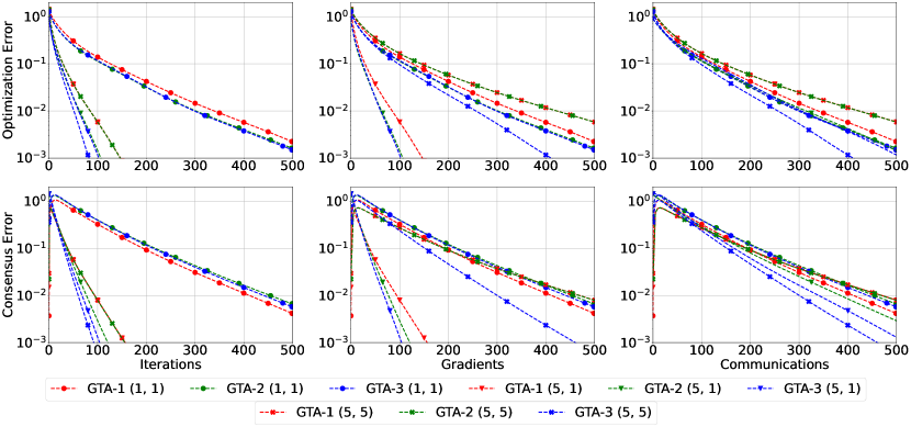
Figure 4: Optimization Error ($\|\mkern 1.5mu\overline{\mkern-1.5mux}_{k}-x^{*}\|_{2}$) and Consensus Error ($\|\mathbf{x}_{k}-\bar{\mathbf{x}}_{k}\|_{2}$) of GTA-1, GTA-2 and GTA-3 with respect to number of iterations, communications and gradient evaluations for binary logistic regression on Australian dataset ($n=16$, $d=41$, $\sum_{i=1}^{n}n_{i}=690$) over star network ($\beta=0.95$).

5 Final Remarks

In this paper, we have proposed a framework that unifies and generalizes communication strategies in gradient tracking methods with flexibility in the number of communication and computation steps performed at every iteration. We have established convergence guarantees for the proposed gradient tracking framework. Specifically, we have shown linear convergence for the general framework and the special cases of gradient tracking methods. Moreover, we have shown the positive influence of performing multiple communication steps at every iteration on the convergence rate and provide results that allow for the direct comparison of popular gradient tracking methods. Our experiments on quadratic and logistic regression problems illustrate the effects of different communication strategies and the benefits of the flexibility in terms of iterations and number of communication and computation steps. The advantages of the proposed framework can be further realized when the actual cost, i.e., a combination of the complexity of both communication and computation steps that is application specific, is considered. Finally, the algorithmic framework can be extended to other interesting settings such as nonconvex problems, stochastic local information, asynchronous updates, and higher-order approaches.

References

- [1] Sulaiman A Alghunaim, Ernest K Ryu, Kun Yuan, and Ali H Sayed. Decentralized proximal gradient algorithms with linear convergence rates. IEEE Transactions on Automatic Control, 66(6):2787–2794, 2020.
- [2] Yossi Arjevani, Joan Bruna, Bugra Can, Mert Gurbuzbalaban, Stefanie Jegelka, and Hongzhou Lin. Ideal: Inexact decentralized accelerated augmented lagrangian method. Advances in Neural Information Processing Systems, 33:20648–20659, 2020.
- [3] Brian Baingana, Gonzalo Mateos, and Georgios B Giannakis. Proximal-gradient algorithms for tracking cascades over social networks. IEEE Journal of Selected Topics in Signal Processing, 8(4):563–575, 2014.
- [4] Albert S Berahas, Raghu Bollapragada, Nitish Shirish Keskar, and Ermin Wei. Balancing communication and computation in distributed optimization. IEEE Transactions on Automatic Control, 64(8):3141–3155, 2018.
- [5] Albert S. Berahas, Raghu Bollapragada, and Ermin Wei. On the convergence of nested decentralized gradient methods with multiple consensus and gradient steps. IEEE Transactions on Signal Processing, 69:4192–4203, 2021.
- [6] Albert S Berahas, Charikleia Iakovidou, and Ermin Wei. Nested distributed gradient methods with adaptive quantized communication. In 2019 IEEE 58th Conference on Decision and Control (CDC), pages 1519–1525. IEEE, 2019.
- [7] Dimitri Bertsekas and John Tsitsiklis. Parallel and distributed computation: numerical methods. Athena Scientific, 2015.
- [8] Yongcan Cao, Wenwu Yu, Wei Ren, and Guanrong Chen. An overview of recent progress in the study of distributed multi-agent coordination. IEEE Transactions on Industrial informatics, 9(1):427–438, 2012.
- [9] Annie I Chen and Asuman Ozdaglar. A fast distributed proximal-gradient method. In 2012 50th Annual Allerton Conference on Communication, Control, and Computing (Allerton), pages 601–608. IEEE, 2012.
- [10] Patrick L Combettes and Jean-Christophe Pesquet. Proximal splitting methods in signal processing. In Fixed-point algorithms for inverse problems in science and engineering, pages 185–212. Springer, 2011.
- [11] Paolo Di Lorenzo and Gesualdo Scutari. Next: In-network nonconvex optimization. IEEE Transactions on Signal and Information Processing over Networks, 2(2):120–136, 2016.
- [12] Dheeru Dua and Casey Graff. UCI machine learning repository, 2017.
- [13] Pedro A Forero, Alfonso Cano, and Georgios B Giannakis. Consensus-based distributed support vector machines. Journal of Machine Learning Research, 11(5), 2010.
- [14] Eduard Gorbunov, Filip Hanzely, and Peter Richtárik. Local sgd: Unified theory and new efficient methods. In International Conference on Artificial Intelligence and Statistics, pages 3556–3564. PMLR, 2021.
- [15] Roger A Horn and Charles R Johnson. Matrix analysis. Cambridge university press, 2012.
- [16] Dušan Jakovetić, José MF Moura, and Joao Xavier. Linear convergence rate of a class of distributed augmented lagrangian algorithms. IEEE Transactions on Automatic Control, 60(4):922–936, 2014.
- [17] Sai Praneeth Karimireddy, Satyen Kale, Mehryar Mohri, Sashank Reddi, Sebastian Stich, and Ananda Theertha Suresh. Scaffold: Stochastic controlled averaging for federated learning. In International Conference on Machine Learning, pages 5132–5143. PMLR, 2020.
- [18] Xiang Li, Kaixuan Huang, Wenhao Yang, Shusen Wang, and Zhihua Zhang. On the convergence of fedavg on non-iid data. arXiv preprint arXiv:1907.02189, 2019.
- [19] Qing Ling, Wei Shi, Gang Wu, and Alejandro Ribeiro. Dlm: Decentralized linearized alternating direction method of multipliers. IEEE Transactions on Signal Processing, 63(15):4051–4064, 2015.
- [20] Sindri Magnússon. Bandwidth Limited Distributed Optimization with Applications to Networked Cyberphysical Systems. PhD thesis, KTH Royal Institute of Technology, 2017.
- [21] Gabriel Mancino-Ball, Yangyang Xu, and Jie Chen. A decentralized primal-dual framework for non-convex smooth consensus optimization. arXiv preprint arXiv:2107.11321, 2021.
- [22] Fatemeh Mansoori and Ermin Wei. Flexpd: A flexible framework of first-order primal-dual algorithms for distributed optimization. IEEE Transactions on Signal Processing, 69:3500–3512, 2021.
- [23] Konstantin Mishchenko, Grigory Malinovsky, Sebastian Stich, and Peter Richtárik. Proxskip: Yes! local gradient steps provably lead to communication acceleration! finally! arXiv preprint arXiv:2202.09357, 2022.
- [24] Aritra Mitra, Rayana Jaafar, George J Pappas, and Hamed Hassani. Linear convergence in federated learning: Tackling client heterogeneity and sparse gradients. Advances in Neural Information Processing Systems, 34:14606–14619, 2021.
- [25] Aryan Mokhtari, Qing Ling, and Alejandro Ribeiro. Network newton distributed optimization methods. IEEE Transactions on Signal Processing, 65(1):146–161, 2016.
- [26] Angelia Nedic, Alex Olshevsky, and Wei Shi. Achieving geometric convergence for distributed optimization over time-varying graphs. SIAM Journal on Optimization, 27(4):2597–2633, 2017.
- [27] Angelia Nedić, Alex Olshevsky, Wei Shi, and César A Uribe. Geometrically convergent distributed optimization with uncoordinated step-sizes. In 2017 American Control Conference (ACC), pages 3950–3955. IEEE, 2017.
- [28] Angelia Nedic and Asuman Ozdaglar. Distributed subgradient methods for multi-agent optimization. IEEE Transactions on Automatic Control, 54(1):48–61, 2009.
- [29] Yurii Nesterov. Introductory lectures on convex programming volume i: Basic course. Lecture notes, 3(4):5, 1998.
- [30] Edward Duc Hien Nguyen, Sulaiman A Alghunaim, Kun Yuan, and César A Uribe. On the performance of gradient tracking with local updates. arXiv preprint arXiv:2210.04757, 2022.
- [31] Joel B Predd, Sanjeev R Kulkarni, and H Vincent Poor. Distributed learning in wireless sensor networks. John Wiley & Sons: Chichester, UK, 2007.
- [32] Shi Pu and Angelia Nedić. Distributed stochastic gradient tracking methods. Mathematical Programming, 187(1):409–457, 2021.
- [33] Shi Pu, Wei Shi, Jinming Xu, and Angelia Nedić. Push–pull gradient methods for distributed optimization in networks. IEEE Transactions on Automatic Control, 66(1):1–16, 2020.
- [34] Guannan Qu and Na Li. Harnessing smoothness to accelerate distributed optimization. IEEE Transactions on Control of Network Systems, 5(3):1245–1260, 2017.
- [35] Ali H Sayed. Diffusion adaptation over networks. In Academic Press Library in Signal Processing, volume 3, pages 323–453. Elsevier, 2014.
- [36] Wei Shi, Qing Ling, Gang Wu, and Wotao Yin. Extra: An exact first-order algorithm for decentralized consensus optimization. SIAM Journal on Optimization, 25(2):944–966, 2015.
- [37] Wei Shi, Qing Ling, Kun Yuan, Gang Wu, and Wotao Yin. On the linear convergence of the admm in decentralized consensus optimization. IEEE Transactions on Signal Processing, 62(7):1750–1761, 2014.
- [38] Ying Sun, Gesualdo Scutari, and Amir Daneshmand. Distributed optimization based on gradient tracking revisited: Enhancing convergence rate via surrogation. SIAM Journal on Optimization, 32(2):354–385, 2022.
- [39] Akhil Sundararajan, Bin Hu, and Laurent Lessard. Robust convergence analysis of distributed optimization algorithms. In 2017 55th Annual Allerton Conference on Communication, Control, and Computing (Allerton), pages 1206–1212. IEEE, 2017.
- [40] Konstantinos I Tsianos, Sean Lawlor, and Michael G Rabbat. Consensus-based distributed optimization: Practical issues and applications in large-scale machine learning. In 2012 50th annual allerton conference on communication, control, and computing (allerton), pages 1543–1550. IEEE, 2012.
- [41] Ermin Wei and Asuman Ozdaglar. On the o (1= k) convergence of asynchronous distributed alternating direction method of multipliers. In 2013 IEEE Global Conference on Signal and Information Processing, pages 551–554. IEEE, 2013.
- [42] Jinming Xu, Ye Tian, Ying Sun, and Gesualdo Scutari. Distributed algorithms for composite optimization: Unified framework and convergence analysis. IEEE Transactions on Signal Processing, 69:3555–3570, 2021.
- [43] Jinming Xu, Shanying Zhu, Yeng Chai Soh, and Lihua Xie. Augmented distributed gradient methods for multi-agent optimization under uncoordinated constant stepsizes. In 2015 54th IEEE Conference on Decision and Control (CDC), pages 2055–2060. IEEE, 2015.
- [44] Shengjun Zhang, Xinlei Yi, Jemin George, and Tao Yang. Computational convergence analysis of distributed optimization algorithms for directed graphs. In 2019 IEEE 15th International Conference on Control and Automation (ICCA), pages 1096–1101. IEEE, 2019.
- [45] Yuchen Zhang and Lin Xiao. Communication-efficient distributed optimization of self-concordant empirical loss. Large-Scale and Distributed Optimization, pages 289–341, 2018.
- [46] Ke Zhou and Stergios I Roumeliotis. Multirobot active target tracking with combinations of relative observations. IEEE Transactions on Robotics, 27(4):678–695, 2011.