Sequential Knockoffs for Variable Selection in Reinforcement Learning

Abstract

In real-world applications of reinforcement learning, it is often challenging to obtain a state representation that is parsimonious and satisfies the Markov property without prior knowledge. Consequently, it is common practice to construct a state which is larger than necessary, e.g., by concatenating measurements over contiguous time points. However, needlessly increasing the dimension of the state can slow learning and obfuscate the learned policy. We introduce the notion of a minimal sufficient state in a Markov decision process (MDP) as the smallest subvector of the original state under which the process remains an MDP and shares the same optimal policy as the original process. We propose a novel sequential knockoffs (SEEK) algorithm that estimates the minimal sufficient state in a system with high-dimensional complex nonlinear dynamics. In large samples, the proposed method controls the false discovery rate, and selects all sufficient variables with probability approaching one. As the method is agnostic to the reinforcement learning algorithm being applied, it benefits downstream tasks such as policy optimization. Empirical experiments verify theoretical results and show the proposed approach outperforms several competing methods in terms of variable selection accuracy and regret.

Keywords: Reinforcement learning, Variable selection, Sequential knockoffs, False discovery rate control, Power analysis

1 Introduction

Interest in reinforcement learning (RL, Sutton & Barto, 2018) has increased dramatically in recent years due in part to a number of high-profile successes in games (Mnih et al., 2013, 2015), autonomous driving (Sallab et al., 2017), and precision medicine (Tsiatis et al., 2019). However, despite theoretical and computational advances, real-world application of RL remains difficult. A primary challenge is dealing with high-dimensional state representations. Such representations occur naturally in systems with high-dimensional measurements, like images or audio, but can also occur when the system state is constructed by concatenating a series of measurements over a contiguous block of time. A high-dimensional state—when a more parsimonious one would suffice—dilutes the efficiency of learning algorithms and makes the estimated optimal policy harder to interpret. Thus, methods for removing uninformative or redundant variables from the state are of tremendous practical value.

We develop a general variable selection algorithm for offline RL, which aims to learn an optimal policy using only logged data, i.e., without any additional online interaction. Our contributions can be summarized as follows: (i) we formally define a minimal sufficient state for an MDP and argue that it is an appropriate target by which to design and evaluate variable selection methods in RL; (ii) we show that naïve variable selection methods based on the state or reward alone need not recover the minimal sufficient state; (iii) we propose a novel sequential knockoffs (SEEK) algorithm that applies with general black-box learning methods, and, under a $\beta$-mixing condition, consistently recovers the minimal sufficient state, and controls the false discovery rate (FDR, the ratio of the number of selected irrelevant variables to the number of selected variables); and (iv) we develop a novel algorithm to estimate the $\beta$-mixing coefficients of an MDP. The algorithm in (iv) is important in its own right as it applies to a number of applications beyond RL (McDonald et al., 2015).

1.1 Related Work

Our work uses the idea of knockoff variables, also known as pseudo-variables, for variable selection. Intuitively, knockoff methods augment the observed data with noise variables (knockoffs) and use the rate at which these noise variables are selected by a variable selection algorithm to characterize the algorithm’s operating characteristics (Wu et al., 2007; Barber & Candès, 2015). A key strength of knockoff methods is their generality. Knockoffs can be used to estimate (and subsequently tune) the FDR of general black-box variable selection algorithms (Candès et al., 2018; Lu et al., 2018; Romano et al., 2020; Zhu et al., 2021). Being algorithm agnostic is especially appealing in a vibrant field like RL, where algorithms are emerging and evolving rapidly. Unfortunately, it is not possible to directly export existing knockoff methods to RL because knockoffs have been developed almost exclusively in the regression setting under the assumption of independent observations; an assumption which is clearly violated in RL settings. One exception is a recent proposal for knockoffs in time series data (Chi et al., 2021). However, as will show in Section 3, applying this one-step approach to the states in an MDP need not recover the minimal sufficient state.

In the statistics literature, RL is closely related to a growing line of works on learning optimal dynamic treatment regimes in precision medicine (see e.g., Kosorok & Laber, 2019, for an overview). A number of variable selection approaches have been proposed to estimate a parsimonious treatment regime (Gunter et al., 2011; Qian & Murphy, 2011; Song et al., 2015; Fan et al., 2016; Shi et al., 2018; Zhang & Zhang, 2018; Qi et al., 2020; Bian et al., 2021). However, these methods are designed for a short time horizon (e.g., 2-5 times points), and are not applicable to long or infinite horizons which are common in RL.

Relative to its practical importance, variable selection for RL is under-explored. In the computer science literature, Kroon & Whiteson (2009) and Guo & Brunskill (2017) studied variable selection in factored Markov decision processes (MDPs). Nguyen et al. (2013) applied penalized logistic regression to learn transition functions in structured MDPs. In MDPs without any specific structure, a common approach is penalized estimation. This includes temporal-difference (TD) learning with LASSO (Tibshirani, 1996) or the Dantzig selector (Candes & Tao, 2007); see e.g., Kolter & Ng (2009); Ghavamzadeh et al. (2011); Geist et al. (2012). In a similar spirit, Hao et al. (2021) recently proposed combining LASSO with fitted Q-iteration (Ernst et al., 2005, FQI). However, these methods are designed for linear function approximation whereas our goal is to develop variable selection methods that are not reliant on a specific algorithm or functional form.

Our proposal is also related to a line of research on abstract representation learning in the RL literature, where the goal is to construct a state abstraction, defined as a mapping from the original state space to a much smaller abstraction space that preserves many properties of the original MDP (see e.g. Jiang, 2018, for an overview). In particular, bisimulation corresponds to a class of abstraction methods where the system preserves the Markov property and the optimal policy based on the resulting abstract MDP can achieve the same value as that of the original MDP (Dean & Givan, 1997; Li et al., 2006). However, identifying the “minimal” bisimulation is NP-hard (Givan et al., 2003). Existing solutions either focus on building an approximate bisimulation (Ferns et al., 2011; Ferns & Precup, 2014; Zhang et al., 2020), or learning a Markov state abstraction while ignoring the reward signal (Allen et al., 2021). These methods share similar ideas with existing dimension reduction and representation learning methods developed in the RL literature (see e.g., Wang et al., 2017; Uehara et al., 2021).

In contrast with the aforementioned state abstraction and dimension reduction methods, we focus on selecting a subvector of the original state rather than engineering new features. This approach is advantageous in settings such as mobile-health where an interpretable and parsimonious learned policy is important for generating new clinical insights. However, our methods can also be used with basis expansions constructed from the original state such as splines or tile codings. Another advantage of our approach is its computational efficiency, we show that SEEK is guaranteed to terminate after no more than $p$ iterations where $p$ is the dimension of the state.

1.2 Organization of the paper

In Section 2, we review the Model-X knockoffs method for variable selection in regression, and describe the challenges brought by sequential decision-making. In Section 3, we formulate the variable selection problem in RL and introduce the proposed minimal sufficient state. In Section 4, we present the sequential knockoffs (SEEK) procedure for identifying the minimal sufficient state. In Section 5, we show our method controls both modified FDR and FDR, with power approaching one asymptotically. Finally, we investigate the empirical performance of our method via extensive simulations and a real data analysis in Sections 6 and 7. Some implementation details, technical proofs, and additional theoretical and numerical results are available in the Supplementary Material.

2 Preliminaries: Variable Selection with Knockoffs and Challenges of Adapting to RL

We briefly review the Model-X knockoffs algorithm in the regression setting (Candès et al., 2018). Suppose that the observed data are $\mathcal{D}=\left\{(\mathbf{X}_{i},\mathbf{Y}_{i})\right\}_{i=1}^{n}$ which comprise $n$ i.i.d. copies of $(\mathbf{X},\mathbf{Y})$, where $\mathbf{X}=\left(X_{1},\ldots,X_{p}\right)^{\top}\in\mathbb{R}^{p}$ is a vector of inputs and $\mathbf{Y}\in\mathbb{R}^{d}$ is a (possibly multivariate) response. We say $X_{j}$ is a null variable if it is conditionally independent of $\mathbf{Y}$ given the other variables; a variable that is not null is said to be significant. Let $\mathcal{H}_{0}\subseteq\left\{1,\ldots,p\right\}$ be the indices of the null variables and $\mathcal{I}=\mathcal{H}_{0}^{c}$ the indices of important variables. Given an estimator $\widehat{\mathcal{I}}$ of $\mathcal{I}$ constructed from $\mathcal{D}$ and some pre-specified level $q\in(0,1)$, the false discovery rate (FDR) and modified FDR (mFDR) associated with $\widehat{\mathcal{I}}$ are given by $\mathbb{E}\{\#(\widehat{\mathcal{I}}\bigcap\mathcal{H}_{0})/\max(1,\#\widehat{\mathcal{I}})\}$ and $\mathbb{E}\{\#(\widehat{\mathcal{I}}\bigcap\mathcal{H}_{0})/(1/q+\#\widehat{\mathcal{I}})\}$, respectively. The goal of knockoffs is to construct an estimator of $\mathcal{I}$ which ensures the (m)FDR is below $q$.

The key innovation of noise-variable addition methods is the construction of knockoff variables $\widetilde{\mathbf{X}}=\left(\widetilde{X}_{1},\ldots,\widetilde{X}_{p}\right)^{\top}\in\mathbb{R}^{p}$ which mimic the covariates $\mathbf{X}$ except that they are conditionally independent of the response and thus known to be null variables. Knockoffs are constructed so that they satisfy: (1) $\widetilde{\mathbf{X}}\perp\!\!\!\perp\mathbf{Y}|\mathbf{X}$ (i.e., conditional independence of the response); (2) $(\mathbf{X},\widetilde{\mathbf{X}})_{\text{swap}(B)}\overset{d}{=}(\mathbf{X},\widetilde{\mathbf{X}})$ for any subset $B\subset\{1,2,\ldots,p\}$ (i.e., exchangeability in distribution), where $(\mathbf{X},\widetilde{\mathbf{X}})_{\text{swap}(B)}$ is the vector formed by switching the $j$-th entries of $\mathbf{X}$ and $\widetilde{\mathbf{X}}$ for each $j\in B$. Once $\widetilde{\mathbf{X}}$ is obtained, let $\widetilde{\mathcal{D}}=\{(\mathbf{X}_{i},\widetilde{\mathbf{X}}_{i},\mathbf{Y}_{i})\}_{i=1}^{n}$ denote an augmented version of the observed data in which each $\mathbf{X}_{i}$ is augmented with a knockoff variable $\widetilde{\mathbf{X}}_{i}$.

From $\widetilde{\mathcal{D}}$ we compute feature importance statistics $Z_{j}$ and $\widetilde{Z}_{j}$ for each variable $X_{j}$ and its knockoff $\widetilde{X}_{j}$ (see Section 5.2 for specific examples). Let $f:\mathbb{R}^{2}\rightarrow\mathbb{R}$ be an anti-symmetric function, i.e., $f(u,v)=-f(v,u)$ for all $u,v\in\mathbb{R}^{2}$, and define $W_{j}=f(Z_{j},\widetilde{Z}_{j})$ so that higher values of $W_{j}$ are associated with stronger evidence that $X_{j}$ is significant. Given a target FDR level $q$, the $j$th variable is selected if $W_{j}$ is no less than some threshold $\tau_{q}$ (or $\tau_{q+}$ in knockoffs+ method). For instance, the set of selected variables is $\widehat{\mathcal{I}}=\{j\,:\,W_{j}\geq\tau_{q}\}$ with

$$\tau_{q}=\min\left\{\tau>0\,:\,\#\{j\,:\,W_{j}\leq-\tau\}/\#\{j\,:\,W_{j}\geq\tau\}\leq q\right\},$$

in the knockoffs method. See the related part in Supplementary Material B for more details. As long as the $W_{j}$’s satisfy the flip-sign property (see Section 5.2), the knockoffs procedure controls the FDR (and mFDR).

Model-X knockoffs possess a number of desirable statistical properties. First, it provides non-asymptotic control of the FDR given the covariate distribution. Second, it does not depend on any specific model structure between the outcome and covariates; thus, the knockoffs method applies in nonlinear and high-dimensional settings. Finally, the true positive rate is near optimal in a wide class of problems (Fan et al., 2019; Weinstein et al., 2020; Wang & Janson, 2020; Ke et al., 2020). However, the derivation of these theoretical properties relies critically on the assumption that the observed data are independent—an assumption that is clearly violated in RL problems. Another challenge is that the definition of a significant variable in an MDP is less obvious than it is in regression. Attempting to mimic the regression setting, say by defining significant state variables as those associated with the reward will fail to capture variables which impact cumulative reward indirectly through state transitions. Conversely, if one defines the ‘outcome’ as the reward concatenated with the next state, then the knockoffs procedure will incorrectly select those which are associated with the next state but have no effect on the (present or future) reward. We propose to define variable significance in RL in terms of the minimal sufficient state which we introduce in the next section.

3 Minimal Sufficient State and Model-based Selections

We model the observed data as a time-homogeneous MDP, denoted by $\mathcal{M}=(\mathcal{S},\mathcal{A},r,\mathcal{P},\gamma)$, with a state space $\mathcal{S}=\prod_{j=1}^{p}\mathcal{S}_{j}\subseteq\mathbb{R}^{p}$, a discrete action space $\mathcal{A}$, a mean reward function $r:\mathcal{S}\times\mathcal{A}\rightarrow\mathbb{R}$, a transition kernel $\mathcal{P}:\mathcal{S}\times\mathcal{S}\times\mathcal{A}\rightarrow\mathbb{R}^{+}$, and a discount factor $\gamma\in[0,1)$ (see Puterman, 2014, for additional background on MDPs). Let $(\mathbf{S}_{t},A_{t},R_{t})$ denote the state-action-reward triplet at time $t$. The dynamic system is Markovian such that both the reward and next state, $R_{t}$ and $\mathbf{S}_{t+1}$, are conditionally independent of the past data history given the current state and action, $\mathbf{S}_{t}$ and $A_{t}$. The transition kernel defines the conditional distribution of the next state given the current state-action pair. The reward function, $r$, characterizes the conditional mean of $R_{t}$ given $\mathbf{S}_{t}$ and $A_{t}$. We further assume the reward is bounded, i.e., there exists constant $R_{\max}$ such that $|R_{t}|\leq R_{\max}$ almost surely for any $t$. We use $(\mathbf{S}_{t},A_{t},R_{t},\mathbf{S}_{t+1})$ to refer to a generic state-action-reward-next state tuple. For any $\mathbf{\nu}\in\mathbb{R}^{p}$ and index set $G\subseteq\{1,2,\ldots,p\}$, let $\mathbf{\nu}_{G}=\{\nu_{g}\,\mid\,g\in G\}$; thus, $\mathbf{S}_{t,G}$ is the subvector of state $\mathbf{S}_{t}$ indexed by components in $G$. Let $G^{c}=\{1,\ldots,p\}\setminus G$ be the complement of $G$.

Definition 1 (Sufficient State).

We say $\mathbf{S}_{G}$ is a sufficient state in an MDP if $R_{t}\perp\!\!\!\perp\mathbf{S}_{t,G^{c}}\,|\,(\mathbf{S}_{t,G},A_{t})$ and $\mathbf{S}_{t+1,G}\perp\!\!\!\perp\mathbf{S}_{t,G^{c}}\,|\,(\mathbf{S}_{t,G},A_{t})$, for all $t\geq 0$.

This definition of sufficiency is weaker than the condition that $R_{t}$ and $\mathbf{S}_{t+1,G}$ are jointly conditionally independent of $\mathbf{S}_{t,G^{c}}$. Furthermore, a sufficient state always exists as $\mathbf{S}_{t}$ itself is sufficient. The following results justify the use of the term sufficient in Definition 1.

Proposition 1.

If $\mathbf{S}_{G}$ is a sufficient state, then there exists an optimal policy that depends only on $\mathbf{S}_{G}$.

Proposition 2.

If $\mathbf{S}_{G}$ is a sufficient state, then the process $\{\left(\mathbf{S}_{t,G},A_{t},R_{t}\right)\}_{t\geq 0}$ forms a time-homogeneous MDP.

Proposition 1 allows us to focus on policies that are functions of sufficient states only. Most existing RL algorithms require the data-generating process to follow an MDP model, Proposition 2 implies that once the sufficient state is identified, these algorithms can be directly applied to the reduced process $\{\left(\mathbf{S}_{t,G},A_{t},R_{t}\right)\}_{t\geq 0}$. A low-dimensional sufficient state can enhance the performance of policy optimization and reduce computational costs. Therefore we aim to identify minimal sufficient state, which is defined as follows.

Definition 2 (Minimal Sufficient State).

We say $\mathbf{S}_{G}$ is a minimal sufficient state if it is the sufficient state with the minimal dimension among all sufficient states.

Below we show that the minimal sufficient state is well-defined and unique under mild conditions.

Proposition 3.

The minimal sufficient state always exists. Furthermore, if the transition kernel is strictly positive, then the minimal sufficient state is unique.

Our goal is to identify the minimal sufficient state using batch data. To provide insights into this problem and to motivate our proposed approach, we first discuss two extensions of variable selection methods for supervised learning to MDPs which fail to recover the minimal sufficient state.

Reward-only approach: One approach to extending variable selection methods for regression to the MDP setting is to treat the state and action as covariates and the reward as the outcome, and then apply an existing regression method as if the data were comprised of i.i.d. input (state, action) output (reward) pairs. This approach will fail to identify components of the state which do not affect immediate reward but rather affect long-term rewards through their impact on the next state. Thus, this approach can have a high false negative rate, need not be consistent for a sufficient state, and a process indexed by a state constructed using this approach does not need to satisfy the Markov property.

One-step approach: To capture components of the state associated with both short- and long-term impacts on the reward, one can treat the reward and the next state jointly as a multivariate outcome and the current state-action pair as the input. With this setup, one can apply variable selection techniques for multiple-outcome regression. This approach was considered by Tangkaratt et al. (2016) in the context of dimension reduction. While this approach can consistently remove pure noise variables, it will fail to remove time-dependent variables that do not affect cumulative reward. Consequently, as shown below, it will identify a sufficient state but need not identify a minimally sufficient one.

Proposed iterative approach: The one-step approach fails to identify the minimal sufficient state because the response includes the entire next state vector (including those which are unrelated to the cumulative reward). Conceptually, one could avoid this by taking every possible subset $G$ of $\left\{1,\ldots,p\right\}$, and testing the sufficiency condition in Definition 1. However, such an approach is not scalable as it requires examining $2^{p}$ subsets and, for each, conducting multivariate conditional independence tests. As a result, we propose a sequential knockoffs procedure that is (asymptotically) equivalent to such a procedure while requiring at most $p$ iterations to converge. At a high level, the algorithm proceeds as follows. At the first iteration, a variable selection algorithm is applied to identify, $\widehat{G}_{1}$, the components of state significant for predicting the immediate reward. The second iteration uses the selection algorithm to identify, $\widehat{G}_{2}$, the components of state significant for predicting $\mathbf{S}_{t+1,\widehat{G}_{1}}$. Then recursively for $j\geq 2$, we identify the set of variables $\widehat{G}_{j}$ which predict $\mathbf{S}_{t+1,\widehat{G}_{j-1}}$. The algorithm terminates when $\widehat{G}_{j}=\widehat{G}_{j+1}$. As the sets $\widehat{G}_{j}$ are monotonically non-decreasing, the algorithm terminates in no more than $p$ steps.

A numerical example: We conduct a simulation example to illustrate the advantage of the iterative selection method. In this example, the dimension of the state is $20$ and the index set of the minimal sufficient state is $G_{\text{M}}=\{1,2\}$. The generative model is such that $S_{t,1}$ directly influences $R_{t}$ whereas $S_{t,2}$ affects $S_{t+1,1}$ and hence has an indirect effect on the reward. The remaining state variables can be divided into two groups. The first group, $G_{\text{AR}}=\{3,\ldots,11\}$ indexes state variables whose transitions are independent and follow a first-order autoregressive (AR(1)) model, i.e.,

$$\mathbb{P}(S_{t+1,j}|\mathbf{S}_{t},A_{t})=\mathbb{P}(S_{t+1,j}|S_{t,j}),\qquad j=3,\ldots,11.$$

The second group $G_{\text{WN}}=\{12,\ldots,20\}$ indexes state variables which are i.i.d. white noise across all decision points. We conduct a numerical study using the above three approaches, and summarize the results in Figure 1 and Table 1 under a fixed target FDR of 0.3, aggregated over 20 runs. The implementation details of these methods is presented in Section 4. It can be seen from Table 1 that the reward-only method fails to select $S_{t,2}$, as expected. Furthermore, the one-step method selects all variables in $G_{\text{AR}}$ because they are time-dependent and contribute to the state transition function. In contrast, the iterative procedure (based on our proposed algorithm) avoids selecting redundant variables in $G_{\text{AR}}\cup G_{\text{WN}}$ and is thus more appealing. It can be seen from Figure 1 that the proposed algorithm controls the FDR and has a much larger area under the receiver operating characteristic curve among the three methods.

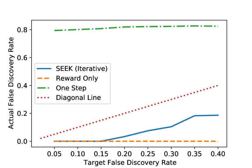
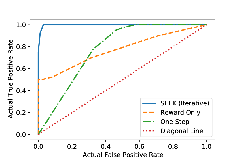
Figure 1: Receiver operating characteristic (ROC) curves for different methods in the toy example.

Table 1: Most frequently selected states by different methods in the toy example.

Method	Selected States
SEEK (Iterative)	[1, 2]
Reward-only Method	[1]
One-step Method	[1, 2, 3, 4, 5, 6, 7, 8, 9, 10, 11]

The following proposition summarizes the properties of these three approaches in the population level, i.e., assuming we have infinitely many observations.

Proposition 4.

Assume that one applies a selection-consistent algorithm for the above three approaches. Then, (i) there exists an MDP such that the state selected by the reward-only method is not sufficient; and (ii) the state selected by the one-step method is sufficient but not minimally sufficient. In addition, the iterative approach is able to correctly recover the minimal sufficient state for any MDP provided the transition kernel is strictly positive.

The preceding result does not depend on the selection algorithm being applied, only that it is selection consistent. Thus, this result is of independent interest as it provides a template for constructing variable selection methods for MDPs. In the remainder of this paper, we focus on developing the sequential knockoffs (SEEK) algorithm which extends Model-X knockoffs to the MDP setting combining the iterative procedure described above.

Remark 1.

Our proposed variable selection is general in that it benefits a wide variety of downstream analyses. For instance, one can evaluate any number of candidate policies, conduct exploratory analyses, etc. This is especially appealing with batch data collected in biomedical applications such as mobile-health (mHealth), in which there are numerous scientific questions of interest Tewari & Murphy (2017); Luckett et al. (2019); Liao et al. (2020). We note that if one were interested in, say, identifying variables present in the optimal policy, one could apply our method as an initial screening step and then apply an algorithm like penalized Q-learning to the reduced data.

4 SEEK: Sequential Knockoffs for Variable Selection

4.1 The Main Idea

In this section, we introduce our SEEK algorithm, which consists of three key steps. An outline is displayed in Algorithm 1. Additional implementation details can be found in Section B of the Supplementary Material. Suppose that we are given batch data $\mathcal{D}$ consisting of $N$ i.i.d. finite-horizon trajectories, each of length $T$, which can be summarized as $NT$ transition tuples. Note that observations within each trajectory are temporally dependent.

Step 1: Data splitting. We first split all $NT$ transition tuples in the batch data into $K$ non-overlapping sub-datasets, leading to a partition ${\cal D}=\{\mathcal{D}_{k},k\in[K]\}$ such that for each tuple, $\left(\mathbf{S}_{t},A_{t},R_{t},\mathbf{S}_{t+1}\right)\in\mathcal{D}_{k}$ if $t\,\textrm{mod}\,K={k-1}$. After the split, every two tuples within the same subset $\mathcal{D}_{k}$ either come from the same trajectory with a time gap of at least $K$, or belong to two different trajectories. When the system is $\beta$-mixing (Bradley, 2005), by an innovative use of Berbee’s coupling lemma (Berbee, 1987) and a careful choice of $K$, we can guarantee that all transition tuples within each subset $\mathcal{D}_{k}$ are “approximately independent.” See Supplementary Material Section C for a rigorous statement of this result. This justifies our iterative use of Model-X knockoffs on each $\mathcal{D}_{k}$ for finding the minimal sufficient state in the following steps. Finally, using majority vote, we aggregate the selection results from all the data subsets.

In Section 4.2, we develop a practical algorithm to adaptively select the number of splits $K$ under the $\beta$-mixing condition. When the system is non-ergodic, these $\mathcal{D}_{k}$’s can be constructed based on transition tuples from different trajectories to satisfy the independence assumption.

Step 2: Iterative selection. On each data subset $\mathcal{D}_{k}$, we implement our iterative selection approach using Model-X knockoffs. We first apply the aggregated knockoffs procedure (across actions, see Algorithm 2) to select the significant state variables for predicting the immediate reward only. Denote this initial selection by $\widehat{G}_{k,1}$. Subsequently, we treat all selected state variables in $\widehat{G}_{k,1}$ in the next decision point as a multivariate response and use aggregated knockoffs again to select state variables that are significant to this response. The final index set is denoted by $\widehat{G}_{k,2}$. We repeat this procedure to obtain $\widehat{G}_{k,3},\widehat{G}_{k,4},\ldots,$ where at each iteration we combine all previously selected state variables in the next-time-point to construct the multiple-response variable, until no more significant variables are found. The resulting index set of selected variables is denoted by $\widehat{G}_{k}$.

In our implementation, we adopt a second-order machine to construct knockoff variables. However, other construction approaches are possible, see approaches in Section B of the Supplementary Material. In addition, for linear systems, we set each feature importance statistics $Z_{j}$ (or $\widetilde{Z}_{j}$) to be the $\ell_{\infty}$-norm of the estimated regression coefficients in multivariate response regression. In nonlinear systems, we set $Z_{j}$ (or $\widetilde{Z}_{j}$) by the variable importance with general machine learning methods. See details in Section B.

Step 3: Majority vote. Compute the proportion of subsets in which variable $j$ was selected, $\widehat{p}_{j}=K^{-1}\sum_{k=1}^{K}\mathbb{I}\left(j\in\widehat{G}_{k}\right)$, and define the final selected set $\widehat{G}=\left\{j\,:\,\widehat{p}_{j}\geq\alpha\right\}$, where $\alpha\in(0,1)$ is a pre-specified threshold (e.g., 0.5).

The number of splits, $K$, is a potentially important tuning parameter. We discuss an adaptive (data-driven) procedure for selecting $K$ in the next section.

Algorithm 1 SEEK Algorithm

Input: Batch data $\mathcal{D}$, number of data subsets $K$, a target FDR level $q\in(0,0.5)$, and a threshold $\alpha\in(0,1)$ for the majority vote.

1:Split $\mathcal{D}$ evenly into $\{\mathcal{D}_{k},k\in[K]\}$ , with $NT/K$ transition tuples in each $\mathcal{D}_{k}$. Initialize all $\widehat{G}_{k}$’s as empty sets.

2:for $k=1,2,\ldots,K$ do

3:      Apply Algorithm 2 to all $(\mathbf{S},A,R)$ tuples in $\mathcal{D}_{k}$ with the target FDR level $q$. Denote the selected index set by $\widehat{G}_{k,1}$ and let $\widehat{G}_{k}=\widehat{G}_{k,1}$.

4:     for $j=2,3,...$ do

5:          Apply Algorithm 2 to all $(\mathbf{S},A,\mathbf{Y})$ tuples in $\mathcal{D}_{k}$ with $\mathbf{Y}=\mathbf{S}_{\widehat{G}_{k}}^{\prime}$ and the target FDR level $q$. Denote the selected index set by $\widehat{G}_{k,j}$.

6:         Break if $\widehat{G}_{k,j}\subset\widehat{G}_{k}$.

7:         Let $\widehat{G}_{k}=\widehat{G}_{k}\cup\widehat{G}_{k,j}$.

8:     end for

9:end for

10:Output: $\widehat{G}:=\{j\in\{1,\ldots,p\}:\sum_{1\leq k\leq K}\mathbb{I}(j\in\widehat{G}_{k})\geq\alpha K\}.$

Algorithm 2 Aggregated Knockoffs

Input: Batch data $\mathcal{D}_{k}$ consisting of random tuples $\{(\mathbf{S}_{i},A_{i},\mathbf{Y}_{i}):1\leq i\leq NT/K\}$, and a target FDR level $q\in(0,0.5)$.

1: Split $\mathcal{D}_{k}$ into $\{\mathcal{D}_{k}^{(a)},a\in[m]\}$ where $\mathcal{D}_{k}^{(a)}=\{(\mathbf{S}_{i},\mathbf{Y}_{i}):A_{i}=a\}$.

2:For each $a$, construct knockoff variables $\{\widetilde{\mathbf{S}}_{i}:A_{i}=a\}$.

3:Apply any machine learning algorithms (e.g., LASSO or random forest) to $\widetilde{\mathcal{D}}_{k}^{(a)}=\{(\mathbf{S}_{i},\widetilde{\mathbf{S}}_{i},\mathbf{Y}_{i}):A_{i}=a\}$ to construct feature importance statistics $Z_{j}^{(a)}$ and $\widetilde{Z}_{j}^{(a)}$ for $S_{j}$ and its knockoff variable, respectively, for each $j\in[p]$.

4:For each $j\in B$, set $Z_{j}=\max_{a}Z_{j}^{(a)}$, $\widetilde{Z}_{j}=\max_{a}\widetilde{Z}_{j}^{(a)}$ and $W_{j}=f(Z_{j},\widetilde{Z}_{j})$.

5:To implement the (standard) knockoffs method, set the threshold $\tau$ to

$$\min\left\{t>0:\frac{\displaystyle\#\{i\in[p]:W_{i}\leq-t\}}{\displaystyle\#\{i\in[p]:W_{i}\geq t\}}\leq q\right\},$$

Output $\widehat{G}_{k}=\{i\in[p]:W_{i}\geq\tau\}$.

6:To implement the knockoffs+ method, set the threshold $\tau_{+}$ to

$$\min\left\{t>0:\frac{\displaystyle 1+\#\{i\in[p]:W_{i}\leq-t\}}{\displaystyle\#\{i\in[p]:W_{i}\geq t\}}\leq q\right\},$$

Output $\widehat{G}_{k}=\{i\in[p]:W_{i}\geq\tau_{+}\}$.

4.2 Determining the number of splits

The performance of the proposed algorithm relies on the number of sub-datasets $K$ in the data splitting step. In this section, we present a practical algorithm to adaptively select $K$. A closer look at the proof for Theorem 1 reveals that for a given $K$, the FDR is bounded above by $q+(NT/K)\beta(K),$ where $\beta(K)$ denotes the $\beta$-mixing coefficient, measuring the temporal dependence of the MDP at lag $K$. See Definition C.4 for details. Thus, the choice of $K$ represents the following trade-off. On the one hand, when the system is $\beta$-mixing, we have $\lim_{K\to\infty}\beta(K)=0$. In theory, $K$ should diverge to infinity to avoid inflation of type-I error. On the other hand, $K$ should not be too large in order to guarantee that each data subset $\mathcal{D}_{k}$ has sufficiently many observations. To balance this trade-off, we propose to set $K$ to $K^{*}=\operatorname{argmin}\{k\geq 1:k^{-1}(NT)\beta(k)\leq\delta\}$ and estimate it via

$$\widehat{K}=\operatorname{argmin}\left\{k\geq 1:\frac{NT}{k}\widehat{\beta}(k)\leq\delta\right\},$$ (1)

where $\widehat{\beta}(\bullet)$ denotes the estimated mixing coefficient and $\delta$ denotes a pre-specified upper bound for the inflation of the type-I error (e.g., 0.01 or 0.05).

It remains to estimate the $\beta$-mixing coefficient. Existing solutions in the time series literature are based on histograms (McDonald et al., 2015) and thus suffer from the curse of dimensionality and perform poorly in problems with moderate dimension. Furthermore, it is not trivial to extend these methods to produce an accurate estimator of $K^{*}$ without imposing additional structure on the problem. To see this, suppose that $\beta(k)$ decays exponentially fast with respect to the lag $k$. Then $\beta(K^{*})$ is typically of the order $\delta(NT)^{-1}$ up to some logarithmic factor. Nonetheless, without additional assumptions, its estimation error is at least of the order $(NT)^{-1/2}\gg\delta(NT)^{-1}$. To address both challenges, we develop a novel three-step algorithm detailed below.

Step 1. Construct initial estimators of $\beta(1)$, $\cdots$, $\beta(K_{0})$ for a specified integer value of $K_{0}$ using a generic density estimator. Assuming both the behavior policy $\pi_{b}$ and the MDP are stationary, it follows that

$$\begin{split}\beta(k)&=\frac{1}{2}\sum_{a,a^{\prime}}\int_{s,s^{\prime}}|f(s)\pi_{b}(a|s)f(s^{\prime})\pi_{b}(a^{\prime}|s^{\prime})-f_{k}(s,s^{\prime})\pi_{b}^{\prime}(a|s,s^{\prime})\pi_{b}(a^{\prime}|s^{\prime})|\\ &=\frac{1}{2}\sum_{a}\int_{s,s^{\prime}}|f(s)\pi_{b}(a|s)f(s^{\prime})-f_{k}(s,s^{\prime})\pi_{b}^{\prime}(a|s,s^{\prime})|,\end{split}$$ (2)

where $f$ denotes the marginal state density function, $f_{k}$ denotes the joint distribution function of $(\mathbf{S}_{t},\mathbf{S}_{t+k})$, and $\pi_{b}^{\prime}$ is the conditional probability of the action given both the current state and the state after lag $k$. Thus, we first estimate $f$, $\pi_{b}$, $\pi_{b}^{\prime}$, and $f_{k}$, and then plug in these estimators to estimate $\beta(k)$. In practice, we use a Gaussian mixture model to approximate $f$ based on tuples $(\mathbf{S}_{t})$, and similarly to approximate $f_{k}$ based on tuples $(\mathbf{S}_{t},\mathbf{S}_{t+k})$. The behavior policy $\pi_{b}$ and the conditional probability $\pi_{b}^{\prime}$ can be estimated via supervised learning (e.g., multinomial logistic regression) using tuples $(\mathbf{S}_{t},A_{t})$ and tuples $(\mathbf{S}_{t},A_{t},\mathbf{S}_{t+k})$. In addition, we apply importance sampling to numerically calculate the integral in (2); details are in Section B.4. Let $\widetilde{\beta}(1)$, $\cdots$, $\widetilde{\beta}(K_{0})$ denote resulting estimators.

Step 2. The second step is to impose parametric structure on the mixing coefficients to refine the initial estimators and to estimate $\beta(k)$ for $k\geq K_{0}$. We assume $\beta(k)=a_{0}\exp(-b_{0}k)$ for some $a_{0},b_{0}>0$. However, our proposal also applies to settings where $\beta(k)$ decays polynomially fast in $k$. To estimate these model parameters, we assume the first-step estimators satisfy

$$\widetilde{\beta}(k)=\eta_{0}+a_{0}\exp(-b_{0}k)+\epsilon_{k},$$ (3)

for some $\eta_{0}>0$ and mean-zero random errors $\{\epsilon_{k}\}_{k=1}^{K_{0}}$. Here, $\eta_{0}$ and $\epsilon_{k}$ measure the bias and variance of the initial estimator. We use least squares to construct estimators $\widehat{\eta}_{0}$, $\widehat{a}_{0}$, $\widehat{b}_{0}$ and subsequently the final estimator $\widehat{\beta}(k)=\widehat{a}_{0}\exp(\widehat{b}_{0}k)$. It is worth mentioning that we remove the bias term when constructing the final estimator to ensure that $\widehat{\beta}(k)$ indeed decays exponentially fast with respect to $k$. Nonetheless, in our numerical experiments, we find that the inclusion of $\eta_{0}$ in (3) is essential to ensure the consistency of $\widehat{\beta}(k)$ due to the finite sample bias of $\widetilde{\beta}(k)$.

Step 3. We set $\widehat{K}$ to the smallest integer $k$ such that $\widehat{\beta}(k)$ is no larger than $\delta(NT)^{-1}k$. We find that the choice of $\widehat{K}$ is not overly sensitive to the value of $K_{0}$ used in the first step.

5 Theoretical Results

We first introduce two key assumptions on the system dynamics and $W$-statistics (defined in Step 4 of Algorithm 2) that are needed to establish our theoretical results. We next study the FDR and the power of SEEK.

5.1 Technical Conditions

Condition 1 (Stationarity and exponential $\beta$-mixing).

The process $\{(\mathbf{S}_{t},A_{t},R_{t})\}_{t\geq 0}$ is stationary and exponentially $\beta$-mixing, i.e., its $\beta$-mixing coefficient at time lag $k$ is of the order $\rho^{k}$ for some $0<\rho<1$.

When the behavior policy is stationary, the exponential $\beta$-mixing condition in Condition 1 is equivalent to requiring the Markov chain $\{(\mathbf{S}_{t},A_{t},R_{t})\}_{t\geq 0}$ be geometrically ergodic (Bradley, 2005). Similar conditions are commonly imposed in the literature (see e.g., Luckett et al., 2019; Chen & Qi, 2022).

We next introduce the flip-sign property which allows the algorithm to achieve FDR control. Specifically, we say the $W$-statistics $\mathbf{W}=\left(W_{1},\ldots,W_{p}\right)^{\top}$ satisfies the flip-sign property on the augmented data matrix $\widetilde{\mathcal{D}}_{k}=[\mathbf{s}_{k},\tilde{\mathbf{s}}_{k},\mathbf{a}_{k},\mathbf{y}_{k}]$ if for any $i\in[p]$ and $B\subset[p]$,

$$W_{i}([\mathbf{s}_{k},\tilde{\mathbf{s}}_{k}]_{\text{swap}(B)},\mathbf{a}_{k},\mathbf{y}_{k})=W_{i}([\mathbf{s}_{k},\tilde{\mathbf{s}}_{k}],\mathbf{a}_{k},\mathbf{y}_{k})\cdot\begin{cases}-1,&\text{if}\ i\in B\\ +1,&\text{otherwise}\end{cases}$$

where $\mathbf{s}_{k},\tilde{\mathbf{s}}_{k}\in\mathbb{R}^{(NT/K)\times p}$ denote the matrices of the states and their knockoffs, $\mathbf{a}_{k}\in\mathbb{R}^{NT/K}$ denote the action vector, $\mathbf{y}_{k}\in\mathbb{R}^{(NT/K)\times d_{0}}$ denotes the response matrix with $d_{0}$ being the number of variables in the response, and $[\mathbf{s}_{k},\tilde{\mathbf{s}}_{k}]_{\text{swap}(B)}$ is obtained by swapping all $j$-th columns in $\mathbf{s}_{k},\tilde{\mathbf{s}}_{k}$ for $j\in B$.

Condition 2 (Flip-sign property).

All $W$-statistics used in Algorithm 2 satisfy the flip-sign property on all $\widetilde{\mathcal{D}}_{k},k\in[K]$.

The flip-sign property is commonly imposed in the literature on knockoffs (see e.g., Barber & Candès, 2015; Candès et al., 2018; Huang & Janson, 2020). It is automatically satisfied in our implementation (see Section C.2 of the Supplementary Material for details).

5.2 FDR Control

We next show that the knockoff algorithm in Algorithm 2 achieves a valid FDR control. Notice that all the transition tuples in ${\cal D}_{k}$ are not independent and thus theoretical results from Candès et al. (2018) cannot be directly applied here.

Theorem 1.

Suppose Conditions 1 and 2 hold. Set the number of sample splits $K=k_{0}\log(NT)$ for some $k_{0}>-\log^{-1}\rho$ where $\rho$ is defined in Condition 1. Then $\widehat{G}_{k}$ obtained by Algorithm 2 with standard knockoffs controls the modified FDR (mFDR), i.e.,

$$\textrm{mFDR}\leq q+O\left\{K^{-1}(NT)^{-c}\right\},$$

where the constant $c=-k_{0}\log(\rho)-1>0$. In addition, $\widehat{G}_{k}$ obtained by implementing the knockoffs+ in Algorithm 2 controls the usual FDR, i.e.,

$$\textrm{FDR}\leq q+O\left\{K^{-1}(NT)^{-c}\right\}.$$

The upper error bounds in Theorem 1 can be decomposed into the sum of the target FDR level and a negligible term. The presence of the second term is due to the temporal dependence among transition tuples, which diverges to zero as the number of observations in $\mathcal{D}_{k}$ grows to infinity. Let $p_{0}$ denote the dimension of the minimum sufficient state.

Theorem 2.

Suppose conditions in Theorem 1 hold and $pp_{0}(NT)^{-c}\to 0$. Suppose $q$ decays to zero as $NT\to\infty$ and satisfies $Kpp_{0}q\to 0$. Then as $NT\to\infty$, SEEK in Algorithm 1 with knockoffs+ will not select any null variable with probability approaching $1$.

The preceding result shows that when the target FDR level decays to zero, the sequential algorithm in Algorithm 1 will not select any null variable asymptotically.

5.3 Power Analysis

In this section, we show that the probability that $\widehat{G}$ contains the indices of the minimal sufficient state (e.g., the power) approaches one. The analysis is dependent upon the machine learning algorithm used to construct the feature importance statistics (see Algorithm 2 for details). We first provide the power analysis based on the LASSO. We then provide sufficient conditions to ensure that the power approaches one when a generic machine learning algorithm is used. Throughout the analysis, we assume $p_{0}$ is fixed while allowing $p$ to grow exponentially fast with respect to the sample size in Section 5.3.1.

5.3.1 LASSO

To analyze LASSO, we consider a linear system where the reward and next state satisfy the following model:

$$[\mathbf{S}_{t+1}^{\top},~{}R_{t}]=\sum_{a\in\mathcal{A}}\mathbb{I}(A_{t}=a)\mathbf{S}_{t}^{\top}\bm{B}^{(a)}+\bm{\varepsilon}_{t},$$

for some $p\times(p+1)$ matrices $\{\bm{B}^{(a)}\}_{a\in\mathcal{A}}$, where the zero-mean error vector $\bm{\varepsilon}_{t}$ is independent of the state-action pair.

The indices of the minimal sufficient state $G_{\textrm{M}}$ can be identified as follows. We begin with $G_{1}=\{j\in[p]:B_{j,p+1}^{(a)}\neq 0~{}\textrm{for~{}some}~{}a\}$. Next, for any $\ell\geq 2$, we iteratively define $G_{\ell}=\{j\in[p]:B_{j,i}^{(a)}\neq 0~{}\textrm{for~{}some}~{}a~{}\textrm{and}~{}i\in G_{\ell-1}\}\cup G_{\ell-1}$ and set $G_{\textrm{M}}=G_{\ell}$ whenever $G_{\ell}=G_{\ell-1}$. These coefficients matrices $\{\bm{B}^{(a)}\}_{a\in\mathcal{A}}$ define a directed graph. In particular, consider an augmented $(p+1)\times(p+1)$ coefficient matrix $\bm{B}$ such that $B_{j,i}=\max_{a}|B_{j,i}^{(a)}|$ for any $1\leq j\leq p,1\leq i\leq p+1$ and $B_{p+1,i}=0$ for any $1\leq i\leq p+1$, and a directed graph $\mathcal{G}(\bm{B})$ whose weight adjacency matrix is given by $\bm{B}$. By definition, there exists a directed edge from the $j$th node to the $i$th node if and only if $\max_{a}|B_{j,i}^{(a)}|\neq 0$. It is straightforward to show that $j\in G_{\textrm{M}}$ if and only if there exists a directed path from the $j$th node (i.e., the $j$th state variable) to the $(p+1)$th node (i.e., the reward).

To estimate $\bm{B}^{(a)}$, for each $k$, we apply node-wise LASSO to the augmented data subset $\widetilde{\mathcal{D}}_{k}^{(a)}$ (see Step 3 of Algorithm 2) with both the observed states as well as their knockoff variables that serve as the “predictors”, and the rewards or the next states that serve as the “response” (i.e., LASSO for each response variable). In particular, we use $\widehat{\bm{B}}^{(a,k)}_{p+1}\in\mathbb{R}^{2p}$ to denote the regression coefficient vector when the reward serves as the response and $\widehat{\bm{B}}^{(a,k)}_{i}\in\mathbb{R}^{2p}$ to denote the vector when the $i$th next state variable serves as the response for $1\leq i\leq p$. Concatenating these vectors together yields the estimated coefficient matrix $\widehat{\bm{B}}^{(a,k)}\in\mathbb{R}^{2p\times(p+1)}$. Let $\bm{B}^{(a,*)}=[(\bm{B}^{(a)})^{\top},\bm{O}_{p\times(p+1)}^{\top}]^{\top}$ where $\bm{O}_{p\times(p+1)}$ denotes a zero matrix of dimension $p\times(p+1)$. To simplify notation, we use $n=NT/K$ to denote the sample size of each data subset $\mathcal{D}_{k}$. We impose the following conditions.

Condition 3 (Minimal signal strength).

There exists a sequence $\kappa_{n}\to\infty$ as $n\to\infty$ such that the subgraph of $\mathcal{G}(\bm{B})$, obtained by removing edges with weights smaller than $\kappa_{n}n^{-1/2}\sqrt{\log p}$, still identifies $G_{\textrm{M}}$, i.e., there exists a directed path in this subgraph from each variable in the minimal sufficient state to the reward.

Condition 4 (LASSO estimation bound).

There exists some positive constants $c_{1},C_{1},c_{\lambda}^{(a)}$ such that with probability at least $1-O(p^{-c_{1}})$, for any $i\in[p+1],a\in\mathcal{A}$ and $k\in[K]$,

$$\|\widehat{\mathbf{B}}_{i}^{(a,k)}-\mathbf{B}_{i}^{(a,*)}\|_{2}\leq C_{1}p_{0}^{1/2}\lambda^{(a)},$$

where $\lambda^{(a)}=c_{\lambda}^{(a)}\{(\log p)/n\}^{1/2}$ denotes the LASSO regularization parameter.

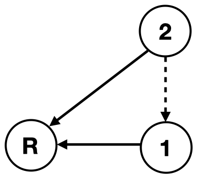
(a) 2 state variables

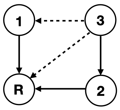
(b) 3 state variables

Figure 2: Two examples of dependence graph among reward and true state variables.

We make a few remarks. First, Condition 3 is mild. It is much weaker than requiring all the nonzero elements in $\bm{B}_{G_{\textrm{M}}}$, the sub-matrix of $\bm{B}$ formed by its rows in $G_{\textrm{M}}$, to be much larger than $n^{-1/2}\sqrt{\log p}$ (the threshold for strong signals). To elaborate, consider a simple example where the first two variables are the minimal sufficient state, both $S_{t,1}$ and $S_{t,2}$ directly influence $R_{t}$ whereas $S_{t,2}$ affects $S_{t,1}$ as well. In that case, Condition 3 requires (i) $\max_{a}|B^{(a)}_{1,p+1}|\gg\sqrt{n^{-1}\log p}$ and (ii) either $\max_{a}|B^{(a)}_{2,p+1}|\gg\sqrt{n^{-1}\log p}$ or $\max_{a}|B^{(a)}_{2,1}|\gg\sqrt{n^{-1}\log p}$. Notice that (ii) is much weaker than requiring both $\max_{a}|B^{(a)}_{2,p+1}|\gg\sqrt{n^{-1}\log p}$ and $\max_{a}|B^{(a)}_{2,1}|\gg\sqrt{n^{-1}\log p}$. This occurs essentially because there exist two directed paths from the second state variable to the reward, given by $S_{t,2}\to R_{t}$ and $S_{t,2}\to S_{t,1}\to R_{t}$, and we only require one of them to appear in the subgraph after removing edges with weak signals. Thus, we refer to this phenomenon as “the blessings of multiple paths,” which allows us to impose a weaker minimal signal strength condition. We call edges remaining in the subgraph strong edges and removed ones weak edges. Two examples are given in Figure 2, where solid lines denote strong edges, while dashed lines denote weak edges. Further interpretations are given in Lemma C.5 of the Supplemental Material and the remarks following it. Second, Condition 4 is mild as well. It is automatically satisfied when the matrix $\mathbf{E}[\mathbf{S}_{t}\mathbf{S}_{t}^{\top}\mathbb{I}(A_{t}=a)]$ possesses the restricted eigenvalue condition and the error $\mathbf{\varepsilon}_{t}$ has sub-exponential tails (see e.g., Bickel et al., 2009). It guarantees all strong signals will be detected via LASSO with probability approaching one.

Theorem 3.

Assume Conditions 3 and 4 hold. The power of SEEK using LASSO is lower bounded by

$$\textbf{Power}:=\mathbf{E}\left(\frac{|\widehat{G}\cap G_{\textrm{M}}|}{|G_{\textrm{M}}|}\right)\geq 1-O\{p^{-c_{1}}\},$$

which approaches one as $NT\rightarrow\infty$.

5.3.2 Generic Machine Learning Methods

In this section, we focus on the setting where a generic machine learning method is applied to $\widetilde{\mathcal{D}}_{k}^{(a)}$ to calculate a variable importance (VI) score for each state as well as its knockoff variable. When LASSO is employed, these VI’s correspond to the estimated regression coefficients. When the random forest algorithm is applied, it will simultaneously produce an importance measure for each variable. Alternatively, deep neural networks are applicable to produce these measures as well (Lu et al., 2018). To handle multiple outcomes, we propose to calculate the VI for each individual response variable and obtain the maximum value over all responses. Let $\textrm{VI}^{(a,k)}_{j,i}$ denote the $j$th variable’s VI with the $i$th state being the outcome. Then we can define the $W$-statistic $W_{j}^{(k)}=\max_{a\in\mathcal{A}}\max_{i}|\textrm{VI}_{j,i}^{(a,k)}|-\max_{a\in\mathcal{A}}\max_{i}|\textrm{VI}_{j+p,i}^{(a,k)}|$.

To characterize the power property, similar to Section 5.3.1, we construct a $(p+1)\times(p+1)$ matrix $\mathbf{V}^{(k)}$ whose $(j,i)$th entry equals $\max_{a}|\textrm{VI}_{j,i}^{(a,k)}|$ for $j\leq p$ and $0$ for $j=p+1$. This generates a directed graph $\mathcal{G}(\mathbf{V}^{(k)})$.

Condition 5 (Separation).

There exists a function $\gamma(n,p)$ and constant $c_{2}>0$, such that with probability of at least $1-O(p^{-c_{2}})$, and any $k\in[K]$:

1. $\max_{a\in\mathcal{A}}|\textrm{VI}_{j,i}^{(a,k)}|<\gamma(n,p)/2$ for any $j\in[2p]\backslash G_{\textrm{M}}$ and any $i\in[p+1]$;

2. the subgraph of $\mathcal{G}(\mathbf{V}^{(k)})$, by removing edges with weights smaller than $\gamma(n,p)$, identifies $G_{\textrm{M}}$.

Remark 2.

The separation assumption is mild in the sense that we do not require $\textrm{VI}_{j,i}^{(a,k)}$’s to converge to some population-level variable importance measures as the sample size increases. The first part of Condition 5 essentially upper bounds the importance of the insignificant variables whereas the second part corresponds to the signal strength condition. Similar to Condition 3, it only requires the existence of one path from the reward to each minimal sufficient state after removing edges with weak signals.

Theorem 4.

Suppose Condition 5 holds. Then the power of SEEK using general ML methods is bounded below by

$$\textbf{Power}\geq 1-O\{p^{-c_{2}}\},$$

which asymptotically increases to one as $NT\rightarrow\infty$.

6 Simulation Experiments

6.1 Experiment Design, Benchmarks, and Evaluation Metrics

In this section, we investigate the finite sample performance of SEEK via extensive simulation studies. Specifically, we consider a total of four different environments, including an autoregressive model (denoted AR) where all states follow an AR(1) model detailed in Section A of the Supplemental Material, the one specified in Section 3 which includes both autoregressive and i.i.d. states (denoted Mixed) and two environments from OpenAI Gym (Brockman et al., 2016): ‘CartPole-v0’ (denoted CP) and ‘LunarLander-v2’ (denoted LL).

In the first two environments, the action is binary. The dimensions of the minimal sufficient state $p_{0}$ and the null state $p-p_{0}$ are given by 2 and 18, respectively. The horizon is fixed at 150 whereas the number of trajectories $N$ is chosen from $\{10,20,40\}$ for the AR environment and $\{50,100,200\}$ for the Mixed environment. In the last two environments, $p_{0}$ equals 4 and 8, respectively. In addition, we manually include null variables in the state with $p$ taking values in $\{50,100,150,200\}$ which leads to a challenging high-dimensional state system, and consider both AR(1) and i.i.d. white noises for the null variables. $N$ is chosen from $\{100,200\}$, where each trajectory contains approximately 130 decision points in ‘CartPole-v0’ and 340 decision points in ‘LunarLander-v2’.

Each batch dataset is generated using $\epsilon$-greedy algorithm with $\epsilon=0.3$ as the behavior policy. The optimal policies in the first two environments have closed-form expressions. In the last two environments, CP and LL, the optimal policy is trained via a Deep Q-Network (Mnih et al., 2015) agent for CP or by a Duelling Double Deep Q-Network (Wang et al., 2016) agent for LL.

To implement SEEK, we fix the majority vote threshold $\alpha=0.5$ and the target FDR at level $q=0.1$. In the first two environments, the exponential $\beta$-mixing condition (see Condition 1) is satisfied and we apply our proposal in Section 4.2 to adaptively determine the number of splits, with $\delta$ fixed to $0.01$. In addition, because the system is linear, we apply LASSO in Step 3 of Algorithm 2 to implement SEEK. However, the last two environments are neither ergodic nor linear. As such, we fix $K$ across different simulation replications, conduct a sensitivity analysis in below to analyse the effect of $K$, and apply random forests (RFs) to implement Algorithm 2. Three benchmark methods are included, including two one-step approaches (see Section 3) that conduct variable selection via LASSO and RF, denoted by VS-LASSO and VS-RF, respectively, as well as the sparse feature selection (SFS) method by Hao et al. (2021) based on LASSO. For the first two linear environments, we only report the results based on SEEK, VS-LASSO, and SFS whereas, for the last two nonlinear environments, we report results based on SEEK, VS-RF, and SFS.

The aforementioned methods are evaluated by the following criteria: FDR/mFDR, false positive rate (FPR, the percentage of falsely selected variables), true positive rate (TPR, the percentage of correctly selected variables), and the value of the estimated optimal policy based on the selected state variables using the same batch data. To compute the value, we first apply FQI to the reduced MDP with the selected state to estimate the optimal policy and then apply the Monte Carlo method for policy value evaluation. When implementing FQI, we employ the multilayer perceptron regressor implementation of Pedregosa et al. (2011) to perform supervised learning. Information about hyper-parameters is given in Tables A.1 and A.2 of the Supplemental Materials.

Table 2: Performances of SEEK and benchmark methods in the AR environment, aggregated over 100 simulation runs.

	SEEK				SFS		VS-LASSO
$N$	10	20	40	10	20	40	10	20	40
$T$	150	150	150	150	150	150	150	150	150
$K$	19.60	24.62	29.28	/	/	/	19.60	24.62	29.28
mFDR	0.00	0.00	0.00	0.02	0.01	0.02	0.60	0.60	0.60
FDR	0.00	0.00	0.00	0.07	0.03	0.06	0.90	0.90	0.90
FPR	0.00	0.00	0.00	0.02	0.01	0.02	1.00	1.00	1.00
TPR	0.96	1.00	1.00	1.00	1.00	1.00	1.00	1.00	1.00
Value	1.98	2.07	2.08	2.02	2.06	2.07	1.49	1.77	1.90

Table 3: Performances of SEEK and benchmark methods in the Mixed environment, aggregated over 100 simulation runs.

	SEEK			SFS			VS-LASSO
$N$	50	100	200	50	100	200	50	100	200
$T$	150	150	150	150	150	150	150	150	150
$K$	3.22	4.16	4.56	/	/	/	3.22	4.16	4.56
mFDR	0.04	0.01	0.01	0.03	0.02	0.01	0.00	0.00	0.00
FDR	0.12	0.04	0.05	0.14	0.09	0.04	0.00	0.00	0.00
FPR	0.04	0.01	0.01	0.02	0.02	0.01	0.00	0.00	0.00
TPR	0.71	0.98	1.00	0.51	0.53	0.54	0.50	0.50	0.50
Value	2.17	2.19	2.19	2.17	2.19	2.19	2.17	2.19	2.19

Table 4: Performances of SEEK for different $K$ in the AR environment, aggregated over 100 simulation runs.

	Selected K			K=5			K=10			K=20			K=40
N	10	20	40	10	20	40	10	20	40	10	20	40	10	20	40
T	150	150	150	150	150	150	150	150	150	150	150	150	150	150	150
K	19.60	24.62	29.28	/	/	/	/	/	/	/	/	/	/	/	/
mFDR	0.00	0.00	0.00	0.01	0.01	0.01	0.00	0.00	0.00	0.00	0.00	0.00	0.03	0.00	0.00
FDR	0.00	0.00	0.00	0.03	0.04	0.03	0.01	0.02	0.00	0.00	0.00	0.00	0.12	0.00	0.00
FPR	0.00	0.00	0.00	0.00	0.01	0.00	0.00	0.00	0.00	0.00	0.00	0.00	0.02	0.00	0.00
TPR	0.96	1.00	1.00	1.00	1.00	1.00	1.00	1.00	1.00	0.89	1.00	1.00	1.00	0.98	1.00
Value	1.98	2.07	2.08	2.03	2.06	2.08	2.03	2.06	2.08	1.87	2.07	2.08	2.01	2.04	2.08

Table 5: Performances of SEEK with different $K$ in the Mixed environment, aggregated over 100 simulation runs.

	Selected K			K=5			K=10			K=20			K=40
N	50	100	200	50	100	200	50	100	200	50	100	200	50	100	200
T	150	150	150	150	150	150	150	150	150	150	150	150	150	150	150
K	3.22	4.16	4.56	/	/	/	/	/	/	/	/	/	/	/	/
mFDR	0.04	0.01	0.01	0.01	0.00	0.00	0.00	0.00	0.00	0.00	0.00	0.00	0.00	0.00	0.00
FDR	0.12	0.04	0.05	0.03	0.02	0.01	0.00	0.00	0.00	0.00	0.00	0.00	0.00	0.00	0.00
FPR	0.04	0.01	0.01	0.00	0.00	0.00	0.00	0.00	0.00	0.00	0.00	0.00	0.00	0.00	0.00
TPR	0.71	0.98	1.00	0.50	0.95	1.00	0.50	0.50	0.98	0.50	0.50	0.50	0.50	0.50	0.50
Value	2.17	2.19	2.19	2.17	2.19	2.19	2.17	2.19	2.19	2.17	2.19	2.19	2.17	2.19	2.19

6.2 Results

Results are reported in Tables 2 & 3 as well as Figures 3 & 4 respectively. We summarize our findings as follows. First, the proposed SEEK algorithm outperforms other baseline methods, with FDRs close to zero and TPRs close to one in almost all cases. In addition, it can be seen from Tables 2 & 3 and Figure 3 that the resulting policies based on the selected state variables achieve the highest values. This demonstrates the importance of variable selection to RL. Second, the one-step variable selection method fails with high FDR when the null variables follow an AR model and does not select enough variables in the Mixed environment. Third, SFS has low power in the Mixed environment and fails to control FDR in the LL environment. As noted previously, this is because SFS requires linear function approximation and cannot handle complex nonlinear systems. These results align with our theoretical findings, demonstrating the advantage of the proposed SEEK algorithm.

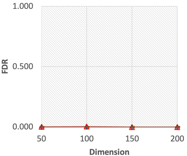
(a) $N=100$, i.i.d.

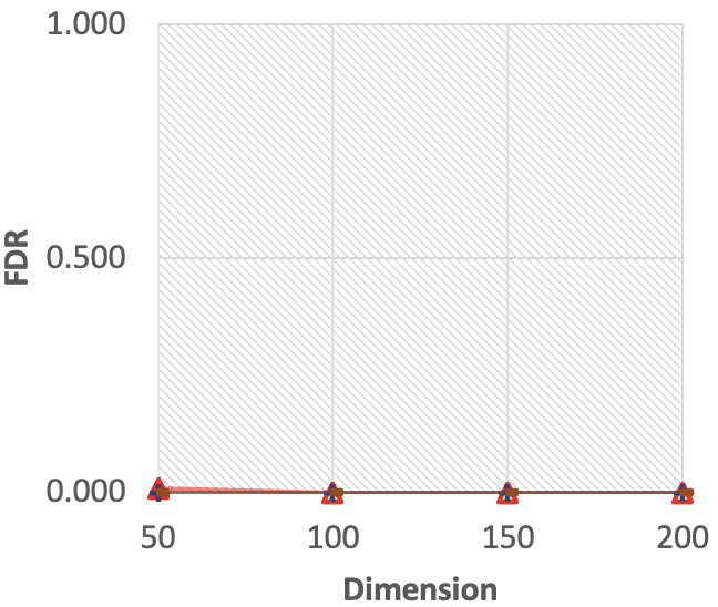
(b) $N=200$, i.i.d.

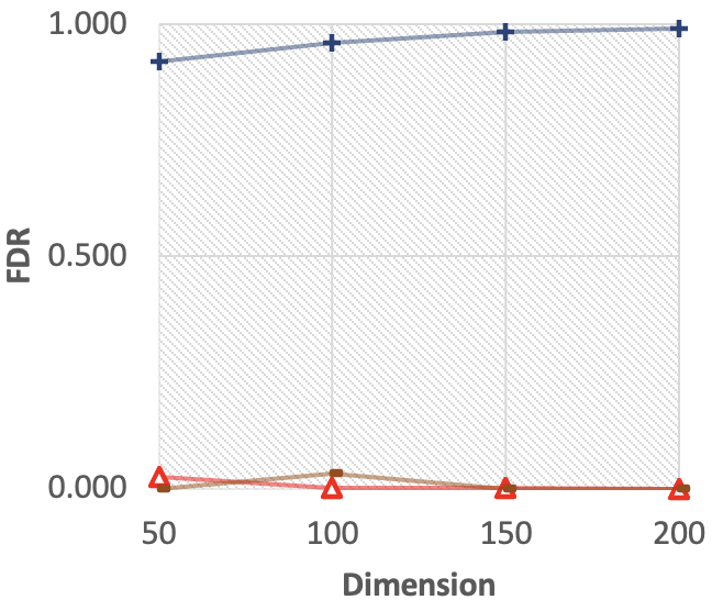
(c) $N=100$, AR noise.

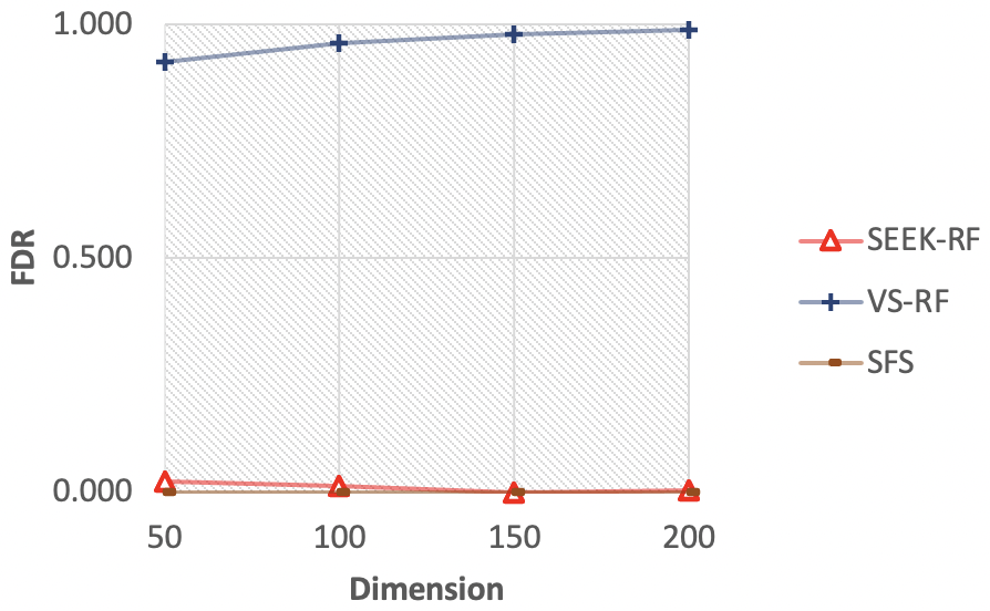
(d) $N=200$, AR noise.

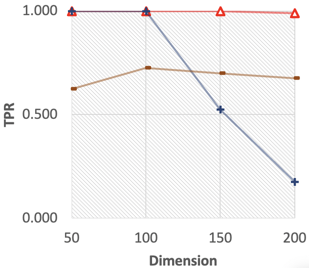
(e) $N=100$, i.i.d.

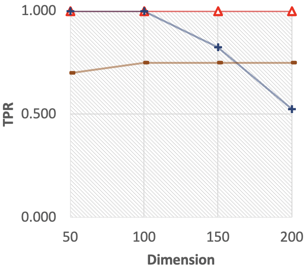
(f) $N=200$, i.i.d.

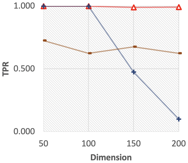
(g) $N=100$, AR noise.

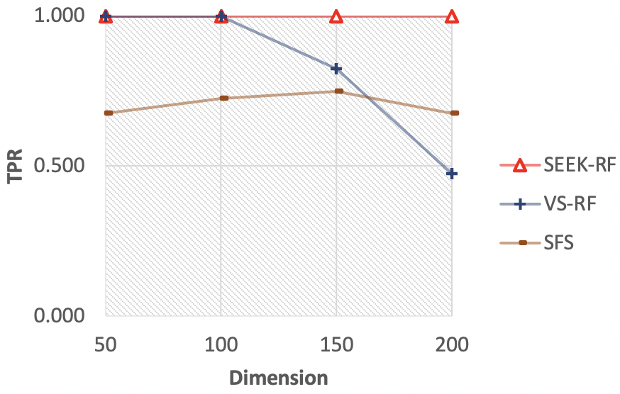
(h) $N=200$, AR noise.

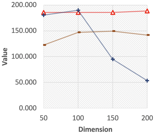
(i) $N=100$, i.i.d.

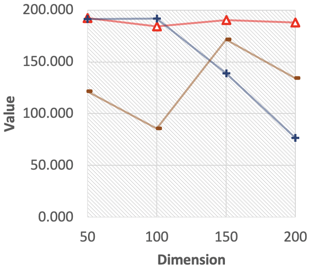
(j) $N=200$, i.i.d.

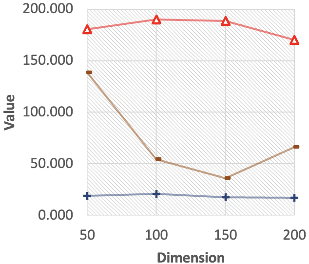
(k) $N=100$, AR noise.

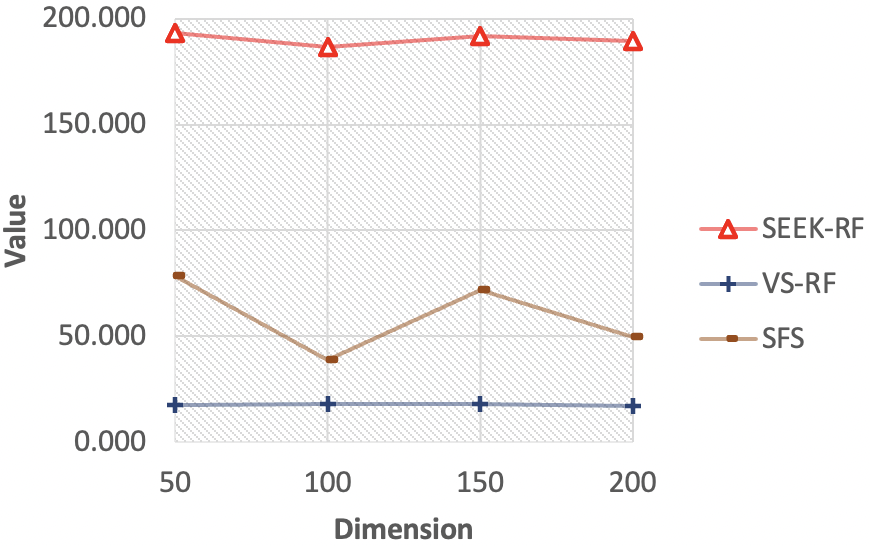
(l) $N=200$, AR noise.

Figure 3: Comparison results of the false discovery rate (FDR), the true positive rate (TPR), and the value based on SEEK-RF, VS-RF, and SFS under ‘CartPole-v0’.

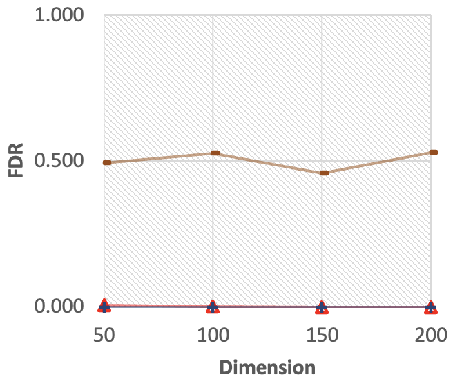
(a) $N=100$, i.i.d.

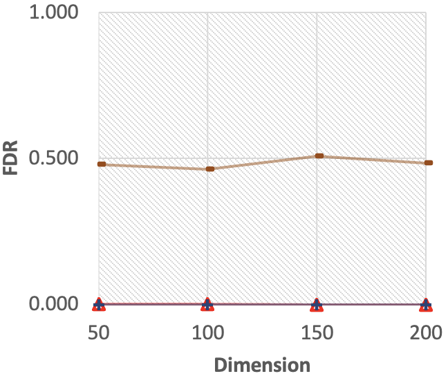
(b) $N=200$, i.i.d.

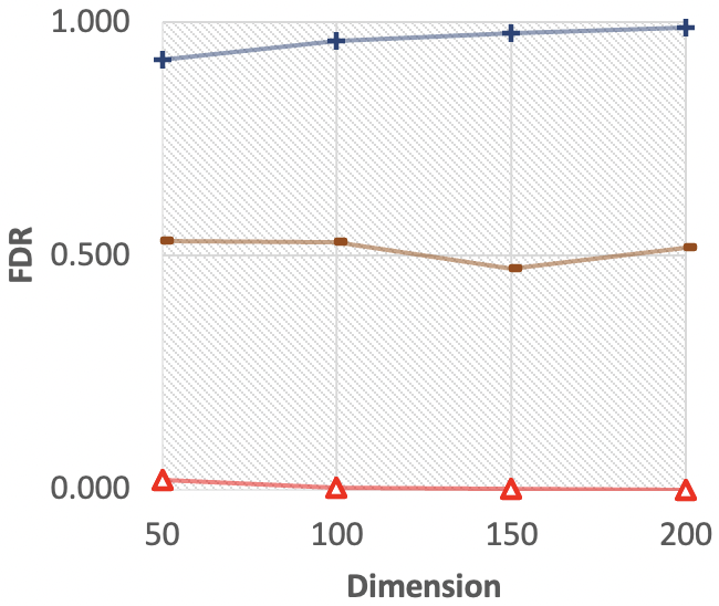
(c) $N=100$, AR noise.

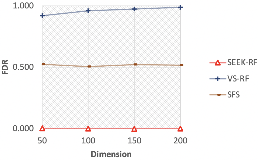
(d) $N=200$, AR noise.

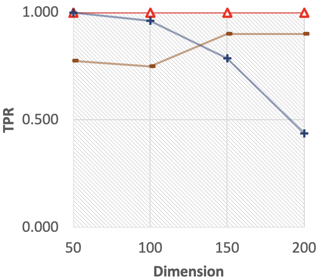
(e) $N=100$, i.i.d.

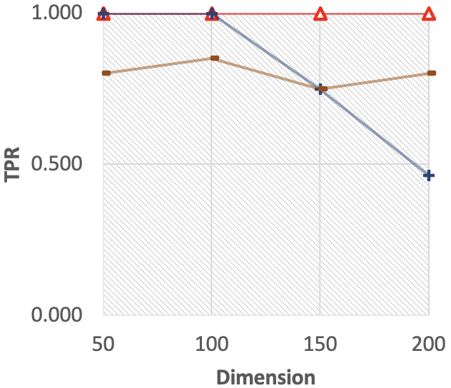
(f) $N=200$, i.i.d.

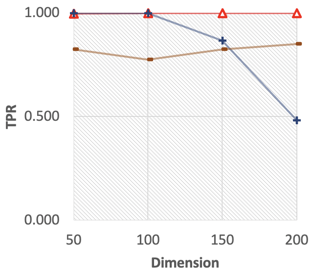
(g) $N=100$, AR noise.

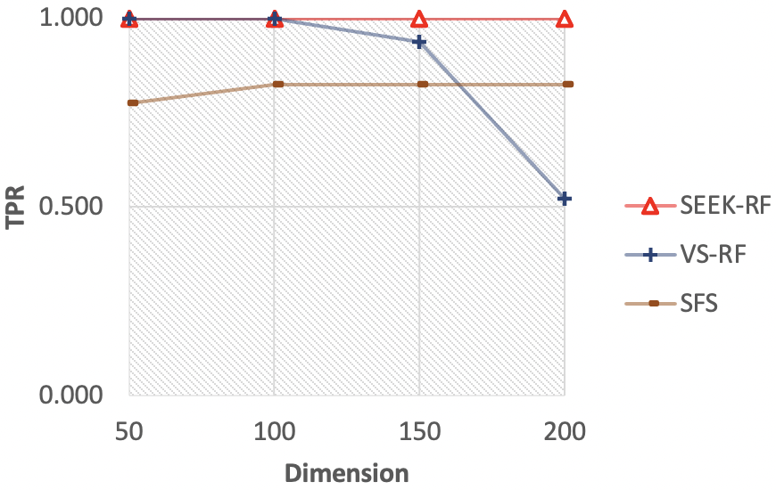
(h) $N=200$, AR noise.

Figure 4: Comparison results of the false discovery rate (FDR) and the true positive rate (TPR) based on SEEK-RF, VS-RF, and SFS under ‘LunarLander-v2’, aggregated over 100 runs.

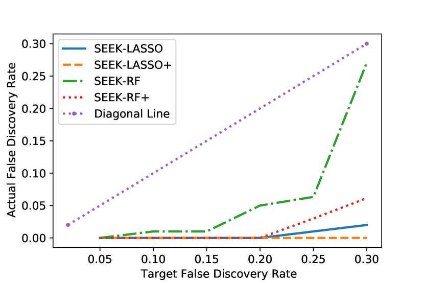
(a) $K=\log(NT)$

(b) $K=1.5\log(NT)$

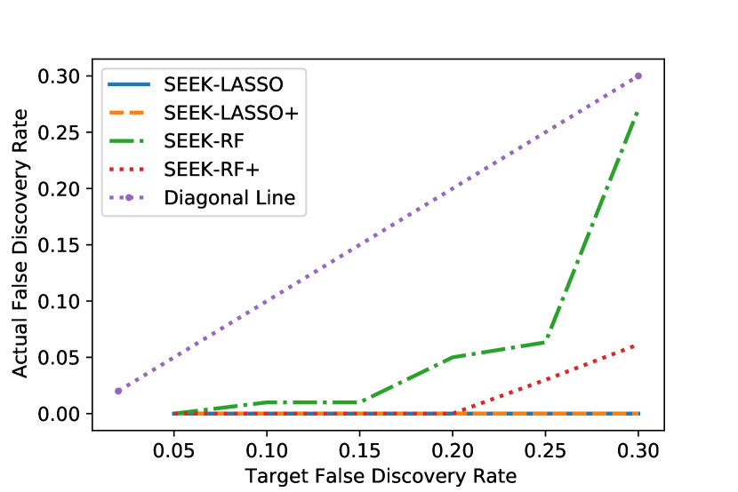
(c) $K=2\log(NT)$

Figure 5: Results of the FDR using the proposed SEEK methods under ‘CartPole-v0’ with $N=100$, $p=100$, $\alpha=0.5$, and AR(1) noises. All the results are aggregated over 20 runs.

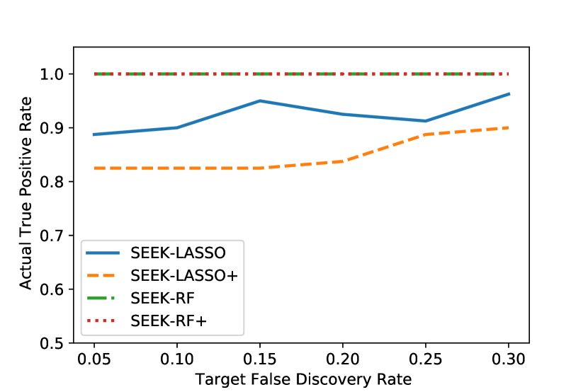
(a) $K=\log(NT)$

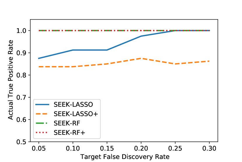
(b) $K=1.5\log(NT)$

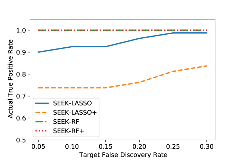
(c) $K=2\log(NT)$

Figure 6: Results of the TPR using the proposed SEEK methods under ‘CartPole-v0’ with $N=100$, $p=100$, $\alpha=0.5$, and AR(1) noises. All the results are aggregated over 20 runs.

To investigate the proposed $K$-selection algorithm in Section 4.2, we conduct another analysis that applies SEEK to the first two environments with $K$ fixed to $5,10,20,40$ and compares the results against those obtained based on SEEK with adaptively selected $K$. See Tables 4 & 5for details. It can be seen from Table 5 that mFDR, FDR, and TPR depend on the specification of $K$. In particular, when $K$ is moderately large (e.g., 10 or 20), the TPR is reduced to half whereas the mFDR, FDR, and FPR are exactly equal to zero. On the contrary, the proposed $K$-selection algorithm tends to select a small value of $K$ in the Mixed environment, achieving a better balance between (m)FDR/FPR and TPR.

In addition, we conduct a sensitivity analysis to test the robustness of four SEEK methods (SEEK-LASSO, SEEK-RF, SEEK-LASSO+, and SEEK-RF+, where SEEK-X+ refers to the SEEK-X algorithm with knockoffs+ for variable selection) to different choices of $K$ and $q$, when the $\beta$-mixing assumption does not hold. We focus on the ‘CartPole-v0’ environment with $N=100$, $p=100$, and AR(1) noise, set $K=k_{0}\log(NT)$ with $k_{0}\in\{1,1.5,2\}$, choose $q\in(0,0.3]$ for the FDR control, and plot the corresponding FDRs and TPRs in Figures 5 and 6 respectively. It can be seen that our method controls the FDR for any $K$ and $q$. In addition, the performance is not overly sensitive to the choice of $K$.

7 Real Data Analysis

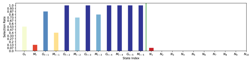
(a) Results under SEEK.

(b) Results under SFS.

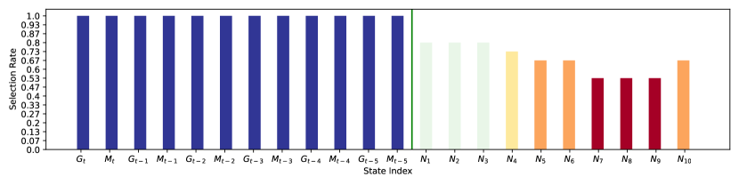
(c) Results under VS-LASSO.

Figure 7: Results of real data analysis based on SEEK, VS-LASSO, and SFS.

In this section, we apply SEEK to the OhioT1DM dataset (Marling & Bunescu, 2020) which contains data from 6 patients with type-I diabetes. For each patient, their glucose levels and self-reported meals are continuously measured over 8 weeks. These variables can be used to construct data-driven decision rules to determine whether a patient needs insulin injections to improve their health (Luckett et al., 2019; Shi et al., 2022; Zhou et al., 2022).

To analyze this data, we divide the eight weeks into one-hour intervals and compute the average glucose level $G_{t}$ and the average carbohydrate estimate for the meal $M_{t}$ over each one-hour interval $(t-1,t]$. Previous studies found these variables do not satisfy the Markov assumption (see e.g., Shi et al., 2020). This motivates us to construct the state $S_{t}$ by including both the current observations $G_{t}$, $M_{t}$ as well as the past measurements within 5 hours, i.e., $G_{t-i}$ and $M_{t-i}$ for $i=1,2,3,4,5$. We also manually include 10 null variables (denoted by $N_{1},\cdots,N_{10}$) in the state, each following an AR(1) model. The action $A_{t}$ is binary, indicating whether the patient injected the insulin or not in the last hour.

We next apply SEEK, VS-LASSO, and SFS to 4 out of 6 data trajectories for variable selection, iterate this procedure for all $\binom{6}{4}=15$ combinations, compute the percentage of each state variable being selected and report the results in Figure 7. It can be seen that (i) VS-LASSO has a high FDP with each of the null variables being selected at least $50\%$ of the time; (ii) SFS fails to identify the glucose levels and carbohydrate estimates as significant variables, suffering from a low TPR; (iii) SEEK rarely selects null variables and has a high success rate in selecting glucose levels and carbohydrate estimates.

8 Discussion

There are several potential topics for further research. In this paper, we assume the environment is time-homogeneous. It would be interesting to extend the proposed ideas to handle non-stationary environments where the set of significant variables evolves with time as well. Another extension is to consider variable selection in a partially observed MDP (POMDP); in this case, we may want to apply SEEK to the belief state MDP. Finally, it is worthwhile to consider other (non-knockoff) variable selection methods to identify the minimal sufficient state in sequential decision making.

Appendix A Additional Numerical Details

In this section, we provide additional numerical configurations, especially the data generating processes and hyper-parameters information.

The AR environment in Section 6 is generated as follows. Each state is generated according to: $S_{t+1,j}=0.9S_{t,j}A_{t}+0.09S_{t,j}(1-A_{t})+N(0,1)$ for any $t$ and $j$. The reward is given by $R_{t}=A_{t}(S_{t,1}+S_{t,2})+N(0,1)$ for any $t$. In the real data analysis, each of the null variables follows an AR(1) model, given by $S_{t+1,j}=0.5S_{t,j}+N(0,1)$.

In our implementation, we apply LASSO and random forest to compute the $W$-statistics and summarize their hyper-parameters information in Tables A.1 and A.2, respectively.

Table A.1: Hyper-parameters information for LASSO.

Hyper-parameters	Values
Penalty term $\lambda$ selection criterion	Bayesian information criterion (BIC)
Penalty term $\lambda$ selection range	$[\exp(-20),\exp(-8)]$

Table A.2: Hyper-parameters information for random forest.

Hyper-parameters	Values
Number of trees in the forest	$NT/K/30$
Maximum depth of the tree	4
Number of variables for the best split	$\sqrt{p}$
Others	Default values in python package ‘sklearn’

Appendix B Additional Algorithmic Details

In this section, we give more details about some major steps of the proposed algorithm.

B.1 Action-based Sub-grouping

We first provide the intuition behind the sub-grouping. Different from the classical supervised learning setting, although both the state and action contribute to the reward function and system transition, we only care about the selection of state variables. Let $I_{s},I_{a}$ denote the index sets of states and actions respectively. Our goal is to select a subset of $I_{s}$ (denoted by $G$), treating the variables in $I_{a}$ as significant variables. We call this a partial selection problem.

Under partial selection, the knockoffs $\tilde{\mathbf{S}}$ in our setting should satisfy the two properties mentioned in Section 2 conditional on actions. We next discuss two approaches to meet these properties. To motivate the first approach, we notice that according to the exchangeability property,

$$[\mathbf{S},\widetilde{\mathbf{S}},\mathbf{a}]_{\text{swap}(B)}\overset{d}{=}[\mathbf{S},\widetilde{\mathbf{S}},\mathbf{a}]$$

for any index subset $B\in\{1,...,p\}$. This leads to the exact construction method (see Candès et al. 2018, Algorithm 1), which iteratively samples the knockoff variable $\widetilde{S}_{j}$ for $j=1$ till $p$, row by row. However, such a method is computationally infeasible in moderate dimensional settings.

The second method is to construct knockoffs that approximately satisfy the exchangeability property conditional on each distinct value of actions, as we adopt in Algorithm 2. We detail this method in the next subsection.

B.2 Knockoffs Construction

We begin with some notations. For each $a\in\mathcal{A}=\{1,2,...,m\}$, let $\mathcal{D}_{k}^{(a)}$ denote the data subset $\left\{(\mathbf{S}_{i},A_{i},\mathbf{Y}_{i})\in\mathcal{D}_{k}:A_{i}=a\right\}$, with size $n_{k,a}$. Notice that $\sum_{a}n_{k,a}=NT/K$. Recall that $\mathbf{Y}_{i}$ represents either an immediate reward, or some significant states.

For ease of representation below, we write $\mathcal{D}_{k}$ in the matrix form, e.g.,

$$\mathcal{D}_{k}=[\mathbf{s}_{k},\mathbf{a}_{k},\mathbf{y}_{k},\mathbf{s}_{k}^{\prime}]$$

with $\mathbf{s}_{k},\mathbf{s}_{k}^{\prime}\in\mathbb{R}^{(NT/K)\times p},\mathbf{a}_{k},\mathbf{r}_{k}\in\mathbb{R}^{NT/K}$ and each row of $\mathcal{D}_{k}$ corresponds to one transition tuple. Similarly, for each $a\in\mathcal{A}$, we have

$$\mathcal{D}_{k}^{(a)}=[\mathbf{s}_{k}^{(a)},\mathbf{y}_{k}^{(a)},\mathbf{s}_{k}^{\prime(a)}]$$

with $\mathbf{s}_{k}^{(a)},\mathbf{s}_{k}^{\prime(a)}\in\mathbb{R}^{n_{k,a}\times p},\mathbf{y}_{k}^{(a)}\in\mathbb{R}^{n_{k,a}}$.

Remark 3.

We briefly discuss these notations. Upper and lower case letters refer to random variables and data realizations respectively, whereas boldface letters denote vectors or matrices. The subscript $k$ and/or superscript $(a)$ is included to highlight the data subset $\mathcal{D}_{k}^{(a)}$ obtained by data splitting and/or action sub-grouping. For example, $\mathbf{s}_{k}^{(a)}$ denotes the states in the data subset $\mathcal{D}_{k}^{(a)}$. Finally, $S_{k,j}$ denotes the $j$th element of $\mathbf{S}_{k}$.

On each $\mathcal{D}_{k}^{(a)}$, we aim to construct knockoffs so that

$$[\mathbf{S}_{k}^{(a)}~{}\widetilde{\mathbf{S}}_{k}^{(a)}]_{\text{swap}(B)}\overset{d}{=}[\mathbf{S}_{k}^{(a)}~{}\widetilde{\mathbf{S}}_{k}^{(a)}].$$

We discuss two concrete proposals below to construct knockoffs. Meanwhile, other proposals are equally applicable as long as they meet the exchangeability assumption.

B.2.1 Second-order Machine (Gaussian Sampling)

Suppose $\mathbf{S}_{k}^{(a)}$ follows a multivariate normal distribution with mean zero (we normalized the state in practice to meet this assumption), covariance matrix $\Sigma_{k}^{(a)}$. In order to satisfy the exchangeability assumption, it suffices to construct $\widetilde{\mathbf{S}}_{k}^{(a)}$ according to the following,

$$\tilde{\mathbf{S}}_{k}^{(a)}|\mathbf{S}_{k}^{(a)}\overset{d}{=}\mathcal{N}(\mathbf{\mu}_{k}^{(a)},V_{k}^{(a)}),$$

where $(\mathbf{\mu}_{k}^{(a)},V_{k}^{(a)})$ is given by

$$\mathbf{\mu}_{k}^{(a)} =\mathbf{S}_{k}^{(a)}-\mathbf{S}_{k}^{(a)}(\Sigma_{k}^{(a)})^{-1}\text{diag}\{\mathbf{d}_{k}^{(a)}\},$$

$$V_{k}^{(a)} =2\text{diag}\{\mathbf{d}_{k}^{(a)}\}-\text{diag}\{\mathbf{d}_{k}^{(a)}\}(\Sigma_{k}^{(a)})^{-1}\text{diag}\{\mathbf{d}_{k}^{(a)}\}.$$

Remark 4.

As proven in Appendix C.2, such a construction leads to the following joint distribution:

$$(\mathbf{S}_{k}^{(a)},\widetilde{\mathbf{S}}_{k}^{(a)})\sim\mathcal{N}(\mathbf{0},\mathbf{U}_{k}^{(a)}),\mathbf{U}_{k}^{(a)}=\begin{bmatrix}\Sigma_{k}^{(a)}&\Sigma_{k}^{(a)}-\text{diag}\{\mathbf{d}_{k}^{(a)}\}\\ \Sigma_{k}^{(a)}-\text{diag}\{\mathbf{d}_{k}^{(a)}\}&\Sigma_{k}^{(a)}\end{bmatrix}\geq\mathbf{0}.$$

The diagonal elements $\mathbf{d}_{k}^{(a)}\in\mathbb{R}^{p}$ shall be chosen such that $\mathbf{U}_{k}^{(a)}$ is positive semidefinite with all entries being nonnegative. On the other hand, each entry in $\mathbf{d}_{k}^{(a)}$ should be as large as possible to reduce the correlation between $S_{k}^{(a)}$ and $\widetilde{S}_{k}^{(a)}$. One could adopt the approximate semidefinite program developed in Candès et al. (2018) to determine $\mathbf{d}_{k}^{(a)}$.

Remark 5.

The above construction allows the first two moments of $\widetilde{S}_{k}^{(a)}$ to match those of $S_{k}^{(a)}$. Thus, we refer to this method as a second-order (sampling) machine. In practice, it works well even without the normality assumption.

B.2.2 Deep Sampling

Alternatively, we can construct the knockoff variables by matching higher order moments using deep neural networks (see e.g., Romano et al. 2020). The basic idea is to construct an objective function $J(S_{k}^{(a)},\widetilde{S}_{k}^{(a)})$ which measures the discrepancy between $S_{k}^{(a)}$ and $\widetilde{S}_{k}^{(a)}$ in distribution and apply a deep generative model to minimizes this objective function.

B.3 Feature Importance Statistics

Conditional on $A=a$, each state variable $S_{k,j}^{(a)}$ (and its knockoff $\widetilde{S}_{k,j}^{(a)}$) in the augmented data subset $\widetilde{\mathcal{D}}_{k}^{(a)}$ (by augmenting $\mathcal{D}_{k}^{(a)}$ with $\tilde{s}_{k}^{(a)}$) has its own feature importance statistics, denoted by $Z_{k,j}^{(a)}$ (respectively, $\widetilde{Z}_{k,j}^{(a)}$). To aggregate them over different actions, we define

$$Z_{k,j}=\max\limits_{a}Z_{k,j}^{(a)},\qquad\widetilde{Z}_{k,j}=\max\limits_{a}\widetilde{Z}_{k,j}^{(a)}.$$

Alternative aggregation methods can be considered as well. After that, we use an anti-symmetric function $f$ to calculate the $W$-statistics. In our implementation, we set $f(u,v)$ to $u-v$, and show that the resulting $W$-statistic satisfies the flip-sign property in Lemma C.3 of Appendix C.2. We next discuss the construction of $Z_{k,j}^{(a)}$ (and $\widetilde{Z}_{k,j}^{(a)}$) based on three machine learning methods.

B.3.1 Penalized Linear Regression

The first approach is to perform penalized linear regressions via LASSO (Tibshirani 1996), SCAD (Fan & Li 2001), or MCP (Zhang 2010) to the data subset $\mathcal{D}_{k}^{(a)}$ to obtain the feature importance statistics. For each $a$, denote the estimated coefficients by

$$\widehat{\mathbf{B}}^{(a,k)}=[\widehat{\mathbf{B}}^{(a,k)}_{1},...,\widehat{\mathbf{B}}^{(a,k)}_{p+1}],$$

where $\widehat{\mathbf{B}}^{(a,k)}_{i}\in\mathbb{R}^{2p}$ is the coefficient vector for $i$-th response variable, and the $j$-th row in $\widehat{\mathbf{B}}^{(a,k)}$ corresponds to all the coefficients with the $j$-th state variable, i.e. $S_{k,j}^{(a)}$ if $j\leq p$, $\widetilde{S}_{k,j-p}^{(a)}$ if $p+1\leq j\leq 2p$. Then the feature importance $Z_{k,j}^{(a)}$ and $\widetilde{Z}_{k,j}^{(a)}$ can be measured by

$$Z_{k,j}^{(a)} =\max_{i\in I}|\widehat{B}^{(a,k)}_{j,i}|,\qquad 1\leq j\leq p,$$

$$\widetilde{Z}_{k,j}^{(a)} =\max_{i\in I}|\widehat{B}^{(a,k)}_{j+p,i}|,\qquad 1\leq j\leq p.$$

where $I$ denoted the index set for all the current response variables.

B.3.2 Random Forest

For each $a\in\mathcal{A}$, we set $Z_{k,j}^{(a)}$ and $\widetilde{Z}_{k,j}^{(a)}$ to the corresponding variable importance score of the predictors $\mathbf{S}_{k,j}^{(a)}$ and $\widetilde{\mathbf{S}}_{k,j}^{(a)}$ output by the random forest algorithm.

B.3.3 Deep Neural Network

Alternatively, we can fit a deep neural network to the data, and combine the coefficients in each layer to calculate the variable importance scores $Z_{k,j}^{(a)}$ and $\widetilde{Z}_{k,j}^{(a)}$ (see Lu et al. 2018).

B.4 Additional Details in the K-Selection Algorithm

We employ importance sampling to evaluate the integral in (3) when estimating the $\beta$-mixing coefficients. To simplify the calculation, we assume $\pi_{b}$ and $\pi_{b}^{\prime}$ are approximately the same so that $\beta(k)$ can be approximated by $\int_{s,s^{\prime}}|f(s)f(s^{\prime})-f_{k}(s,s^{\prime})|/2$. A naive method is to uniformly sample $(S_{i},S_{i}^{\prime})$ over the product space $\mathcal{S}\times\mathcal{S}$ and estimate $\beta(k)$ by

$$\frac{|\mathcal{S}|^{2}}{2M}\sum_{i=1}^{M}|\widehat{f}(S_{i})\widehat{f}(S_{i}^{\prime})-\widehat{f}_{k}(S_{i},S_{i}^{\prime})|,$$ (B.1)

where $\widehat{f}$ and $\widehat{f}_{k}$ denote the corresponding estimators for $f$ and $f_{k}$, respectively. However, this method requires the state space to be bounded. In addition, the resulting estimator may suffer from a large variance when the area of the state space is large.

In our implementation, we propose to sample $(S_{i},S_{i}^{\prime})$ according to a mixture distribution $1/2[\widehat{f}(S_{i})\widehat{f}(S_{i}^{\prime})+\widehat{f}_{k}(S_{i},S_{i}^{\prime})]$. This yields the following estimator

$$\frac{1}{M}\sum_{i=1}^{M}\frac{|\widehat{f}(S_{i})\widehat{f}(S_{i}^{\prime})-\widehat{f}_{k}(S_{i},S_{i}^{\prime})|}{|\widehat{f}(S_{i})\widehat{f}(S_{i}^{\prime})+\widehat{f}_{k}(S_{i},S_{i}^{\prime})|}.$$

Different from (B.1), the above importance sampling ratio is strictly smaller than $1$, reducing the variance of the resulting estimator. When $\widehat{f}$ and $\widehat{f}_{k}$ are consistent, it can be shown that its variance is upper bounded by $\beta(k)/M$ asymptotically.

Appendix C Proofs

C.1 Proofs of Propositions

C.1.1 Proof of Proposition 1

Under the MDP assumption, the optimal policy is greedy with respect to the optimal $Q$-function, denoted by $Q^{\ast}$ (Puterman 2014, Section 6). By the Bellman optimality equation, we have

$$Q^{\ast}(\mathbf{S},A) =\mathbf{E}\left[R+\gamma\max\limits_{a\in\mathcal{A}}Q^{\ast}(\mathbf{S}^{\prime},a)|\mathbf{S},A\right]$$

$$=\mathbf{E}\left[R|\mathbf{S},A\right]+\mathbf{E}\left[\gamma\max\limits_{a\in\mathcal{A}}Q^{\ast}(\mathbf{S}^{\prime},a)|\mathbf{S},A\right],$$

almost surely. Next, according to the definition of sufficient state, we notice that the two conditional expectations in the second line depend on the state only through $\mathbf{S}_{G}$. As such, $Q^{*}$ as well as the optimal policy depend on the state only through $\mathbf{S}_{G}$.

C.1.2 Proof of Proposition 2

Since $\mathcal{M}$ is an MDP, it must satisfy the following Markov properties
1. (Markov property for the next state) For any $t\geq 0$,

$$\mathbb{P}(\mathbf{S}_{t+1}|\{\mathbf{S}_{j},A_{j},R_{j}\}_{0\leq j<t},\mathbf{S}_{t},A_{t})=\mathbb{P}(\mathbf{S}_{t+1,}|\mathbf{S}_{t},A_{t})$$

2. (Markov property for the reward) For any $t\geq 0$,

$$\mathbb{P}(R_{t}|\{\mathbf{S}_{j},A_{j},R_{j}\}_{0\leq j<t},\mathbf{S}_{t},A_{t})=\mathbb{P}(R_{t}|\mathbf{S}_{t},A_{t})$$

To prove Proposition 2, we aim to show the reduced data generating process based on the sufficient state satisfies such two Markov properties as well. To save space, we only show the Markov property holds for the next state, i.e., for any $t\geq 0$,

$$\mathbb{P}(\mathbf{S}_{t+1,G}|\{\mathbf{S}_{j,G},A_{j},R_{j}\}_{0\leq j<t},\mathbf{S}_{t,G},A_{t})=\mathbb{P}(\mathbf{S}_{t+1,G}|\mathbf{S}_{t,G},A_{t}).$$

This is equivalent to require

$$\mathbf{S}_{t+1,G}\perp\!\!\!\perp\{\mathbf{S}_{j,G},A_{j},R_{j}\}_{0\leq j<t}|\mathbf{S}_{t,G},A_{t}.$$

To prove the conditional independence, we first notice that, it follows from the Markov property of the full model $\mathcal{M}$ that

$$\mathbf{S}_{t+1,G}\perp\!\!\!\perp\{\mathbf{S}_{j,G},\mathbf{S}_{j,G^{c}},A_{j},R_{j}\}_{0\leq j<t}|\mathbf{S}_{t,G},\mathbf{S}_{t,G^{c}},A_{t}.$$

Then by the decomposition rule of conditional independence,

$$\mathbf{S}_{t+1,G}\perp\!\!\!\perp\{\mathbf{S}_{j,G},A_{j},R_{j}\}_{0\leq j<t}|\mathbf{S}_{t,G},\mathbf{S}_{t,G^{c}},A_{t}$$

On the other hand, by the definition of sufficient state, we have that

$$\mathbf{S}_{t+1,G}\perp\!\!\!\perp\mathbf{S}_{t,G^{c}}|\mathbf{S}_{t,G},A_{t}.$$

Finally, combining the above two observations with the contraction rule of conditional independence, we have that

$$\mathbf{S}_{t+1,G}\perp\!\!\!\perp\{\mathbf{S}_{j,G},A_{j},R_{j}\}_{0\leq j<t},\mathbf{S}_{t,G^{c}}|\mathbf{S}_{t,G},A_{t}$$

Again applying the decomposition rule yields the desired Markov property. Especially, due to the time-homogeneity of $\mathcal{M}$, the reduced process is also time-homogeneous.

C.1.3 Proof of Proposition 3 and 4

Part 1 of the proof of Proposition 3 (existence). Denote the set of all index sets for sufficient state as $\mathcal{F}_{\text{sf}}$. First we know from the definition, $[p]\in\mathcal{F}_{\text{sf}}$, meaning that $\mathcal{F}_{\text{sf}}$ is nonempty. In addition, for any $G_{1},G_{2}\in\mathcal{F}_{\text{sf}}$, we can define the order $\leq_{\text{sf}}$ by $G_{1}\leq_{\text{sf}}G_{2}$ iff $|G_{1}|\leq|G_{2}|$. Then we can see $\leq_{\text{sf}}$ is a total order on $\mathcal{F}_{\text{sf}}$ with cardinality of elements lower bounded by $0$. Then the minimal sufficient state defined by

$$G^{\ast}=\operatorname{argmin}\limits_{G\in\mathcal{F}_{\text{sf}}}|G|$$

always exists.

If we further assume the strict positivity of the transition kernel, $G^{\ast}$ is unique, as shown below.

Part 2 of the proof of Proposition 3 (uniqueness) and proof of Proposition 4. We first discuss the 3 methods one by one to prove Proposition 4.

Reward-only approach: The toy example described in Section 3 demonstrates the insufficiency of the state selected by the reward-only approach. First, we show $\mathbf{S}_{G_{M}}=\mathbf{S}_{\{1,2\}}$ is a sufficient state. Due to the fact only $S_{t,1}$ contributes to reward, we have for any $t\geq 0$ that

$$R_{t}\perp\!\!\!\perp\mathbf{S}_{t,\{1\}^{c}}|(S_{t,\{1\}},A_{t})$$

According to the weak union rule of conditional independence, we have that

$$R_{t}\perp\!\!\!\perp\mathbf{S}_{t,G_{M}^{c}}|(\mathbf{S}_{t,G_{M}},A_{t})$$

In addition, since the state transition in the first two dimensions only depend on themselves, we have that

$$\mathbf{S}_{t+1,G_{M}}\perp\!\!\!\perp\mathbf{S}_{t,G_{M}^{c}}|(\mathbf{S}_{t,G_{M}},A_{t}).$$

This implies that $\mathbf{S}_{G_{M}}$ is a sufficient state. Furthermore, we notice for any index set $G$, if $1\notin G$, then Markov property for the reward will be violated. If $2\notin G$, the Markov property for the next state will be violated. Then for any $G\in\mathcal{F}_{\text{sf}}$, we must have $1,2\in G$. This leads to our conclusion that $\mathbf{S}_{G_{M}}$ is the unique minimal sufficient state in this scenario.

As for the reward-only approach, it only selects the first state variable and is thus insufficient.

One-step approach: Any such method would select a subset $G$ such that

$$(R_{t},\mathbf{S}_{t+1,G})\perp\!\!\!\perp\mathbf{S}_{t,G^{c}}|(\mathbf{S}_{t,G},A_{t}).$$

It follows from the decomposition rule of conditional independence that

$$R_{t} \perp\!\!\!\perp\mathbf{S}_{t,G^{c}}|(\mathbf{S}_{t,G},A_{t})$$

$$\mathbf{S}_{t+1,G} \perp\!\!\!\perp\mathbf{S}_{t,G^{c}}|(\mathbf{S}_{t,G},A_{t}).$$

As a result, $\mathbf{S}_{G}$ is a sufficient state.

However, the selected subset is not guaranteed to be minimally sufficient. Again, consider the toy example in Section 3. Any one-step method would select $G_{M}\cup G_{\text{AR}}$, which includes some redundant variables $G_{\text{AR}}$.

Iterative approach: For a given MDP $\mathcal{M}$, the iterative method proceeds as follows. First, all state variables directly contributing to reward are selected, whose index set is denoted by $G_{R}$ (the uniqueness of $G_{R}$ will be proven later), such that for any $t$,

$$R_{t}\perp\!\!\!\perp\mathbf{S}_{t,G_{R}^{c}}|(\mathbf{S}_{t,G_{R}},A_{t}).$$ (C.1)

Next, in the second step we select those states (among $\{G_{R}^{c}\}$) that contribute to the state transition of of $\mathbf{S}_{G_{R}}$, denoted as $G_{1}$, such that

$$\mathbf{S}_{t+1,G_{R}}\perp\!\!\!\perp\mathbf{S}_{t,(G_{R}\cup G_{1})^{c}}|(\mathbf{S}_{t,G_{R}},\mathbf{S}_{t,G_{1}},A_{t}).$$

Similarly, in the third step we select those among $\{G_{R}^{c}\cap G_{1}^{c}\}$ that contribute to the state transition function of $(\mathbf{S}_{G_{R}},\mathbf{S}_{G_{1}})$, denoted as $G_{2}$, in the sense that

$$(\mathbf{S}_{t+1,G_{R}},\mathbf{S}_{t+1,G_{1}})\perp\!\!\!\perp\mathbf{S}_{t,(G_{R}\cup G_{1}\cup G_{2})^{c}}|(\mathbf{S}_{t,G_{R}},\mathbf{S}_{t,G_{1}},\mathbf{S}_{t,G_{2}},A_{t})$$

We repeat the iterations until no more state can be selected. The number of iterations is always finite, and is upper bounded by $p$. Let $m+1$ denote the total number of iterations. The selected subset is given by $G_{\text{iter}}=(\cup_{1\leq j\leq m}G_{j})\cup G_{R}$. According to the selection procedure, we have for $1\leq j\leq m-1$ that

$$(\mathbf{S}_{t+1,G_{R}},\mathbf{S}_{t+1,G_{1}},...,\mathbf{S}_{t+1,G_{j}})\perp\!\!\!\perp\mathbf{S}_{t,(G_{R}\cup G_{1}\cup...\cup G_{j+1})^{c}}|(\mathbf{S}_{t,G_{R}},\mathbf{S}_{t,G_{1}},...,\mathbf{S}_{t,G_{j+1}},A_{t})$$

Since the procedure stops after $m+1$ iterations, it implies that the following termination condition is met

$$\mathbf{S}_{t+1,G_{\text{iter}}}\perp\!\!\!\perp\mathbf{S}_{t,G_{\text{iter}}^{c}}|(\mathbf{S}_{t,G_{\text{iter}}},A_{t}).$$

In addition, by (C.1) and the weak union rule,

$$R_{t}\perp\!\!\!\perp\mathbf{S}_{t,G_{\text{iter}}^{c}}|(\mathbf{S}_{t,G_{\text{iter}}},A_{t}).$$

Therefore, $\mathbf{S}_{G_{\text{iter}}}$ is a sufficient state. We emphasize that the sufficiency relies on the consistency of the selection algorithm. This condition is imposed in the statement of Proposition 4.

We next prove that when the transition probability is strictly positive, each subset $G_{R}$, $G_{1},\cdots,G_{m}$ is uniquely defined. This implies that the iterative method will output a unique subset $\mathbf{S}_{G_{\text{iter}}}$. For convenience, we focus on the case when $\mathcal{S}$ is finite. Meanwhile, the proof is applicable to the continuous state space setting as well, by replacing the transition probability mass function with the probability density function. We emphasize that without the positivity assumption, the selected subset may not be unique or minimally sufficient.

We begin by considering the first iteration where reward is the target and prove the uniqueness of $G_{R}$ by contraction. By definition, $G_{R}$ does not contain the index of a state $S_{j}$ if and only if

$$R_{t}\perp\!\!\!\perp S_{t,j}|(\mathbf{S}_{t,\{j\}^{c}},A_{t}).$$ (C.2)

For any index set $\Lambda\subset[p]$ that is different from $G_{R}$, such that $\mathbf{S}_{\Lambda}$ satisfies the conditional independence assumption in (C.1), e.g.,

$$R_{t}\perp\!\!\!\perp\mathbf{S}_{t,\Lambda^{c}}|(\mathbf{S}_{t,\Lambda},A_{t}),$$ (C.3)

we aim to show $G_{R}\subseteq\Lambda$. Suppose $G_{R}-\Lambda\neq\emptyset$. Let $\mathcal{A}_{t}(s)$ denote the support of $A_{t}$ conditional on $\mathbf{S}_{t}=\mathbf{s}$. Since the transition function is strictly positive, for any $s\in\mathcal{S},t\geq 1$ and any $a\in\mathcal{A}_{t}(s)$, the probability $\mathbb{P}(\mathbf{S}_{t}=\mathbf{s},A_{t}=a)$ is strictly positive as well. From (C.1) and weak union rule of conditional independence we have

$$R_{t}\perp\!\!\!\perp\mathbf{S}_{t,G_{R}^{c}\cap\Lambda}|(\mathbf{S}_{t,G_{R}\cap\Lambda},\mathbf{S}_{t,G_{R}\cap\Lambda^{c}},\mathbf{S}_{t,G_{R}^{c}\cap\Lambda^{c}},A_{t})$$ (C.4)

It follows from (C.3), (C.4) and the intersection rule of conditional independence that

$$R_{t}\perp\!\!\!\perp\mathbf{S}_{t,\Lambda^{c}\cup G_{R}^{c}}|(\mathbf{S}_{t,\Lambda\cap G_{R}},A_{t}),$$ (C.5)

By the assumption $G_{R}-\Lambda\neq\emptyset$, there exists some $j_{0}\notin\Lambda\cap G_{R}$ such that $j_{0}\in G_{R}$, and then $j_{0}\in\Lambda^{c}\cup G_{R}^{c}$. This together with (C.5) and the weak union rule yields that

$$R_{t}\perp\!\!\!\perp S_{t,j_{0}}|(\mathbf{S}_{t,\{j_{0}\}^{c}},A_{t}),$$

which contradicts (C.2). As such, we must have $G_{R}\subseteq\Lambda$. Consequently, $G^{R}$ is the intersection of all the sets $\Lambda$ satisfying (C.3) and is hence uniquely defined. Similarly, we can show that each subset $G_{j}$ is unique as well. The uniqueness of $G_{\text{iter}}$ is thus proven.

Finally, we show that $\mathbf{S}_{G_{\text{iter}}}$ is minimally sufficient. For any sufficient state $\mathbf{S}_{G}$, we first claim that $G$ contains $G_{R}$. Otherwise, there exists some $j_{0}\notin G\cap G_{R}$ that satisfies $j_{0}\in G_{R}$ and (C.2). However, this is impossible based on the above arguments. Similarly, we can iteratively show that $G$ must contain $G_{j}$ for $j=1,\cdots,m$. The proof is hence completed.

C.2 Preliminary Results

In this section, we provide a series of lemmas to show designs in our proposed procedure (e.g., Algorithm 2) would lead to the flip-sign property of $W$-statistics if computed from independent data. Such property on independent data is useful to show Theorems 1 and 2 when observations in our data are dependent. As a result, for any specific designs in SEEK, as long as they can be shown to satisfy the Assumption 2, Theorems 1 and 2 would be guaranteed. For the ease of presentation, we focus on one $\mathcal{D}_{k}$ and simply assume that observations in $\mathcal{D}_{k}$ are independent. We will show how to remove this independent assumption and prove Theorems 1 and 2 in later sections.

Definition C.1 (Swapped data).

For any $1\leq a\leq m$, the dataset $[\mathbf{s}_{k}^{(a)}~{}\tilde{\mathbf{s}}_{k}^{(a)}]_{\text{swap}(B)}$ is obtained by swapping the $j$-th columns of $\mathbf{s}_{k}^{(a)}$ and $\tilde{\mathbf{s}}_{k}^{(a)}$ for all $j\in B$.

Lemma C.1 (Exchangeability in state variables).

Assume the random design $\mathbf{S}_{k}^{(a)}$ follows normal distribution with zero mean, given each action $a\in\mathcal{A}$. For any $a\in\{1,...,m\}$, any subset $B\subset\{1,...,p\}$, and $\tilde{\mathbf{S}}_{k}^{(a)}$ constructed by the second order machine defined in Appendix B.2, we have

$$[\mathbf{S}_{k}^{(a)}~{}\tilde{\mathbf{S}}_{k}^{(a)}]_{\text{swap}(B)}\overset{d}{=}[\mathbf{S}_{k}^{(a)}~{}\tilde{\mathbf{S}}_{k}^{(a)}]$$

The proof of Lemma C.1 is based on the use of the conditional normal distribution formula. We omit the details for brevity. In the following, we show the exchangeability holds jointly on states and responses when swapping null variables.

Lemma C.2 (Exchangeability on null variables).

For any $a\in\{1,...,m\}$, and any subset $B\subset\mathcal{H}_{0}$,

$$([\mathbf{s}_{k}^{(a)}~{}\tilde{\mathbf{s}}_{k}^{(a)}]_{\text{swap}(B)},\mathbf{a}_{k}^{(a)},\mathbf{y}_{k}^{(a)})\overset{d}{=}([\mathbf{s}_{k}^{(a)}~{}\tilde{\mathbf{s}}_{k}^{(a)}],\mathbf{a}_{k}^{(a)},\mathbf{y}_{k}^{(a)}),$$

where $\mathbf{y}_{k}^{(a)}$ is some generic responses.

Proof of Lemma C.2. By our definition of action-based subgrouping in Algorithm 2, for each $a$, $\mathbf{a}_{k}^{(a)}=[a,...,a]\in\mathbb{R}^{n_{k,a}}$ is a constant vector. Then to show the lemma we only need to show

$$([\mathbf{s}_{k}^{(a)}~{}\tilde{\mathbf{s}}_{k}^{(a)}]_{\text{swap}(B)},\mathbf{y}_{k}^{(a)})\overset{d}{=}([\mathbf{s}_{k}^{(a)}~{}\tilde{\mathbf{s}}_{k}^{(a)}],\mathbf{y}_{k}^{(a)}),$$

And by the exchangeability proved in Lemma C.1 as well as the proof of Lemma 3.2 in Candès et al. (2018), we can conclude our proof. While here we allow $\mathbf{y}_{k}^{(a)}$ to be multi-dimensional, the two proofs are almost the same, through showing equivalence by swapping state variables in $B$ one by one. We omit further details of the proof.

Remark 6.

We also emphasize that as long as Lemma C.1 is proved, Lemma C.2 is automatically satisfied, without dependence on specific method in sampling knockoffs.

In the following lemma, we show the feature importance statistics we compute from ${\cal D}_{k}$ satisfies the flip-sign property introduced in Assumption 2.

Lemma C.3 (Flip-sign property of feature importance statistics).

For any $i\in\{1,...,p\}$ and any subset $B\subset\{1,...,p\}$,

$$W_{i}([\mathbf{s}_{k}~{}\tilde{\mathbf{s}}_{k}]_{\text{swap}(B)},\mathbf{a}_{k},\mathbf{y}_{k})=W_{i}([\mathbf{s}_{k}~{}\tilde{\mathbf{s}}_{k}],\mathbf{a}_{k},\mathbf{y}_{k})\cdot\begin{cases}-1,&\text{if}\ i\in B\\ +1,&\text{otherwise}\end{cases}$$

Proof of Lemma C.3. Recall that swapping any pairs of columns when fitting either penalized linear regression or random forest only changes the order of output in terms of coefficients or variable importance respectively. Then if $i\notin B$, then the equation clearly holds. If $i\in B$, taking penalized linear regression as an example, we have

$$W_{i}([\mathbf{s}_{k}~{}\tilde{\mathbf{s}}_{k}]_{\text{swap}(B)},\mathbf{a}_{k},\mathbf{y}_{k})=\max\limits_{a}\{||\mathbf{\beta}_{k}^{(a)}(i+p)||_{\infty}\}-\max\limits_{a}\{||\mathbf{\beta}_{k}^{(a)}(i)||_{\infty}\}=-W_{i}([\mathbf{s}_{k}~{}\tilde{\mathbf{s}}_{k}],\mathbf{a}_{k},\mathbf{y}_{k})$$

With knockoff variables constructed and the designed $W$-statistics that satisfies the above results, the control of FDR(mFDR) is then achieved:

Theorem C.1.

Assume the flip-coin property is satisfied (i.e., Lemma C.3 proved), on data $\mathcal{D}_{k}$, the selection $\widehat{G}_{k}$ obtained from applying knockoffs method in Algorithm 2 controls mFDR, e.g.

$$\text{mFDR}(\widehat{G}_{k})\leq q$$

And $\widehat{G}_{k}$ from applying knockoffs+ method in Algorithm 2 controls FDR, e.g.

$$\text{FDR}(\widehat{G}_{k})\leq q$$

Proof of Theorem C.1. For statistics $W$ calculated, we denote $W_{\text{swap}(B)}$ to be the $W$-statistics computed after the swap w.r.t. $B\subset\{1,...,p\}$. Now consider a sign vector $\mathbf{\epsilon}\in\{\pm 1\}^{p}$ independent of $\mathbf{W}=[W_{1},...,W_{p}]^{\top}$, where $\epsilon_{i}=1$ for all non-null state variables and $\mathbb{P}(\epsilon_{i}=1)=1/2$ are independent for all null state variables. Then for such $\mathbf{\epsilon}$, denote $B:=\{i:\epsilon_{i}=-1\}$, which is a subset of $\mathcal{H}_{0}$ by the assumption (and recall that $\mathcal{H}_{0}$ is the collection of all null variables). By Lemma C.3 we know

$$(W_{1}\cdot\epsilon_{1},...,W_{p}\cdot\epsilon_{p})=W_{\text{swap}(B)}$$

For convenience, we also use $F$ to denote the the map from a data set to its $W$-statistics, i.e., on $[\mathbf{s}_{k},\tilde{\mathbf{s}}_{k},\mathbf{a}_{k},\mathbf{y}_{k}]$,

$$\mathbf{W}=F(\mathbf{s}_{k},\tilde{\mathbf{s}}_{k},\mathbf{a}_{k},\mathbf{y}_{k})$$

Referring to the subgrouping procedure in Algorithm 2 we know

$$\mathbf{W}_{\text{swap}(B)} =F([\mathbf{s}_{k}~{}\tilde{\mathbf{s}}_{k}]_{\text{swap}(B)},\mathbf{a}_{k},\mathbf{y}_{k})$$

$$=F(\{([\mathbf{s}_{k}^{(1)}~{}\tilde{\mathbf{s}}_{k}^{(1)}]_{\text{swap}(B)},\mathbf{a}_{k}^{(1)},\mathbf{y}_{k}^{(1)}),...,([\mathbf{s}_{k}^{(m)}~{}\tilde{\mathbf{s}}_{k}^{(m)}]_{\text{swap}(B)},\mathbf{a}_{k}^{(m)},\mathbf{y}_{k}^{(m)})\})$$

$$\overset{d}{=}F(([\mathbf{s}_{k}^{(1)}~{}\tilde{\mathbf{s}}_{k}^{(1)}],\mathbf{a}_{k}^{(m)},\mathbf{y}_{k}^{(1)}),...,([\mathbf{s}_{k}^{(m)}~{}\tilde{\mathbf{s}}_{k}^{(m)}],\mathbf{a}_{k}^{(m)},\mathbf{y}_{k}^{(m)}))$$

$$=\mathbf{W}$$

where the third equality (in distribution) is due to Lemma C.2 and the independence across subgroups $\{([\mathbf{s}_{k}^{(a)}~{}\tilde{\mathbf{s}}_{k}^{(a)}]_{\text{swap}(B)},\mathbf{a}_{k}^{(a)},\mathbf{y}_{k}^{(a)})\}_{a=1}^{m}$. Combing the above we then observe

$$(W_{1},...,W_{p})\overset{d}{=}(W_{1}\cdot\epsilon_{1},...,W_{p}\cdot\epsilon_{p})$$

And such observation can be called the symmetry of $\mathbf{W}$ in null variables. Given such symmetry, the rest of the proof will be the same as that for Theorem 3.4 of (Candès et al. 2018), which then leads to the conclusion.

C.3 Proof of Theorem 1

By Theorem C.1 proved above, we can show that our algorithm can exactly control FDR(mFDR) as $q$ when using ${\cal D}_{k}$, if observations in ${\cal D}_{k}$ are independent, due to the the flip-sign properties of our feature importance statistics shown in Lemma C.3. Here we do not impose independence assumption anymore but Assumption 1 instead. First, we provide some facts that are related to our proof.

Definition C.2 (Total variation).

For a given measure space $(\Omega,\Sigma,\mu)$, where $\Omega$ is the underlying space, $\Sigma$ is an $\sigma$-algebra over $\Omega$, and $\mu$ is a corresponding signed measure, the total variation of $\mu$ is

$$||\mu||_{TV}:=\sup\limits_{A\in\Sigma}\mu(A)-\mu(A^{c})$$

Definition C.3 ($\beta$-coefficient).

Two random vectors $X,Y$ are defined on a space $\Omega$, the $\beta$-coefficient measuring dependency between $X$ and $Y$ is defined as

$$\beta(X,Y):=\frac{1}{2}||P_{X,Y}-P_{X}P_{Y}||_{TV}$$

where $P_{X},P_{Y},$ and $P_{X,Y}$ are probability measures induced respectively by $X,Y$ and jointly $(X,Y)$.

The following important property can be obtained from (Berbee 1987).

Proposition C.1 (Bound by measurability).

For random vectors $X,Y,Y^{\prime},$ where $Y^{\prime}$ is $Y$-measurable, we must have

$$\beta(X,Y^{\prime})\leq\beta(X,Y).$$

Now we review an important result first introduced in Lemma 2.1 of Berbee (1987), which is the foundation of our proof.

Lemma C.4.

On a given space $\Omega$ with probability measure $\mathbb{P}$ and real random variables $X_{1},...,X_{n}$, define a sequence of coefficients

$$\beta_{i}:=\beta(X_{i},(X_{i+1},...,X_{n}))$$

for $i=1,...,n-1$. Then we can always construct a new sequence of random variables on $\Omega$, denoted as $Z_{1},...,Z_{n}$ such that

1. $Z_{1},...,Z_{n}$ are independent

2. $Z_{i}\overset{d}{=}X_{i}$

3. $\mathbb{P}(Z_{i}\neq X_{i}\text{ for some }i\in[n])\leq\beta_{1}+\cdots+\beta_{n-1}$

The proof is provided in Berbee (1987). In particular, the construction of $Z_{1},...,Z_{n}$ can be found in Schwarz (1980).The following definition is due to Bradley (2005):

Definition C.4 ($\beta$-mixing).

For a sequence of random variables $\{X_{t}\}$, define its $\beta$-mixing coefficient as

$$\beta(m):=\sup\limits_{i\in\mathcal{Z}}\beta(\mathcal{F}_{-\infty}^{i},\mathcal{F}_{i+m}^{\infty})$$

where $\mathcal{F}_{J}^{L}$ is the $\sigma$-field generated by $\{X_{J},...,X_{L}\}$. And a stationary Markov chain $\{X_{t}\}_{t\geq 0}$ is said to be exponentially $\beta$-mixing if its $\beta$-mixing coefficients $\beta(m)$ satisfy

$$\beta(m)=O(\rho^{m})$$

for some constant $0<\rho<1$.

Next, we prove Theorem 1. It is sufficient to focus on a generic set $\mathcal{D}_{k}\in\mathbb{R}^{(NT/K)\times(2p+2)}$ with

$$\mathcal{D}_{k}=[\mathbf{s}_{k},\mathbf{a}_{k},\mathbf{r}_{k},\mathbf{s}_{k}^{\prime}]=\begin{bmatrix}s_{k-1}&a_{k-1}&r_{k-1}&s_{k-1}^{\prime}\\ s_{k-1+K}&a_{k-1+K}&r_{k-1+K}&s_{k-1+K}^{\prime}\\ \vdots&\vdots&\vdots&\vdots\\ s_{k-1+jK}&a_{k-1+jK}&r_{k-1+jK}&s_{k-1+jK}^{\prime}\\ \vdots&\vdots&\vdots&\vdots\\ s_{k-1+(NT-K)}&a_{k-1+(NT-K)}&r_{k-1+(NT-K)}&s_{k-1+(NT-K)}^{\prime}\end{bmatrix}.$$

Then by Schwarz (1980) and Lemma C.4 above, we can construct $[\mathbf{z},\mathbf{b}]\in\mathbb{R}^{\frac{NT}{K}\times{(p+1)}}$, a collection of $\frac{NT}{K}$ i.i.d. samples $[\mathbf{z}_{1},b_{1}],...,[\mathbf{z}_{\frac{NT}{K}},b_{\frac{NT}{K}}]$, s.t.

$$\mathbb{P}([\mathbf{s}_{k-1+(i-1)K},a_{k-1+(i-1)K}]\neq[\mathbf{z}_{i},b_{i}]\text{ for some }i\in\{1,...,\frac{NT}{K}\})\leq\beta_{1}+...+\beta_{\frac{NT}{K}-1}$$

where

$$\beta_{i}:=\beta([\mathbf{s}_{k-1+(i-1)K},a_{k-1+(i-1)K}],([\mathbf{s}_{k-1+iK},a_{k-1+iK}],...,[\mathbf{s}_{k-1+(NT-K)},a_{k-1+(NT-K)}]))$$

for $i=1,...,\frac{NT}{K}-1$. And notice the index gap above is at least $K$.

Before we show the rest of the proof, let us first obtain some intuition behind it. The main reason for such an extra construction is to transform our original problem back to the scenario with independence. Since $\mathbb{P}([\mathbf{s}_{k-1+(i-1)K},a_{k-1+(i-1)K}]\neq[\mathbf{z}_{i},b_{i}]\text{ for some }i\in\{1,...,\frac{NT}{K}\})$ stands for the probability that the original data $[\mathbf{s},a]$ is different from the construction $[\mathbf{z},\mathbf{b}]$, we know with probability $1-\mathbb{P}([\mathbf{s}_{k-1+(i-1)K},a_{k-1+(i-1)K}]\neq[\mathbf{z}_{i},b_{i}]\text{ for some }i\in\{1,...,\frac{NT}{K}\})$, our construction perfectly replicates the original data, i.e. $[\mathbf{s}_{k},\mathbf{a}_{k}]=[\mathbf{z},\mathbf{b}]$. Then we discuss by cases: when such perfect replication exists, we can directly apply Algorithm 2 as if the data are independent, with FDR/mFDR controlled; when there exists discrepancies between the two, we would need to relax the the upper bound for FDR/mFDR, which is the cost we have to pay due to the relaxation of assumptions from independence to dependence among data points. The combination of the two would provide the final upper bound on FDR/mFDR control.

By Assumption 1, the stochastic process induced by ${\cal D}_{k}$ is stationary and exponentially $\beta$-mixing, where the $\beta$-mixing coefficient $\beta(m)$ is of $O(\rho^{m})$. Recall that $\rho<1$ stated in Assumption 1. Then by the construction of ${\cal D}_{k}$ with $K=k_{0}\log(NT)$, and definition of $\beta_{i}$ in ${\cal D}_{k}$ (with index gap at least $K$ between points),

$$\beta_{i}\leq O(\rho^{K})=O(\rho^{k_{0}\log(NT)}).$$

We remark that if any two consecutive points in ${\cal D}_{k}$ are from two different trajectories, then they are independent, and the above inequality still holds, which justifies our flexibility of splitting our batch data in terms of $N$ and length $T$. Then we obtain that

$$\mathbb{P}([\mathbf{s}_{k-1+(i-1)K},a_{k-1+(i-1)K}]\neq[\mathbf{z}_{i},b_{i}]\text{ for some }i\in\{1,...,\frac{NT}{k_{0}\log(NT)}\})$$

$$\leq \frac{NT}{k_{0}\log(NT)}O(\rho^{k_{0}\log(NT)})$$

$$= O(\frac{NT}{k_{0}\log(NT)}\rho^{k_{0}\log(NT)})$$

Then by some algebra, we can further show that

$$\frac{NT}{k_{0}\log(NT)}\rho^{k_{0}\log(NT)} =\frac{NT}{k_{0}\log(NT)}\exp\{k_{0}\log(NT)\log(\rho)\}$$

$$=\frac{NT}{k_{0}\log(NT)}(\exp\{\log(NT)\})^{k_{0}\log(\rho)}$$

$$=\frac{NT}{k_{0}\log(NT)}(NT)^{-k_{0}\log(\frac{1}{\rho})}$$

$$=\frac{NT}{k_{0}\log(NT)}\left(\frac{1}{NT}\right)^{k_{0}\log(\frac{1}{\rho})}$$

$$=\frac{1}{k_{0}\log(NT)}\left(\frac{1}{NT}\right)^{k_{0}\log(\frac{1}{\rho})-1}$$

Let $c=k_{0}\log(\frac{1}{\rho})-1$ and we have

$$\mathbb{P}([\mathbf{s}_{k-1+(i-1)K},a_{k-1+(i-1)K}]\neq[\mathbf{z}_{i},b_{i}]\text{ for some }i\in\{1,...,\frac{NT}{k_{0}\log(NT)}\})\leq O(K^{-1}(NT)^{-c}).$$

Now, we can show the resulting selection $\widehat{G}_{k}$ control the FDR/mFDR asymptotically. Specifically,

$$\textbf{E}\left[\frac{\displaystyle|\widehat{G}_{k}\cap\mathcal{H}_{0}|}{\displaystyle|\widehat{G}_{k}|\vee 1}\right]= \textbf{E}\left[\frac{\displaystyle|\widehat{G}_{k}\cap\mathcal{H}_{0}|}{\displaystyle|\widehat{G}_{k}|\vee 1}\mathbf{1}_{[\mathbf{s}_{k-1+(i-1)K},a_{k-1+(i-1)K}]=[\mathbf{z}_{i},b_{i}]\text{ for all i}\}}\right]$$

$$+\textbf{E}\left[\frac{\displaystyle|\widehat{G}_{k}\cap\mathcal{H}_{0}|}{\displaystyle|\widehat{G}_{k}|\vee 1}\mathbf{1}_{[\mathbf{s}_{k-1+(i-1)K},a_{k-1+(i-1)K}]\neq[\mathbf{z}_{i},b_{i}]\text{ for some i}\}}\right]$$

$$\leq q+\mathbb{P}([\mathbf{s}_{k-1+(i-1)K},a_{k-1+(i-1)K}]\neq[\mathbf{z}_{i},b_{i}]\text{ for some }i\in\{1,...,\frac{NT}{k_{0}\log(NT)}\})$$

$$\leq q+O(K^{-1}(NT)^{-c}),$$

where the first inequality is given by the exact FDR/mFDR control on the independent data discussed in Theorem C.1 and $\frac{\displaystyle|\widehat{G}_{k}\cap\mathcal{H}_{0}|}{\displaystyle|\widehat{G}_{k}|\vee 1}\leq 1$.

C.4 Proof of Theorem 2

Recall that our algorithm will run at most $p$ iterations for $1\leq k\leq K$. Then denote the false discovery proportion (FDP) in $i$-th iteration using $\mathcal{D}_{k}$ of Algorithm 1 by $\eta_{k,i}$, i.e.

$$\eta_{k,i}:=\frac{\displaystyle|\widehat{G}_{k,i}\cap\mathcal{H}_{0}|}{\displaystyle|\widehat{G}_{k,i}|\vee 1} =\left(1+\frac{\displaystyle|\widehat{G}_{k,i}\backslash\mathcal{H}_{0}|}{\displaystyle|\widehat{G}_{k,i}\cap\mathcal{H}_{0}|}\right)^{-1}$$

which implies that $\eta_{k,i}$ strictly decreases when $|\widehat{G}_{k,i}\backslash\mathcal{H}_{0}|/|\widehat{G}_{k,i}\cap\mathcal{H}_{0}|$ increases (and recall FDR is the expectation of FDP), and here we have assumed $|\widehat{G}_{k,i}\cap\mathcal{H}_{0}|>0$. And when $|\widehat{G}_{k,i}\cap\mathcal{H}_{0}|=0$, FDP vanishes. Since $p_{0}$ is the dimension of the minimal sufficient state, now we know at least one null is selected if and only if

$$\eta_{k,i}\geq(1+p_{0})^{-1}$$

Combining two cases, we demonstrate that if and only if $|\hat{G}_{k,i}\cap\mathcal{H}_{0}|=0$, $\eta_{k,i}<(1+p_{0})^{-1}$, which implies that

$$\mathbb{P}(\eta_{k,i}=0)=\mathbb{P}(\eta_{k,i}<(1+p_{0})^{-1})$$

as well as

$$\mathbb{P}(\eta_{k,i}>0)=\mathbb{P}(\eta_{k,i}\geq(1+p_{0})^{-1})$$

Now by Markov’s inequality and Theorem 1,

$$\mathbb{P}(\eta_{k,i}\geq(1+p_{0})^{-1})\leq\frac{\mathbf{E}(\eta_{k,i})}{(1+p_{0})^{-1}}\leq(1+p_{0})(q+O(K^{-1}(NT)^{-c}))$$

By Bonferroni inequalities,

$$\mathbb{P}\left(\bigcup\limits_{i=1}^{p}\{\eta_{k,i}\geq(1+p_{0})^{-1}\}\right)\leq\sum\limits_{i=1}^{p}\mathbb{P}(\eta_{k,i}\geq(1+p_{0})^{-1})$$

Here we emphasize that upper limit is $p$ since at most $p$ iterations can be performed for each $\mathcal{D}_{k}$, corresponding to the case only one variable is selected in each iteration. In addition, when no selection is made at the $i$-th iteration, or when selection has stopped even before the $i$-th iteration, $\eta_{k,i}:=0$, which justifies that above notations are well-defined. So we continue to plug in the upper bounds to see

$$\mathbb{P}\left(\bigcup\limits_{i=1}^{p}\{\eta_{k,i}\geq(1+p_{0})^{-1}\}\right) \leq\sum\limits_{i=1}^{p}(1+p_{0})(q+O(K^{-1}(NT)^{-c}))$$

$$=p(1+p_{0})(q+O(K^{-1}(NT)^{-c})),$$

for $1\leq k\leq K$. Summarizing together, we can show that

$$\mathbb{P}\left(\bigcup\limits_{k=1}^{K}\bigcup\limits_{i=1}^{p}\{\eta_{k,i}\geq(1+p_{0})^{-1}\}\right) \leq\sum\limits_{k=1}^{K}\mathbb{P}\left(\bigcup\limits_{i=1}^{p}\{\eta_{k,i}\geq(1+p_{0})^{-1}\}\right)$$

$$\leq\sum\limits_{k=1}^{K}p(1+p_{0})(q+O(K^{-1}(NT)^{-c}))$$

$$=Kp(1+p_{0})(q+O(K^{-1}(NT)^{-c}))$$

which further implies that

$$\mathbb{P}\left(\bigcap\limits_{k=1}^{K}\bigcap\limits_{i=1}^{p}\{\eta_{k,i}=0\}\right) =\mathbb{P}\left(\bigcap\limits_{k=1}^{K}\bigcap\limits_{i=1}^{p}\{\eta_{k,i}<(1+p_{0})^{-1}\}\right)$$

$$\geq 1-Kp(1+p_{0})(q+O(K^{-1}(NT)^{-c}))$$

Remark that when $\eta_{k,i}=0$ for all $k,i$, we must know $\widehat{G}_{k,i}\cap\mathcal{H}_{0}=\emptyset$, then the final output from Algorithm 1, $\widehat{G}$, will attain $\text{FDP}(\hat{G})=0$. But we should also notice that even if $\eta_{k,i}>0$ for some $k,i$, it is still possible for $\text{FDP}(\widehat{G})$ to vanish, due to the correction by majority vote. As a result,

$$\bigcap\limits_{k=1}^{K}\bigcap\limits_{i=1}^{p}\{\eta_{k,i}=0\}\subsetneq\{\text{FDP}(\widehat{G})=0\}.$$

We then can obtain that

$$\mathbb{P}(\text{FDP}(\widehat{G})=0)\geq 1-Kp(1+p_{0})(q+O(K^{-1}(NT)^{-c})).$$

Furthermore, we have

$$\text{FDR}(\widehat{G}):=\mathbf{E}(\text{FDP}(\widehat{G})) =\mathbf{E}(\text{FDP}(\widehat{G})\mathbf{1}_{\text{FDP}(\widehat{G})=0})+\mathbf{E}(\text{FDP}(\widehat{G})\mathbf{1}_{\text{FDP}(\widehat{G})>0})$$

$$=\mathbf{E}(\text{FDP}(\widehat{G})\mathbf{1}_{\text{FDP}(\widehat{G})>0})$$

$$\leq\mathbf{E}(\mathbf{1}_{\text{FDP}(\widehat{G})>0})$$

$$\leq Kp(1+p_{0})(q+O(K^{-1}(NT)^{-c})).$$

Finally, we can show that

$$\varlimsup\limits_{NT\rightarrow\infty}\text{FDR}(\widehat{G}) \leq\lim\limits_{NT\rightarrow\infty}Kp(1+p_{0})(q+O(K^{-1}(NT)^{-c}))$$

$$=\lim\limits_{NT\rightarrow\infty}Kp(1+p_{0})q+\lim\limits_{NT\rightarrow\infty}p(1+p_{0})O((NT)^{-c})$$

$$=0$$

which concludes that

$$\lim\limits_{NT\rightarrow\infty}\text{FDR}(\widehat{G})=0$$

C.5 Proof of Theorem 3

Proof sketch. We organize the proof step by step, starting from the simplest case and generalize the results in later steps. We begin by focusing on the data of the transition tuples $(\mathbf{s}_{t},a_{t},r_{t},\mathbf{s}_{t+1})$ in a generic iteration of a generic data subset $\mathcal{D}_{k}$, on which the selection approach we proposed in Algorithm 2 has power asymptotically to 1. Given such result, we continue to derive the power of selecting all true variables by our sequential selection, which combines all iterations in $\mathcal{D}_{k}$. Finally, the power is adjusted due to our majority vote across all subsets $\{\mathcal{D}_{k}\}_{k=1}^{K}$, which is exactly the power of SEEK. Such stream of ideas is also in the proof of general machine learning case in below. Finally, we also provide a necessary and sufficient condition for a true state variables, as further interpretations of the novel assumption in Conditions 3 and 5.

C.5.1 One Iteration

Proposition C.2 (Power in one iteration).

If Conditions 3 and 4 hold, then for each iteration in each data subset, with probability at least $1-O(p^{-c_{1}})$, all strong true signals with respect to the current response are selected.

Remark 7.

Here we have abuse of notations. In the above proposition, $\widehat{G}$ refers to the selected ones, in one generic iteration in one generic data subset, not the same as the union of selections over all iterations, defined in Algorithm 1. And we omit all superscripts in $l,k$ for convenience. And the definition of strong true signals are those state variables in $G(S_{i},*)$ as defined below.

Proof of Proposition C.2. Recall $W_{j},j\in[p]$ the knockoffs statistics based on the differences among LASSO estimators $\widehat{\mathbf{B}}$, and the set of true variables $I\cap G_{\textrm{M}}$ with cardinality $p_{0}$ (can be either fixed or diverging, with divergence of n). By LASSO estimation bound in Condition 4, exists $c_{1},C_{1}>0$, s.t. with high probability of at least $1-O(p^{-c_{1}})$, for any $a\in\mathcal{A}$ and $i\in[p+1]$,

$$C_{1}p_{0}^{-1/2}\lambda^{(a)} \geq||\widehat{\mathbf{B}}_{i}^{(a)}-\mathbf{B}_{i}^{(a,*)}||_{2}$$

which then leads to, for any $j\in[p],a\in\mathcal{A}$ and $i\in[p+1]$,

$$C_{1}p_{0}^{-1/2}\lambda^{(a)} \geq|\widehat{B}_{j,i}^{(a)}-B_{j,i}^{(a)}|,$$

$$C_{1}p_{0}^{-1/2}\lambda^{(a)} \geq|\widehat{B}_{j+p,i}^{(a)}|$$

for $n$ large. Now we still use $I$ to represent the index set of all current response variables. Then for any $j\in[p]$,

$$\max_{a\in\mathcal{A}}\max_{i\in I}|\widehat{B}_{j+p,i}^{(a)}| \leq C_{1}p_{0}^{-1/2}\lambda$$

$$\max_{a\in\mathcal{A}}\max_{i\in I}|\widehat{B}_{ji}^{(a)}-B_{ji}^{(a)}| \leq C_{1}p_{0}^{-1/2}\lambda$$

In addition, for $j\in[p]$, we now have

$$W_{j}\geq-\max_{a\in\mathcal{A}}\max_{i\in I}|\widehat{B}_{j+p,i}^{(a)}|\geq-C_{1}p_{0}^{-1/2}\lambda=-C_{1}c_{\lambda}p_{0}^{-1/2}n^{-1/2}\sqrt{\log p}$$

Then for each $j\in[p]$, combining the above bounds,

$$W_{j} =\max_{a\in\mathcal{A}}\max_{i\in I}|\widehat{B}_{ji}^{(a)}|-\max_{a\in\mathcal{A}}\max_{i\in I}|\widehat{B}_{j+p,i}^{(a)}|$$

$$=\max_{a\in\mathcal{A}}\max_{i\in I}|\widehat{B}_{ji}^{(a)}+B_{ji}^{(a)}-B_{ji}^{(a)}|-\max_{a\in\mathcal{A}}\max_{i\in I}|\widehat{B}_{j+p,i}^{(a)}|$$

$$\geq\max_{a\in\mathcal{A}}\max_{i\in I}\{|B_{ji}^{(a)}|-|\widehat{B}_{ji}^{(a)}-B_{ji}^{(a)}|\}-\max_{a\in\mathcal{A}}\max_{i\in I}|\widehat{B}_{j+p,i}^{(a)}|$$

$$\geq\max_{a\in\mathcal{A}}\max_{i\in I}|B_{ji}^{(a)}|-\max_{a\in\mathcal{A}}\max_{i\in I}|\widehat{B}_{ji}^{(a)}-B_{ji}^{(a)}|-\max_{a\in\mathcal{A}}\max_{i\in I}|\widehat{B}_{j+p,i}^{(a)}|$$

$$\geq\max_{a\in\mathcal{A}}\max_{i\in I}|B_{ji}^{(a)}|-2C_{1}p_{0}^{-1/2}\lambda$$

$$=\max_{a\in\mathcal{A}}\max_{i\in I}|B_{ji}^{(a)}|-2C_{1}c_{\lambda}p_{0}^{-1/2}n^{-1/2}\sqrt{\log p}$$

Meanwhile, by Condition 3, we further define the index set of all strong true signals with respect to each true variable $i\in G_{\textrm{M}}\cup\{p+1\}$ by

$$G(S_{i},*):=\{j\in G(S_{i}):\max_{a\in\mathcal{A}}|B_{j,i}^{(a)}|\geq\kappa_{n}n^{-1/2}\sqrt{\log p}\quad\text{for}~{}n~{}\text{large}\}.$$

which, by definition, is a subset of $G(S_{i})$ (and allowed to be a proper subset, even an empty set for some $i$). Especially, when $i=p+1$, $S_{i}$ stands for reward $R$ (and in below we would show that $G(R,*)\neq\emptyset$).

Still by the above relaxation, for all strong true signals $j\in\cup_{i\in I\cap(G_{\textrm{M}}\cup\{p+1\})}G(S_{i},*)$ with respect to the current response,

$$W_{j} \geq\max_{a\in\mathcal{A}}\max_{i\in I}|B_{ji}^{(a)}|-2C_{1}c_{\lambda}p_{0}^{-1/2}n^{-1/2}\sqrt{\log p}$$

$$=\max_{i\in I}\max_{a\in\mathcal{A}}|B_{ji}^{(a)}|-2C_{1}c_{\lambda}p_{0}^{-1/2}n^{-1/2}\sqrt{\log p}$$

$$\geq\max_{i\in I\cap(G_{\textrm{M}}\cup\{p+1\})}\max_{a\in\mathcal{A}}|B_{ji}^{(a)}|-2C_{1}c_{\lambda}p_{0}^{-1/2}n^{-1/2}\sqrt{\log p}$$

$$\geq\kappa_{n}n^{-1/2}\sqrt{\log p}-2C_{1}c_{\lambda}p_{0}^{-1/2}n^{-1/2}\sqrt{\log p}$$

$$\gg C_{1}c_{\lambda}p_{0}^{-1/2}n^{-1/2}\sqrt{\log p}$$

given large enough $n$, by the definition of $G(S_{i},*)$. Then we have observed that true signals obtain $W_{j}\gg C_{1}c_{\lambda}p_{0}^{-1/2}n^{-1/2}\sqrt{\log p}$, while others only have $W_{j}\geq-C_{1}c_{\lambda}p_{0}^{-1/2}n^{-1/2}\sqrt{\log p}$. So we know as long as $T\geq\min\{\max_{a\in\mathcal{A}}\max_{i\in I}|B_{ji}^{(a)}|:j\in\cup_{i\in I\cap(G_{\textrm{M}}\cup\{p+1\})}G(S_{i},*)\}-2C_{1}c_{\lambda}p_{0}^{-1/2}n^{-1/2}\sqrt{\log p}$, we always have $|\{j:W_{j}\leq-T\}|=0$, making the ratio to control, $|\{j:W_{j}\leq-T\}|/|\{j:W_{j}\geq T\}|$, vanish, whatever the denominator is (recall that for FDP, $0/0$ is defined to be zero).

Such observations implies that we must have

$$T\leq\min\{\max_{a\in\mathcal{A}}\max_{i\in I}|B_{ji}^{(a)}|:j\in\cup_{i\in I\cap(G_{\textrm{M}}\cup\{p+1\})}G(S_{i},*)\}-2C_{1}c_{\lambda}p_{0}^{-1/2}n^{-1/2}\sqrt{\log p}$$

and then it is obvious that,

$$\{j\in[p]:W_{j}\geq T\}\supseteq\cup_{i\in I\cap(G_{\textrm{M}}\cup\{p+1\})}G(S_{i},*)\}.$$

Especially the overall power takes the form

$$\mathbb{E}\left[\frac{\displaystyle|\cup_{i\in I\cap(G_{\textrm{M}}\cup\{p+1\})}G(S_{i},*)\cap\widehat{G}|}{\displaystyle|\cup_{i\in I\cap(G_{\textrm{M}}\cup\{p+1\})}G(S_{i},*)|}\right]$$

$$=~{} \mathbb{E}\left[\frac{\displaystyle|\cup_{i\in I\cap(G_{\textrm{M}}\cup\{p+1\})}G(S_{i},*)\cap\widehat{G}|}{\displaystyle|\cup_{i\in I\cap(G_{\textrm{M}}\cup\{p+1\})}G(S_{i},*)|}\mathbf{1}\{||\widehat{\mathbf{B}}_{i}^{(a)}-\mathbf{B}_{i}^{(a)}||_{1}\leq C_{1}p_{0}^{-1/2}\lambda^{(a)}\text{ for all }a\in\mathcal{A},i\in I\}\right]$$

$$+\mathbb{E}\left[\frac{\displaystyle|\cup_{i\in I\cap(G_{\textrm{M}}\cup\{p+1\})}G(S_{i},*)\cap\widehat{G}|}{\displaystyle|\cup_{i\in I\cap(G_{\textrm{M}}\cup\{p+1\})}G(S_{i},*)|}\mathbf{1}\{||\widehat{\mathbf{B}}_{i}^{(a)}-\mathbf{B}_{i}^{(a)}||_{1}>C_{1}p_{0}^{-1/2}\lambda^{(a)}\text{ for some }a\in\mathcal{A},i\in I\}\right]$$

$$\geq~{} \mathbb{E}\left[\frac{\displaystyle|\cup_{i\in I\cap(G_{\textrm{M}}\cup\{p+1\})}G(S_{i},*)\cap\widehat{G}|}{\displaystyle|\cup_{i\in I\cap(G_{\textrm{M}}\cup\{p+1\})}G(S_{i},*)|}\mathbf{1}\{||\widehat{\mathbf{B}}_{i}^{(a)}-\mathbf{B}_{i}^{(a)}||_{1}\leq C_{1}p_{0}^{-1/2}\lambda^{(a)}\text{ for all }a\in\mathcal{A},i\in I\}\right]$$

$$=~{} \mathbb{P}\left(||\widehat{\mathbf{B}}_{i}^{(a)}-\mathbf{B}_{i}^{(a)}||_{1}\leq C_{1}p_{0}^{-1/2}\lambda^{(a)}\text{ for all }a\in\mathcal{A},i\in I\right)$$

$$\geq~{} 1-O(p^{-c_{1}})$$

C.5.2 Power in a Sequence

To continue, we now consider the power in the whole sequence of selections, for a generic data subset $\mathcal{D}_{k},k\in[K]$. From the last part we know, given the index set of the current response variables $I$, in a generic iteration, with probability as least $1-O(p^{-c_{1}})$,

$$\{j\in[p]:W_{j}\geq T\}\supseteq\cup_{i\in I\cap(G_{\textrm{M}}\cup\{p+1\})}G(S_{i},*)\}.$$

Then we take three steps to investigate the whole sequence of iterations:

Step 1. By Condition 3, we immediately know, for each $j\in G_{\textrm{M}}$, there is at least one directed path, with only strong edges, from the itself to the reward. On the other way round, it means that there exists some state variable $j\in G_{1}$ (recall $G_{1}\subseteq G_{\textrm{M}}$ corresponds to all the true variables with respect to the reward) which meets the minimal signal strength threshold in Condition 3, i.e. $\max_{a}|B_{j,i}^{(a)}|\geq\kappa_{n}n^{-1/2}\sqrt{\log p}$. By such we know $G(R,*)\neq\emptyset$. So the first iteration would lead to a valid selection with some state variables due to the result in the last subsection, i.e. $\widehat{G}_{1}\neq\emptyset$.

Step 2. Then for each arbitrarily fixed true state variable with index $j_{*}\in G_{\textrm{M}}$, by Condition 3, there exists a path $S_{j_{*}}\rightarrow S_{j_{h-1}}\rightarrow S_{j_{2}}\rightarrow S_{j_{1}}\rightarrow R$, so that $S_{j_{l+1}}\in G(S_{j_{l}},*)$ for $1\leq l\leq h-2$, $S_{j_{1}}\in G(R,*)$ and $S_{j_{*}}\in G(S_{j_{h-1}},*)$. Then due to the last subsection, with high probability of at least $1-O(p^{-c_{1}})$, $S_{j_{1}}$ would be selected, on top of which, $S_{j_{2}}$ will be selected. Such guarantee goes on until $S_{j_{*}}$ is included in the selection. In addition, due to Condition 4, all those inclusions of variables would happen simultaneously with probability lower bounded by $1-O(p^{-c_{1}})$. This shows that any true variable can be selected with enough number of iterations., and actually the number is at most $h$, i.e. the number of edges in the specific path.

In the above analysis, we implicitly assume $h\geq 3$. However, when $h=1$, the path is just $S_{j_{*}}\rightarrow R$, and the result is already proved due to Step 1. When $h=2$, the path is $S_{j_{*}}\rightarrow S_{j_{1}}\rightarrow R$, the same result can also be proved using the derivation here.

Step 3. Since $|G_{\textrm{M}}|=p_{0}<\infty$ is a fixed constant, we know for any arbitrary true state variable, the path defined in Step 2 has the number of edges $h\leq p_{0}$. This is because, whenever $h>p_{0}$, there must be repeated appearance of some state variable in the path specified, and then by reducing the redundancy (the loop of dependence) we can always find a simplified path with $h\leq p_{0}$. Then still by the uniform bound in Condition 4, we know all true variables will be selected simultaneously within $p_{0}$ iterations in a sequence, with probability of at least $1-O(p^{-c_{1}})$. The last step emphasizes that with the divergence of both $n,p$, the iterations we need to have high power is always bounded by $p_{0}$. Finally, probability to include all true variables is just by

$$\mathbb{P}(G_{\textrm{M}}\subseteq\widehat{G}_{k}) =1-O(p^{-c_{1}})$$

C.5.3 Power with Majority Vote

Finally we combine the results from different $\mathcal{D}_{k}$ with the majority vote, and observe

$$\mathbb{P}(G_{\textrm{M}}\subseteq\hat{G})\geq\mathbb{P}(\frac{1}{K}\sum_{k=1}^{K}\mathbf{1}\{G_{\textrm{M}}\subseteq\hat{G}_{k}\}\geq\alpha) =\mathbb{P}(\frac{1}{K}\sum_{k=1}^{K}1-\mathbf{1}\{G_{\textrm{M}}\nsubseteq\hat{G}_{k}\}\geq\alpha)$$

$$=\mathbb{P}(1-\frac{1}{K}\sum_{k=1}^{K}\mathbf{1}\{G_{\textrm{M}}\nsubseteq\hat{G}_{k}\}\geq\alpha)$$

$$=\mathbb{P}(\frac{1}{K}\sum_{k=1}^{K}\mathbf{1}\{G_{\textrm{M}}\nsubseteq\hat{G}_{k}\}\leq 1-\alpha)$$

$$=1-\mathbb{P}(\frac{1}{K}\sum_{k=1}^{K}\mathbf{1}\{G_{\textrm{M}}\nsubseteq\hat{G}_{k}\}>1-\alpha)$$

Since $\frac{1}{K}\sum_{k=1}^{K}\mathbf{1}\{G\nsubseteq\hat{G}_{k}\}\geq 0$, by Markov’s inequality,

$$\mathbb{P}(\frac{1}{K}\sum_{k=1}^{K}\mathbf{1}\{G_{\textrm{M}}\nsubseteq\hat{G}_{k}\}>1-\alpha)\leq~{} \frac{\mathbb{E}(\frac{1}{K}\sum_{k=1}^{K}\mathbf{1}\{G_{\textrm{M}}\nsubseteq\hat{G}_{k}\})}{1-\alpha}$$

$$=~{} \frac{\frac{1}{K}\sum_{k=1}^{K}\mathbb{P}(G_{\textrm{M}}\nsubseteq\hat{G}_{k})}{1-\alpha}$$

$$\leq~{} \frac{O\{p^{-c_{1}}\}}{1-\alpha}$$

$$=~{} O\{p^{-c_{1}}\}\rightarrow 0$$

So we finally conclude

$$\mathbb{P}(G_{\textrm{M}}\subseteq\hat{G})\geq 1-O\{p^{-c_{1}}\}$$

In addition, the power is by

$$\mathbf{E}\left(\frac{|\hat{G}\cap G_{\textrm{M}}|}{p_{0}}\right) \geq\mathbf{E}\left(\frac{|\hat{G}\cap G_{\textrm{M}}|}{p_{0}}\mathbf{1}\{\hat{G}\supseteq G_{\textrm{M}}\}\right)$$

$$\geq\mathbb{P}(\hat{G}\supseteq G_{\textrm{M}})$$

$$=1-O\{p^{-c_{1}}\}\longrightarrow 1$$

With that we have shown the Algorithm 1 (SEEK) has asymptotic power 1.

Remark 8.

The fractional scaling $1/(1-\alpha)$ also shows the balance in choosing $\alpha$. On one hand, we need $\alpha$ large so as to only select variables significant enough. On the other hand, such scaling is strictly increasing in $\alpha$, then to have larger power, $\alpha$ should not be too large. That is why numbers in the middle part of $[0,1]$ tend to be good choices, which is also shown in experiments.

Condition 3 is a novel definition proposed in this work by the language of graphs. Here we further derive a necessary and sufficient condition for true variables, both to provide more interpretations of such condition, and to show it is quite mild. For every remaining edge in the subgraph defined in Condition 3, we call it a strong edge from some $S_{j}$ to $S_{i}$ ($S_{j}$ is a strong true signal with respect to $S_{i}$).

Lemma C.5 (True signal criterion).

Assume Condition 3 holds. Then a state variable $S_{j}$ is in the minimal sufficient state, i.e. $j\in G_{\textrm{M}}$, if and only if :

1) there exists another different true variable $S_{i}$ with a strong edge from $S_{j}$ to $S_{i}$; or

2) there is a strong edge from $S_{j}$ to the reward.

Proof of Lemma C.5

a) “If” part We first assume the assumptions after the “if and only if” are true. Now we consider an arbitrary state variable with index $j$. If there is already a strong edge from itself to the reward, then the path $S_{j}\rightarrow R$ would remain in the subgraph defined in Condition 3, indicating that $j\in G_{\textrm{M}}$. If such edge from itself to the reward does not exist, then there must be another different true variable $S_{i_{1}}$, s.t. $S_{j}\rightarrow S_{i_{1}}$ is a strong edge. Due to Condition 3, there is a path that remains in such subgraph, from $S_{i_{1}}$ to the reward. Then such path attached with the edge $S_{j}\rightarrow S_{i_{1}}$ will also be a strong path (a path with only strong edges) that remains in the subgraph, implying that $j\in G_{\textrm{M}}$.

b) “Only if” part Whenever we have true state variable $S_{j}$, then there must be a strong path from $S_{j}$ to the reward. After removing the self-looping dependence edges, if there is only one edge in such path, case 2) is satisfied. If not, case 1) holds.

Remark 9.

This lemma provides a straightforward and efficient way to describe how a true state variable contributes to other variables or the reward. Since such a true one only needs to strongly contribute to either reward or another true variable, Condition 3 is quite mild.

In addition, the number of strong edges/paths is small compared to all existing edges/paths among true variables, not to say the number of all potential connections among variables. Take (b) in Figure 2 as an example. There are only 3 strong edges, i.e. $S_{1}\rightarrow R$, $S_{2}\rightarrow R$ and $S_{3}\rightarrow S_{2}$. But there are actually 5 edges (either strong or weak). What’s more, since potentially any variable may contribute to itself, another one or the reward in the next time point (like $S_{1}\rightarrow R$, $S_{1}\rightarrow S_{1}$, $S_{2}\rightarrow S_{1}$, $S_{1}\rightarrow S_{2}$), the total number of all potential dependence relations are $3+3^{2}=12$. Then we can see that, out of $12$ potential relations, we only require $3$ of them to be strong dependence. Finally, it is obvious to see that there are $3$ different paths from $S_{3}$ to the reward, and only one of them is a strong one. All the above observations show the large range of flexibility allowed by Condition 3.

C.6 Proof of Theorem 4

C.6.1 One Iteration

Proposition C.3 (Power in one iteration).

If Condition 5 holds, then for each iteration in each data subset, when $n$ is large, with probability at least $1-O(p^{-c_{2}})$, all strong true signals with respect to the current response are included in the selection.

Remark 10.

In the whole proof, we fix an arbitrary data subset $\mathcal{D}_{k}$. And we omit all superscripts in iteration number $l$ for convenience. Similar to the LASSO case, and due to the settings by Conditions 5, for a generic data subset $\mathcal{D}_{k}$, with respect to any response variable $S_{i},i\in G_{\textrm{M}}\cup\{p+1\}$, we can further define its strong true signals by the set

$$G^{(k)}(S_{i},*)=\{j\in G(S_{i}):\max_{a\in\mathcal{A}}|VI_{j,i}^{(a,k)}|\geq\gamma(n,p)\quad\text{for}~{}n~{}\text{large}\}.$$

and note that such set for the same $i$ can be different with different $k\in[K]$.

Proof of Proposition C.3. We still use $I$ to denote the index set of all response variables in the current iteration. From Condition 5, we have, with probability at least $1-O(p^{-c_{2}})$, for all $j\in[2p]\backslash G_{\textrm{M}}$ and $i\in[p+1]$,

$$2\max_{a\in\mathcal{A}}|VI_{j,i}^{(a,k)}|<\gamma(n,p).$$

Then it is straightforward to see that

$$\max_{a\in\mathcal{A}}\max_{i\in I}|VI_{j+p,i}^{(a,k)}|<\frac{1}{2}\gamma(n,p)$$

for any $j\in[p]$. Then by definition, for any $j\in[p]$, we can have

$$W_{j}^{(k)}\geq-\max_{a\in\mathcal{A}}\max_{i\in I}|VI_{j+p,i}^{(a,k)}|>-\frac{1}{2}\gamma(n,p)$$

On the other hand, for each state variable $j\in[p]$, by similar idea as in the LASSO case,

$$W_{j}^{(k)} =\max_{a\in\mathcal{A}}\max_{i\in I}|VI_{j,i}^{(a,k)}|-\max_{a\in\mathcal{A}}\max_{i\in I}|VI_{j+p,i}^{(a,k)}|$$

$$>\max_{a\in\mathcal{A}}\max_{i\in I}|VI_{j,i}^{(a,k)}|-\frac{1}{2}\gamma(n,p)$$

given large enough $n$. Especially for any strong true signal $j\in\cup_{i\in I\cap(G_{\textrm{M}}\cup\{p+1\})}G^{(k)}(S_{i},*)$,

$$W_{j}^{(k)} >\max_{a\in\mathcal{A}}\max_{i\in I}|VI_{j,i}^{(a,k)}|-\frac{1}{2}\gamma(n,p)$$

$$\geq\max_{i\in I\cap(G_{\textrm{M}}\cup\{p+1\})}\max_{a\in\mathcal{A}}|VI_{j,i}^{(a,k)}|-\frac{1}{2}\gamma(n,p)$$

$$\geq\gamma(n,p)-\frac{1}{2}\gamma(n,p)$$

$$=\frac{1}{2}\gamma(n,p)$$

due to Condition 5. Especially, the probability of Condition 5 being satisfied is lower bounded by $1-O(p^{-c_{2}})$. Now we have observed some separation in $W_{j}^{(k)}$’s between the strong true state variables and the nulls, then with a similar argument as in the LASSO case, we can have

$$\{j\in[p]:W_{j}^{(k)}\geq T\}\supseteq\cup_{i\in I\cap(G_{\textrm{M}}\cup\{p+1\})}G^{(k)}(S_{i},*)\}.$$

with probability at least $1-O(p^{-c_{2}})$. And the power is lower bounded with

$$\mathbb{E}\left[\frac{\displaystyle|\cup_{i\in I\cap(G_{\textrm{M}}\cup\{p+1\})}G^{(k)}(S_{i},*)\cap\widehat{G}|}{\displaystyle|\cup_{i\in I\cap(G_{\textrm{M}}\cup\{p+1\})}G^{(k)}(S_{i},*)|}\right]\geq 1-O(p^{-c_{2}})$$

C.6.2 Selections in Sequences with Majority Vote

Then the extension to sequential selection and majority vote are similar to those in LASSO case. Finally we can have the power

$$\mathbf{E}\left(\frac{|\widehat{G}\cap G_{\textrm{M}}|}{p_{0}}\right) \geq\mathbf{E}\left(\frac{|\widehat{G}\cap G_{\textrm{M}}|}{p_{0}}\mathbf{1}\{\widehat{G}\supseteq G_{\textrm{M}}\}\right)$$

$$\geq 1-O\{p^{-c_{2}}\}\longrightarrow 1$$

References

- (1)
- Allen et al. (2021) Allen, C., Parikh, N., Gottesman, O. & Konidaris, G. (2021), ‘Learning markov state abstractions for deep reinforcement learning’, Advances in Neural Information Processing Systems 34, 8229–8241.
- Barber & Candès (2015) Barber, R. F. & Candès, E. J. (2015), ‘Controlling the false discovery rate via knockoffs’, The Annals of Statistics 43(5), 2055–2085.
- Berbee (1987) Berbee, H. (1987), ‘Convergence rates in the strong law for bounded mixing sequences’, Probability theory and related fields 74(2), 255–270.
- Bian et al. (2021) Bian, Z., Moodie, E. E., Shortreed, S. M. & Bhatnagar, S. (2021), ‘Variable selection in regression-based estimation of dynamic treatment regimes’, Biometrics .
- Bickel et al. (2009) Bickel, P. J., Ritov, Y. & Tsybakov, A. B. (2009), ‘Simultaneous analysis of lasso and dantzig selector’, The Annals of Statistics pp. 1705–1732.
- Bradley (2005) Bradley, R. C. (2005), ‘Basic properties of strong mixing conditions. a survey and some open questions’, Probability surveys 2, 107–144.
- Brockman et al. (2016) Brockman, G., Cheung, V., Pettersson, L., Schneider, J., Schulman, J., Tang, J. & Zaremba, W. (2016), ‘Openai gym’, arXiv preprint arXiv:1606.01540 .
- Candès et al. (2018) Candès, E., Fan, Y., Janson, L. & Lv, J. (2018), ‘Panning for gold:‘model-x’knockoffs for high dimensional controlled variable selection’, Journal of the Royal Statistical Society: Series B (Statistical Methodology) 80(3), 551–577.
- Candes & Tao (2007) Candes, E. & Tao, T. (2007), ‘The dantzig selector: Statistical estimation when p is much larger than n’, The annals of Statistics 35(6), 2313–2351.
- Chen & Qi (2022) Chen, X. & Qi, Z. (2022), On well-posedness and minimax optimal rates of nonparametric q-function estimation in off-policy evaluation, in ‘International Conference on Machine Learning’, PMLR, pp. 3558–3582.
- Chi et al. (2021) Chi, C.-M., Fan, Y., Lv, J. et al. (2021), ‘High-dimensional knockoffs inference for time series data’, arXiv preprint arXiv:2112.09851 .
- Dean & Givan (1997) Dean, T. & Givan, R. (1997), Model minimization in markov decision processes, in ‘AAAI/IAAI’, pp. 106–111.
- Ernst et al. (2005) Ernst, D., Geurts, P. & Wehenkel, L. (2005), ‘Tree-based batch mode reinforcement learning’, Journal of Machine Learning Research 6, 503–556.
- Fan et al. (2016) Fan, A., Lu, W. & Song, R. (2016), ‘Sequential advantage selection for optimal treatment regime’, The annals of applied statistics 10(1), 32.
- Fan & Li (2001) Fan, J. & Li, R. (2001), ‘Variable selection via nonconcave penalized likelihood and its oracle properties’, Journal of the American statistical Association 96(456), 1348–1360.
- Fan et al. (2019) Fan, Y., Demirkaya, E., Li, G. & Lv, J. (2019), ‘Rank: large-scale inference with graphical nonlinear knockoffs’, Journal of the American Statistical Association .
- Ferns et al. (2011) Ferns, N., Panangaden, P. & Precup, D. (2011), ‘Bisimulation metrics for continuous markov decision processes’, SIAM Journal on Computing 40(6), 1662–1714.
- Ferns & Precup (2014) Ferns, N. & Precup, D. (2014), Bisimulation metrics are optimal value functions., in ‘UAI’, Citeseer, pp. 210–219.
- Geist et al. (2012) Geist, M., Scherrer, B., Lazaric, A. & Ghavamzadeh, M. (2012), ‘A dantzig selector approach to temporal difference learning’, arXiv preprint arXiv:1206.6480 .
- Ghavamzadeh et al. (2011) Ghavamzadeh, M., Lazaric, A., Munos, R. & Hoffman, M. (2011), Finite-sample analysis of lasso-td, in ‘International Conference on Machine Learning’.
- Givan et al. (2003) Givan, R., Dean, T. & Greig, M. (2003), ‘Equivalence notions and model minimization in markov decision processes’, Artificial Intelligence 147(1-2), 163–223.
- Gunter et al. (2011) Gunter, L., Zhu, J. & Murphy, S. (2011), ‘Variable selection for qualitative interactions’, Statistical methodology 8(1), 42–55.
- Guo & Brunskill (2017) Guo, Z. D. & Brunskill, E. (2017), ‘Sample efficient feature selection for factored mdps’, arXiv preprint arXiv:1703.03454 .
- Hao et al. (2021) Hao, B., Duan, Y., Lattimore, T., Szepesvári, C. & Wang, M. (2021), Sparse feature selection makes batch reinforcement learning more sample efficient, in ‘International Conference on Machine Learning’, PMLR, pp. 4063–4073.
- Huang & Janson (2020) Huang, D. & Janson, L. (2020), ‘Relaxing the assumptions of knockoffs by conditioning’, The Annals of Statistics 48(5), 3021–3042.
- Jiang (2018) Jiang, N. (2018), ‘Notes on state abstractions’.
- Ke et al. (2020) Ke, Z. T., Liu, J. S. & Ma, Y. (2020), ‘Power of fdr control methods: The impact of ranking algorithm, tampered design, and symmetric statistic’, arXiv preprint arXiv:2010.08132 .
- Kolter & Ng (2009) Kolter, J. Z. & Ng, A. Y. (2009), Regularization and feature selection in least-squares temporal difference learning, in ‘Proceedings of the 26th annual international conference on machine learning’, pp. 521–528.
- Kosorok & Laber (2019) Kosorok, M. R. & Laber, E. B. (2019), ‘Precision medicine’, Annual review of statistics and its application 6, 263–286.
- Kroon & Whiteson (2009) Kroon, M. & Whiteson, S. (2009), Automatic feature selection for model-based reinforcement learning in factored mdps, in ‘2009 International Conference on Machine Learning and Applications’, IEEE, pp. 324–330.
- Li et al. (2006) Li, L., Walsh, T. J. & Littman, M. L. (2006), Towards a unified theory of state abstraction for mdps., in ‘AI&M’.
- Liao et al. (2020) Liao, P., Qi, Z., Klasnja, P. & Murphy, S. (2020), ‘Batch policy learning in average reward markov decision processes’, arXiv preprint arXiv:2007.11771 .
- Lu et al. (2018) Lu, Y., Fan, Y., Lv, J. & Stafford Noble, W. (2018), ‘Deeppink: reproducible feature selection in deep neural networks’, Advances in neural information processing systems 31.
- Luckett et al. (2019) Luckett, D. J., Laber, E. B., Kahkoska, A. R., Maahs, D. M., Mayer-Davis, E. & Kosorok, M. R. (2019), ‘Estimating dynamic treatment regimes in mobile health using v-learning’, Journal of the American Statistical Association .
- Marling & Bunescu (2020) Marling, C. & Bunescu, R. (2020), The ohiot1dm dataset for blood glucose level prediction: Update 2020, in ‘CEUR workshop proceedings’, Vol. 2675, NIH Public Access, p. 71.
- McDonald et al. (2015) McDonald, D. J., Shalizi, C. R. & Schervish, M. (2015), ‘Estimating beta-mixing coefficients via histograms’, Electronic Journal of Statistics 9(2), 2855–2883.
- Mnih et al. (2013) Mnih, V., Kavukcuoglu, K., Silver, D., Graves, A., Antonoglou, I., Wierstra, D. & Riedmiller, M. (2013), ‘Playing atari with deep reinforcement learning’, arXiv preprint arXiv:1312.5602 .
- Mnih et al. (2015) Mnih, V., Kavukcuoglu, K., Silver, D., Rusu, A. A., Veness, J., Bellemare, M. G., Graves, A., Riedmiller, M., Fidjeland, A. K., Ostrovski, G. et al. (2015), ‘Human-level control through deep reinforcement learning’, nature 518(7540), 529–533.
- Nguyen et al. (2013) Nguyen, T., Li, Z., Silander, T. & Leong, T. Y. (2013), Online feature selection for model-based reinforcement learning, in ‘International Conference on Machine Learning’, PMLR, pp. 498–506.
- Pedregosa et al. (2011) Pedregosa, F., Varoquaux, G., Gramfort, A., Michel, V., Thirion, B., Grisel, O., Blondel, M., Prettenhofer, P., Weiss, R., Dubourg, V. et al. (2011), ‘Scikit-learn: Machine learning in python’, the Journal of machine Learning research 12, 2825–2830.
- Puterman (2014) Puterman, M. L. (2014), Markov decision processes: discrete stochastic dynamic programming, John Wiley & Sons.
- Qi et al. (2020) Qi, Z., Liu, D., Fu, H. & Liu, Y. (2020), ‘Multi-armed angle-based direct learning for estimating optimal individualized treatment rules with various outcomes’, Journal of the American Statistical Association 115(530), 678–691.
- Qian & Murphy (2011) Qian, M. & Murphy, S. A. (2011), ‘Performance guarantees for individualized treatment rules’, Annals of statistics 39(2), 1180.
- Romano et al. (2020) Romano, Y., Sesia, M. & Candès, E. (2020), ‘Deep knockoffs’, Journal of the American Statistical Association 115(532), 1861–1872.
- Sallab et al. (2017) Sallab, A. E., Abdou, M., Perot, E. & Yogamani, S. (2017), ‘Deep reinforcement learning framework for autonomous driving’, Electronic Imaging 2017(19), 70–76.
- Schwarz (1980) Schwarz, G. (1980), ‘Finitely determined processes—an indiscrete approach’, Journal of Mathematical Analysis and Applications 76(1), 146–158.
- Shi et al. (2018) Shi, C., Fan, A., Song, R. & Lu, W. (2018), ‘High-dimensional a-learning for optimal dynamic treatment regimes’, Annals of statistics 46(3), 925.
- Shi et al. (2020) Shi, C., Wan, R., Song, R., Lu, W. & Leng, L. (2020), Does the markov decision process fit the data: Testing for the markov property in sequential decision making, in ‘International Conference on Machine Learning’, PMLR, pp. 8807–8817.
- Shi et al. (2022) Shi, C., Zhang, S., Lu, W. & Song, R. (2022), ‘Statistical inference of the value function for reinforcement learning in infinite-horizon settings’, Journal of the Royal Statistical Society Series B 84(3), 765–793.
- Song et al. (2015) Song, R., Kosorok, M., Zeng, D., Zhao, Y., Laber, E. & Yuan, M. (2015), ‘On sparse representation for optimal individualized treatment selection with penalized outcome weighted learning’, Stat 4(1), 59–68.
- Sutton & Barto (2018) Sutton, R. S. & Barto, A. G. (2018), Reinforcement learning: An introduction, MIT press.
- Tangkaratt et al. (2016) Tangkaratt, V., Morimoto, J. & Sugiyama, M. (2016), ‘Model-based reinforcement learning with dimension reduction’, Neural Networks 84, 1–16.
- Tewari & Murphy (2017) Tewari, A. & Murphy, S. A. (2017), From ads to interventions: Contextual bandits in mobile health, in ‘Mobile Health’, Springer, pp. 495–517.
- Tibshirani (1996) Tibshirani, R. (1996), ‘Regression shrinkage and selection via the lasso’, Journal of the Royal Statistical Society: Series B (Methodological) 58(1), 267–288.
- Tsiatis et al. (2019) Tsiatis, A. A., Davidian, M., Holloway, S. T. & Laber, E. B. (2019), Dynamic treatment regimes: Statistical methods for precision medicine, Chapman and Hall/CRC.
- Uehara et al. (2021) Uehara, M., Zhang, X. & Sun, W. (2021), ‘Representation learning for online and offline rl in low-rank mdps’, arXiv preprint arXiv:2110.04652 .
- Wang et al. (2017) Wang, L., Laber, E. B. & Witkiewitz, K. (2017), ‘Sufficient markov decision processes with alternating deep neural networks’, arXiv preprint arXiv:1704.07531 .
- Wang & Janson (2020) Wang, W. & Janson, L. (2020), ‘A power analysis of the conditional randomization test and knockoffs’, arXiv preprint arXiv:2010.02304 .
- Wang et al. (2016) Wang, Z., Schaul, T., Hessel, M., Hasselt, H., Lanctot, M. & Freitas, N. (2016), Dueling network architectures for deep reinforcement learning, in ‘International conference on machine learning’, PMLR, pp. 1995–2003.
- Weinstein et al. (2020) Weinstein, A., Su, W. J., Bogdan, M., Barber, R. F. & Candes, E. J. (2020), ‘A power analysis for knockoffs with the lasso coefficient-difference statistic’, arXiv preprint arXiv:2007.15346 .
- Wu et al. (2007) Wu, Y., Boos, D. D. & Stefanski, L. A. (2007), ‘Controlling variable selection by the addition of pseudovariables’, Journal of the American Statistical Association 102(477), 235–243.
- Zhang et al. (2020) Zhang, A., McAllister, R., Calandra, R., Gal, Y. & Levine, S. (2020), ‘Learning invariant representations for reinforcement learning without reconstruction’, arXiv preprint arXiv:2006.10742 .
- Zhang & Zhang (2018) Zhang, B. & Zhang, M. (2018), ‘Variable selection for estimating the optimal treatment regimes in the presence of a large number of covariates’, The Annals of Applied Statistics 12(4), 2335–2358.
- Zhang (2010) Zhang, C.-H. (2010), ‘Nearly unbiased variable selection under minimax concave penalty’, The Annals of statistics 38(2), 894–942.
- Zhou et al. (2022) Zhou, W., Zhu, R. & Qu, A. (2022), ‘Estimating optimal infinite horizon dynamic treatment regimes via pt-learning’, Journal of the American Statistical Association accepted, 1–14.
- Zhu et al. (2021) Zhu, Z., Fan, Y., Kong, Y., Lv, J. & Sun, F. (2021), ‘Deeplink: Deep learning inference using knockoffs with applications to genomics’, Proceedings of the National Academy of Sciences 118(36).