Safe Hierarchical Navigation in Crowded Dynamic Uncertain Environments

Abstract

This paper describes a hierarchical solution consisting of a multi-phase planner and a low-level safe controller to jointly solve the safe navigation problem in crowded, dynamic, and uncertain environments. The planner employs dynamic gap analysis and trajectory optimization to achieve collision avoidance with respect to the predicted trajectories of dynamic agents within the sensing and planning horizon and with robustness to agent uncertainty. To address uncertainty over the planning horizon and real-time safety, a fast reactive safe set algorithm (SSA) is adopted, which monitors and modifies the unsafe control during trajectory tracking. Compared to other existing methods, our approach offers theoretical guarantees of safety and achieves collision-free navigation with higher probability in uncertain environments, as demonstrated in scenarios with 20 and 50 dynamic agents. Project website: https://hychen-naza.github.io/projects/HDAGap/.

I Introduction

Deploying mobile robots ubiquitously requires that they safely and reliably accomplish navigation tasks in crowded, dynamic, and uncertain real world settings. These settings are challenging since the robot system is expected to plan online, handle the uncertainty, and establish safe actions to avoid multiple moving agents [1]. Current progress towards this goal draws from hierarchical navigation, control theory, deep learning, and optimization. This paper leverages progress on these fronts to establish an online, hierarchical approach to trajectory synthesis in crowded, dynamic environments.

Hierarchical navigation systems coordinate modules operating at different temporal and spatial scales [2, 3, 4, 5] to exploit the advantages of the chosen approaches while offsetting their limitations. Gap-based planners detect passable free-space in local environments while relying on an approximate global path planner. However, current methods, like potential gap (PGap), are designed for static environments without dynamic agents [5, 6, 7, 8]. Optimization-based planning methods generate collision-free optimal trajectories as long as the objective function and constraints are well defined. The challenge lies designing optimization problems with real time computation properties [9]. Reactive algorithms, like the potential field method (PFM) [10], control barrier functions (CBF) [11], and the safe set algorithm (SSA) [12], only consider one-step safe control calculation and can get stuck in local minima [13]. Learning-based planning and navigation in crowded environments lack safety guarantees, even if there is an extensive training phase [14, 15, 16].

We design a hierarchical navigation solution consisting of a high-level planner for long-term safety and robustness, and a low-level controller for online short-term safety guarantee. The planner layer itself is hierarchical and consists of three components. First, the proposed dynamic agents gap (DAGap) method handles spatio-temporally evolving gaps and synthesizes trajectories for detected gaps. While the DAGap-generated trajectory considers specific pairwise agent groupings, the top two candidates warm start the convex feasible set (CFS) optimizer, which enforces hard safety constraints for all sensed agents while minimizing a trajectory optimizing objective function. To improve robustness, a proposed uncertainty analysis module estimates high-confidence bounds on the prediction errors of agents’ positions for influencing a safety length parameter. At the controller layer, adopting the fast reactive safe set algorithm (SSA) monitors and modifies online any unsafe actions to reduce collisions caused by computation delay or trajectory tracking errors. The key contributions are summarized below:

• Dynamic agent gap analysis for simplifying the candidate, spatio-temporally evolving solution space and synthesizing candidate trajectories.

• Hierarchical use of DAGap multi-trajectory synthesis followed by CFS trajectory optimization for scaling the agents under consideration.

• High-confidence error bound estimation for use by the safety components of DAGap planning and CFS optimization, with provably high probability safety in uncertain environments.

• Analysis and benchmarking of the proposed solution relative to two hierarchical navigation methods ARENA [17] and DRRT-ProbLP [18], and empirically shown to be safer.

II Related Work

II-A Path Planning in Dynamic Environments

Robotic path planning in static environments is a thoroughly studied problem that can typically be solved very efficiently. However, planning in the dynamic environment, especially in crowded dynamic environment, is still challenging because time is added as an additional dimension to the search-space and requires real-time replanning to deal with unprecedented situations in the future. To overcome the online computation challenges, dynamic A* and other incremental variants of classical planning are proposed which can correct previous solutions when updated information is received, so that the ego vehicle can safely interact with several dynamic agents [19][20][21]. However, they assume the agents to be static and rely on repeatedly replanning to generate collision-free paths, which may cause suboptimality. Restricting the search space by filtering out unsafe subspace is also very common. For example, SIPP eliminates collision intervals and searches in contiguous safe intervals [22] and ICS filters out the inevitable collision states when searching the waypoints [23]. Besides, sampling-based planning is a classic concept and various strategies are proposed to handle moving agents [24], including sampling the control from robot’s state $\times$ time space [25] and sampling the robot movement based on the distribution of target goal and agents [18]. Optimization-based algorithms are used to compute smooth and collision-free paths in dynamic environments by setting proper cost functions and constraints [9][26][27][28]. The downside is that the optimization problem is highly nonconvex which comes from the highly nonlinear inequality constraints, and is computationally expensive.

II-B Reactive Collision Avoidance

Reactive approaches are extensively studied to compute an immediate action that would avoid collisions with obstacles. Energy-based reactive methods, include CBF [29], SSA [12] and sliding mode algorithm [30], usually design a scalar energy function to achieve set-invariant control. The underlying assumption is that the dynamics of the system should be known. With the dynamic information, they can correctly and quickly solve an optimization problem to drive the energy function in the negative direction whenever the system state is outside of the safe set. Different from energy-based methods, gradient-based reactive methods like potential field method and its variants don’t need the knowledge about system dynamics and offer simple computations [5][31][32]. However, they lack of consideration for robot kinematics and dynamics and do not have sound safety guarantees. Optimal reciprocal collision avoidance [33] and reciprocal velocity obstacles [34] derive the collision-free motion based on the definition of velocity obstacles. But they assume all agents’ movements follow certain policies while this assumption is not always valid in the real world. Besides, reinforcement learning methods are becoming popular for safe navigation in crowded environments, however, purely learning based methods lack the safety guarantee even after long time training [14][15][16]. Recent safe learning algorithms use CBF or SSA as action monitor to keep modifying actions generated from the policy and achieve a low collision rate for safety-critical tasks [13][35]. When these reactive methods are tested in challenging environments which require long-term planning, however, they may stuck in local minimal or lead to oscillations and cause collision because of their myopic property. To offset these limitations, some studies build hierarchical path planning consisting a low-level collision avoidance controller and a high-level planner [4][17].

II-C Gap-based Navigation

Local planners using the representations of perception space can gain computational advantages by minimally processing the sensor data and recasting local navigation as an egocentric decision process [36][8]. Following this idea, gap-based approaches aim at detecting passable free-space, which is defined as a set of “gaps” comprised of beginning and ending points, from 1D laser scan measurements. Because of the detected collision-free regions, gap-based methods are compatible with other hierarchical navigation strategies to improve the safety of the synthesized trajectories [6][7]. For example, egoTEB combines the representation of gap regions with the trajectory optimization method timed-elastic-bands (TEB) [37], which produces and optimizes multiple trajectories with distinct topologies [8]. As a soft-constraint optimization approach, however, egoTEB cannot guarantee that optimized trajectory will fully satisfy all constraints and the poses of a trajectory may jump over an obstacle. Besides, the potential gap approach considers the integration of gap-based navigation with artificial potential field (APF) methods to derive a local planning module that has provable collision-free properties [5]. However, all previous gap-based navigation methods are designed for static environments without dynamic agents. The intent of this study is to explore more deeply the gap representations in environment with crowded dynamic agents.

III Methodology

Figure 1: Comparison between potential gap (PGap) in [5] (left) and our proposed Hierarchical DAGap (H-DAGap) (right). The goal is given from a globally scaled problem, DAGap operates on locally scaled problems using paired agents, CFS enlarges the problem to all sensed agents, and SSA operates at every step with the unsafe agents.

We first give an overview of PGap pipeline and our solution Hierarchical DAGap (H-DAGap) to contrast the methods, see fig. 1. The PGap pipeline detects gaps, synthesizes trajectories for each gap by following the gradient field, and picks the one with best score. PGap navigation is designed find free space navigation affordances in static environments, while DAGap extends the search for feasible trajectories to spatio-temporal space. Moreover, a computational efficient trajectory optimization method CFS and uncertainty analysis are exploited in the planner to improve the safety and robustness of trajectories. High-level planning happens in separate thread with agent state estimation and low-level safe control executed in the main thread, see fig. 2. The following subsections cover the details of H-DAGap.

Figure 2: Parallel computation architecture. The Kalman filter and SSA controller are run in one thread while the high-level planner is executed in another thread.

III-A Dynamic Agent Gap Analysis

III-A1 Inflated Agent Gap Detection

When a new laser scan-like measurement $\mathcal{L}$ (360^∘)–consisting of $n$ measurements of dynamic agents within the maximum sensing range $d_{\max}$–is available, we first pass the measurement into a Kalman filter module to estimate the agents’ positions and velocities. Then we use $\mathcal{L}$ in our dynamic agent gap (DAGap) analysis module, containing two components: inflated agent gap detection which leads to a set of gap $\mathcal{G}_{\text{S}}$ and dynamic gap analysis which synthesizes a trajectory for each gap $G\in\mathcal{G}_{\text{S}}$.

Inflated agent gap detection inflates the range measurement $\mathcal{L}$ of agents by expanding the radii of the agents (to $r_{\emph{ins}}$) to allow the robot to be treated as a point [8]. To guarantee the distance between any points inside the gap region and the agents is larger than $r_{\emph{ins}}$ when passing through the gap, we calculate the tangent points from the robot to the inflated circle as gap endpoints, see fig. 4. Each agent’s inflation radius is adjusted based on its Kalman filter estimation covariance to ensure safety with higher probability (refer to section III-C). Let $i$ be a circular index of the inflated measurement $\mathcal{L}^{inf}$, we perform a clockwise pass through $\mathcal{L}^{inf}$ and look for candidate gaps satisfying the following two requirements:

1. Large range difference: $|\mathcal{L}^{inf}_{l}(i+1)-\mathcal{L}^{inf}_{r}(i)|>2r_{\emph{ins}}$

2. Large angle difference: $|\theta_{l}(i+1)-\theta_{r}(i)|>\theta_{thre}$,

$l$, $r$ means the left or right tangent point, $\theta(i)$ is the scan angle associated to index $i$ and $\theta_{thre}$ is a user defined parameter. The candidate gap pairing uses the right tangent point of previous agent and left tangent point of next agent. When there is a wide open gap between two agents, agent1 and agent2 in fig. 3(a), split it into multiple passable gaps by placing static virtual agents at a user defined interval. If one agent or no agents are detected, use the straight-line local planner targeting the goal.

III-A2 Dynamic Gap Analysis

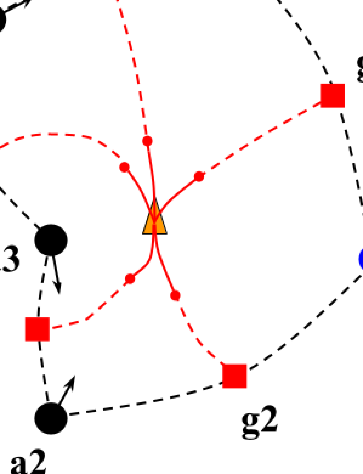
((a)) DAGap synthesizes multiple trajectories (red, dashed lines) based on detected gaps.

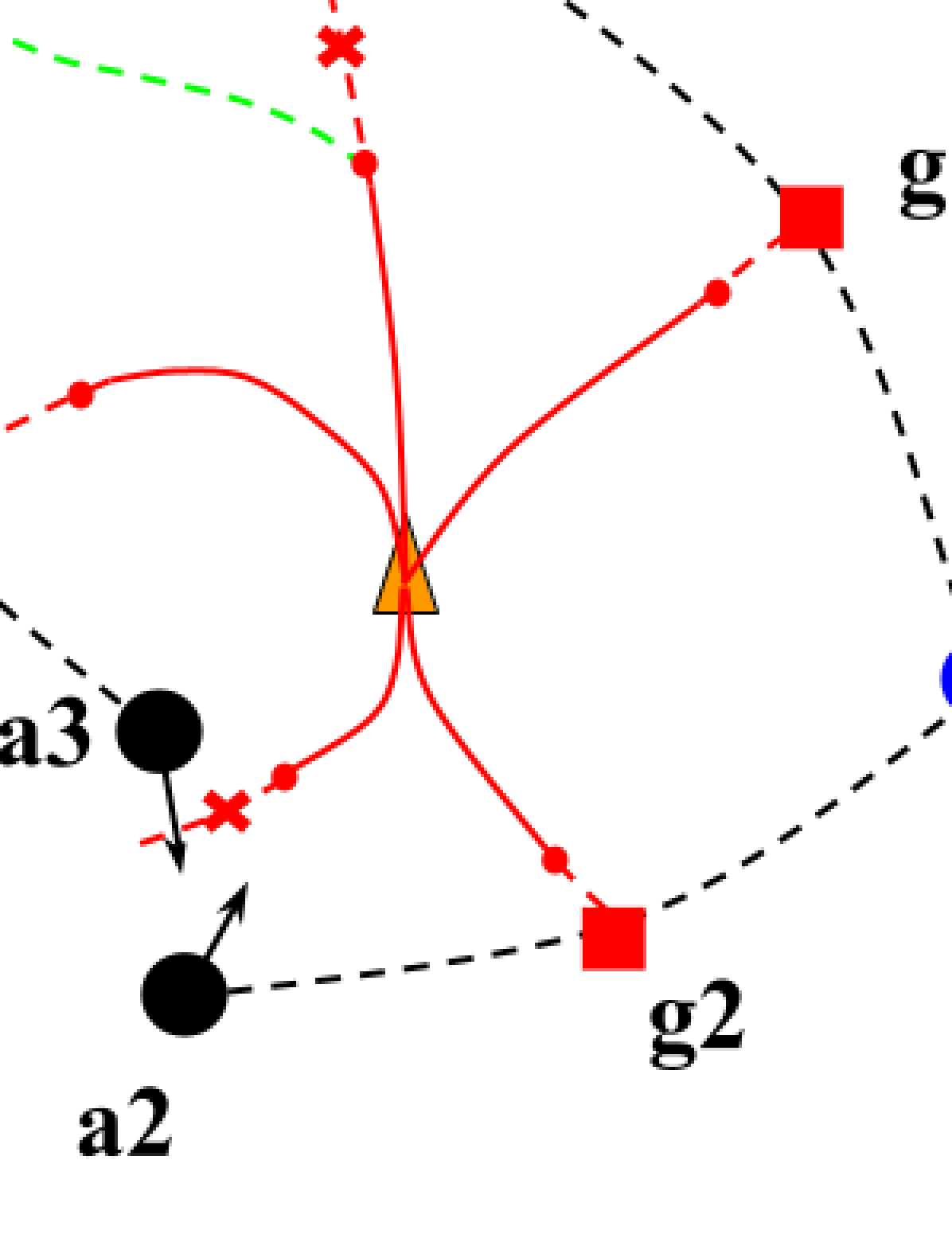
((b)) DAGap trajectory updates for newly-opened (green) and closed gaps (red x).

Figure 3: DAGap synthesizes and updates trajectories.

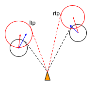
Figure 4: Inflated agent gap detection. Black and red circles are the initial and expanded inflated circles. Red and blue arrows are the estimated and true agent’s velocity. Ltp and rtp mean left and right tangent point, respectively.

Two problems need to be resolved. First, how to synthesize the trajectory to accommodate to the spatio-temporal dynamics of an open gap. For this, we predict the agents’ positions based on the Kalman filter, construct a predicted scan $\mathcal{L}$, and recover predicted gaps and gap regions for $N$ steps into the future. Each gap defines a local gap goal. When all gap goals are connected to the robot, they define a star-like graph. $N$ repeated single-step iterations following the PGap gradient field [5] using the predicted gaps synthesizes a set of candidate trajectories. This reactive approach is computationally fast.

Predicted future gaps states may lead to a new gap or have a previously-open gap close. These birth/death events need to be resolved. If a new gap is detected due to agents moving away from each other, like agent4 and agent5 in fig. 3(b), create a trajectory for this newly-open gap at algorithm 1 line 9-10. From all existing trajectories, pick the one closest to the new gap as the path to expand from. This new trajectory will split from the old trajectory towards the new gap. In fig. 3(b), the green trajectory to gap6 is copied from the trajectory to a previously-open but now closed gap5. The previously-open but now closed gap will be labelled as closed and trajectory updating will be halted. After planning finishes, return all trajectories targeting open gaps.

Algorithm 1 DAGap Trajectory Synthesis

1:$\mathcal{T}_{\text{S}}\leftarrow TrajectorySet$

2:$\mathcal{G}_{\text{S}}\leftarrow GapSet$

3:function DAGap($\mathcal{L}^{inf}$)

4:     for $\texttt{horizon}=1,2,\ldots,N$ do

5:         $\mathcal{G}_{\text{S}}\leftarrow$ gapDection($\mathcal{L}^{inf}$)

6:         if $\texttt{horizon}==1$ then

7:              initialize $\mathcal{T}$ for $G\in\mathcal{G}_{\text{S}}$ and add into $\mathcal{T}_{\text{S}}$

8:         end if

9:         for $G\in\mathcal{G}_{\text{S}}$ do

10:              if $\mathcal{T}$ of $G$ doesn’t exist in $\mathcal{T}_{\text{S}}$ then

11:                  initialize $\mathcal{T}$ for $G$ and add into $\mathcal{T}_{\text{S}}$

12:              end if

13:              $\mathcal{T}$ one step forward towards $G$ using PFM

14:         end for

15:         update the agents’ $\mathcal{L}^{inf}$ with kalman filter

16:     end for

17:return $\mathcal{T}_{\text{S}}$

18:end function

III-B Trajectory optimization and scoring

A set of trajectories $\mathcal{T}_{\text{S}}$ is generated from the algorithm 1. Each trajectory considers the specific pairwise agents forming its gap, which is acceptable in static environments. Dynamic agents can drive towards the robot outside the gap region. It’s risky if the robot doesn’t plan in advance, especially when agents move fast. Thus the second problem is to ensure safety constraint satisfaction for all agents over the planning horizon. The CFS optimizer, which can efficiently find optimal solutions that are strictly safe, is adopted to further modify these reference trajectories $\mathcal{T}_{\text{S}}$. Compared to other optimization methods like sequential quadratic programming (SQP), CFS exploits problem geometry to improve computational efficiency while solving the optimization, which is critical for online planning [9].

For each trajectory, robot with initial pose $\bm{x}_{0}$ at time $t$ is suppose to reach a local goal position $\bm{x}_{lgoal}$ at time $t+T$ . Let $T=N\Delta t$ , where $N$ is the planning horizon and $\Delta t$ is the discrete time interval. The robot trajectory is denoted as $\bm{s}=[\bm{x}^{[0]};...;\bm{x}^{[i]};...;\bm{x}^{[N-1]}]$, where $\bm{x}^{[0]}=\bm{x}_{0}$ , and $\bm{x}^{[N-1]}=\bm{x}_{goal}$. The trajectory of agent $j$ is denoted as $\bm{s}_{O}^{j}=[\bm{o}^{[0]}_{j};...;\bm{o}^{[i]}_{j};...;\bm{o}^{[N-1]}_{j}]$, where $j\in\{1,2,...,M\}$ and $M$ means the number of agents. Therefore, the robot should plan the trajectory that can reach the local goal while keeping the safety distance $r_{\emph{ins}}$ from all agents for every time step. Mathematically, the discretized optimization problem is formulated as:

$$\min_{\bm{s}}\leavevmode\nobreak\ \|\bm{s}-\bm{s}_{r}\|_{Q_{r}}^{2}+\|\bm{s}\|_{Q_{s}}^{2},$$ (1a)

$$s.t.\leavevmode\nobreak\ D(\bm{x}^{[i]},\bm{o}^{[i]}_{j})\geq r_{\emph{ins}},\forall i,\forall j,$$ (1b)

$$\bm{x}^{[1]}=\bm{x}_{0},\bm{x}^{[M]}=\bm{x}_{lgoal}$$ (1c)

where $\|\bm{s}-\bm{s}_{r}\|_{Q_{r}}^{2}$ penalizes the deviation from the new trajectory to the reference trajectory, and $\|\bm{s}\|_{Q_{s}}^{2}$ penalizes the properties of the new trajectory itself which ensures low velocity and acceleration magnitude. Constraint $D(\bm{x}^{[i]},\bm{o}^{[i]}_{j})\geq r_{\emph{ins}}$ requires that the robot should keep safe at each planning step, where $D(.\,,.)$ computes the Euclidean distance between two points. The trajectory scoring eq. 2 combines global target goal efficiency and optimization cost. The trajectory with highest score will be selected to follow:

$$J(\mathcal{T})=D(target,\bm{x}^{[M]})-\|\bm{s}-\bm{s}_{r}\|_{Q_{r}}^{2}-\|\bm{s}\|_{Q_{s}}^{2}\\$$ (2)

III-C Uncertainty Analysis and Replanning

In the above process, the safety distance is a fixed value $r_{\emph{ins}}$ that will work with perfect prediction about agents’ trajectories. In uncertain world, however, estimated agent positions and velocities from the Kalman filter have errors that will propagate as planning horizon increases. Using a fixed safety distance $r_{\emph{ins}}$ may lead to collision. To mitigate this problem, enlarge the safety distance according to the estimated high-confidence bound of prediction errors. Assume the agent has constant velocity. Denote the current estimated agent state as $\bm{z}^{[0]}=\left[\begin{matrix}\bm{o}^{[0]};\bm{v}\end{matrix}\right]$, including position $\bm{o}^{[0]}$ and velocity $\bm{v}$, and its estimated covariance matrix as $\bm{\Sigma_{0}}$. The ground truth state is labeled as $\bm{z^{[0]}}_{*}$. The future agent state predicted at step $i$ is $\bm{z}^{[i]}=F^{i}\bm{z}^{[0]}$, where $F$ represents the transfer matrix. Suppose $\bm{z}^{[0]}\sim\mathcal{N}(\bm{z}^{[0]}_{*},\,\bm{\Sigma}_{0})$, the prediction for $\bm{z}^{[i]}$ should follow the distribution: $\bm{z}^{[i]}\sim\mathcal{N}(\bm{z}^{[i]}_{*},\,\bm{\Sigma_{i}})$, where $\bm{\Sigma_{i}}$ is the covariance matrix propagated forward for $i$ steps $\bm{\Sigma_{i}}=(F^{T})^{i}\bm{\Sigma_{0}}F^{i}$. Pick out the submatrix of $\bm{\Sigma_{i}}$ corresponding to the position $\bm{o}^{[i]}$ and denote the position covariance matrix as $\bm{\Sigma_{i,o}}$. Then the error $\Delta\bm{o}^{[i]}=\bm{o}^{[0]}-\bm{o}^{[0]}_{*}$ should follow the chi-square distribution ${\chi}^{2}_{N}$ as eq. 3, where $N$ is the dimension of $\bm{o^{[i]}}$,

$$(\bm{\Delta o^{[i]})}^{T}\,\bm{\Sigma_{i,o}}^{-1}\,\bm{\Delta o^{[i]}}\sim{\chi}^{2}_{N}$$ (3)

with the probability support on confidence bound value $k_{\epsilon}$:

$$P((\bm{\Delta o^{[i]})}^{T}\,\bm{\Sigma_{i,o}}^{-1}\,\bm{\Delta o^{[i]}}\leq k_{\epsilon})>1-\epsilon$$ (4)

based on Lemma 4 in [38]. The following bound on the error $\bm{\Delta o^{[i]}}$ holds with probability $1-\epsilon$:

$$-\sqrt{k_{\epsilon}\lambda_{n}}\leq\bm{v_{n}}^{T}\bm{\Delta o^{[i]}}\leq\sqrt{k_{\epsilon}\lambda_{n}},\forall n\\$$ (5)

where $\{\lambda_{n}\}’s$ and $\{\bm{v_{n}}\}’s$ are the eigenvalues and eigenvectors of $\bm{\Sigma_{i,o}}$, $n\in\{1,2,...,N\}$. Since the $\{\bm{v_{n}}\}’s$ are perpendicular bases, $\bm{\Delta o^{[i]}}$ can be represented as $\sum_{n}a_{n}\bm{v_{n}}$, where $a_{n}$ is the coefficient,

$$\bm{v_{n}}^{T}\bm{\Delta o^{[i]}}=\bm{v_{n}}^{T}\sum_{k}a_{k}\bm{v_{k}}=a_{n}\|\bm{v_{n}}\|$$ (6a)

$$-\frac{\sqrt{k_{\epsilon}\lambda_{n}}}{\|\bm{v_{n}}\|}\leq a_{n}\leq\frac{\sqrt{k_{\epsilon}\lambda_{n}}}{\|\bm{v_{n}}\|}$$ (6b)

$$\|\bm{\Delta o^{[i]}}\|=\|\sum_{n}a_{n}\bm{v_{n}}\|\leq\sum_{n}\sqrt{k_{\epsilon}\lambda_{n}}$$ (6c)

Theorem 1

Using the bounds in eq. 6c, increasing the safety distance by $\sum_{n}\sqrt{k_{\epsilon}\lambda_{n}}$ guarantees safety with probability at least $1-\epsilon$.

Proof:

Since the prediction of the ground truth agent’s position $\bm{o}^{[i]}_{*}$ is unbounded, we ensure a probability safety constraint between $\bm{x}^{[i]}$ and $\bm{o}^{[i]}_{*}$ for $\forall i$,

$$P(\|\bm{x}^{[i]}-\bm{o}^{[i]}_{*}\|\geq r_{\emph{ins}})<1-\epsilon$$ (7)

At worst case, $\|\bm{x}^{[i]}-\bm{o}^{[i]}_{*}\|=\|\bm{x}^{[i]}-\bm{o}^{[i]}+\bm{o}^{[i]}-\bm{o}^{[i]}_{*}\|=|\|\bm{x}^{[i]}-\bm{o}^{[i]}\|-\|\bm{o}^{[i]}-\bm{o}^{[i]}_{*}\||$. From eq. 6c, the bound on the uncertainty $\|\bm{o}^{[i]}-\bm{o}^{[i]}_{*}\|$ holds with probability $1-\epsilon$. Expanding the safety distance $d_{safe}$ between the robot and the estimated agent position $\|\bm{x}^{[i]}-\bm{o}^{[i]}\|$ to $r_{\emph{ins}}+r$, where $r=\sum_{n}\sqrt{k_{\epsilon}\lambda_{n}}$, guarantees safety with probability at least $1-\epsilon$. ∎

Based theorem 1, estimate the robust safety distance $d_{safe}=r_{\emph{ins}}+r$ for every agent and replace the fixed $r_{\emph{ins}}$ used in DAGap and CFS (see fig. 2). As a detection threshold, larger values of $d_{safe}$ increase the likelihood of false negatives (e.g., rejection of passable paths), which limits the planning space and leads to more conservative behavior. To avoid this problem, we set an upper bound of the $d_{safe}$ and record the first time step $k$ this upper bound is reached. Replanning is evoked after executing $k$ steps due to low safety likelihood, see algorithm 2 line 18.

Algorithm 2 H-DAGap Algorithm

1:$\mathcal{U}_{\text{a}}\leftarrow uncertaintyAnalyzor$

2:$\mathcal{D}_{\text{s}}\leftarrow$ robust safe distances $d_{safe}^{i}$, $i\in\{1,2...N\}$

3:$\texttt{k}\leftarrow$ replan step

4:function Traj Optimization($\mathcal{T}_{\text{S}}$, $\mathcal{U}_{\text{a}}$)

5:     for $\mathcal{T}\in\mathcal{T}_{\text{S}}$ do

6:         compute $\mathcal{D}_{\text{s}},\texttt{k}$ with $\mathcal{U}_{\text{a}}$

7:         CFS optimizes and scores $\mathcal{T}$ using $\mathcal{D}_{\text{s}}$

8:     end for

9:     return $\mathcal{T}$ with highest score and its k

10:end function

11:

12:while not arrive goal area do

13:     $\mathcal{T}_{\text{S}}$ $\leftarrow$ DAGap($\mathcal{L}^{inf}$)

14:     $\mathcal{T},\texttt{k}$ $\leftarrow$ Traj Optimization($\mathcal{T}_{\text{S}}$, $\mathcal{U}_{\text{a}}$)

15:     stepCount = 0

16:     for next waypoint p in $\mathcal{T}$ do

17:         safe control u $\leftarrow$ SSA(p)

18:         execute u and $\texttt{stepCount}\mathrel{+}=1$

19:         break for replan if $\texttt{stepCount}\geq\texttt{k}$

20:     end for

21:end while

III-D Safe Controller

Even though DAGap and CFS are efficient planning methods, their longer horizon mean that they are more computationally expensive compared to one-step reactive safe control methods. Moreover, challenging crowded environments mean that CFS may not have converged within a few iterations. Due to the real-time planning requirement, we don’t run CFS for all synthesized trajectories until they converge. Instead we select the top two trajectories based on the efficiency score $D(target,\bm{x}^{[M]})$ as we notice the optimization cost doesn’t change the rank ordering of top two candidates in most cases, and run CFS for only one iteration. Moreover, we adopt fast SSA in the low-level controller layer to further compensate the long planning time, and monitor the control at every step. Compared to other reactive algorithms like CBF which enforces constraints everywhere, SSA achieves better safety-efficiency trade-off in complex environment [13].

The key of SSA is to define a valid safety index $\phi$ such that 1) there always exists a feasible control input in control space that satisfies $\dot{\phi}\leq-\eta\phi$ when $\phi\geq 0$ and 2) any control sequences that satisfy $\dot{\phi}\leq-\eta\phi$ when $\phi\geq 0$ ensures forward invariance and asymptotic convergence to the safe set $X_{S}$, $\eta$ is a positive constant that adjusts the convergence rate. In our problem, $X_{S}=\left\{x|\phi_{0}(x)\leq 0\right\}$, where $\phi_{0}$ is defined as $d_{min}^{2}-d^{2}$, $d_{min}$ is the user defined minimal distance and $d$ is the distance from the robot to the agent. Since the robot we adopt in testing is a second-order system, we add higher order term of $\phi_{0}$ to ensure that relative degree one from safety index $\phi$ to the control input, and $\phi$ is defined as follows:

$$\phi=d_{min}^{2}-d^{2}-k\cdot\dot{d}.$$ (8)

where $\dot{d}$ is the relative velocity from the robot to the agent and $k$ is a constant factor. As proved in [12][39], the safety index $\phi$ will ensure forward invariance of the set $\phi\leq 0\cap\phi_{0}\leq 0$ and global attraction to that set. With safety index $\phi$, project the reference control $u^{r}$ to the set of safe controls that satisfy $\dot{\phi}\leq-\eta\,\phi$ when $\phi\geq 0$, and $\dot{\phi}$ is expressed as

$$\dot{\phi}=\frac{\partial\phi}{\partial x}\,f+\frac{\partial\phi}{\partial x}\,g\;u=L_{f}\phi+L_{g}\phi\;u.$$ (9)

Compute $\phi_{j}$ for every agent and add the safety constraint whenever $\phi_{j}$ is positive. SSA solves the following one-step optimization problem, with safety and dynamics constraints, through quadratic programming (QP) when triggered:

$$\underset{u\in U}{\min}\, ||u-u^{r}||^{2}=\underset{u\in U}{\min}\,u^{\mathrm{T}}\left[\begin{matrix}1&0\\ 0&1\end{matrix}\right]u-2u^{\mathrm{T}}\left[\begin{matrix}1&0\\ 0&1\end{matrix}\right]u^{r}$$ (10a)

$$s.t.L_{f}\phi_{j}+L_{g}\phi_{j}\leavevmode\nobreak\ u\leq-\eta\,\phi_{j},j\in\{1,2...M\}.$$ (10b)

IV Experiments

This section covers the experiments, results, and comparison of H-DAGap with ARENA [17] and DRRT-ProbLP [18].

IV-A Benchmark Results

Experiments are conducted in a $2\times 2$ empty world, see fig. 5, with 20 and 50 dynamic agents in two test scenarios. ARENA nd DRRT-ProbLP are tested in 20 agents environments [17][18], and we test our model in the same condition for comparison and also increase the agents’ number to 50 to test their capability in more challenging scenario. The radius of agents is 0.05 and the velocity is sampled from a uniform distribution $\left[5e^{-3},2e^{-2}\right]$. Agents can move randomly in any direction in the map and collisions between them are not considered. The robot adopts the second order unicycle model and with speed range $\left[0,2e^{-2}\right]$. The overall scenario settings used in ours and two baseline papers are similar, including the relatively agent size to world size and the relatively agent velocity to robot velocity. But we don’t assume the perfect lidar measurement is available, instead, the 360^∘ field of view (FoV) measurement has errors following the Gaussian distribution $\mathcal{N}(0,\,0.01^{2})$. We use Kalman filter to track the position and velocity of each agent inside the $0.2$ sensing range. Compare to the environment used in previous safe learning work [13], we enlarge the agent size, increase its top speed, and add measurement uncertainty, which makes the task more challenging. H-DAGap is run in Python on Ubuntu 20.04 of 3.7 GHz using Intel Core i7. The average computate times for DAGap, CFS and SSA are $0.0814s$, $0.1120s$ and $6.854\mathrm{e}{-4}s$ respectively. We conduct 100 test runs in each scenario and use collision rate and success rate as evaluation metrics. A success trial means the robot reaches the goal within 3500 steps without any collision. The robot is allowed to continue driving after collision in benchmark papers. We follow this rule but don’t observe multiple collisions in any H-DAGap trial.

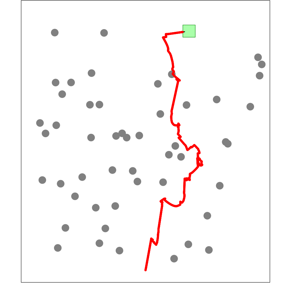
Figure 5: Testing environment with 50 dynamic agents. The green square is the target goal, the gray circles are agents’ positions at last time step and the red path is the entire robot trajectory from the start to the goal.

ARENA and DRRT-ProbLP are used for safe navigation in crowded dynamic environments and tested in environment with 20 dynamic agents in their papers. H-DAGap achieves $97\%$ success rate and only $3\%$ collision rate in the 50 dynamic agents environment (see table I), which bests the benchmark implementations in the 20 agent environment. For DRRT-ProbLP planner, the DRRT module only considers static obstacles and the avoidance of dynamic agents is entirely handled by ProbLP. ProbLP samples the robot movement direction based on the distribution of target goal and agents, then synthesizes and scores the trajectories. However, there are usually many safe trajectories in open continuous space; Sampling-based methods can’t enumerate all of them and inevitably become suboptimal. ARENA combines the traditional global planner A* and the Deep Reinforcement Learning based (DRL) local planner. Vanilla A* doesn’t consider the dynamic agent and DRL doesn’t consistently ensure safety constraint satisfaction during execution. On the other hand, H-DAGap considers and probabilistically guarantees safety in both layers and in multi-modules.

Table I: H-DAGap and benchmark algorithms outcomes in an empty world with 20 and 50 dynamic agents.

	20 agents		50 agents
Model	Success	Collision	Success	Collision
H-DAGap	100%	0%	97%	3%
DRRT-ProbLP	N/A	4%	N/A	N/A
ARENA	$\leq$ 92.7%	23.7%	N/A	N/A

IV-B Discussion

This section looks into the contribution of different modules. Each experiment is repeated 100 times. Here, the test run will stop once the robot collides.

DAGap trajectory synthesis result: We compare the results of DAGap only and static gap detection (SGap), which synthesize trajectories for the gaps detected at current time step. CFS optimization and SSA modification are not applied. Compared to SGap, DAGap reduces the collision rate by $13\%$ and $7\%$ in 20 and 50 agent environments respectively, see table II. The reason is that DAGap considers the spatio-temporal dynamics of open gaps and filters out the trajectories towards gradually closing gaps. SGap guarantees safe passage in static environments, however, the originally open gap may become closed and can lead to collision in dynamic environments. The improvement of incorporating spatio-temporally evolving information is greater for the easy scenario because DAGap is less affected by the agents outside the gap region due to the lower agents density.

Table II: Experimental results of each module.

	20 agents		50 agents
Model	Collision	Success	Collision	Success
SGap	49%	51%	76%	24%
DAGap	36%	64%	69%	31%
DAGap+CFS	8%	92%	29%	71%
DAGap+CFS+SSA	0%	100%	3%	97%

CFS trajectory optimization result: The collision rate drops from $69\%$ to $29\%$ in the 50 agent scenario after CFS optimization and uncertainty-based safety distance adjustment. Compared to using CFS directly, DAGap provides good initial trajectories that can improve the safety of optimized trajectories. To better explain it, we need to define the feasibility of a trajectory: a feasible trajectory requires the distances between all neighbouring waypoints be smaller than a threshold value related to the robot’s maximal velocity. An infeasible trajectory increases the risk of collision and is hard to be tracked by robot due to the large jump between waypoints. The feasibility rate of CFS optimized trajectory is around $87.4\%$ when using DAGap to generate initial reference trajectory that drives towards the affordance free space, but is only $66.9\%$ without DAGap.

SSA safe controller result: By replacing the feedback controller with the SSA safe controller, the collision rate drops to $3\%$. There are two main reasons behind: first of all, as we discussed above, CFS may generate dynamically infeasible trajectory due to the limited number of optimization iterations we can run in real-time and the challenging crowded dynamic environment. Tracking infeasible trajectory can cause collision. SSA modifies these unreasonable tracking controls online. Secondly, DAGap and CFS are long-term planners considering N steps safety. But the predicted error of trajectories of agents will compound as time goes, making the planned trajectory risky in the long-term future even we expand the safety distance. On the other hand, because of its fast computation property, SSA always uses the latest information to calculate the one-step safe control and to reduce collision caused by uncertainty.

Collision analysis: Even applying all these techniques, there is still a $3\%$ collision rate. The collisions are categorized into two main cases: multi-agent traps and a fast, overtaking agent. Notice, the agents in our environments are artificial and the collisions between agents are allowed. In the first case, trapping occurs when a gap detected as passable is actually not passable (i.e., a false positive) or when an existing or future gap is not detected due to sensing radius limits. The robot ends up trapped by multiple converging agents, see fig. 6(a), and SSA cannot find a control to meet all safety constraints because the robot will get closer to one of the agents no matter in which direction it drives. The “best” control for SSA is to stay put. The second case happens when a fast agent driving behind the robot and in collision overtakes it. Following the safest one-step control generated by SSA, moves the robot in a direction aligning with the agent’s velocity even if the DAGap trajectory points in another direction. Alignment occurs because SSA modifies the original control to the safest single-step one based on the safety index. This escape-and-pursue situation usually continues for several steps until the robot meets another agent and needs to take a new control to avoid both. The fast agent behind will then catch up such that the robot cannot bypass both within one or two steps due to its size and speed. From the perspective of SSA, no control exists to satisfy the constraints in eq. 10b once the new agent enters the sensing radius. The situations can be avoided through high-level modifications. One high-level planner design change would be to check if there may be future trapping situations, then specify an alternative detouring (global) goal until the danger is resolved. Additionally better coordination between the high-level planner layer and low-level SSA layer can avoid conflicts related to the safety specifications. We leave these to future improvements.

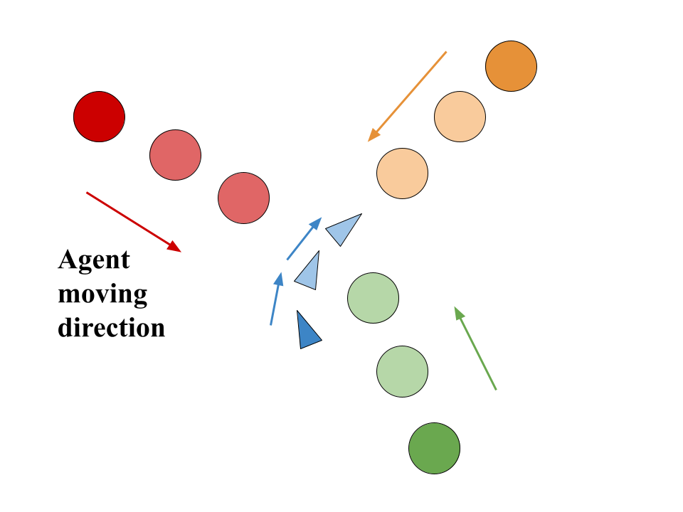
((a)) Trapping collision

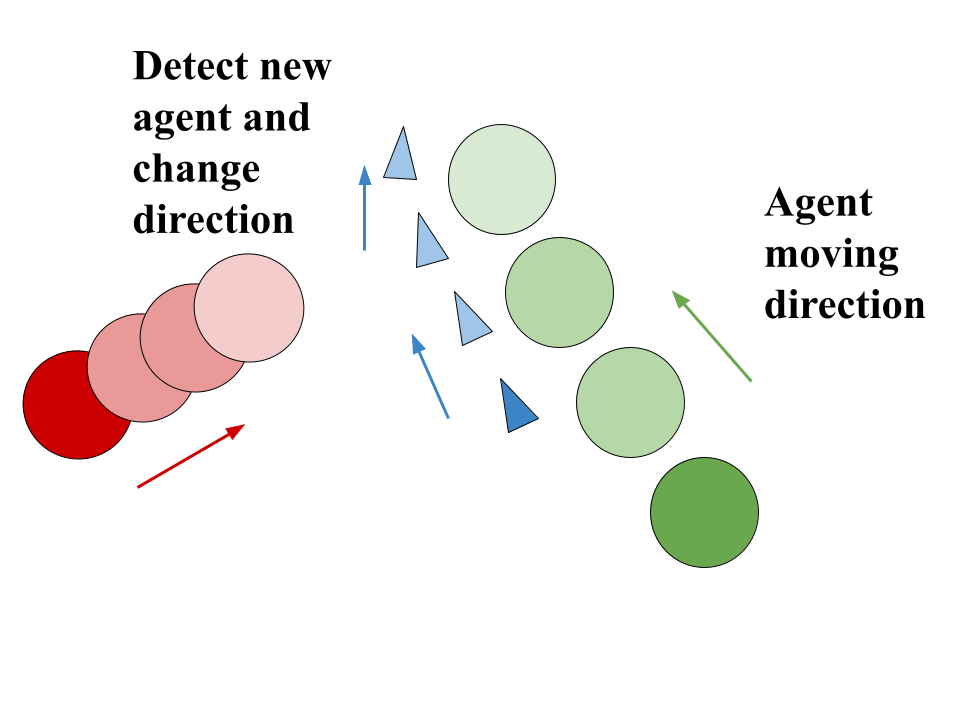
((b)) Overtaking collision

Figure 6: Trapping collision and overtaking collision. The robot is the blue triangle and the agents are colored circles. All are a darker hue at their initial positions and lighten as time progresses.

V Conclusion

This work described and evaluated H-DAGap, a hierarchical navigation solution containing a multi-phase planner and a low-level safe controller. It is a solution strategy to the safe navigation problem in crowded, dynamic and uncertain environments. Estimated high-confidence error bounds are used in the planner to achieve provably high probability safety to uncertainty. Conducted experimental benchmarking in simulation and analysis confirm the effectiveness of H-DAGap at avoiding collisions and navigating to the goal. The H-DAGap implementation is available at https://github.com/hychen-naza/H-DAGap. Improved coordination between the high-level planning and low-level safety control to improve collisions in low-probability robot-agent configurations is left to future work. Extension of H-DAGap to consider the case of reduced field of view sensing is also left to future work.

References

- [1] M. Hoy, A. S. Matveev, and A. V. Savkin, “Algorithms for collision-free navigation of mobile robots in complex cluttered environments: a survey,” Robotica, p. 463–497, 2015.
- [2] F. Bonin-Font, A. Ortiz, and G. Oliver, “Visual navigation for mobile robots: a survey,” Journal of Intelligent and Robotic Systems, pp. 263–296, 2008.
- [3] D. Zhu and J.-C. Latombe, “New heuristic algorithms for efficient hierarchical path planning,” IEEE Transactions on Robotics and Automation, pp. 9–20, 1991.
- [4] J. Guldner, V. Utkin, and R. Bauer, “Mobile robots in complex environments: a three-layered hierarchical path control system,” in IEEE International Conference on Intelligent Robots and Systems, 1994, pp. 1891–1898.
- [5] R. Xu, S. Feng, and P. A. Vela, “Potential gap: a gap-informed reactive policy for safe hierarchical navigation,” IEEE Robotics and Automation Letters, pp. 8325–8332, 2021.
- [6] M. Mujahad, D. Fischer, B. Mertsching, and H. Jaddu, “Closest gap based (cg) reactive obstacle avoidance navigation for highly cluttered environments,” in IEEE/RSJ International Conference on Intelligent Robots and Systems, 2010, pp. 1805–1812.
- [7] M. Demir and V. Sezer, “Improved follow the gap method for obstacle avoidance,” in IEEE International Conference on Advanced Intelligent Mechatronics, 2017, pp. 1435–1440.
- [8] J. S. Smith, R. Xu, and P. Vela, “egoteb: Egocentric, perception space navigation using timed-elastic-bands,” in IEEE International Conference on Robotics and Automation, 2020, pp. 2703–2709.
- [9] C. Liu, C.-Y. Lin, Y. Wang, and M. Tomizuka, “Convex feasible set algorithm for constrained trajectory smoothing,” in American Control Conference, 2017, pp. 4177–4182.
- [10] O. Khatib, “Real-time obstacle avoidance for manipulators and mobile robots,” in IEEE International Conference on Robotics and Automation, 1985, pp. 500–505.
- [11] A. D. Ames, J. W. Grizzle, and P. Tabuada, “Control barrier function based quadratic programs with application to adaptive cruise control,” in IEEE Conference on Decision and Control, 2014, pp. 6271–6278.
- [12] C. Liu and M. Tomizuka, “Control in a safe set: Addressing safety in human-robot interactions,” in Dynamic Systems and Control Conference, 2014.
- [13] H. Chen and C. Liu, “Safe and sample-efficient reinforcement learning for clustered dynamic environments,” IEEE Control Systems Letters, pp. 1928–1933, 2022.
- [14] M. A. Kareem Jaradat, M. Al-Rousan, and L. Quadan, “Reinforcement based mobile robot navigation in dynamic environment,” Robotics and Computer-Integrated Manufacturing, pp. 135–149, 2011.
- [15] L. Liu, D. Dugas, G. Cesari, R. Siegwart, and R. Dubé, “Robot navigation in crowded environments using deep reinforcement learning,” in IEEE/RSJ International Conference on Intelligent Robots and Systems, 2020, pp. 5671–5677.
- [16] K. Li, Y. Lu, and M. Q.-H. Meng, “Human-aware robot navigation via reinforcement learning with hindsight experience replay and curriculum learning,” in IEEE International Conference on Robotics and Biomimetics, 2021, pp. 346–351.
- [17] L. Kästner, T. Buiyan, X. Zhao, L. Jiao, Z. Shen, and J. Lambrecht, “Arena-rosnav: Towards deployment of deep-reinforcement-learning-based obstacle avoidance into conventional autonomous navigation systems,” IEEE/RSJ International Conference on Intelligent Robots and Systems, pp. 6456–6463, 2021.
- [18] M. D’Arcy, P. Fazli, and D. Simon, “Safe navigation in dynamic, unknown, continuous, and cluttered environments,” in IEEE International Symposium on Safety, Security and Rescue Robotics, 2017, pp. 238–244.
- [19] A. Stentz, “The focussed d* algorithm for real-time replanning,” in International Joint Conference on Artificial Intelligence, 1995, p. 1652–1659.
- [20] M. Likhachev and D. Ferguson, “Planning long dynamically feasible maneuvers for autonomous vehicles,” The International Journal of Robotics Research, pp. 933–945, 2009.
- [21] M. Zucker, J. Kuffner, and M. Branicky, “Multipartite rrts for rapid replanning in dynamic environments,” in IEEE International Conference on Robotics and Automation, 2007, pp. 1603–1609.
- [22] M. Phillips and M. Likhachev, “Sipp: Safe interval path planning for dynamic environments,” in IEEE International Conference on Robotics and Automation, 2011, pp. 5628–5635.
- [23] S. Petti and T. Fraichard, “Safe motion planning in dynamic environments,” in IEEE/RSJ International Conference on Intelligent Robots and Systems, 2005, pp. 2210–2215.
- [24] M. Branicky, M. Curtiss, J. Levine, and S. Morgan, “Sampling-based planning, control and verification of hybrid systems,” Control Theory and Applications, IEE Proceedings -, pp. 575– 590, 2006.
- [25] D. Hsu, R. Kindel, J.-C. Latombe, and S. Rock, “Randomized kinodynamic motion planning with moving obstacles,” The International Journal of Robotics Research, pp. 233–255, 2002.
- [26] C. Park, J. Pan, and D. Manocha, “Itomp: Incremental trajectory optimization for real-time replanning in dynamic environments,” in International Conference on Automated Planning and Scheduling, 2012, pp. 207–215.
- [27] W. Xu, J. Wei, J. M. Dolan, H. Zhao, and H. Zha, “A real-time motion planner with trajectory optimization for autonomous vehicles,” in IEEE International Conference on Robotics and Automation, 2012, pp. 2061–2067.
- [28] J. Yu and S. M. LaValle, “Optimal multirobot path planning on graphs: complete algorithms and effective heuristics,” IEEE Transactions on Robotics, pp. 1163–1177, 2016.
- [29] A. Agrawal and K. Sreenath, “Discrete control barrier functions for safety-critical control of discrete systems with application to bipedal robot navigation.” in Robotics: Science and Systems, 2017.
- [30] L. Gracia, F. Garelli, and A. Sala, “Reactive sliding-mode algorithm for collision avoidance in robotic systems,” IEEE Transactions on Control Systems Technology, pp. 2391–2399, 2013.
- [31] G. Li, A. Yamashita, H. Asama, and Y. Tamura, “An efficient improved artificial potential field based regression search method for robot path planning,” in IEEE International Conference on Mechatronics and Automation, 2012, pp. 1227–1232.
- [32] J. Guldner and V. Utkin, “Sliding mode control for gradient tracking and robot navigation using artificial potential fields,” IEEE Transactions on Robotics and Automation, pp. 247–254, 1995.
- [33] J. v. d. Berg, S. J. Guy, M. Lin, and D. Manocha, “Reciprocal n-body collision avoidance,” in Robotics research. Springer, 2011, pp. 3–19.
- [34] J. Van den Berg, M. Lin, and D. Manocha, “Reciprocal velocity obstacles for real-time multi-agent navigation,” in IEEE International Conference on Robotics and Automation, 2008, pp. 1928–1935.
- [35] R. Cheng, G. Orosz, R. Murray, and J. Burdick, “End-to-end safe reinforcement learning through barrier functions for safety-critical continuous control tasks,” in Proceedings of AAAI Conference on Artificial Intelligence, 2019, pp. 3387–3395.
- [36] J. S. Smith, S. Feng, F. Lyu, and P. A. Vela, Real-time egocentric navigation using 3D sensing, 2020, pp. 431–484.
- [37] C. Roesmann, W. Feiten, T. Woesch, F. Hoffmann, and T. Bertram, “Trajectory modification considering dynamic constraints of autonomous robots,” in German Conference on Robotics, 2012, pp. 1–6.
- [38] R. Cheng, M. J. Khojasteh, A. D. Ames, and J. W. Burdick, “Safe multi-agent interaction through robust control barrier functions with learned uncertainties,” in IEEE Conference on Decision and Control, 2020, pp. 777–783.
- [39] W. Zhao, T. He, and C. Liu, “Model-free safe control for zero-violation reinforcement learning,” in Proceedings of the Conference on Robot Learning, 2021, pp. 784–793.