TIC 219006972: A Compact, Coplanar Quadruple Star System Consisting of Two Eclipsing Binaries with an Outer Period of 168 days

Abstract

We present the discovery of a new highly compact quadruple star system, TIC 219006972, consisting of two eclipsing binary stars with orbital periods of 8.3 days and 13.7 days, and an outer orbital period of only 168 days. This period is a full factor of 2 shorter than the quadruple with the shortest outer period reported previously, VW LMi, where the two binary components orbit each other every 355 days. The target was observed by TESS in Full-Frame Images in sectors 14-16, 21-23, 41, 48 and 49, and produced two sets of primary and secondary eclipses. These show strongly non-linear eclipse timing variations (ETVs) with an amplitude of $\sim$0.1 days, where the ETVs of the primary and secondary eclipses, and of the two binaries are all largely positively correlated. This highlights the strong dynamical interactions between the two binaries and confirms the compact quadruple configuration of TIC 219006972. The two eclipsing binaries are nearly circular whereas the quadruple system has an outer eccentricity of about 0.25. The entire system is nearly edge-on, with a mutual orbital inclination between the two eclipsing binary star systems of about 1 degree.

1 Introduction

Gravitationally-bound systems of two or more stars are a natural product of star formation and serve as important tracers of the processes and mechanisms driving stellar evolution. When the constituent stars are close enough to each other, the system can experience important (and sometimes quite dramatic) physical and dynamical interactions such as tidal distortions, heating and/or reflection effects, mass transfer, orbital oscillations and/or perturbations, common-envelope events, collisions and even supernovae explosions (e.g. Lidov, 1962; Kozai, 1962; Pejcha et al., 2013; Perets & Fabrycky, 2009; Hamers et al., 2021; Naoz & Fabrycky, 2014; Fang et al., 2018; Fragione & Kocsis, 2019; Liu & Lai, 2019; Borkovits, 2022).

Multiple stellar systems cover a vast range of occurrence rates, orbital configurations, physical parameters, number of components, ages, etc. Overall, about one in every ten Sun-like stars resides in a triple system and a few percent are members of quadruple or higher-order systems (e.g Raghavan et al., 2010; De Rosa et al., 2014; Toonen et al., 2016; Moe & Di Stefano, 2017; Tokovinin, 2017).

Compact multiple star systems are of particular interest for studying dynamical relationships. For example, the current record holders for the confirmed shortest outer periods in triple and quadruple systems are: (i) the 2+1 triple system $\lambda$ Tau with $P_{out}=33.03$ days (Schlesinger, 1916; Ebbighausen & Struve, 1956); (ii) the 2+1+1 quadruple system TIC 114936199 with $P_{middle}\sim 51$ days (Powell et al., 2022a); and (iii) the 2+2 quadruple system VW LMi where the two binary components orbit each other every 355 days (Pribulla et al., 2008, 2020). The outer period of TIC 219006972 is about half as long as that of VW LMi, making it the most compact 2+2 quadruple system reported to date.

Stellar multiples that contain one or more eclipsing binary stars, and have an outer period short enough for detectable interactions between the component sub-systems provide excellent “hunting grounds” for discovery and detailed characterization of triple and higher-order systems. Large-scale photometric surveys are well-positioned to observe such compact multi-stellar systems. For example, NASA’s Transiting Exoplanet Survey Satellite (TESS) mission (Ricker et al., 2015) is expected to observe hundreds of thousands of eclipsing binary stars (Sullivan et al., 2015) and provide high-precision, nearly-continuous month-long observations spanning multiple epochs. Indeed, TESS already demonstrated its potential for stellar multiples by enabling the discovery of hundreds of triple and quadruple systems (e.g. Rappaport et al., 2022; Borkovits et al., 2022; Zasche et al., 2022; Kostov et al., 2022), and even the first two fully eclipsing sextuple systems (Powell et al., 2021; Zasche et al., 2023).

Here we present the latest addition to the still-small family of compact quadruple systems, TIC 219006972, composed of two eclipsing binaries. At the time of writing, TIC 219006972 has the shortest outer orbital period reported, and is the second closest to co-planarity (after TIC 454140642). This paper is organized as follows. Section 2 describes the detection and preliminary analysis of the system. In Section 3, we outline the comprehensive photometric-dynamical solution of the system, followed by a discussion of its properties in Section 4. Section 5 summarizes our results.

2 Detection

TIC 219006972 is a relatively faint (V = 14.312 mag) star in the Northern hemisphere (RA = 14:44:48.71, Dec = +66:22:43.17) with a Gaia DR3 parallax of 6.65 mas/yr, effective temperature of 5651 K, zero $astrometric\_excess\_noise$, and RUWE = 1.01 (Gaia Collaboration et al., 2021). The target is relatively isolated – the closest field star is TIC 1102519834, 17.8 arcsec away and $\Delta$G = 6.2 mag fainter (see Fig. 1), with another 6 sources within 1 arcmin radial search, all $\Delta$G = 4.5 mag and fainter. The parameters of the system are listed in Table 1.

Table 1: Stellar parameters for TIC 219006972

Parameter	Value	Error	Source
Identifying Information
TIC ID	219006972		1
Gaia ID	1669481894221366912		2
$\alpha$ (J2000, hh:mm:ss)	14:44:48.71		1
$\delta$ (J2000, dd:mm:ss)	+66:22:43.17		1
$\mu_{\alpha}$ (mas yr-1)	$6.6476$	0.0174	2
$\mu_{\delta}$ (mas yr-1)	$-3.4518$	0.01511	2
$\varpi$ (mas)	0.7313	0.0133	2
Distance (pc)	1367	32	2
RUWE	1.0121		2
Photometric Properties
$T$ (mag)	13.7021	0.0063	1
$B$ (mag)	14.9	0.106	1
$V$ (mag)	14.312	0.172	1
$Gaia$ (mag)	14.1153	0.0028	2
$J$ (mag)	13.073	0.025	3
$H$ (mag)	12.75	0.025	3
$K$ (mag)	12.676	0.025	3
$W1$ (mag)	12.686	0.022	4
$W2$ (mag)	12.705	0.023	4
$W3$ (mag)	12.582	0.292	4
$W4$ (mag)	9.56		4
Stellar Properties
Teff, Aa (K)	6162	90	This work
Teff, Ab (K)	5942	80	This work
Teff, Ba (K)	5676	110	This work
Teff, Bb (K)	3698	47	This work
$[$Fe/H$]$	-0.275	0.076	This work
Age (Gyr)	6	1.5	This work

Sources: (1) TIC-8 (Stassun et al., 2018), (2) Gaia DR3 (Gaia Collaboration et al., 2021), (3) 2MASS All-Sky Catalog of Point Sources (Skrutskie et al., 2006), (4) AllWISE catalog (Cutri et al., 2012)

TESS observed TIC 219006972 in sectors 14, 15, 16, 21, 22, 23, 41, 48, and 49. The long-cadence TESS photometry for Sectors 48 and 49 is shown in Figure 2, highlighting the two sets of eclipses from binary A (period = 13.7 days) and binary B (period = 8.3 days). We note that there are no clear signatures of stellar rotation in the long-cadence lightcurves.

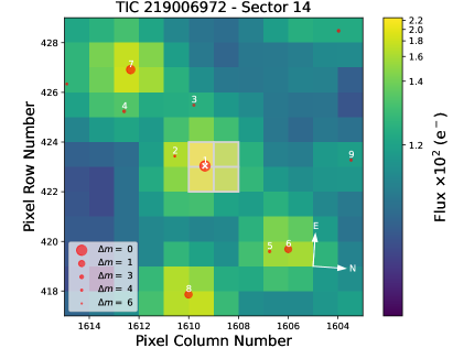
Figure 1: $12\times 12$ TESS pixels image of TIC 219006972 (marked with a cross-hair) for Sector 14 showing all nearby stars brighter than a TESS magnitude difference ${\Delta m=6\ \rm mag}$. Image created with tpfplotter (Aller et al., 2020).

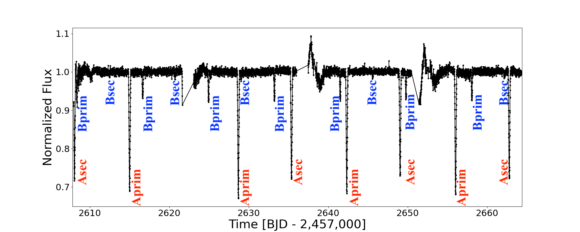
Figure 2: TESS Full-Frame-Image (FFI) eleanor Corrected Flux photometry from Sectors 48 and 49, highlighting select primary and secondary eclipses for both binaries.

TIC 219006972 was initially identified as a target of interest through visual survey of a data set of lightcurves with a high probability of containing eclipses generated from the TESS sector 48 data release. Briefly, upon the release of the Full Frame Images (FFI) from each TESS sector, we download the FFI data and construct all lightcurves brighter than 15 magnitude using the Discover supercomputer at the NASA Center for Climate Simulation. We then process the lightcurves through a neural network trained to identify eclipses, further described in Powell et al. (2022b). We selected the lightcurves identified by the neural network as likely containing eclipses, and distributed them to the Visual Survey Group (VSG, Kristiansen et al., 2022) for visual review.

Using the LcTools software system (Schmitt et al., 2019; Schmitt & Vanderburg, 2021), members of the VSG identified TIC 219006972 as a likely multiple star system in December 2022 with periods of PA = 13.7 days and PB = 8.3 days (upper panels, Fig. 3), and the target was accordingly promoted for additional analysis. First, an archival search showed that TIC 219006972 was observed as part of the ASAS-SN (Kochanek et al., 2017) and ATLAS (Heinze et al., 2018) projects. The PA eclipses are detected in both datasets (see Fig. 4), demonstrating that there are no drastic long-term changes in the PA binary.

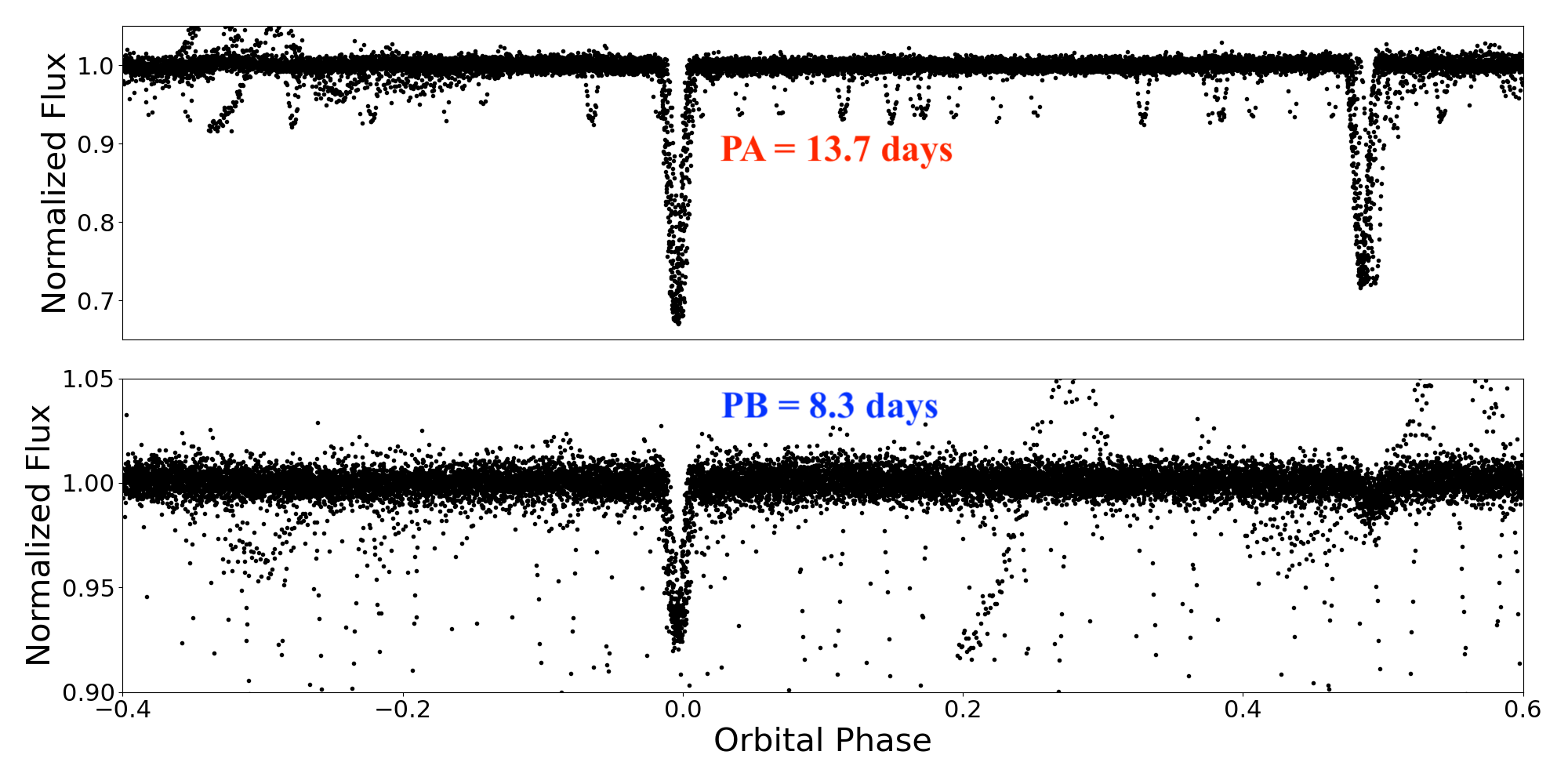
Figure 3: Phase-folded TESS eleanor data on the two periods of PA = 13.65 days (upper panel) and PB = 8.3 days (lower panel), highlighting the deviations from linear ephemeris for both binaries.

Figure 4: Phase-folded ASAS-SN (upper panel) and ATLAS (lower panel) data for TIC 219006972. The PA = 13.65-day eclipses are clearly seen in both the ASAS-SN and the ATLAS photometry, and demonstrate that there are no drastic changes in the PA binary between TESS and ASAS-SN/ATLAS.

Second, detailed investigation of the motion of the center-of-light during the two sets of eclipses confirmed that they originate from the target (see Figure 5), in line with its isolated nature, further strengthening the quadruple hypothesis.

Next, a preliminary analysis of the TESS lightcurve revealed prominent non-linear and correlated Eclipse Timing Variations (ETVs) with a large total amplitude of about 0.1 days (see the upper panel of Fig. 6). In order to check for any obvious periodicity in the ETV curves we carried out $\chi^{2}$ fits using simple sinusoids with a large set of oversampled periods. While most ETV curves, due to either Light Travel Time Effects (LTTE) or dynamical delays (see Sect. 3), are distinctly non-sinusoidal, the dominant Fourier component is still either at the orbital period or its half period—so this is a useful first check for any periodicity. The bottom panel in Fig. 6 shows the resultant $\chi^{2}$ value vs. the trial orbital period when fitting these sinusoids to the ETV curve above. The deepest $\chi^{2}$ minimum (best fit) comes at $P_{\rm out}=169.3\pm 2$ days. The next deepest minimum, at 169/2 days, represents a higher harmonic of $P_{\rm out}$, and can be ruled out as the most significant minimum at the 5-$\sigma$ level. The third deepest minimum occurs at a period of 96 days and is excluded as the most significant minimum at the 7-$\sigma$ level. Thus, we tentatively conclude that the outer period of this quadruple is 169 days, which would comprise the shortest outer orbital period for a published quadruple star system. For a much more comprehensive analysis of the system and derivation of its stellar and orbital parameters we employed a detailed photometric-dynamical model as described in the next section.

Figure 5: Difference images showing center-of-light measurements for PA (left) and PB (right) during the detected eclipses in Sector 41. The star symbols represent the catalog position of the target, the small red dots represent the individual center-of-light measurements for each detected eclipses, the large red circle represents their average, and the dashed white contour represents the pixel aperture used by Eleanor to extract the lightcurve. The measurements confirm that TIC 219006972 is the source of both PA and PB.

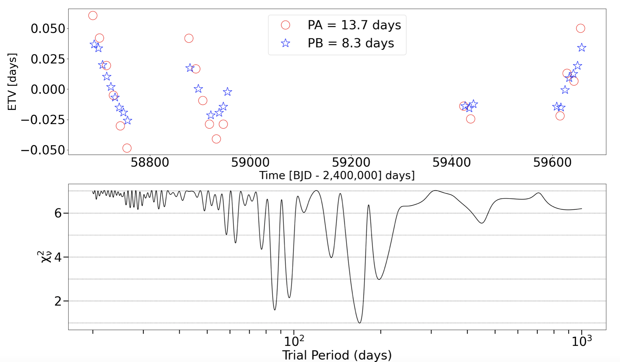
Figure 6: First panel: Preliminary primary ETVs for the PA (red circles) and PB (blue stars) binaries based on the eleanor lightcurve showing clear, correlated deviations from a linear ephemeris. Second panel: $\chi^{2}$ fits to the measured ETVs using simple sinusoids with a large set of oversampled periods. This indicates an initial estimate for the outer period of 169 days.

3 Photodynamical analysis of the system

We carried out a simultaneous, joint analysis of the TESS lightcurve, the ETV curves derived from the mid-times of the TESS-observed eclipses, and the available multi-passband SED data of the system with the Lightcurvefactory software package (Borkovits et al., 2019, 2020). During the analysis we followed the same steps which were described in detail in our previous analysis of TIC 454140642 (Kostov et al., 2021), another TESS-discovered compact quadruple system. The only fundamental difference between the two studies is, that in contrast to this latter system, no Radial Velocity (RV) observations are available for TIC 219006972 and, hence, we were not able to fit RV curve(s) simultaneous to the other parts of the analysis. For further details on the photodynamical analysis we refer the reader to Sect. 5.1 of Kostov et al. (2021). Here, we describe only the data preparation steps which are specific for this system.

As mentioned previously, TIC 219006972 was observed in six sectors during Year 2, and three sectors during Year 4 observations. For the photodynamical analysis we extracted 30-min and 10-min cadenced lightcurves from the FFI files with the Fitsh package (Pál, 2012). We carried out low-order polynomial detrending on the out-of-eclipse sections to eliminate the most trivial, instrumental systematics. Finally, to reduce the computational time, we removed the out-of-eclipse lightcurve sections, keeping only narrow, $\pm 0\@fp 05$-phase-domain regions centered on each eclipse.

Table 2: Mid-eclipse Times for TIC 219006972A

BJD	Cycle	std. dev.	BJD	Cycle	std. dev.	BJD	Cycle	std. dev.	BJD	Cycle	std. dev.
$-2\,400\,000$	no.	$(d)$	$-2\,400\,000$	no.	$(d)$	$-2\,400\,000$	no.	$(d)$	$-2\,400\,000$	no.	$(d)$
58686.282316	0.0	0.000852	58747.534495	4.5	0.000765	58925.077543	17.5	0.000700	59608.037828	67.5	0.000547
58692.978462	0.5	0.000756	58754.466837	5.0	0.000829	58932.035148	18.0	0.000672	59614.985457	68.0	0.000332
58699.923404	1.0	0.000823	58761.184269	5.5	0.000560	58938.733397	18.5	0.000521	59628.679520	69.0	0.000390
58706.618686	1.5	0.000500	58870.515620	13.5	0.001813	58945.707518	19.0	0.000737	59635.372093	69.5	0.000229
58713.559120	2.0	0.000512	58877.484039	14.0	0.000571	58952.406999	19.5	0.000854	59642.331523	70.0	0.000275
58720.255316	2.5	0.000699	58891.118605	15.0	0.000641	59423.772646	54.0	0.000358	59649.047233	70.5	0.000263
58727.193553	3.0	0.000734	58904.752666	16.0	0.000414	59430.453162	54.5	0.000328	59656.033032	71.0	0.000287
58733.894683	3.5	0.000504	58911.431342	16.5	0.000675	59437.421320	55.0	0.000283	59662.792741	71.5	0.000267
58740.828295	4.0	0.000701	58918.389326	17.0	0.000616	59444.119502	55.5	0.000256

Table 3: Mid-Eclipse Times for TIC 219006972B

BJD	Cycle	std. dev.	BJD	Cycle	std. dev.	BJD	Cycle	std. dev.	BJD	Cycle	std. dev.
$-2\,400\,000$	no.	$(d)$	$-2\,400\,000$	no.	$(d)$	$-2\,400\,000$	no.	$(d)$	$-2\,400\,000$	no.	$(d)$
58685.236288	-0.5	0.002285	58738.971483	6.0	0.001241	58917.007916	27.5	0.002995	59608.349704	111.0	0.000646
58689.344931	0.0	0.000406	58743.145273	6.5	0.005062	58921.123356	28.0	0.000697	59612.434059	111.5	0.004515
58693.513113	0.5	0.002803	58747.245300	7.0	0.000273	58925.309371	28.5	0.154352	59616.629119	112.0	0.000224
58697.620699	1.0	0.000559	58755.521954	8.0	0.000379	58929.397837	29.0	0.000447	59620.719734	112.5	0.001450
58705.889871	2.0	0.000448	58871.491234	22.0	0.000353	58937.682106	30.0	0.000301	59624.922346	113.0	0.000276
58710.059326	2.5	0.002269	58875.649635	22.5	0.001726	58945.969802	31.0	0.000576	59628.996033	113.5	0.001859
58714.159819	3.0	0.000940	58879.761833	23.0	0.000331	58954.259163	32.0	0.000233	59633.211735	114.0	0.000251
58718.323564	3.5	0.003754	58888.031673	24.0	0.000305	59422.031984	88.5	0.001088	59641.495204	115.0	0.000229
58722.424307	4.0	0.010602	58892.185449	24.5	0.008371	59426.196701	89.0	0.000479	59645.588546	115.5	0.004204
58726.600576	4.5	0.001527	58896.303106	25.0	0.000371	59434.474604	90.0	0.000371	59649.777672	116.0	0.000209
58730.699461	5.0	0.000258	58900.453999	25.5	0.003658	59438.564007	90.5	0.002448	59658.080745	117.0	0.000253
58734.876726	5.5	0.008773	58908.734092	26.5	0.006369	59442.759324	91.0	0.000355	59662.180871	117.5	0.001639

Additionally, we used the four ETV curves (primary and secondary ETV data for both binaries; see Tables 2 and 3). Furthermore, the observed passband magnitudes tabulated in Table 1 were also used for the SED analysis. Similar to our previous works, for the SED analysis we used a minimum uncertainty of $0.03$ mag for most of the observed passband magnitudes, in order to avoid the outsized contribution of the extremely precise Gaia magnitudes and also to counterbalance the uncertainties inherent in our interpolation method during the calculations of theoretical passband magnitudes that are part of the fitting process. The two exceptions are the WISE $W4$ and GALEX $FUV$ magnitudes, for which the uncertainties were inflated to 0.3 mag.

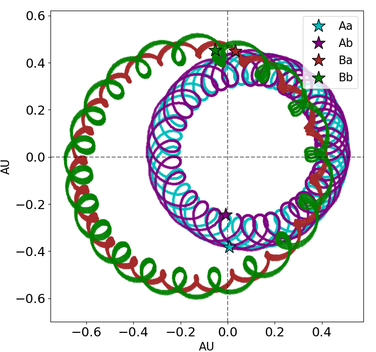
Figure 10: Orbital configuration of TIC 219006972 as seen from above over the course of a few outer periods. The individual components are color-coded as in Fig. 9, i.e. cyan, purple, brown and green lines for Aa, Ab, Ba, and Bb, respectively. The observer is in the x-y plane, looking along the x = 0 direction. The orbits appear thick due to slow orbital precession.

Table 4 lists the median values of the stellar and orbital parameters of the quadruple system that are being either adjusted, internally constrained, or derived from the MCMC posteriors, together with the corresponding $1\sigma$ statistical uncertainties. The ETV curves, sections of the lightcurves, and the SED model of the lowest $\chi^{2}_{\mathrm{global}}$ solution are plotted in Figs. 7, 8, and 9, respectively. The orbital configuration of the system, as seen from above the plane of the outer orbit, is shown in Figure 10 for a few outer periods.

Figure 7: Photodynamical solution for eclipse timing variations of TIC 219006972 showing the best-fit model and corresponding residuals (top panel for binary A, bottom panel for binary B). The red and blue symbols denote the measured primary and secondary ETVs, respectively, while the thin red and blue dots, connected with straight lines, represent the corresponding model. The thin black curves represent the LTTE contributions to the ETVs. As clearly seen from the figure, the dynamical perturbations completely dominate the measured eclipse times.

Figure 8: Example sections of the TESS lightcurve (blue points) along with the best-fit model (red) and the corresponding residuals. The upper panel represents a continuous, 9-day-long section of the TESS lightcurve. Here the pale blue points (and the corresponding orange residual points) show those out-of-eclipse data (and their residuals) which were not used for the photodynamical analysis. The lower panel represent three different sections of the lightcurve for a beter view of the four different kind of eclipses.

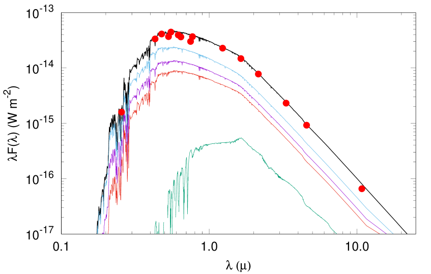
Figure 9: The summed SED of the four stars of TIC 219006972. The dereddened observed magnitudes are converted into the flux domain (red filled circles), and overplotted with the quasi-continuous summed SED for the quadruple star system (thick black line). This SED is computed from the Castelli & Kurucz (2003) ATLAS9 stellar atmospheres models (http://www.user.oats.inaf.it/castelli/grids/gridp00k2odfnew/fp00k2tab.html). The separate SEDs of the four stars (from components Aa, Ab, Ba, and Bb) are also shown with thin cyan, purple, brown and green lines, respectively.

Table 4: Median values of the parameters from the double EB simultaneous lightcurve, double ETV, joint SED and PARSEC evolutionary track solution from Lightcurvefactory.

Orbital elementsa
	subsystem
	A		B		A–B
$P_{\mathrm{a}}$ [days]	$13.6389_{-0.0024}^{+0.0025}$		$8.23247_{-0.00049}^{+0.00050}$		$168.187_{-0.071}^{+0.069}$
semimajor axis [$R_{\odot}$]	$29.69_{-0.66}^{+0.67}$		$18.84_{-0.33}^{+0.38}$		$189.2_{-3.9}^{+4.2}$
$i$ [deg]	$89.45_{-0.12}^{+0.20}$		$89.53_{-0.39}^{+0.32}$		$88.52_{-0.45}^{+0.38}$
$e$	$0.01518_{-0.00026}^{+0.00026}$		$0.01847_{-0.00066}^{+0.00070}$		$0.2543_{-0.0023}^{+0.0022}$
$\omega$ [deg]	$303.40_{-0.72}^{+0.70}$		$260.09_{-0.99}^{+1.00}$		$16.19_{-0.73}^{+0.74}$
$\tau^{b}$ [BJD]	$2\,458\,673.8396_{-0.0269}^{+0.0259}$		$2\,458\,689.0956_{-0.0221}^{+0.0223}$		$2\,458\,639.250_{-0.409}^{+0.415}$
$\Omega$ [deg]	$0.0$		$-0.26_{-0.67}^{+0.98}$		$-0.62_{-0.35}^{+0.28}$
$(i_{\mathrm{m}})_{A-...}^{c}$ [deg]	$0.0$		$0.80_{-0.33}^{+0.39}$		$1.12_{-0.45}^{+0.64}$
$(i_{\mathrm{m}})_{B-...}$ [deg]	$0.80_{-0.33}^{+0.39}$		$0.0$		$1.31_{-0.47}^{+0.72}$
$\varpi_{\mathrm{dyn}}^{d}$ [deg ]	$123.40_{-0.72}^{+0.70}$		$80.10_{-0.99}^{+1.00}$		$196.18_{-0.73}^{+0.74}$
$i_{\mathrm{dyn}}^{d}$ [deg]	$0.88_{-0.37}^{+0.53}$		$1.08_{-0.42}^{+0.60}$		$0.25_{-0.09}^{+0.12}$
$\Omega_{\mathrm{dyn}}^{d}$ [deg]	$213.70_{-7.00}^{+4.43}$		$202.31_{-41.98}^{+35.04}$		$30.27_{-11.31}^{+11.89}$
$i_{\mathrm{inv}}^{e}$ [deg]	$88.72_{-0.35}^{+0.31}$
$\Omega_{\mathrm{inv}}^{e}$ [deg]	$-0.49_{-0.29}^{+0.24}$
mass ratio $[q=m_{\mathrm{sec}}/m_{\mathrm{pri}}]$	$0.931_{-0.005}^{+0.005}$		$0.563_{-0.026}^{+0.023}$		$0.705_{-0.010}^{+0.012}$
$K_{\mathrm{pri}}$ [km s-1]	$53.1_{-1.1}^{+1.1}$		$41.6_{-1.2}^{+1.4}$		$24.3_{-0.4}^{+0.5}$
$K_{\mathrm{sec}}$ [km s-1]	$57.1_{-1.4}^{+1.3}$		$74.1_{-1.6}^{+2.0}$		$34.6_{-0.9}^{+0.7}$
Apsidal and nodal motion related parametersf
$P_{\mathrm{apse}}$ [year]	$16.59_{-0.13}^{+0.13}$		$19.35_{-0.14}^{+0.17}$		$59.54_{-0.44}^{+0.42}$
$P_{\mathrm{apse}}^{\mathrm{dyn}}$ [year]	$7.57_{-0.05}^{+0.05}$		$9.29_{-0.06}^{+0.07}$		$13.74_{-0.09}^{+0.10}$
$P_{\mathrm{node}}^{\mathrm{dyn}}$ [year]	$13.92_{-0.07}^{+0.08}$		$17.86_{-0.13}^{+0.12}$
$\Delta\omega_{\mathrm{3b}}^{\mathrm{dyn}}$ [arcsec/cycle]	$6391_{-40}^{+45}$		$3144_{-25}^{+21}$		$43426_{-303}^{+284}$
$\Delta\omega_{\mathrm{GR}}$ [arcsec/cycle]	$0.53_{-0.02}^{+0.02}$		$0.58_{-0.02}^{+0.02}$		$0.150_{-0.006}^{+0.007}$
$\Delta\omega_{\mathrm{tide}}$ [arcsec/cycle]	$0.097_{-0.003}^{+0.003}$		$0.103_{-0.011}^{+0.017}$		$-$
Stellar parameters
	Aa	Ab	Ba	Bb
Relative quantities
fractional radius [$R/a$]	$0.0380_{-0.0004}^{+0.0004}$	$0.0318_{-0.0005}^{+0.0005}$	$0.0441_{-0.0012}^{+0.0018}$	$0.0246_{-0.0010}^{+0.0014}$
fractional flux [in TESS-band]	$0.468_{-0.023}^{+0.019}$	$0.287_{-0.008}^{+0.012}$	$0.195_{-0.016}^{+0.021}$	$0.011_{-0.001}^{+0.002}$
Physical Quantities
$m$ [M⊙]	$0.977_{-0.065}^{+0.069}$	$0.908_{-0.058}^{+0.061}$	$0.846_{-0.045}^{+0.054}$	$0.475_{-0.024}^{+0.032}$
$R^{g}$ [R⊙]	$1.128_{-0.022}^{+0.020}$	$0.943_{-0.035}^{+0.034}$	$0.831_{-0.031}^{+0.047}$	$0.464_{-0.025}^{+0.033}$
$T_{\mathrm{eff}}^{g}$ [K]	$6162_{-100}^{+85}$	$5942_{-94}^{+75}$	$5676_{-95}^{+123}$	$3698_{-45}^{+51}$
$L_{\mathrm{bol}}^{g}$ [L⊙]	$1.643_{-0.149}^{+0.154}$	$0.993_{-0.124}^{+0.131}$	$0.642_{-0.083}^{+0.139}$	$0.036_{-0.005}^{+0.008}$
$M_{\mathrm{bol}}^{g}$	$4.23_{-0.10}^{+0.10}$	$4.78_{-0.13}^{+0.14}$	$5.25_{-0.21}^{+0.15}$	$8.38_{-0.21}^{+0.15}$
$M_{V}^{g}$	$4.26_{-0.11}^{+0.11}$	$4.83_{-0.15}^{+0.16}$	$5.34_{-0.23}^{+0.17}$	$9.70_{-0.25}^{+0.19}$
$\log g^{g}$ [dex]	$4.322_{-0.018}^{+0.015}$	$4.446_{-0.007}^{+0.007}$	$4.523_{-0.023}^{+0.018}$	$4.780_{-0.032}^{+0.025}$
Global Quantities
$\log$(age)g [dex]	$9.779_{-0.172}^{+0.142}$
$[M/H]^{g}$ [dex]	$-0.275_{-0.082}^{+0.070}$
$E(B-V)$ [mag]	$0.048_{-0.026}^{+0.020}$
$(M_{V})_{\mathrm{tot}}^{g}$	$3.52_{-0.13}^{+0.13}$
distance [pc]	$1327_{-45}^{+50}$

Notes. (a) Instantaneous, osculating orbital elements at epoch $t_{0}=2\,458325.0$; (b) Time of periastron passsage; (c) Mutual (relative) inclination; (d) Longitude of pericenter ($\varpi_{\mathrm{dyn}}$) and inclination ($i_{\mathrm{dyn}}$) with respect to the dynamical (relative) reference frame (see text for details); (e) Inclination ($i_{\mathrm{inv}}$) and node ($\Omega_{\mathrm{inv}}$) of the invariable plane to the sky; (f) See Sect 4.1 for a detailed discussion of the tabulated apsidal motion parameters; (g) Interpolated from the PARSEC isochrones;

4 Discussion

4.1 System properties

According to the results of our photodynamical analysis of the TIC 219006972 system, the longer period binary A is formed by two similar Sun-like stars with masses $m_{\mathrm{Aa}}=0.98\pm 0.07\,\mathrm{M}_{\odot}$ and $m_{\mathrm{Ab}}=0.91\pm 0.06\,\mathrm{M}_{\odot}$, respectively. We note that the relatively large (6-7%) uncertainties in the masses are a consequence of the lack of RV measurements. In the absence of such data, the absolute masses of the stars are constrained only by (i) the dynamical perturbations through the eclipse timings and, (ii) the combinations of PARSEC isochrones and cumulative SED fittings, as described and discussed in detail in Borkovits et al. (2022). The mass ratio of binary A, however, is much better constrained to $q_{\mathrm{A}}=0.931\pm 0.005$. In contrast, the shorter period binary B consists of two less massive, largely unequal mass stars ($q_{\mathrm{B}}=0.56\pm 0.02$). The primary in binary B is a $m_{\mathrm{Ba}}=0.85\pm 0.05\,\mathrm{M}_{\odot}$ late G-type star, and the secondary is a smaller, $m_{\mathrm{Bb}}=0.48\pm 0.03\,\mathrm{M}_{\odot}$ red dwarf. The best-fit solution implies that the quadruple system is most likely moderately metal deficient relative to the Sun $[M/H]=-0.28\pm 0.08$, and has an age of $\tau=6\pm 2$ Gyr-old.

The most remarkable property of TIC 219006972 is its very tight and compact orbital configuration. Hence, in what follows, we investigate this property in detail. Specifically, we discuss the current dynamical and observational implications of the system’s configuration and evaluate its long-term dynamical stability.

According to our results the system is quite flat – none of the three mutual inclination angles amongst orbital planes A, B and AB exceeds 2°(within the corresponding $1\sigma$ uncertainties). These findings are in accord with the fact that the deeper-eclipses of binary A were also detected in the ASAS-SN and ATLAS data (see Fig. 6). Thus, one can exclude the possibility of large amplitude orbital plane precession and the corresponding rapid disappearance of the eclipses. The characteristic nodal precession timescale of $P_{\mathrm{node}}=13.9\pm 0.1$ yr (see also Table 4), would cause the eclipse depths to change noticeably even over the decade spanned by the ATLAS and ASAS-SN data.

While we cannot detect precession of the orbital plane, the strong dynamical perturbations manifest themselves via at least two prominent observable effects. First, the ETV curves of both binaries exhibit 1-2 h amplitude quasi-sinusoidal variations with the outer period of $P_{\mathrm{out}}=168$ d (upper panels of Fig. 7). These quasi-sinusoidal cycles, which are in phase for both binaries and operate on a medium ($P_{\mathrm{out}}$)-timescale, are manifestations of the perturbations of each binary due to the Keplerian motion of the other (see, e.g. Borkovits et al., 2015). We note that these should not be confused with the purely geometrical LTTE, which follows a similar period but produces strictly anticorrelated ETVs for the two binaries, and has only a minor contribution to the measured ETVs.

The other prominent perturbation effect is the rapid, dynamically-forced apsidal motion, which manifests itself in the divergent behaviour of the primary (red) and secondary (blue) ETV curves. Table 4 provides the theoretical apsidal motion periods both in the observational and the dynamical frame of reference. The predicted apsidal motion periods in the observational frame of reference for the two binaries are $P_{\mathrm{apsidal,A}}=16.6\pm 0.1$ yr and $P_{\mathrm{apsidal,B}}=19.4\pm 0.2$ yr. Besides these, we also list the cycle by cycle angular contribution of the classic tidal, general relativistic and the dynamical third (fourth) body effects to the advance of the (dynamical) argument of pericenter. As seen from the table, the effect of the dynamical perturbations of each binary to the other completely dominates the relativistic and the classic tidal apsidal motion effects.

Similar to the two eclipsing pairs, the outer orbital plane was also found to be very close to a perfectly edge-on view ($i_{\mathrm{out}}=88.5\arcdeg\pm 0.4\arcdeg$), raising the interesting question whether TIC 219006972 produces mutual eclipses. Using the best-fit parameters and numerical simulations, we calculated the impact parameters between each star from each binary with respect to each star from the other binary. As demonstrated in Figure 11, our results show that the mutual impact parameters do not reach below 2 for the duration of the integrations, indicating that the two binaries barely miss each other on-sky and suggesting that mutual inclinations are unlikely in the near future.

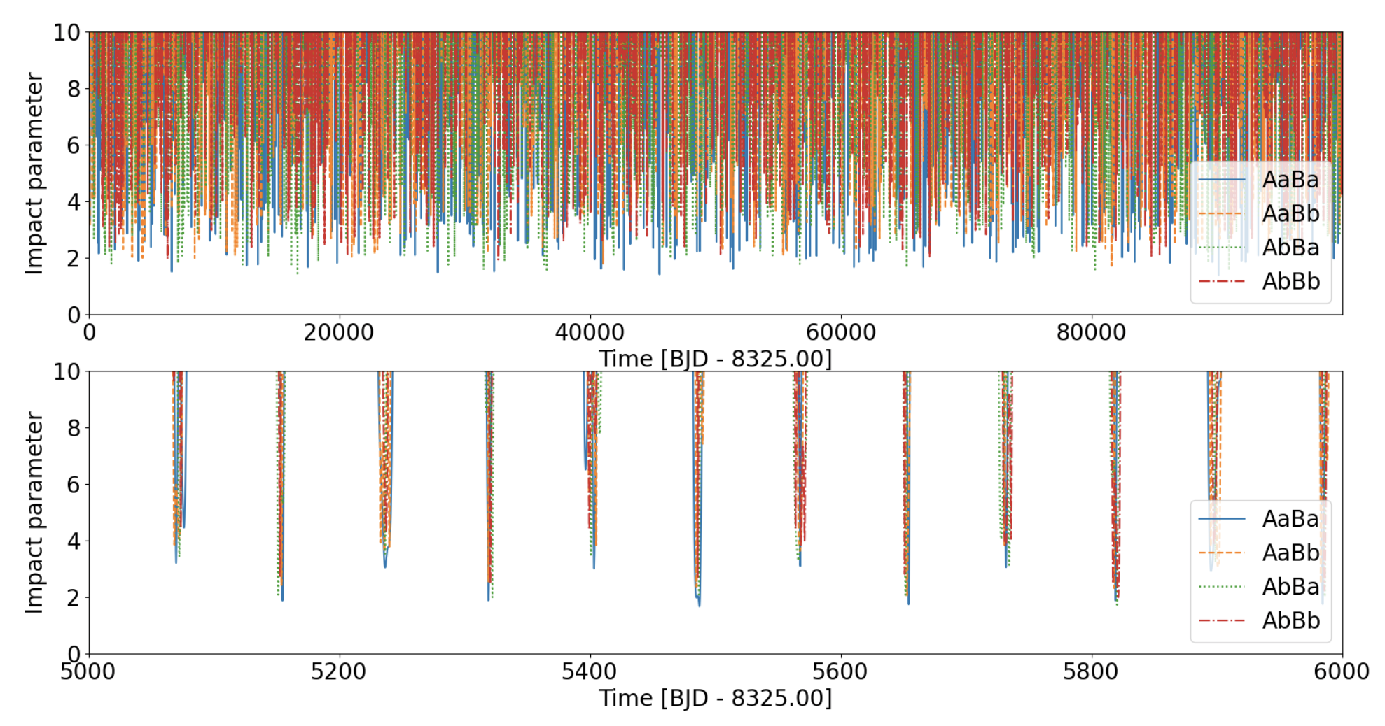
Figure 11: Upper panel: Evolution of the separation between stellar centers of each star of one binary with radius $R_{i}$, with respect to each star of the other binary with radius $R_{j}$ in units of $R_{i}+R_{j}$ (i.e., the ‘impact parameters’) over the course of 100,000 days. For example, AaBb represents the impact parameter between the primary star of binary A with respect to the secondary star of binary B. When the impact parameter is $<1$ there is a corresponding eclipse. Lower panel: same as upper panel but zoomed-in on a period of 1,000 days.

4.2 Origin

Multiple stars form through two main channels: (i) fragmentation of cores and filaments of molecular clouds on large (0.01–0.1 pc) scales and (ii) fragmentation of gravitationally unstable protostellar disks at smaller (10–500 AU) separations (see Offner et al., 2022, for a review). Dynamical friction, disk capture, and circumbinary disk accretion can drive the binary orbits to shorter separations. For example, compact coplanar triples, such as the majority of Kepler EBs exhibiting eclipse timing variations (Borkovits et al., 2016), likely formed via two successive episodes of disk fragmentation and inward disk migration (Tobin et al., 2016; Tokovinin & Moe, 2020). However, not all compact triples survive the embedded protostellar stage as some inner binaries may migrate too far in and merge, and some outer tertiaries may migrate into the dynamical instability regime, leading to an ejection of one of the components.

Although multiple episodes of disk fragmentation and migration can create compact triples and even (2+1)+1 quadruples, disk fragmentation alone cannot readily produce 2+2 quadruples. Instead, compact 2+2 quadruples likely first derived from core fragmentation on wider scales. Both resulting cores subsequently collapsed into protostellar disks and fragmented again to create the inner companions. Disk fragmentation and inward disk migration can harden binaries down to $P$ $\approx$ 1 day (Moe & Kratter, 2018; Tokovinin & Moe, 2020), but the processes of core fragmentation and subsequent dynamical friction tend to leave binaries in slightly larger orbits. Hence, the most compact triple, $\lambda$ Tau at $P_{\rm out}$ = 33 days, is substantially tighter than the most compact 2+2 quadruple presented here, TIC 219006972 with $P_{\rm out}$ = 168 days.

In their toy model of disk fragmentation, accretion, and migration, Tokovinin & Moe (2020) successfully reproduced the short-end tail of the solar-type binary period distribution (see their Fig. 4). Beyond $P$ $>$ 100 days, however, their simulated population underpredicted the observed rate, suggesting other formation mechanisms, e.g., core fragmentation begins to contribute at these wider separations. This newly discovered compact quadruple is just beyond the expected transition. Moreover, TIC 219006972 provides some of the strongest evidence that solar-type multiples that initially formed via core fragmentation on $\sim$ 10,000 AU scales can migrate all the way down to $\sim$ 1 AU.

4.3 Dynamical Stability and Orbital Evolution

Given there are two binary stars with a total mass of about 3 ${M_{\odot}}$ orbiting each other within less than 1 AU (0.877 AU at pericenter), it is quite interesting and instructive to evaluate the long-term stability and orbital evolution of the system. Moreover, we point out that this system is quite ‘tight’, i.e., with small ratios of $P_{\rm out}/P_{\rm in}\simeq 12.3$ and 20.4 for the A and B binaries, respectively. To check on the system stability, we first use the analytic fitting formalae of Mardling & Aarseth (2001) to calculate the critical semi-major axis and period of the quadruple (below which the system would tend to be dynamically unstable). From Eqn. (16) of Rappaport et al. (2013), the latter must be ${\rm P_{quadruple}>135~{}days}$. This is formally below the actual period of 168 days, suggesting that the system is indeed long-term stable and worthy of numerical investigations.

Therefore, we performed N-body simulations based on the best-fit parameters from the photodynamical solution using the REBOUND package (Rein & Liu, 2012). An example from these simulations is shown in Figure 12 for the case of dynamical integrations spanning 168,000 days ($\approx$1,000 outer orbits). As seen from the figure, the orbital elements of each of the two binaries and the quadruple itself oscillate around their respective mean values without any indications of chaotic behavior for the duration of the integrations. As highlighted in Figure 13, numerical simulations extending to 1 million days (about 6,000 outer orbits) confirm that the system to exhibit the same behavior as seen in the shorter integration. The semi-major axes of the two binaries oscillate by no more than 2.5% and the corresponding eccentricities reach no higher than about 0.05; the semi-major of the quadruple varies between 0.877 AU and 0.889 AU, and its eccentricity varies between 0.247 and 0.266.

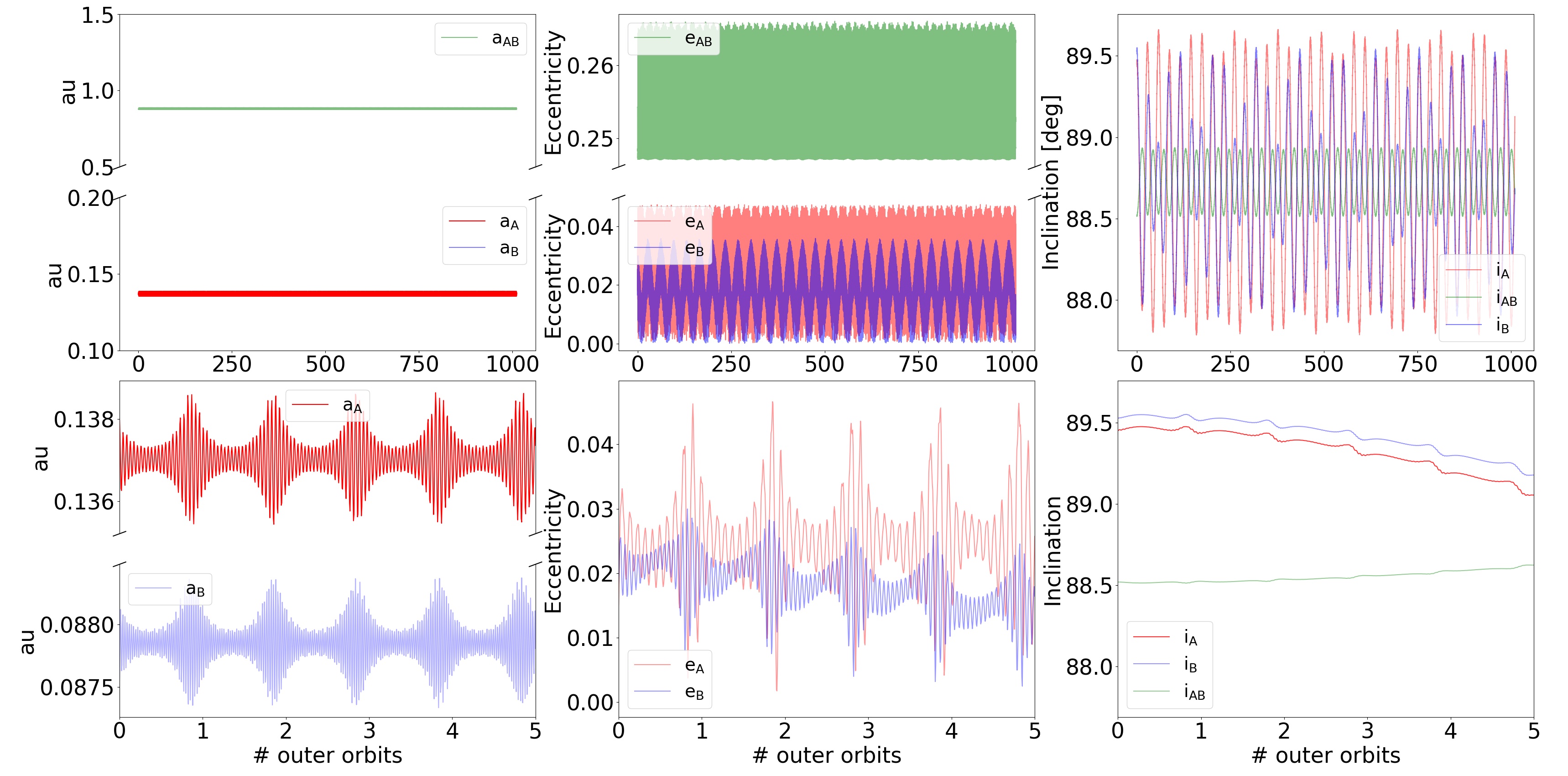
Figure 12: Dynamical evolution of the system shows no signs of chaotic motion. The first column represents the evolution of the three semi-major axes as a function of the outer orbit number, the second column represents the evolution of the three orbital eccentricities and the third columns represents the evolution of the three inclinations. The upper row shows the evolution over the course of 1,000 outer orbits ($\approx$168,000 days) and the lower row shows the evolution over the course of 5 outer orbits. The strong effect of the outer periastron passage on the orbital elements of the two binaries is clearly seen in the lower panels.

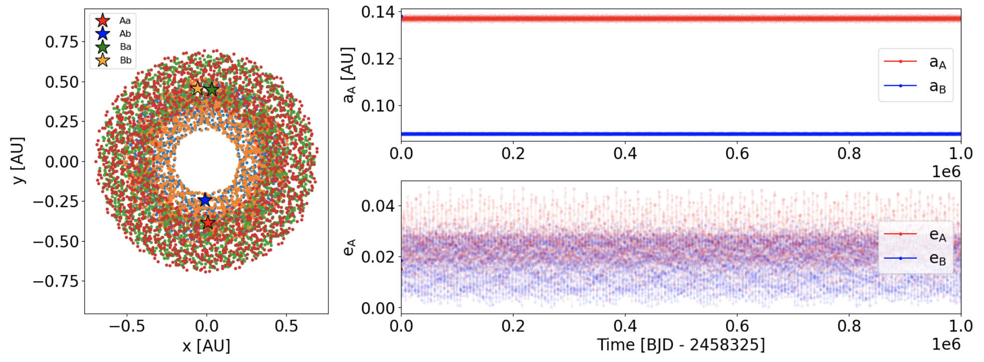
Figure 13: Numerical integrations of the system for 1 million days using the best-fit photodynamical parameters. Left: Orbital configuration of the system. Right panels: Evolution of the semi-major axes (upper) and eccentricities (lower panels) of the two binaries. The system remains stable for the duration of the integrations.

We note that since our numerical simulations cover only a tiny fraction of the system’s lifetime, it would be interesting to integrate the TIC 219006972 system for a substantial amount of time ($10^{6}-10^{9}$ years) and probe its long-term dynamics. This would be instructive to do since the system is somewhat close to its dynamical stability limit. Of course, the bottom line is that at least we know the system is empirically stable on Gyr timescales since its age is $6\pm 2$ Gyr old.

5 Summary

In this work, we have presented the discovery of TIC 219006972 – a compact, eclipsing, nearly co-planar quadruple star producing two sets of primary and secondary eclipses in TESS data. The two eclipsing binaries have orbital periods of PA = 13.7 days and PB = 8.3 days, respectively, rather small eccentricities (about 0.02), and orbit each other every 168 days on a slightly eccentric outer orbit ($e_{\mathrm{out}}=0.25$). This makes TIC 219006972 the shortest-period quadruple system reported to date, and the second closest to co-planarity.

The masses of the component stars range from 0.48 $M_{\odot}$ to 0.98 $M_{\odot}$, their radii from 0.46 $R_{\odot}$ to 1.13 $R_{\odot}$, and the respective effective temperatures from 3698 K to 6162 K. The systems is slightly metal-deficient ([M/H] = -0.28), has an age of about 6 Gyr, and appears empirically to be long-term dynamically stable – in agreement with the analytic stability formalism of Mardling & Aarseth (2001).

TIC 219006972 raises some intriguing questions such as (i) are there quadruples with substantially shorter outer periods, e.g., $\lesssim 100$ days, and (ii) is there a fundamental lower limit below which quadruples simply cannot form? With the continued operation of the TESS and Gaia missions, we hope to further explore these questions.

6 Data Availability

The data underlying this article will be shared on reasonable request to the corresponding author.

References

- Abadi et al. (2015) Abadi, M., Agarwal, A., Barham, P., et al. 2015, TensorFlow: Large-Scale Machine Learning on Heterogeneous Systems. https://www.tensorflow.org/
- Aller et al. (2020) Aller, A., Lillo-Box, J., Jones, D., Miranda, L. F., & Barceló Forteza, S. 2020, A&A, 635, A128, doi: 10.1051/0004-6361/201937118
- Astropy Collaboration et al. (2013) Astropy Collaboration, Robitaille, T. P., Tollerud, E. J., et al. 2013, A&A, 558, A33, doi: 10.1051/0004-6361/201322068
- Astropy Collaboration et al. (2018) Astropy Collaboration, Price-Whelan, A. M., Sipőcz, B. M., et al. 2018, AJ, 156, 123, doi: 10.3847/1538-3881/aabc4f
- Borkovits (2022) Borkovits, T. 2022, Galaxies, 10, 9, doi: 10.3390/galaxies10010009
- Borkovits et al. (2016) Borkovits, T., Hajdu, T., Sztakovics, J., et al. 2016, MNRAS, 455, 4136, doi: 10.1093/mnras/stv2530
- Borkovits et al. (2015) Borkovits, T., Rappaport, S., Hajdu, T., & Sztakovics, J. 2015, MNRAS, 448, 946, doi: 10.1093/mnras/stv015
- Borkovits et al. (2020) Borkovits, T., Rappaport, S. A., Hajdu, T., et al. 2020, MNRAS, 493, 5005, doi: 10.1093/mnras/staa495
- Borkovits et al. (2019) Borkovits, T., Rappaport, S., Kaye, T., et al. 2019, MNRAS, 483, 1934, doi: 10.1093/mnras/sty3157
- Borkovits et al. (2022) Borkovits, T., Mitnyan, T., Rappaport, S. A., et al. 2022, MNRAS, 510, 1352, doi: 10.1093/mnras/stab3397
- Burke et al. (2020) Burke, C. J., Levine, A., Fausnaugh, M., et al. 2020, TESS-Point: High precision TESS pointing tool, Astrophysics Source Code Library. http://ascl.net/2003.001
- Castelli & Kurucz (2003) Castelli, F., & Kurucz, R. L. 2003, in Modelling of Stellar Atmospheres, ed. N. Piskunov, W. W. Weiss, & D. F. Gray, Vol. 210, A20, doi: 10.48550/arXiv.astro-ph/0405087
- Chollet et al. (2015) Chollet, F., et al. 2015, Keras, https://keras.io
- Cutri et al. (2012) Cutri, R. M., Wright, E. L., Conrow, T., et al. 2012, Explanatory Supplement to the WISE All-Sky Data Release Products, Explanatory Supplement to the WISE All-Sky Data Release Products
- Dalcin et al. (2008) Dalcin, L., Paz, R., Storti, M., & D’Elia, J. 2008, Journal of Parallel and Distributed Computing, 68, 655, doi: http://dx.doi.org/10.1016/j.jpdc.2007.09.005
- De Rosa et al. (2014) De Rosa, R. J., Patience, J., Wilson, P. A., et al. 2014, MNRAS, 437, 1216, doi: 10.1093/mnras/stt1932
- Ebbighausen & Struve (1956) Ebbighausen, E. G., & Struve, O. 1956, ApJ, 124, 507, doi: 10.1086/146254
- Fang et al. (2018) Fang, X., Thompson, T. A., & Hirata, C. M. 2018, MNRAS, 476, 4234, doi: 10.1093/mnras/sty472
- Feinstein et al. (2019) Feinstein, A. D., Montet, B. T., Foreman-Mackey, D., et al. 2019, PASP, 131, 094502, doi: 10.1088/1538-3873/ab291c
- Fragione & Kocsis (2019) Fragione, G., & Kocsis, B. 2019, MNRAS, 486, 4781, doi: 10.1093/mnras/stz1175
- Gaia Collaboration et al. (2021) Gaia Collaboration, Brown, A. G. A., Vallenari, A., et al. 2021, A&A, 649, A1, doi: 10.1051/0004-6361/202039657
- Hamers et al. (2021) Hamers, A. S., Rantala, A., Neunteufel, P., Preece, H., & Vynatheya, P. 2021, MNRAS, 502, 4479, doi: 10.1093/mnras/stab287
- Harris et al. (2020) Harris, C. R., Millman, K. J., van der Walt, S. J., et al. 2020, Nature, 585, 357, doi: 10.1038/s41586-020-2649-2
- Heinze et al. (2018) Heinze, A. N., Tonry, J. L., Denneau, L., et al. 2018, AJ, 156, 241, doi: 10.3847/1538-3881/aae47f
- Hunter (2007) Hunter, J. D. 2007, Computing in science & engineering, 9, 90
- Kochanek et al. (2017) Kochanek, C. S., Shappee, B. J., Stanek, K. Z., et al. 2017, PASP, 129, 104502, doi: 10.1088/1538-3873/aa80d9
- Kostov et al. (2021) Kostov, V. B., Powell, B. P., Torres, G., et al. 2021, ApJ, 917, 93, doi: 10.3847/1538-4357/ac04ad
- Kostov et al. (2022) Kostov, V. B., Powell, B. P., Rappaport, S. A., et al. 2022, ApJS, 259, 66, doi: 10.3847/1538-4365/ac5458
- Kotikalapudi & contributors (2017) Kotikalapudi, R., & contributors. 2017, keras-vis, https://github.com/raghakot/keras-vis, GitHub
- Kozai (1962) Kozai, Y. 1962, AJ, 67, 591, doi: 10.1086/108790
- Kristiansen et al. (2022) Kristiansen, M. H. K., Rappaport, S. A., Vanderburg, A. M., et al. 2022, PASP, 134, 074401, doi: 10.1088/1538-3873/ac6e06
- Lidov (1962) Lidov, M. L. 1962, Planet. Space Sci., 9, 719, doi: 10.1016/0032-0633(62)90129-0
- Lightkurve Collaboration et al. (2018) Lightkurve Collaboration, Cardoso, J. V. d. M., Hedges, C., et al. 2018, Lightkurve: Kepler and TESS time series analysis in Python, Astrophysics Source Code Library. http://ascl.net/1812.013
- Liu & Lai (2019) Liu, B., & Lai, D. 2019, MNRAS, 483, 4060, doi: 10.1093/mnras/sty3432
- Mardling & Aarseth (2001) Mardling, R. A., & Aarseth, S. J. 2001, MNRAS, 321, 398, doi: 10.1046/j.1365-8711.2001.03974.x
- McKinney (2010) McKinney, W. 2010, in Proceedings of the 9th Python in Science Conference, ed. S. van der Walt & J. Millman, 51 – 56
- Moe & Di Stefano (2017) Moe, M., & Di Stefano, R. 2017, ApJS, 230, 15, doi: 10.3847/1538-4365/aa6fb6
- Moe & Kratter (2018) Moe, M., & Kratter, K. M. 2018, ApJ, 854, 44, doi: 10.3847/1538-4357/aaa6d2
- Naoz & Fabrycky (2014) Naoz, S., & Fabrycky, D. C. 2014, ApJ, 793, 137, doi: 10.1088/0004-637X/793/2/137
- Offner et al. (2022) Offner, S. S. R., Moe, M., Kratter, K. M., et al. 2022, arXiv e-prints, arXiv:2203.10066, doi: 10.48550/arXiv.2203.10066
- Pál (2012) Pál, A. 2012, MNRAS, 421, 1825, doi: 10.1111/j.1365-2966.2011.19813.x
- Pedregosa et al. (2011) Pedregosa, F., Varoquaux, G., Gramfort, A., et al. 2011, Journal of Machine Learning Research, 12, 2825
- Pejcha et al. (2013) Pejcha, O., Antognini, J. M., Shappee, B. J., & Thompson, T. A. 2013, MNRAS, 435, 943, doi: 10.1093/mnras/stt1281
- Perets & Fabrycky (2009) Perets, H. B., & Fabrycky, D. C. 2009, ApJ, 697, 1048, doi: 10.1088/0004-637X/697/2/1048
- Pérez & Granger (2007) Pérez, F., & Granger, B. E. 2007, Computing in Science and Engineering, 9, 21, doi: 10.1109/MCSE.2007.53
- Powell et al. (2021) Powell, B. P., Kostov, V. B., Rappaport, S. A., et al. 2021, AJ, 161, 162, doi: 10.3847/1538-3881/abddb5
- Powell et al. (2022a) Powell, B. P., Rappaport, S. A., Borkovits, T., et al. 2022a, ApJ, 938, 133, doi: 10.3847/1538-4357/ac8934
- Powell et al. (2022b) Powell, B. P., Kruse, E., Montet, B. T., et al. 2022b, Research Notes of the American Astronomical Society, 6, 111, doi: 10.3847/2515-5172/ac74c4
- Pribulla et al. (2008) Pribulla, T., Baluďanský, D., Dubovský, P., et al. 2008, MNRAS, 390, 798, doi: 10.1111/j.1365-2966.2008.13781.x
- Pribulla et al. (2020) Pribulla, T., Puha, E., Borkovits, T., et al. 2020, MNRAS, 494, 178, doi: 10.1093/mnras/staa699
- Raghavan et al. (2010) Raghavan, D., McAlister, H. A., Henry, T. J., et al. 2010, ApJS, 190, 1, doi: 10.1088/0067-0049/190/1/1
- Rappaport et al. (2013) Rappaport, S., Deck, K., Levine, A., et al. 2013, ApJ, 768, 33, doi: 10.1088/0004-637X/768/1/33
- Rappaport et al. (2022) Rappaport, S. A., Borkovits, T., Gagliano, R., et al. 2022, MNRAS, 513, 4341, doi: 10.1093/mnras/stac957
- Rein & Liu (2012) Rein, H., & Liu, S.-F. 2012, Astronomy & Astrophysics, 537, A128
- Ricker et al. (2015) Ricker, G. R., Winn, J. N., Vanderspek, R., et al. 2015, Journal of Astronomical Telescopes, Instruments, and Systems, 1, 014003, doi: 10.1117/1.JATIS.1.1.014003
- Schlesinger (1916) Schlesinger, F. 1916, Publications of the Allegheny Observatory of the University of Pittsburgh, 3, 23
- Schmitt & Vanderburg (2021) Schmitt, A., & Vanderburg, A. 2021, arXiv e-prints, arXiv:2103.10285. https://arxiv.org/abs/2103.10285
- Schmitt et al. (2019) Schmitt, A. R., Hartman, J. D., & Kipping, D. M. 2019, arXiv e-prints, arXiv:1910.08034. https://arxiv.org/abs/1910.08034
- Skrutskie et al. (2006) Skrutskie, M. F., Cutri, R. M., Stiening, R., et al. 2006, AJ, 131, 1163, doi: 10.1086/498708
- Stassun et al. (2018) Stassun, K. G., Oelkers, R. J., Pepper, J., et al. 2018, AJ, 156, 102, doi: 10.3847/1538-3881/aad050
- Sullivan et al. (2015) Sullivan, P. W., Winn, J. N., Berta-Thompson, Z. K., et al. 2015, ApJ, 809, 77, doi: 10.1088/0004-637X/809/1/77
- Tobin et al. (2016) Tobin, J. J., Kratter, K. M., Persson, M. V., et al. 2016, Nature, 538, 483, doi: 10.1038/nature20094
- Tokovinin (2017) Tokovinin, A. 2017, MNRAS, 468, 3461, doi: 10.1093/mnras/stx707
- Tokovinin & Moe (2020) Tokovinin, A., & Moe, M. 2020, MNRAS, 491, 5158, doi: 10.1093/mnras/stz3299
- Toonen et al. (2016) Toonen, S., Hamers, A., & Portegies Zwart, S. 2016, Computational Astrophysics and Cosmology, 3, 6, doi: 10.1186/s40668-016-0019-0
- Virtanen et al. (2020) Virtanen, P., Gommers, R., Oliphant, T. E., et al. 2020, Nature Methods, doi: https://doi.org/10.1038/s41592-019-0686-2
- Zasche et al. (2022) Zasche, P., Henzl, Z., & Mašek, M. 2022, A&A, 664, A96, doi: 10.1051/0004-6361/202243723
- Zasche et al. (2023) Zasche, P., Borkovits, T., Jayaraman, R., et al. 2023, MNRAS, doi: 10.1093/mnras/stad328