DyLiN: Making Light Field Networks Dynamic

Abstract

Light Field Networks, the re-formulations of radiance fields to oriented rays, are magnitudes faster than their coordinate network counterparts, and provide higher fidelity with respect to representing 3D structures from 2D observations. They would be well suited for generic scene representation and manipulation, but suffer from one problem: they are limited to holistic and static scenes. In this paper, we propose the Dynamic Light Field Network (DyLiN) method that can handle non-rigid deformations, including topological changes. We learn a deformation field from input rays to canonical rays, and lift them into a higher dimensional space to handle discontinuities. We further introduce CoDyLiN, which augments DyLiN with controllable attribute inputs. We train both models via knowledge distillation from pretrained dynamic radiance fields. We evaluated DyLiN using both synthetic and real world datasets that include various non-rigid deformations. DyLiN qualitatively outperformed and quantitatively matched state-of-the-art methods in terms of visual fidelity, while being $25-71\times$ computationally faster. We also tested CoDyLiN on attribute annotated data and it surpassed its teacher model. Project page: https://dylin2023.github.io.

1 Introduction

Machine vision has made tremendous progress with respect to reasoning about 3D structure using 2D observations. Much of this progress can be attributed to the emergence of coordinate networks [6, 21, 26], such as Neural Radiance Fields (NeRF) [23] and its variants [2, 22, 39, 20]. They provide an object agnostic representation for 3D scenes and can be used for high-fidelity synthesis for unseen views. While NeRFs mainly focus on static scenes, a series of works[29, 34, 10, 27] extend the idea to dynamic cases via additional components that map the observed deformations to a canonical space, supporting moving and shape-evolving objects. It was further shown that by lifting this canonical space to higher dimensions the method can handle changes in scene topology as well [28].

However, the applicability of NeRF models is considerably limited by their computational complexities. From each pixel, one typically casts a ray from that pixel, and numerically integrates the radiance and color densities computed by a Multi-Layer Perceptron (MLP) across the ray, approximating the pixel color. Specifically, the numerical integration involves sampling hundreds of points across the ray, and evaluating the MLP at all of those locations. Several works have been proposed for speeding up static NeRFs. These include employing a compact 3D representation structure [18, 43, 9], breaking up the MLP into multiple smaller networks [30, 31], leveraging depth information [24, 7], and using fewer sampling points [17, 24, 42]. Yet, these methods still rely on integration and suffer from sampling many points, making them prohibitively slow for real-time applications. Recently, Light Field Networks (LFNs) [32] proposed replacing integration with a direct ray-to-color regressor, trained using the same sparse set of images, requiring only a single forward pass. R2L [36] extended LFNs to use a very deep residual architecture, trained by distillation from a NeRF teacher model to avoid overfitting. In contrast to static NeRF acceleration, speeding up dynamic NeRFs is a much less discussed problem in the literature. This is potentially due to the much increased difficulty of the task, as one also has to deal with the high variability of motion. In this direction, [8, 38] greatly reduce the training time by using well-designed data structures, but their solutions still rely on integration. LFNs are clearly better suited for acceleration, yet, to the best of our knowledge, no works have attempted extending LFNs to the dynamic scenario.

In this paper, we propose 2 schemes extending LFNs to dynamic scene deformations, topological changes and controllability. First, we introduce DyLiN, by incorporating a deformation field and a hyperspace representation to deal with non-rigid transformations, while distilling knowledge from a pretrained dynamic NeRF. Afterwards, we also propose CoDyLiN, via adding controllable input attributes, trained with synthetic training data generated by a pretrained Controllable NeRF (CoNeRF) [13] teacher model. To test the efficiencies of our proposed schemes, we perform empirical experiments on both synthetic and real datasets. We show that our DyLiN achieves better image quality and an order of magnitude faster rendering speed than its original dynamic NeRF teacher model and the state-of-the-art TiNeuVox [8] method. Similarly, we also show that CoDyLiN outperforms its CoNeRF teacher. We further execute ablation studies to verify the individual effectiveness of different components of our model. Our methods can be also understood as accelerated versions of their respective teacher models, and we are not aware of any prior works that attempt speeding up CoNeRF.
Our contributions can be summarized as follows:

• We propose DyLiN, an extension of LFNs that can handle dynamic scenes with topological changes. DyLiN achieves this through non-bending ray deformations, hyperspace lifting for whole rays, and knowledge distillation from dynamic NeRFs.

• We show that DyLiN achieves state-of-the-art results on both synthetic and real-world scenes, while being an order of magnitude faster than the competition. We also include an ablation study to analyze the contributions of our model components.

• We introduce CoDyLiN, further extending our DyLiN to handle controllable input attributes.

2 Related Works

Dynamic NeRFs.

NeRFs have demonstrated impressive performances in novel view synthesis for static scenes. Extending these results to dynamic (deformable) domains has sparked considerable research interest [29, 34, 10, 27, 28]. Among these works, the ones that most closely resemble ours are D-NeRF [29] and HyperNeRF [28]. D-NeRF uses a translational deformation field with temporal positional encoding. HyperNeRF introduces a hyperspace representation, allowing topological variations to be effectively captured. Our work expands upon these works, as we propose DyLiN, a similar method for LFNs. We use the above dynamic NeRFs as pretrained teacher models for DyLiN, achieving better fidelity with orders of magnitude shorter rendering times.

Accelerated NeRFs.

The high computational complexity of NeRFs has motivated several follow-up works on speeding up the numerical integration process. The following first set of works are restricted to static scenarios. NSVF [18] represents the scene with a set of voxel-bounded MLPs organized in a sparse voxel octree, allowing voxels without relevant content to be skipped. KiloNeRF [31] divides the scene into a grid and trains a tiny MLP network for each cell within the grid, saving on pointwise evaluations. AutoInt [17] reduces the number of point samples for each ray using learned partial integrals. In contrast to the above procedures, speeding up dynamic NeRFs is much less discussed in the literature, as there are only 2 papers published on this subject. Wang et al. [38] proposed a method based on Fourier plenoctrees for real-time dynamic rendering, however, the technique requires an expensive rigid scene capturing setup. TiNeuVox [8] reduces training time by augmenting the MLP with time-aware voxel features and a tiny deformation network, while using a multi-distance interpolation method to model temporal variations. Interestingly, all of the aforementioned methods suffer from sampling hundreds of points during numerical integration, and none of them support changes in topology, whereas our proposed DyLiN excels from both perspectives.

Light Field Networks (LFNs).

As opposed to the aforementioned techniques that accelerate numerical integration within NeRFs, some works have attempted completely replacing numerical integration with direct per-ray color MLP regressors called Light Field Networks (LFNs). Since these approaches accept rays as inputs, they rely heavily on the ray representation. Several such representations exist in the literature. Plenoptic functions [3, 1] encode 3D rays with 5D representations, i.e., a 3D point on a ray and 2 axis-angle ray directions. Light fields [11, 15] use 4D ray codes most commonly through two-plane parameterization: given 2 parallel planes, rays are encoded by the 2D coordinates of the 2 ray-plane intersection points. Sadly, these representations are either discontinuous or cannot represent the full set of rays. Recently, Sitzmann et al. [32] advocate for the usage of the 6D Plücker coordinate representation, i.e., a 3D point on a ray coupled with its cross product with a 3D direction. They argue that this representation covers the whole set of rays and is continuous. Consequently, they feed it as input to an LFN, and additionally apply Meta-Learning across scenes to learn a multi-view consistency prior. However, they have not considered alternative ray representations, MLP architectures or training procedures, and only tested their method on toy datasets. R2L [36] employs an even more effective ray encoding by concatenating few points sampled from it, and proposes a very deep (88 layers) residual MLP network for LFNs. They resolve the proneness to overfitting by training the MLP with an abundance of synthetic images generated by a pretrained NeRF having a shallow MLP. Interestingly, they find that the student LFN model produces significantly better rendering quality than its teacher NeRF model, while being about 30 times faster. Our work extends LFNs to dynamic deformations, topological changes and controllability, achieving similar gains over the pretrained dynamic NeRF teacher models.

Knowledge Distillation.

The process of training a student model with synthetic data generated by a teacher model is called Knowledge Distillation (KD) [4], and it has been widely used in the vision and language domains [5, 15, 35, 37] as a form of data augmentation. Like R2L [36], we also use KD for training, however, our teacher and student models are both dynamic and more complex than their R2L counterparts.

3 Methods

In this section, we present our two solutions for extending LFNs. First, in Sec. 3.1, we propose DyLiN, supporting dynamic deformations and hyperspace representations via two respective MLPs. We use KD to train DyLiN with synthetic data generated by a pretrained dynamic NeRF teacher model. Second, in Sec. 3.2, we introduce CoDyLiN, which further augments DyLiN with controllability, via lifting attribute inputs to hyperspace with MLPs, and masking their hyperspace codes for disentanglement. In this case, we also train via KD, but the teacher model is a pretrained controllable NeRF.

3.1 DyLiN

3.1.1 Network Architecture

Our overall DyLiN architecture $G_{\phi}$ is summarized in Fig. 2. It processes rays instead of the widely adopted 3D point inputs as follows.

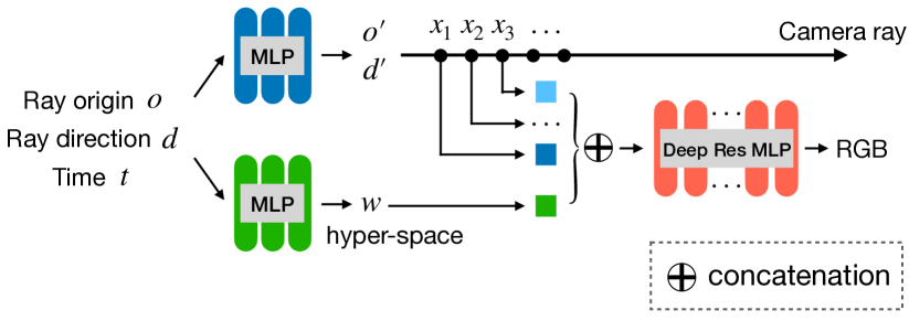
Figure 2: Schematic diagram of our proposed DyLiN architecture. We take a ray $r=(o,d)$ and time $t$ as input. We deform $r$ into $r^{\prime}=(o^{\prime},d^{\prime})$, and sample few points $x_{k}$, $k=1,\dots,K$ along $r^{\prime}$ to encode it (blue). In parallel, we also lift $r$ and $t$ to the hyperspace code $w$ (green), and concatenate it with each $x_{k}$. We use the concatenation to regress the RGB color of $r$ at $t$ directly (red).

Specifically, our deformation MLP $T_{\omega}$ maps an input ray $r=(o,d)$ to canonical space ray $r^{\prime}=(o^{\prime},d^{\prime})$:

$$(o^{\prime},d^{\prime})=T_{\omega}(o,d,t).$$ (1)

Unlike the pointwise deformation MLP proposed in Nerfies [27], which bends rays by offsetting their points independently, our MLP outputs rays explicitly, hence no ray bending occurs. Furthermore, after obtaining $r^{\prime}$, we encode it by sampling and concatenating $K$ points along it.

Our hyperspace MLP $H_{\psi}$ is similar to $T_{\omega}$, except it outputs a hyperspace representation $w$:

$$w=H_{\psi}(o,d,t).$$ (2)

In contrast to HyperNeRF [28], which predicts a hyperspace code $w$ for each 3D point, we use rays and compute a single $w$ for each ray.

Both MLPs further take the index $t$ as input to encode temporal deformations.

Once the $K$ points and $w$ are obtained, we concatenate them and feed the result into our LFN $R_{\pi}$, which is a deep residual color MLP regressor. Overall, we can collect the model parameters as $\phi=[\omega,\psi,\pi]$.

Note that without our two MLPs $T_{\omega}$ and $H_{\psi}$, our DyLiN falls back to the vanilla LFN.

3.1.2 Training Procedure

Our training procedure is composed of 3 phases.

First, we pretrain a dynamic NeRF model $F_{\theta}$ (e.g., D-NeRF [29] or HyperNeRF [28]) by randomly sampling time $t$ and input ray $r$, and minimizing the Mean Squared Error (MSE) against the corresponding RGB color of monocular target video $I$:

$$\min_{\theta}\,\mathbb{E}_{t,r=(o,d)}\left[\|F_{\theta}(o,d,t)-I(o,d,t)\|_{2}^{2}\right].$$ (3)

Recall, that $F_{\theta}$ is slow, as it performs numerical integration across the ray $r=(o,d)$.

Second, we employ the newly obtained $F_{\theta^{*}}$ as the teacher model for our DyLiN student model $G_{\phi}$ via KD. Specifically, we minimize the MSE loss against the respective pseudo ground truth ray color generated by $F_{\theta^{*}}$ across $S$ ray samples:

$$\min_{\phi}\,\mathbb{E}_{t,r=(o,d)}\left[\|G_{\phi}(o,d,t)-F_{\theta^{*}}(o,d,t)\|_{2}^{2}\right],$$ (4)

yielding $G_{\tilde{\phi}}$. Note how this is considerably different from R2L [36], which uses a static LFN that is distilled from a static NeRF.

Finally, we initialize our student model $G_{\phi}$ with parameters $\tilde{\phi}$ and fine-tune it using the original real video data:

$$\min_{\phi,\,\phi_{0}=\tilde{\phi}}\,\mathbb{E}_{t,r=(o,d)}\left[\|G_{\phi}(o,d,t)-I(o,d,t)\|_{2}^{2}\right],$$ (5)

obtaining $\phi^{*}$.

3.2 CoDyLiN

3.2.1 Network Architecture

We further demonstrate that our DyLiN architecture from Sec. 3.1.1 can be extended to the controllable scenario using attribute inputs with hyperspace MLPs and attention masks. Our proposed CoDyLiN network $Q_{\tau}$ is depicted in Fig. 3.

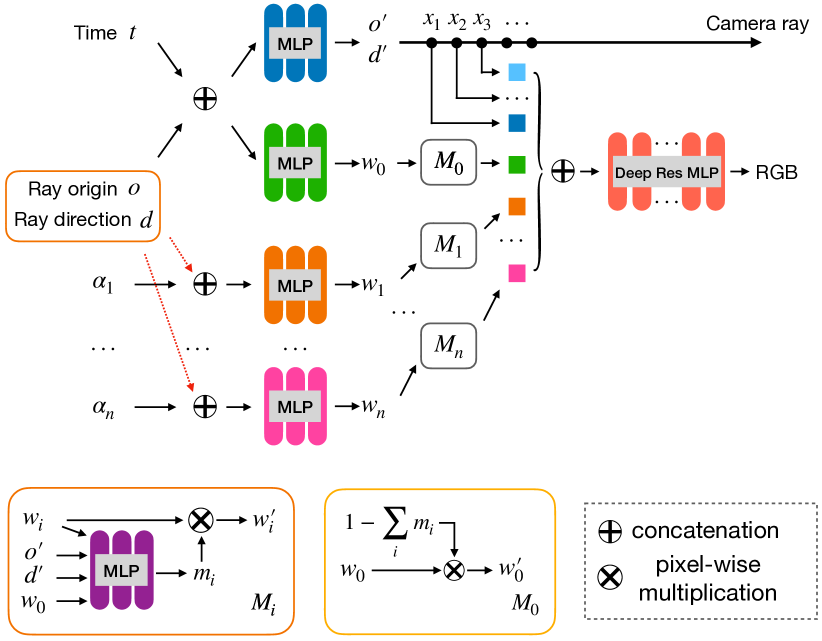
Figure 3: Schematic diagram of our proposed CoDyLiN architecture. We augment our DyLiN (blue, green, red) by introducing scalar attribute inputs $\alpha_{i}\in[-1,1]$, $i=1,\dots,n$ and lifting them to their respective hyperspace codes $w_{i}$ (orange, …, pink MLPs). Next, $M_{i}$ disentangles $w_{i}$ from $w_{j}$, $j\neq i$ by masking it into $w_{i}^{\prime}$ (orange, …, pink boxes and bottom insets). We concatenate the sampled points $x_{k}$, $k=1,\dots,K$ with the $w_{i}^{\prime}$, $i=1,\dots,n$ and predict the RGB color corresponding to the inputs (red). Arrows from $(o^{\prime},d^{\prime})$ and $w_{0}$ to $M_{i}$ are omitted from the top figure for simplicity. Compare this with Fig. 2.

Specifically, we start from DyLiN $G_{\phi}$ and add scalar inputs $\alpha_{i}\in[-1,1]$, $i=1,\dots,n$ next to $o,d,t$. Intuitively, these are given strength values for specific local attributes, which can be interpolated continuously. $n$ is the total number of attributes.

Each $\alpha_{i}$ is then processed independently with its own hyperspace MLP $H_{i,\psi_{i}}$ to yield the hyperspace code $w_{i}$:

$$w_{i}=H_{i,\psi_{i}}(o,d,t).$$ (6)

Next, we include mask MLP regressors $M_{i,\rho_{i}}$ to generate scalar attention masks $\hat{m}_{i}\in[0,1]$ for each $w_{i}$ (including $w_{0}=w$):

$$\hat{m}_{i} =M_{i,\rho_{i}}(w_{i},w,o,d),$$ (7)

$$\hat{m}_{0} =1-\sum_{i=1}^{n}{\hat{m}_{i}},$$

$$w_{i}^{\prime} =\hat{m}_{i}\cdot w_{i},\quad i=0,\dots,n,$$

This helps the architecture to spatially disentangle (i.e., localize) the effects of attributes $\alpha_{i}$, while $\hat{m}_{0}$ can be understood as the space not affected by any attributes.

Finally, we sample $K$ points on the ray similarly to Sec. 3.1.1, concatenate those with the $w_{i}^{\prime}$ vectors, and process the result further with LFN $R_{\pi}$. Again, we can use a shorthand for the parameters: $\tau=[\omega,\psi,\psi_{1},\dots,\psi_{n},\rho_{1},\dots,\rho_{n},\pi]$.

Observe that without our MLPs $H_{i,\psi_{i}}$, $M_{i,\rho_{i}}$, $i=1,\dots,n$, our CoDyLiN reverts to our simpler DyLiN. Different from CoNeRF [13], we process rays instead of points, and use the $\alpha_{i}$ as inputs instead of targets.

3.2.2 Training Procedure

Akin to Sec. 3.1.2, we split training into pretraining and distillation steps, but omit fine-tuning.

First, we pretrain a CoNeRF model $E_{\nu}$ [13] by randomly sampling $(t,r,i)$, against 3 ground truths: ray color, attribute values $\alpha_{i}$ and 2D per-attribute masks $m_{2D,i}$. This yields us $E_{\nu^{*}}$. For brevity, we omit the details of this step, and kindly forward the reader to Section 3 in [13].

Second, we distill from our teacher CoNeRF model $E_{\nu^{*}}$ into our student CoDyLiN $Q_{\tau}$ by randomly sampling $t,r,\alpha_{1},\dots,\alpha_{n}$, and minimizing the MSE against 2 pseudo ground truths, i.e., ray colors and 2D masks $\bar{m}_{2D,i}$:

$$\min_{\tau}\,\mathbb{E}_{t,r=(o,d)}\biggl{[}\|Q_{\tau}(o,d,t,\alpha_{1:n})-\bar{E}_{\nu^{*}}(o,d,t,\alpha_{1:n})\|_{2}^{2}\\ +\lambda_{m}\cdot\sum_{i=0}^{n}{\|\hat{m}_{i}(o,d,t,\alpha_{i})-\bar{m}_{2D}(o,d,t,\alpha_{1:n})_{i}\|_{2}^{2}}\biggr{]},$$ (8)

where $\bar{E}_{\nu}$ is identical to $E_{\nu}$ except for taking $\alpha_{1:n}=[\alpha_{1},\dots,\alpha_{n}]$ as input and outputting the masks $\bar{m}_{2D,i}$, $i=0,\dots,n$. We denote the result of the optimization as $Q_{\tau^{*}}$.

We highlight that our teacher and student models are both controllable in this setup.

4 Experimental Setup

4.1 Datasets

To test our hypotheses, we performed experiments on three types of dynamic scenes: synthetic, real and real controllable.
Synthetic Scenes. We utilized the synthetic $360^{\circ}$ dynamic dataset introduced by [29], which contains 8 animated objects with complicated geometry and realistic non-Lambertian materials. Each dynamic scene consists of $50$ to $200$ training images and $20$ testing images. We used $400\times 400$ image resolution. We applied D-NeRF [29] as our teacher model with the publicly available pretrained weights.
Real Scenes. We collected real dynamic data from $2$ sources. First, we utilized 5 topologically varying scenes provided by [28] (Broom, 3D Printer, Chicken, Americano and Banana), which were captured by a rig encompassing a pole with two Google Pixel 3 phones rigidly attached roughly $16\text{\,}\mathrm{cm}$ apart. Second, we collected human facial videos using an iPhone 13 Pro camera. We rendered both sets at $960\times 540$ image resolution. We pretrained a HyperNeRF [28] teacher model from scratch for each scene.
Real Controllable Scenes. We borrowed 2 real controllable scenes from [13] (closing/opening eyes/mouth, and transformer), which are captured either with a Google Pixel 3a or an Apple iPhone 13 Pro, and contain annotations over various attributes. We applied image resolution of $480\times 270$ pixels. We pretrained a CoNeRF [13] teacher model from scratch per scene.

4.2 Settings

Throughout our experiments, we use the settings listed below, many of which follow [36].

In order to retain efficiency, we define $T_{\omega}$ and $H_{\psi}$ to be small MLPs, with $T_{\omega}$ consisting of $7$ layers of $128$ units with $r^{\prime}\in\mathbb{R}^{6}$, and $H_{\psi}$ having $6$ layers of $64$ units with $w\in\mathbb{R}^{8}$. Then, we use $K=16$ sampled points to represent rays, where sampling is done randomly during training and evenly spaced during inference.

Contrary to $T_{\omega}$ and $H_{\psi}$, our LFN $R_{\pi}$ is a very deep residual color MLP regressor, containing $88$ layers with $256$ units per layer, in order to have enough capacity to learn the video generation process.

We generate rays within Eqs. 3, 4, 5 and 8 by sampling ray origins $o=(x_{o},y_{o},z_{o})$ and normalized directions $d=(x_{d},y_{d},z_{d})$ randomly from the uniform distribution $U$ as follows:

$$x_{o} \sim U(x_{o}^{min},x_{o}^{max}),\quad x_{d} \sim U(x_{d}^{min},x_{d}^{max}),$$ (9)

$$y_{o} \sim U(y_{o}^{min},y_{o}^{max}),\quad y_{d} \sim U(y_{d}^{min},y_{d}^{max}),$$ (10)

$$z_{o} \sim U(z_{o}^{min},z_{o}^{max}),\quad z_{d} \sim U(z_{d}^{min},z_{d}^{max}),$$ (11)

where the $min,max$ bounds of the 6 intervals are inferred from the original training video. In addition to uniform sampling, we also apply the hard example mining strategy suggested in [36] to focus on fine-grained details. We used $S=$10,000\text{\,}$$ training samples during KD in (4).

Subsequently, we also randomly sample time step $t$ uniformly from the unit interval: $t\sim U(0,1)$.

Optionally, for our CoDyLiN experiments, we define each $H_{i,\psi_{i}}$ to be a small MLP having $5$ layers of $128$ units with $w_{i}\in\mathbb{R}^{8}$. During training, we uniformly sample attributes within $[-1,1]$: $\alpha_{i}\sim U(-1,1)$, and let $\lambda_{m}=0.1$.

During training, we used Adam [14] with learning rate $5\text{\times}{10}^{-4}\text{\,}$ and batch size $4,096\text{\,}$.

We performed all experiments on single NVIDIA A100 GPUs.

4.3 Baseline Models

For testing our methods, we compared quality and speed against several baseline models, including NeRF [23], NV [19], NSFF [16], Nerfies [27], HyperNeRF [28], two variants of TiNeuVox [8], DirectVoxGo [33], Plenoxels [9], T-NeRF and D-NeRF [29], as well as CoNeRF [13].

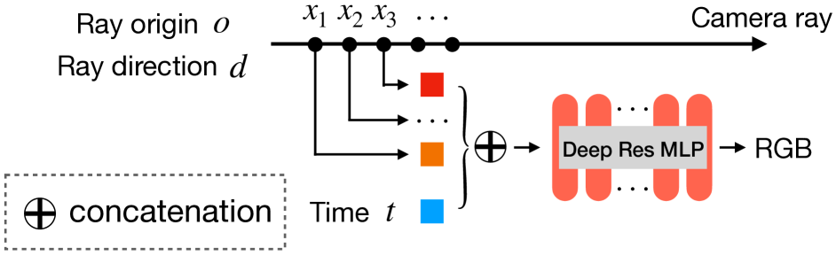
(a)

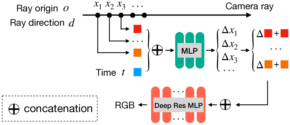
(b)

Figure 4: Our two ablated baseline models, omiting components of our DyLiN. (a) Without our two proposed MLPs. (b) Pointwise deformation MLP only, predicting offsets jointly.

In addition, we performed an ablation study by comparing against 2 simplified versions of our DyLiN architecture. First, we omitted both of our deformation and hyperspace MLPs and simply concatenated the time step $t$ to the sampled ray points (essentially resulting in a dynamic R2L). This method is illustrated in Fig. 4(a). Second, we employed a pointwise deformation MLP ($5$ layers of $256$ units) inspired by [29], which deforms points along a ray by predicting their offsets jointly, i.e., it can bend rays. This is contrast to our DyLiN, which deforms rays explicitly without bending and also applies a hyperspace MLP. This scheme is depicted in Fig. 4(b). In both baselines, the deep residual color MLP regressors were kept intact. Next, we also tested the effects of our fine-tuning procedure from (5) by training all of our models both with and without it. Lastly, we assessed the dependences on the number of sampled points along rays $K$ and on the number of training samples $S$ during KD in (4).

4.4 Evaluation Metrics

For quantitatively evaluating the quality of generated images, we calculated the Peak Signal-to-Noise Ratio (PSNR) [12] in decibels ($\mathrm{dB}$), the Structural Similarity Index (SSIM) [40, 25], the Multi-Scale SSIM (MS-SSIM) [41] and the Learned Perceptual Image Patch Similarity (LPIPS) [44] metrics. Intuitively, PSNR is a pixelwise score, while SSIM and MS-SSIM also take pixel correlations and multiple scales into account, respectively, yet all of these tend to favor blurred images. LPIPS compares deep neural representations of images and is much closer to human perception, promoting semantically better and sharper images.

Furthermore, for testing space and time complexity, we computed the storage size of parameters in megabytes (MB) and measured the wall-clock time in milliseconds (ms) while rendering the synthetic Lego scene with each model.

5 Results

5.1 Quantitative Results

Tab. 1 and Tab. 2 contain our quantitative results for reconstruction quality on synthetic and real dynamic scenes, accordingly. We found that among prior works, TiNeuVox-B performed the best on synthetic scenes with respect to each metric. On real scenes, however, NSFF took the lead. Despite having strong metrics, NSFF is qualitatively poor and slow. Surprisingly, during ablation, even our most basic model (DyLiN without the two MLPs from Fig. 4(a)) could generate perceptually better looking images than TiNeuVox-B, thanks to the increased training dataset size via KD. Incorporating the MLPs $T_{\omega}$ and $H_{\psi}$ into the model each improved results slightly. Interestingly, fine-tuning on real data as in (5) gave a substantial boost. In addition, our relative PSNR improvement over the teacher model (Tab. 1=$+$1.93\text{\,}\mathrm{dB}$$, up to $+$3.16\text{\,}\mathrm{dB}$$ per scene; Tab. 2=$+$2.7\text{\,}\mathrm{dB}$$, up to $+$13.14\text{\,}\mathrm{dB}$$) is better than that of R2L [36] ($+$1.4\text{\,}\mathrm{dB}$$, up to $+$2.8\text{\,}\mathrm{dB}$$).

Table 1: Quantitative results on synthetic dynamic scenes. Notations: Multi-Layer Perceptron (MLP), PD (pointwise deformation), FT (fine-tuning). We utilized D-NeRF as the teacher model for our DyLiNs. The winning numbers are highlighted in bold.

Method	PSNR$\uparrow$	SSIM$\uparrow$	LPIPS$\downarrow$
NeRF[23]	19.00	0.8700	0.1825
DirectVoxGo[33]	18.61	0.8538	0.1688
Plenoxels[9]	20.24	0.8688	0.1600
T-NeRF[29]	29.51	0.9513	0.0788
D-NeRF[29]	30.50	0.9525	0.0663
TiNeuVox-S[8]	30.75	0.9550	0.0663
TiNeuVox-B[8]	32.67	0.9725	0.0425
DyLiN, w/o two MLPs, w/o FT (ours)	31.16	0.9931	0.0281
DyLiN, w/o two MLPs (ours)	32.07	0.9937	0.0196
DyLiN, PD MLP only, w/o FT (ours)	31.26	0.9932	0.0279
DyLiN, PD MLP only (ours)	31.24	0.9940	0.0189
DyLiN, w/o FT (ours)	31.37	0.9933	0.0275
DyLiN (ours)	32.43	0.9943	0.0184

Table 2: Quantitative results on real dynamic scenes. Notations: Multi-Layer Perceptron (MLP), PD (pointwise deformation), FT (fine-tuning). We utilized HyperNeRF as the teacher model for our DyLiNs. The winning numbers are highlighted in bold.

Method	PSNR$\uparrow$	MS-SSIM$\uparrow$
NeRF[23]	20.1	0.745
NV[19]	16.9	0.571
NSFF[16]	26.3	0.916
Nerfies[27]	22.2	0.803
HyperNeRF[28]	22.4	0.814
TiNeuVox-S[8]	23.4	0.813
TiNeuVox-B[8]	24.3	0.837
DyLiN, w/o two MLPs, w/o FT (ours)	23.8	0.882
DyLiN, w/o two MLPs (ours)	24.2	0.894
DyLiN, PD MLP only, w/o FT (ours)	23.9	0.885
DyLiN, PD MLP only (ours)	24.6	0.903
DyLiN, w/o FT (ours)	24.0	0.886
DyLiN (ours)	25.1	0.910

Table 3: Quantitative results for space and time complexity on the synthetic Lego scene. Notations: Multi-Layer Perceptron (MLP), PD (pointwise deformation), FT (fine-tuning).

	Storage	Wall-clock
Method	(MB)	time (ms)
NeRF[23]	005.00	2,950.0
DirectVoxGo[33]	205.00	1,090.0
Plenoxels[9]	717.00	0,050.0
NV[19]	439.00	0,074.9
D-NeRF[29]	004.00	8,150.0
NSFF[16]	014.17	5,450.0
HyperNeRF[28]	015.36	2,900.0
TiNeuVox-S[8]	023.70	3,280.0
TiNeuVox-B[8]	023.70	6,920.0
DyLiN, w/o two MLPs, w/o FT (ours)	068.04	0,115.4
DyLiN, w/o two MLPs (ours)	068.04	0,115.4
DyLiN, PD MLP only, w/o FT (ours)	072.60	0,115.7
DyLiN, PD MLP only (ours)	072.60	0,115.7
DyLiN, w/o FT (ours)	070.11	0,116.0
DyLiN (ours)	070.11	0,116.0

Tab. 3 shows quantitative results for space and time complexity on the synthetic Lego scene. We found that there is a trade-off between the two metrics, as prior works are typically optimized for just one of those. In contrast, all of our proposed DyLiN variants settle at the golden mean between the two extremes. When compared to the strongest baseline TiNeuVox-B, our method requires $3$ times as much storage but is nearly 2 orders of magnitude faster. Plenoxels and NV, the only methods that require less computation than ours, perform much worse in quality.

Fig. 5 reports quantitative ablation results for dependencies on the number of sampled points per ray $K$ and on the number of training samples during KD $S$, performed on the synthetic Standup scene. For dependence on $K$ (Fig. 5(a)), we found that there were no significant differences between test set PNSR scores for $K\in\{4,8,16,32\}$, while we encountered overfitting for $K\in\{64,128\}$. This justified our choice of $K=16$ for the rest of our experiments. Regarding the effect of $S$ (Fig. 5(b)), overfitting occured for smaller sample sizes including $S\in\{100;500;$1,000\text{\,}$;$5,000\text{\,}\}$$. The test and training set PSNR scores were much closer for $S=$10,000\text{\,}$$, validating our general setting.

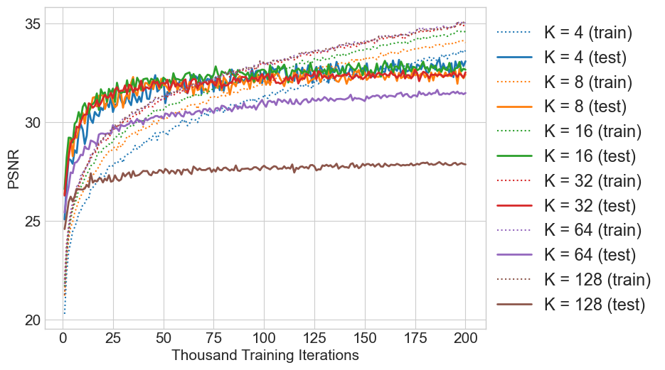
(a)

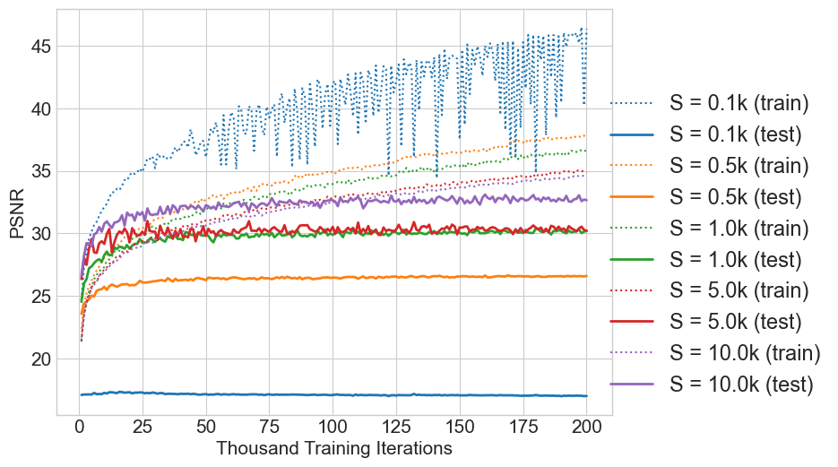
(b)

Figure 5: Quantitative results for ablation on the synthetic Standup scene. (a) Dependence on the number of sampled points $K$ across ray $r^{\prime}$. (b) Dependence on the number of training samples $S$ during Knowledge Distillation (KD).

Our controllable numerical results are collected in Tab. 4. In short, our CoDyLiN was able to considerably outperform CoNeRF with respect to MS-SSIM and speed.

Table 4: Quantitative results on real controllable scenes. We utilized CoNeRF as the teacher model for our CoDyLiN. The winning numbers are highlighted in bold.

	Eyes/Mouth			Transformer
			Wall-clock			Wall-clock
Method	PSNR$\uparrow$	MS-SSIM$\uparrow$	time ($\mathrm{ms}$)	PSNR$\uparrow$	MS-SSIM$\uparrow$	time ($\mathrm{ms}$)
CoNeRF[13]	21.4658	0.7458	6230.0	23.0319	0.8878	4360.0
CoDyLiN (ours)	21.4655	0.9510	0116.3	23.5882	0.9779	0116.0

5.2 Qualitative Results

Fig. 6 and Fig. 7 depict qualitative results for reconstruction quality on synthetic and real dynamic scenes, respectively. Both show that our full DyLiN model generated the sharpest, most detailed images, as it was able to capture cloth wrinkles (Fig. 6(j)) and the eye of the chicken (Fig. 7(e)). The competing methods tended to oversmooth these features. We also ablated the effect of omitting fine-tuning (Fig. 6(i), Fig. 7(d)), and results declined considerably.

For the sake of completeness, Fig. 8 illustrates qualitative ablation results for our model components on real dynamic scenes. We found that sequentially adding our two proposed MLPs $T_{\omega}$ and $H_{\psi}$ improves the reconstruction, e.g., the gum between the teeth (Fig. 8(e)) and the fingers (Fig. 8(j)) become more and more apparent. Without the MLPs, these parts were heavily blurred (Fig. 8(c), Fig. 8(h)).

We kindly ask readers to refer to the supplementary material for CoDyLiN’s qualitative results.

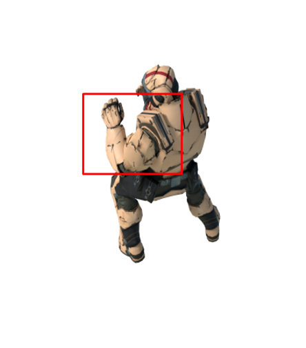
Hook

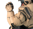
(a) Ground Truth

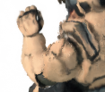
(b) D-NeRF [29]

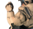
(c) TiNeuVox [8]

(d) Ours-1

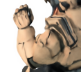
(e) Ours-2

Jumping Jacks

(f) Ground Truth

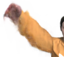
(g) D-NeRF [29]

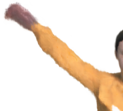
(h) TiNeuVox [8]

(i) Ours-1

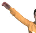
(j) Ours-2

Figure 6: Qualitative results on synthetic dynamic scenes. We compare our DyLiN (Ours-1, Ours-2) with the ground truth, the D-NeRF teacher model and TiNeuVox. Ours-1 and Ours-2 were trained without and with fine-tuning on the original data, respectively.

Chicken

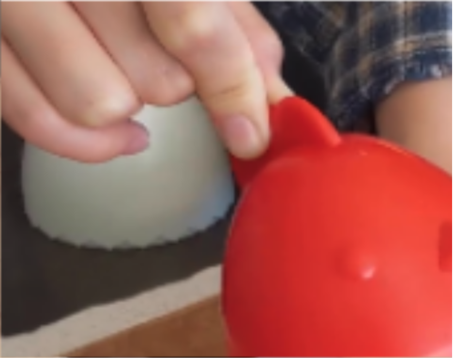
(a) Ground Truth

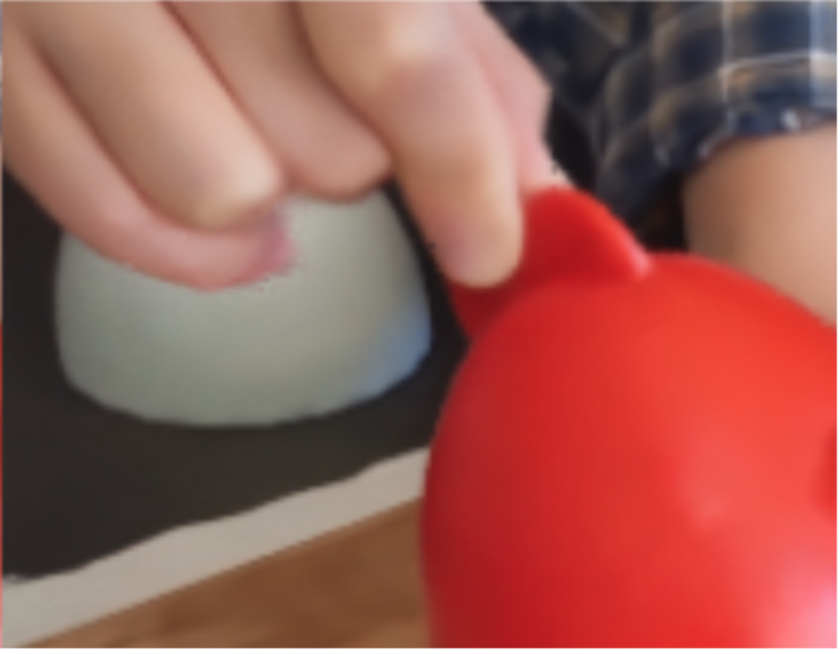
(b) HyperNeRF [28]

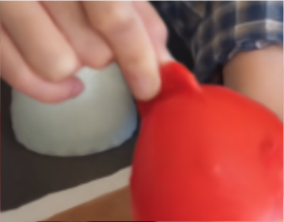
(c) TiNeuVox [8]

(d) Ours-1

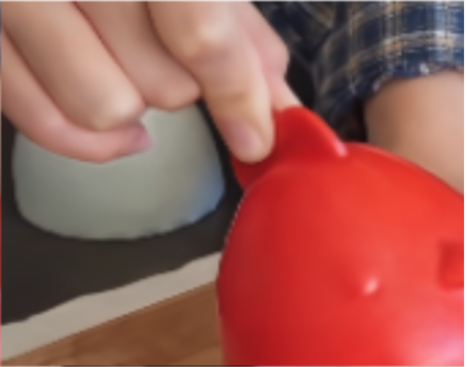
(e) Ours-2

Figure 7: Qualitative results on a real dynamic scene. We compare our DyLiN (Ours-1, Ours-2) with the ground truth, the HyperNeRF teacher model and TiNeuVox. Ours-1 and Ours-2 were trained without and with fine-tuning on the original data, respectively.

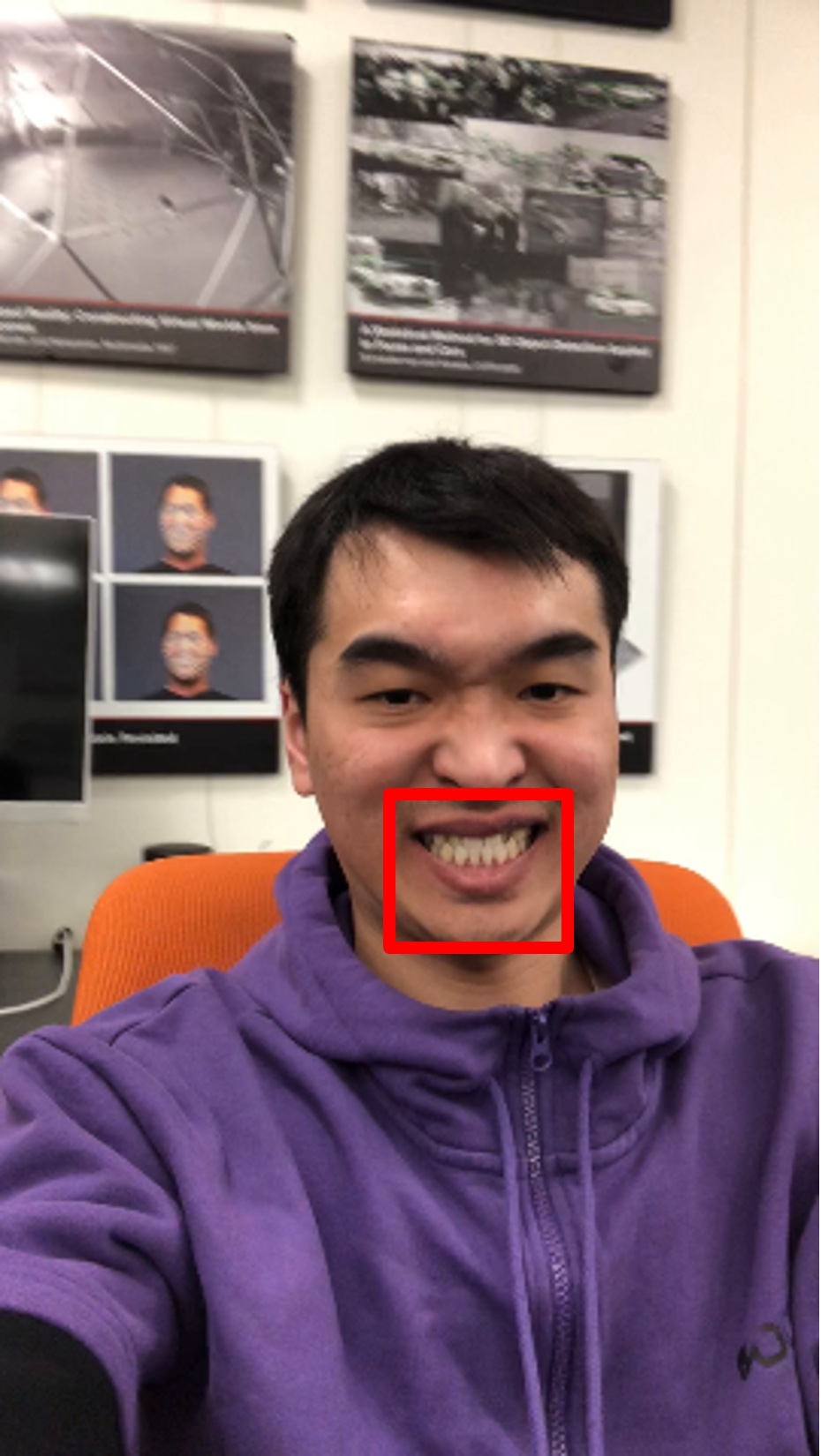
Expression

(a) Ground Truth

(b) HyperNeRF [28]

(c) Ours-1

(d) Ours-2

(e) Ours-3

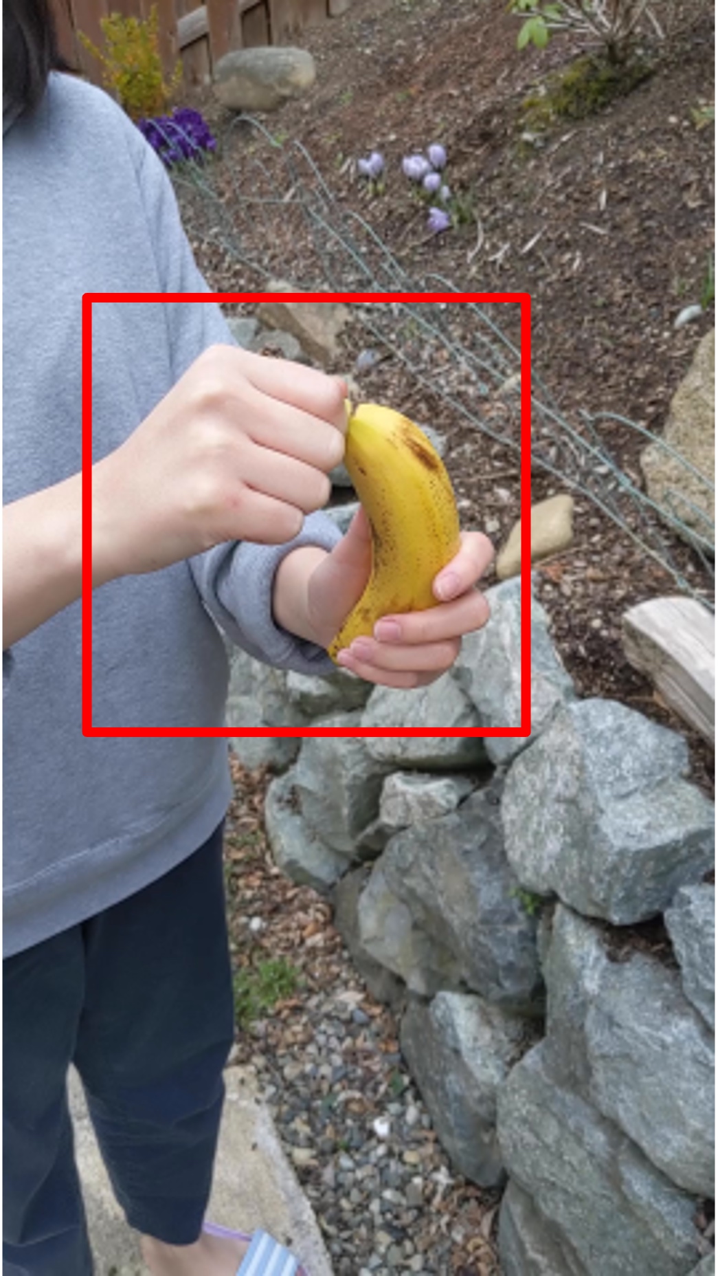
Peel Banana

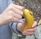
(f) Ground Truth

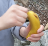
(g) HyperNeRF [28]

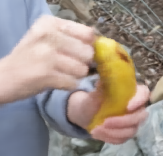
(h) Ours-1

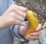
(i) Ours-2

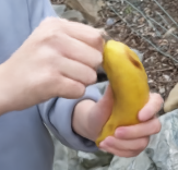
(j) Ours-3

Figure 8: Qualitative results for ablation on real dynamic scenes. We compare our DyLiN (Ours-1, Ours-2, Ours-3) with the ground truth and the HyperNeRF teacher model. Ours-1 was trained without our two MLPs. Ours-2 was trained with pointwise deformation MLP only. Ours-3 is our full model with both of our proposed two MLPs.

6 Conclusion

We proposed two architectures for extending LFNs to dynamic scenes. Specifically, we introduced DyLiN, which models ray deformations without bending and lifts whole rays into a hyperspace, and CoDyLiN, which allows for controllable attribute inputs. We trained both techniques via knowledge distillation from various dynamic NeRF teacher models. We found that DyLiN produces state-of-the-art quality even without ray bending and CoDyLiN outperforms its teacher model, while both are nearly 2 orders of magnitude faster than their strongest baselines.

Our methods do not come without limitations, however. Most importantly, they focus on speeding up inference, as they require pretrained teacher models, which can be expensive to obtain. In some experiments, our solutions were outperformed in terms of the PSNR score. Using the winners as teacher models could improve performance. Additionally, distillation from multiple teacher models or joint training of the teacher and student models are also yet to be explored. Moreover, we currently represent rays implicitly by sampling $K$ points along them, but increasing this number can lead to overfitting. An explicit ray representation may be more effective. Finally, voxelizing and quantizing our models could improve efficiency.

Our results are encouraging steps towards achieving real-time volumetric rendering and animation, and we hope that our work will contribute to the progress in these areas.

References

- [1] E.H. Adelson and J.Y.A. Wang. Single Lens Stereo with a Plenoptic Camera. IEEE Trans. Pattern Anal. Mach. Intell., 14(2):99–106, 1992.
- [2] Jonathan T Barron, Ben Mildenhall, Matthew Tancik, Peter Hedman, Ricardo Martin-Brualla, et al. Mip-NeRF: A Multiscale Representation for Anti-Aliasing Neural Radiance Fields. In Proc. IEEE/CVF ICCV, pages 5855–5864, 2021.
- [3] James R Bergen and Edward H Adelson. The Plenoptic Function and the Elements of Early Vision. Comput. Model. Vis. Process., 1:8, 1991.
- [4] Cristian Buciluǎ, Rich Caruana, and Alexandru Niculescu-Mizil. Model Compression. In Proc. 12th ACM SIGKDD ICKDDM, pages 535–541, 2006.
- [5] Guobin Chen, Wongun Choi, Xiang Yu, Tony Han, and Manmohan Chandraker. Learning Efficient Object Detection Models with Knowledge Distillation. Adv. NeurIPS, 30, 2017.
- [6] Zhiqin Chen. IM-NET: Learning implicit fields for generative shape modeling. PhD thesis, Applied Sciences: School of Computing Science, 2019.
- [7] Kangle Deng, Andrew Liu, Jun-Yan Zhu, and Deva Ramanan. Depth-supervised NeRF: Fewer Views and Faster Training for Free. In Proc. IEEE/CVF CVPR, pages 12882–12891, 2022.
- [8] Jiemin Fang, Taoran Yi, Xinggang Wang, Lingxi Xie, Xiaopeng Zhang, et al. Fast Dynamic Radiance Fields with Time-Aware Neural Voxels. arXiv:2205.15285, 2022.
- [9] Sara Fridovich-Keil, Alex Yu, Matthew Tancik, Qinhong Chen, Benjamin Recht, et al. Plenoxels: Radiance Fields Without Neural Networks. In Proc. IEEE/CVF CVPR, pages 5501–5510, 2022.
- [10] Guy Gafni, Justus Thies, Michael Zollhofer, and Matthias Nießner. Dynamic Neural Radiance Fields for Monocular 4D Facial Avatar Reconstruction. In Proc. IEEE/CVF CVPR, pages 8649–8658, 2021.
- [11] Steven J Gortler, Radek Grzeszczuk, Richard Szeliski, and Michael F Cohen. The Lumigraph. In Proc. 23rd CGIT, pages 43–54, 1996.
- [12] Alain Hore and Djemel Ziou. Image quality metrics: PSNR vs. SSIM. In 20th ICPR, pages 2366–2369. IEEE, 2010.
- [13] Kacper Kania, Kwang Moo Yi, Marek Kowalski, Tomasz Trzciński, and Andrea Tagliasacchi. CoNeRF: Controllable Neural Radiance Fields. In Proc. IEEE/CVF CVPR, pages 18623–18632, 2022.
- [14] Diederik P Kingma and Jimmy Ba. Adam: A Method for Stochastic Optimization. arXiv:1412.6980, 2014.
- [15] Marc Levoy and Pat Hanrahan. Light Field Rendering. In Proc. 23rd CGIT, pages 31–42, 1996.
- [16] Zhengqi Li, Simon Niklaus, Noah Snavely, and Oliver Wang. Neural Scene Flow Fields for Space-Time View Synthesis of Dynamic Scenes. In Proc. IEEE/CVF CVPR, 2021.
- [17] David B Lindell, Julien NP Martel, and Gordon Wetzstein. AutoInt: Anutomatic Integration for Fast Neural Volume Rendering. In Proc. IEEE/CVF CVPR, pages 14556–14565, 2021.
- [18] Lingjie Liu, Jiatao Gu, Kyaw Zaw Lin, Tat-Seng Chua, and Christian Theobalt. Neural Sparse Voxel Fields. Adv. NeurIPS, 33:15651–15663, 2020.
- [19] Stephen Lombardi, Tomas Simon, Jason Saragih, Gabriel Schwartz, Andreas Lehrmann, et al. Neural Volumes: Learning Dynamic Renderable Volumes from Images. ACM Trans. Graph., 38(4):65:1–65:14, July 2019.
- [20] Ricardo Martin-Brualla, Noha Radwan, Mehdi SM Sajjadi, Jonathan T Barron, Alexey Dosovitskiy, et al. NeRF in the Wild: Neural Radiance Fields for Unconstrained Photo Collections. In Proc. IEEE/CVF CVPR, pages 7210–7219, 2021.
- [21] Lars Mescheder, Michael Oechsle, Michael Niemeyer, Sebastian Nowozin, and Andreas Geiger. Occupancy Networks: Learning 3D Reconstruction in Function Space. In Proc. IEEE/CVF CVPR, pages 4460–4470, 2019.
- [22] Ben Mildenhall, Peter Hedman, Ricardo Martin-Brualla, Pratul P Srinivasan, and Jonathan T Barron. NeRF in the Dark: High Dynamic Range View Synthesis from Noisy Raw Images. In Proc. IEEE/CVF CVPR, pages 16190–16199, 2022.
- [23] Ben Mildenhall, Pratul P Srinivasan, Matthew Tancik, Jonathan T Barron, Ravi Ramamoorthi, et al. NeRF: Representing Scenes as Neural Radiance Fields for View Synthesis. Commun. ACM, 65(1):99–106, 2021.
- [24] Thomas Neff, Pascal Stadlbauer, Mathias Parger, Andreas Kurz, Joerg H Mueller, et al. Donerf: Towards real-time rendering of compact neural radiance fields using depth oracle networks. In CGF, volume 40, pages 45–59. Wiley Online Library, 2021.
- [25] Augustus Odena, Christopher Olah, and Jonathon Shlens. Conditional Image Synthesis with Auxiliary Classifier GANs. In ICML, pages 2642–2651. PMLR, 2017.
- [26] Jeong Joon Park, Peter Florence, Julian Straub, Richard Newcombe, and Steven Lovegrove. DeepSDF: Learning Continuous Signed Distance Functions for Shape Representation. In Proc. IEEE/CVF CVPR, pages 165–174, 2019.
- [27] Keunhong Park, Utkarsh Sinha, Jonathan T Barron, Sofien Bouaziz, Dan B Goldman, et al. Nerfies: Deformable Neural Radiance Fields. In Proc. IEEE/CVF ICCV, pages 5865–5874, 2021.
- [28] Keunhong Park, Utkarsh Sinha, Peter Hedman, Jonathan T Barron, Sofien Bouaziz, et al. HyperNeRF: A Higher-Dimensional Representation for Topologically Varying Neural Radiance Fields. ACM Trans. Graph., 40(6):1–12, 2021.
- [29] Albert Pumarola, Enric Corona, Gerard Pons-Moll, and Francesc Moreno-Noguer. D-NeRF: Neural Radiance Fields for Dynamic Scenes. In Proc. IEEE/CVF CVPR, pages 10318–10327, 2021.
- [30] Daniel Rebain, Wei Jiang, Soroosh Yazdani, Ke Li, Kwang Moo Yi, et al. DeRF: Decomposed Radiance Fields. In Proc. IEEE/CVF CVPR, pages 14153–14161, 2021.
- [31] Christian Reiser, Songyou Peng, Yiyi Liao, and Andreas Geiger. KiloNeRF: Speeding up Neural Radiance Fields with Thousands of Tiny MLPs. In Proc. IEEE/CVF ICCV, pages 14335–14345, 2021.
- [32] Vincent Sitzmann, Semon Rezchikov, William T. Freeman, Joshua B. Tenenbaum, and Fredo Durand. Light Field Networks: Neural Scene Representations with Single-Evaluation Rendering. In Proc. NeurIPS, 2021.
- [33] Cheng Sun, Min Sun, and Hwann-Tzong Chen. Direct Voxel Grid Optimization: Super-fast Convergence for Radiance Fields Reconstruction. In Proc. IEEE/CVF CVPR, 2022.
- [34] Edgar Tretschk, Ayush Tewari, Vladislav Golyanik, Michael Zollhöfer, Christoph Lassner, et al. Non-Rigid Neural Radiance Fields: Reconstruction and Novel View Synthesis of a Dynamic Scene From Monocular Video. In Proc. IEEE/CVF ICCV, pages 12959–12970, 2021.
- [35] Huan Wang, Yijun Li, Yuehai Wang, Haoji Hu, and Ming-Hsuan Yang. Collaborative Distillation for Ultra-Resolution Universal Style Transfer. In Proc. IEEE/CVF CVPR, pages 1860–1869, 2020.
- [36] Huan Wang, Jian Ren, Zeng Huang, Kyle Olszewski, Menglei Chai, et al. R2L: Distilling Neural Radiance Field to Neural Light Field for Efficient Novel View Synthesis. arXiv:2203.17261, 2022.
- [37] Lin Wang and Kuk-Jin Yoon. Knowledge distillation and student-teacher learning for visual intelligence: A review and new outlooks. IEEE Trans. Pattern Anal. Mach. Intell., 2021.
- [38] Liao Wang, Jiakai Zhang, Xinhang Liu, Fuqiang Zhao, Yanshun Zhang, et al. Fourier PlenOctrees for Dynamic Radiance Field Rendering in Real-time. In Proc. IEEE/CVF CVPR, pages 13524–13534, 2022.
- [39] Peng Wang, Lingjie Liu, Yuan Liu, Christian Theobalt, Taku Komura, et al. NeuS: Learning Neural Implicit Surfaces by Volume Rendering for Multi-view Reconstruction. Adv. NeurIPS, 34:27171–27183, 2021.
- [40] Zhou Wang, Alan C Bovik, Hamid R Sheikh, and Eero P Simoncelli. Image Quality Assessment: From Error Visibility to Structural Similarity. IEEE Trans. Image Process., 13(4):600–612, 2004.
- [41] Zhou Wang, Eero P Simoncelli, and Alan C Bovik. Multiscale structural similarity for image quality assessment. In The 37th Asilomar SSC, volume 2, pages 1398–1402. Ieee, 2003.
- [42] Qiangeng Xu, Zexiang Xu, Julien Philip, Sai Bi, Zhixin Shu, et al. Point-NeRF: Point-based Neural Radiance Fields. In Proc. IEEE/CVF CVPR, pages 5438–5448, 2022.
- [43] Alex Yu, Ruilong Li, Matthew Tancik, Hao Li, Ren Ng, et al. PlenOctrees for Real-time Rendering of Neural Radiance Fields. In Proc. IEEE/CVF ICCV, pages 5752–5761, 2021.
- [44] Richard Zhang, Phillip Isola, Alexei A Efros, Eli Shechtman, and Oliver Wang. The Unreasonable Effectiveness of Deep Features as a Perceptual Metric. In Proc. IEEE/CVF CVPR, pages 586–595, 2018.