Variational Inference for Longitudinal Data Using Normalizing Flows

Abstract

This paper introduces a new latent variable generative model able to handle high dimensional longitudinal data and relying on variational inference. The time dependency between the observations of an input sequence is modelled using normalizing flows over the associated latent variables. The proposed method can be used to generate either fully synthetic longitudinal sequences or trajectories that are conditioned on several data in a sequence and demonstrates good robustness properties to missing data. We test the model on 6 datasets of different complexity and show that it can achieve better likelihood estimates than some competitors as well as more reliable missing data imputation.

1 Introduction

Longitudinal data are more than common in many application fields such a medicine e.g. for disease progression modelling  (Aghili et al., 2018; Zhao et al., 2021) or monitoring treatment response (Blackledge et al., 2014). They consist in the observation of a given entity’s or individual’s evolution though time but contrary to time-series, the number of observations of a single entity may be pretty small. Moreover, such data can be of high dimension (e.g. images) and we may only have access to a reduce number of different entities (e.g. rare diseases follow-ups) leading to small databases and missing values (e.g. a missing observation at a given time or loss in follow-up of a given entity). All of these aspects make these data challenging to model.

Generative models such as Variational Autoencoders (VAEs) introduced in (Kingma & Welling, 2014; Rezende et al., 2014) appeared to be powerful models to model distributions and would be an interesting choice to consider for longitudinal data. Unfortunately, while they appear to be able to perform some disentanglement of the input data in their latent space (Higgins et al., 2017; Burgess, 2018; Kim & Mnih, 2018; Chen et al., 2018b), they struggle to capture more complex correlations such as time evolution for longitudinal data (Ramchandran et al., 2021). To address this limitation and improve the latent representations of the input data, methods trying to account for the correlations of the data in the latent space of VAEs (Sohn et al., 2015), proposing new prior distributions (Nalisnick et al., 2016; Sønderby et al., 2016; Dilokthanakul et al., 2017; Tomczak & Welling, 2018; Razavi et al., 2020; Pang et al., 2020) or seeking to enhance the expressiveness of the approximate posterior distribution (Salimans et al., 2015; Rezende & Mohamed, 2015) were proposed. With a specific focus on temporal coherence, works introducing priors using Gaussian Processes were also introduced (Casale et al., 2018; Fortuin et al., 2020; Ramchandran et al., 2021). Nonetheless, those models were mainly designed to perform missing data imputation or for conditional settings and so are not well suited for unconditional sequence generation. Approaches relying on neural ODE (NODE) (Chen et al., 2018c; Xu et al., 2021; Massaroli et al., 2020; Dupont et al., 2019), deep state models (Rangapuram et al., 2018; Klushyn et al., 2021), latent RNN models (Chung et al., 2015; Serban et al., 2017) or latent SDE (Tzen & Raginsky, 2019; Li et al., 2020) have also demonstrated promising results to model time dependent data and to perform time series forecasting, interpolation or for classification purposes. Nonetheless, their applicability to the context of unconditional high dimensional data generation remains poorly explored.

Focusing more specifically on medical applications, several works have analysed longitudinal data through the prism of progression models using in particular mixed-effects models (Schiratti et al., 2015; Bône et al., 2018). In these approaches, patients are assumed to follow a given trajectory that deviates from a reference curve that may, for example, represent the average progression of a given disease. These approaches were then combined with dimensionality reduction using autoencoders (Louis et al., 2019) or VAEs (Sauty & Durrleman, 2022). However, these methods remain limited to the context of disease progression because they assume the existence of an intrinsic average trajectory from which each subject deviates, which may no longer be a valid assumption for heterogeneous datasets.

In this paper, we take quite a different approach and propose the following contributions:

• We propose a new generative latent variable model imposing time dependency of the observations in an input sequence using normalizing flows on the associated latent variables. A training procedure relying on variational inference is also derived.

• We show that the model is capable of handling high dimensional longitudinal data and able to generate fully synthetic sequences or trajectories conditioned on several input data.

• We discuss the modularity of the proposed model and show that it can benefit pretty easily from improvements available in the variational inference literature.

• We show that the method achieves better likelihood estimates that competitors on benchmark datasets and can outperform them for missing data imputation.

2 Background

In this section, we first recall some elements on variational inference and normalizing flows needed in the proposed method.

2.1 Variational Inference

Given observations $x\in\mathbb{R}^{D}$ and associated latent variables $z\in\mathbb{R}^{d}$ with joint distribution $p(x,z)$, variational inference (Jordan et al., 1999) is a method that aims at approximating an untractable conditional distribution $p(z|x)$ of the latent variables given the observations using a family of parametrized distributions $q_{\phi}(z|x)$ (Blei et al., 2017). The idea is to find the set of parameters $\phi$ that minimises the Kullback-Leibler (KL) divergence between the approximate posterior and the true one i.e. $\min\limits_{\phi}\mathrm{KL}(q_{\phi}(z|x)||p(z|x))$. However, this objective is most of the time untractable since $p(z|x)$ is unknown and so a surrogate objective is optimised instead and obtained using Jensen’s inequality (Jordan et al., 1999):

$$\log p(x)=\log\int_{\mathbb{R}^{d}}p(x,z)dz =\log\mathbb{E}_{q_{\phi}}\Bigg{[}\frac{p(x,z)}{q_{\phi}(z|x)}\Bigg{]}\geq\mathbb{E}_{q_{\phi}}\log\Bigg{[}\frac{p(x,z)}{q_{\phi}(z|x)}\Bigg{]}\,.$$ (1)

The right hand side of the equation is called the Evidence Lower BOund (ELBO) and one may notice that the difference between the left hand side of the equation and the ELBO gives $\mathrm{KL}(q_{\phi}(z|x)||p(z|x))$. Hence, maximising the ELBO amounts to minimising the KL and so the ELBO is used as objective for the variational approximation.

2.2 Normalizing Flows

Normalizing flows are flexible models that can be used to transform simple probability densities into much complex ones by re-coursing to sequences of invertible smooth mappings. They have, for instance, been proposed to enhance the expressiveness of the approximate posterior distribution used in the context of variational inference in (Rezende & Mohamed, 2015). These models rely on the rule of change of variables such that if $z\in\mathbb{R}^{d}$ is a random variable that follows the distribution $q(z)$ and $f:\mathbb{R}^{d}\to\mathbb{R}^{d}$ is an invertible smooth function, then the random variable $z^{\prime}=f(z)$ has a distribution given by

$$q(z^{\prime})=q(z)\bigg{|}\det\frac{\partial f^{-1}}{\partial z^{\prime}}\bigg{|}=q(z)\bigg{|}\det\frac{\partial f}{\partial z}\bigg{|}^{-1}\,.$$ (2)

In this setting, $f$ is called a normalizing flow and so several flows can be composed to form a new flow $g=f_{K}\circ f_{K-1}\circ\dots\circ f_{1}$ allowing to model richer distributions. In the context of variational inference, these flows can be parameterised as well and so can be used to have access to enhanced approximate posterior distributions $q_{\phi}(z|x)$ provided that the computation of the det-Jacobian of the flows is tractable. Amongst the most widely known flows we can cite NICE (Dinh et al., 2014), linear and planar flows (Rezende & Mohamed, 2015), RealNVP (Dinh et al., 2016), Masked Autoregressive Flows (MAF) (Papamakarios et al., 2017) or Inverse Autoregressive Flows (IAF) (Kingma et al., 2016).

3 The Proposed Model

In this section, we propose a new generative latent variable model suited for longitudinal data.

3.1 Problem Setting

Let us define $P$ as the number of entities observed through time. For each entity $i\in\{1,\dots,P\}$, we are given a sequence of $t_{i}+1$ observations $x^{i}=(x^{i}_{0},\dots,x^{i}_{t_{i}})$ such that $x^{i}_{j}\in\mathcal{X}=\mathbb{R}^{D},~{}\forall j\in\{0,\dots,t_{i}\}$. Assuming that the sequence $x^{i}$ is generated from an unknown distribution $p$, our goal is to infer $p$ with a parametric model $\{p_{\theta},\theta\in\Theta\}$.

3.2 The Probabilistic Model

Given an entity $i\in\{1,\dots,P\}$ and a sequence of observation $(x^{i}_{0},\dots,x^{i}_{t_{i}})$, we assume that for each $x^{i}_{j}$ where $j\in\{0,\dots,t_{i}\}$, there exists an associated latent variable $z^{i}_{j}\in\mathcal{Z}=\mathbb{R}^{d}$ involved in the generative process of the observation $x_{j}^{i}$ such that $x_{j}^{i}\sim p_{\theta}(x_{j}^{i}|z_{j}^{i})$. One may further write the joint distribution $p_{\theta}$ as follows:

$$p_{\theta}(x_{0}^{i},\cdots,x_{t_{i}}^{i})=\int_{\mathcal{Z}}p_{\theta}(x_{0}^{i},\cdots,x_{t_{i}}^{i}|z_{j}^{i})p(z_{j}^{i})dz_{j}^{i}\,,$$ (3)

where $p(z_{j}^{i})$ is a prior distribution over $z_{j}^{i}$. An important point in this setting is that the observations $x_{j}^{i}$ are no longer independent and so the joint likelihood is no longer factorisable. In this paper, we propose to model the time dependency of the observations in an input sequence using the latent variables and normalizing flows as follows

$$z_{0}^{i}\sim p(z_{0}^{i}),~{}z_{1}^{i}=f_{1}(z_{0}^{i}),~{}\dots~{},z_{t_{i}}^{i}=f_{t_{i}}(z_{t_{i-1}}^{i})\,,$$ (4)

(a) Inference model

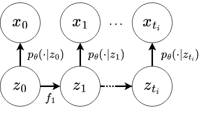
(b) Generative model

Figure 1: Proposed inference and generative models.

where $p$ is a simple prior distribution over $z_{0}^{i}$ (e.g. standard Gaussian) and $f_{j}$ are normalizing flows for any $j\in\{1,\dots,t_{i}\}$. The main idea is to assume that it is the distribution of the latent variables that evolves through time and we propose to model this evolution using the flows. As such, the time dependency is imposed on the latent variables and not directly on the observations. Note that the initial distribution can be chosen as complex as desired and that for any $j\in\{1,\dots,t_{i}\}$ we have access to a tractable density for $p(z_{j}^{i})$ using Eq. (2):

$$p(z_{j}^{i})=p(z_{0}^{i})\prod\limits_{l=1}^{j}\left|\det\frac{\partial f_{l}}{\partial z_{l-1}^{i}}\right|^{-1}\,.$$ (5)

In addition, the relation between two latent variables $z_{j}^{i}$ and $z_{k}^{i}$ with $j,k\in\{0,\dots,t_{i}\}$ such that $j<k$ is explicit and completely deterministic since we have:

$$z_{k}^{i}=\bigcirc_{l={j+1}}^{k}f_{l}(z_{j}^{i})~{}\text{and}~{}z_{j}^{i}=\bigcirc_{l={k}}^{j+1}(f_{l})^{-1}(z_{k}^{i})\,.$$ (6)

Hence, we can see that given a latent vector $z_{j}^{i}$ we can now retrieve the complete sequence $(z_{0}^{i},\dots,z_{t_{i}}^{i})$ using Eq. (6). Assuming $(x_{j}^{i})_{j\in\{1,\dots,t_{i}\}}$ are independent knowing $(z_{0}^{i},\dots,z_{t_{i}}^{i})$, the conditional distribution in Eq. (3) writes

$$p_{\theta}(x_{0}^{i},\cdots,x_{t_{i}}^{i}|z_{j}^{i})=\prod\limits_{l=0}^{t_{i}}p_{\theta}(x_{l}^{i}|z_{j}^{i})=\prod\limits_{l=0}^{t_{i}}p_{\theta}(x_{l}^{i}|z_{l}^{i})\,.$$ (7)

Using Eq. (5) and Eq. (7) allows to derive another expression of the joint distribution of the observations:

$$p_{\theta}(x_{0}^{i},\cdots,x_{t_{i}}^{i})=\int_{\mathcal{Z}}\prod\limits_{l=0}^{t_{i}}p_{\theta}(x_{l}^{i}|z_{l}^{i})p(z_{j}^{i})dz_{j}^{i}\,.$$ (8)

Since this integral is most of the time intractable, we propose to rely on variational inference (Jordan et al., 1999). We indeed introduce a parametrized variational distribution $q_{\phi}(z_{j}^{i}|x_{j}^{i})$ such that we can obtain an unbiased estimate of the joint likelihood:

$$\mathbb{E}_{q_{\phi}}\Bigg{[}\frac{\prod\limits_{l=0}^{t_{i}}p_{\theta}(x_{l}^{i}|z_{l}^{i})p(z_{j}^{i})}{q_{\phi}(z_{j}^{i}|x_{j}^{i})}\Bigg{]} =p_{\theta}(x_{0}^{i},\cdots,x_{t_{i}}^{i})\,.$$ (9)

Using Jensen’s inequality allows to derive a lower bound (ELBO) on the true objective i.e. the log joint likelihood :

$$\log~{}p_{\theta}(x_{0}^{i},\cdots,x_{t_{i}}^{i})=\log\mathbb{E}_{q_{\phi}}\Bigg{[}\frac{\prod\limits_{l=0}^{t_{i}}p_{\theta}(x_{l}^{i}|z_{l}^{i})p(z_{j}^{i})}{q_{\phi}(z_{j}^{i}|x_{j}^{i})}\Bigg{]} \geq\mathbb{E}_{q_{\phi}}\log\Bigg{[}\frac{\prod\limits_{l=0}^{t_{i}}p_{\theta}(x_{l}^{i}|z_{l}^{i})p(z_{j}^{i})}{q_{\phi}(z_{j}^{i}|x_{j}^{i})}\Bigg{]}\,,$$ (10)

$$\geq\mathbb{E}_{q_{\phi}}\log\prod\limits_{l=0}^{t_{i}}p_{\theta}(x_{l}^{i}|z_{l}^{i})-\mathrm{KL}(q_{\phi}(z_{j}^{i}|x_{j}^{i})|p(z_{j}^{i}))\,.$$

Algorithm 1 Training Procedure

  Input: Observations $(x_{0}^{i},\cdots,x_{t_{i}}^{i})$

  while not converged do

     Pick $j\in\{0,\dots,t_{i}\}$ randomly 

     $z_{j}^{i}\sim q_{\phi}(\cdot|x_{j}^{i})$ 

     for $l=j+1$ to $t_{i}$ do

        $z_{l}^{i}=f_{l}(z_{l-1})$ {propagate in future} 

     end for

     for $l=j-1$ to $0$ do

        $z_{l}^{i}=(f_{l+1})^{-1}(z_{l+1})$   {propagate in past}

     end for

     $\mathcal{L}=-\frac{1}{t_{i}+1}\sum\limits_{l=0}^{t_{i}}\log p_{\theta}(x_{l}^{i}|z_{l}^{i})+\log q_{\phi}(z_{j}^{i}|x_{j}^{i})-\log p(z_{0}^{i})-\sum\limits_{l=1}^{j}\log\Big{|}\det\frac{\partial(f_{l})^{-1}}{\partial z_{l}^{i}}\Big{|}$

  end while

The graphical models for the proposed method can be found in Fig. 1. In practice and inspired from the VAE framework, the variational distribution is chosen as a multivariate Gaussian distribution $q_{\phi}(z_{j}^{i}|x_{j}^{i})=\mathcal{N}(z_{j}^{i};\mu_{\phi}(x_{j}^{i}),\Sigma_{\phi}(x_{j}^{i}))$ for $j\in\{0,\dots,t_{i}\}$ and where $\mu_{\phi}$ and $\Sigma_{\phi}$ are given by neural networks and $\Sigma_{\phi}$ is chosen as a diagonal matrix. The conditional distributions $p_{\theta}(x_{j}^{i}|z_{j}^{i})$ are chosen depending on the input data (e.g. multivariate Gaussians for RGB images) and $p(z_{j}^{i})$ is given by Eq. (5). To mitigate the impact of the sequence length on the ELBO in Eq. (10), we average the left hand side term over the sequence length. This impedes the reconstruction term to over-weight the KL for long sequences. As for the normalizing flows, in this paper, we use Inverse Autoregressive Flows (IAF) (Kingma et al., 2016) with MADE (Germain et al., 2015) for the autoregressive networks since we need a tractable inverse. It should be noted that for such flows the computation of the inverse is however sequential and its time proportional to the dimensionality of the latent variables due to the autoregressive property of the flows. Nonetheless, in practice the dimension of the latent variables is often much smaller than the dimensionality of the input data making this choice reasonable. We choose IAF over MAF (Papamakarios et al., 2017) so that the generation of a synthetic sequence from the prior $z_{0}\sim p(z_{0})$ is fast since it does not require inverting the flows. Finally, a pseudo code of the training algorithm is provided in Alg. 1 and an implementation using PyTorch (Paszke et al., 2017) and based on (Chadebec et al., 2022b) is made available in the supplementary materials.

3.3 Dealing with Missing Data in the Sequence

In real-life applications, it is not rare to find sequences with missing observations (e.g. in medicine a loss of patient follow-up or a patient not coming to a specific visit induces missing observations for the patient’s evolution). As explained above and shown in Alg. 1, during training we perform variational inference using only one element in the sequence. Thus, the training can be modified pretty easily to handle such missing data in the input sequences and consists in only using the observed data.

Nonetheless, this can be seen as a weakness of the method at inference time. Let us indeed imagine that we are given a sequence of 5 measure times $(x_{0}^{i},x_{1}^{i},x_{2}^{i},x_{3}^{i},x_{4}^{i})$ where only 3 are actually observed, say $x_{1}^{i},x_{2}^{i}$ and $x_{4}^{i}$. In its current shape, during inference, the method will choose an observation time $j\in\{1,2,4\}$, say $j=2$, sample a latent variable associated to observation $x_{2}^{i}$ using the approximate posterior $q_{\phi}(\cdot|x_{2}^{i})$ and then generate a sequence $(z_{l}^{i})_{l\in\{0,\dots,4\}}$ using the learned flows. This sequence is then used to sample a reconstructed sequence in the observations space using $p_{\theta}(x|z)$. This is actually sub-optimal since this would be equivalent to only have access to observation $x_{2}^{i}$ without benefiting from the information provided by $x_{1}^{i}$ and $x_{4}^{i}$. In order to address this potential limitation of the model, we propose to generate a sequence (actually we can generate an arbitrary number of sequences) for each index corresponding to an observed input data in the sequence (i.e. $\{1,2,4\}$ in the example) and keep the generated sequence achieving the highest likelihood on the observed data. In other words, if we denote $\mathcal{O}_{i}$ the set of observed indices in the input sequence, we define the optimal index that should be used to complete the sequence as follows:

$$j_{\mathrm{opt}}=\arg\max_{j\in\mathcal{O}_{i}}\sum\limits_{l\in\mathcal{O}_{i}}\log p_{\theta}(x_{l,j}^{i}|z_{l,j}^{i})\,,$$ (11)

where $z_{l,j}^{i}$ is the latent variable and $x_{l,j}^{i}$ the data generated at time $l$ using index $j$. Alg. 2 shows the inference procedure.

Algorithm 2 Inference Procedure for Missing Observations

  Input: A sequence $(x^{i}_{j})_{j\in\mathcal{O}_{i}}$ with missing observations

  for $j\in\mathcal{O}_{i}$ do

     $z_{j,j}^{i}\sim q_{\phi}(\cdot|x_{j}^{i})$ 

     $\hat{x}_{j,j}^{i}\sim p_{\theta}(\cdot|z_{j,j}^{i})$ 

     for $l=j+1$ to $t_{i}$ do

        $z_{l,j}^{i}=f_{l}(z_{l-1,j})$  

        $\hat{x}_{l,j}^{i}\sim p_{\theta}(\cdot|z_{l,j}^{i})$ 

     end for

     for $l=j-1$ to $0$ do

        $z_{l,j}^{i}=(f_{l+1})^{-1}(z_{l+1,j})$  

        $\hat{x}_{l,j}^{i}\sim p_{\theta}(\cdot|z_{l,j}^{i})$ 

     end for

  end for

  $j_{\mathrm{opt}}=\arg\max\limits_{j\in\mathcal{O}_{i}}\sum\limits_{l\in\mathcal{O}_{i}}\log p_{\theta}(x_{l,j}^{i}|z_{l,j}^{i})$

  return $(\hat{x}_{0,j_{\mathrm{opt}}}^{i},\cdots,\hat{x}_{t_{i},j_{\mathrm{opt}}}^{i})$ {obtained with $j_{\mathrm{opt}}$}

3.4 Enhancing the Model

One interesting aspect of the model is that one may use improvements that have been proposed and proved useful in the literature related to variational inference and VAEs to enhance several part of the model independently.

Improving the prior

Even-though, a simple distribution such as a standard Gaussian appeared to work well in practice, a smarter choice in the prior distribution may result in an enhanced data generation or better likelihood estimates (Hoffman & Johnson, 2016). As such, richer priors (Nalisnick et al., 2016; Dilokthanakul et al., 2017) or priors that are learned (Chen et al., 2016; Razavi et al., 2020; Pang et al., 2020; Aneja et al., 2020) can be easily plugged into our model. We show in the experiments section how changing the prior from a standard Gaussian to a VAMP prior (Tomczak & Welling, 2018) can influence the results.

Improving the variational bound

Following (Rezende & Mohamed, 2015) insights, another way to improve the expressiveness of the model and ideally achieve a tighter ELBO consists in enriching the potentially too simplistic parameterised variational distribution $q_{\phi}(z|x)$ using flows. This improvement can be easily integrated within our framework as well. In the experiments section, we also propose a variant model where the posterior distributions are enriched using IAF flows as proposed in (Kingma et al., 2016). Methods proposing to use MCMC sampling steps with learned Markov kernels (Salimans et al., 2015) or relying on Hamiltonian dynamics (Caterini et al., 2018; Chadebec et al., 2022a) could also be envisioned but are not tested in combination with our model due to the strong computation burden they imply.

4 Related Works

Variational Autoencoders (VAEs) (Kingma & Welling, 2014; Rezende et al., 2014) share some aspects with our method. First, they try to maximise the likelihood of a set of data using a variational approach. Second, they try to take advantage of the flexibility a latent space provides by mapping potentially high dimensional input data into a lower dimensional space. However, they assume that the input data are independent and so are the latent variables. This impedes the model to capture the potentially complex time dependency that exists with longitudinal data.

There exist however some works on VAEs that are worth citing since they stress the flexibility offered by considering a latent space. In particular, they motivated our idea to impose the time dependency over the latent variables and not directly on the observations. First, several papers argued that the latent space of the VAE can reveal representative and interpretable features through its ability to perform disentanglement (Higgins et al., 2017; Burgess, 2018; Korkinof et al., 2018; Chen et al., 2018b). Studying the latent space with a geometric point of view, other works showed that this latent space can actually be modelled with a specific geometry (e.g. hyper-sphere, Poincaré Disk, Riemannian manifold) (Davidson et al., 2018; Falorsi et al., 2018; Mathieu et al., 2019; Kalatzis et al., 2020; Chadebec et al., 2022a) or that a Riemannian geometry can naturally arise in the latent space (Arvanitidis et al., 2018; Chen et al., 2018a; Shao et al., 2018; Chadebec & Allassonnière, 2022). Finally, another way to enhance the representation capability of the model that was proposed in the literature consists in increasing the expressiveness of the variational posterior distribution using MCMC sampling (Salimans et al., 2015) or normalizing flows (Rezende & Mohamed, 2015).

Arguing that VAEs still fail to capture complex correlations, there were some proposals in the literature trying to constraint the model to account for these correlations in the latent space. For instance, the conditional VAE (Sohn et al., 2015) feeds auxiliary variables directly to the encoder and decoder networks but fails to model the evolution of a given subject through time. Gaussian processes that are a powerful tool for time series (Seeger, 2004; Roberts et al., 2013) were also proposed as prior for the VAE (Casale et al., 2018; Fortuin et al., 2020) to account for the temporal structure across the samples. (Ramchandran et al., 2021) enriched these models with the inclusion of covariates different from time using a multi-output additive Gaussian process prior.

Also closely related to our method are approaches involving neural ordinary differential equations (NODE) that see the forward pass of a residual network as solving an ODE (Chen et al., 2018c), an approach that was for instance extended in (Dupont et al., 2019; Rubanova et al., 2019; Massaroli et al., 2020). In particular, the latent neural ODE model proposed in (Chen et al., 2018c) defines a generative model by assuming that the initial state latent variable follows a given prior distribution and a latent trajectory is then obtained by solving an ODE. The model also relies on variational inference but considers an approximate posterior conditioned on the entire input sequence leading to very different latent representations when compared to our method. The idea was further enriched in (Rubanova et al., 2019) to handle irregularly-sampled time series and extended to SDE in (Chung et al., 2015; Serban et al., 2017). However, these models were rarely used on high dimensional sequences such as images while the method we propose appears well suited for such type of data. We can nonetheless cite (Kanaa et al., 2021; Park et al., 2021) but that only validated their method on simple databases and (Yildiz et al., 2019) that proposed to optimize a complex loss function and to rely on adversarial training making the training procedure tricky. Moreover, these works were mainly designed for conditional generation (prediction of future time points or interpolation), while the usability of these methods for unconditional generation remains to be proven.

Modelling longitudinal data and trying to understand the underlying evolution dynamic is something that has also been quite studied under the prism of disease progression modelling (Jedynak et al., 2012; Fonteijn et al., 2012). In such literature, mixed-effect models (Laird & Ware, 1982) that parameterise a patient’s evolution as a deviation from a reference trajectory have become more and more popular (Diggle et al., 2002; Singer et al., 2003). First applied on Euclidean data (Bernal-Rusiel et al., 2013), they were then extended with a Riemannian geometry viewpoint (Schiratti et al., 2015; Singh et al., 2016; Koval et al., 2017; Bône et al., 2018) or combined with dimensionality reduction (Louis et al., 2019; Sauty & Durrleman, 2022). Despite being adapted to model disease progression, it is unclear how these models would apply to datasets where there is no clear average evolution.

Finally, deep learning based methods relying on recurrent neural networks are also worth citing as they revealed useful for time varying data (Pearlmutter, 1989). To cite a few, GRUI-GAN (Luo et al., 2018) and BRITS (Cao et al., 2018) were proposed with the aim of handling missing data but with the drawback of relying on adversarial training for the first one and not being generative for the second. (Chung et al., 2015) proposed a combination of VAE and RNN for structured sequential data but there exists no clear way how the model would handle missing data.

5 Experiments

In this section, we validate the proposed method through series of experiments. We place ourselves in the context of high-dimensional data (images) and so set $d\ll D$ (i.e. the latent variables live in a much lower-dimensional latent space when compared to the input images size). In line with the VAE framework, the inference network providing the parameters of the variational distribution $q_{\phi}(z|x)$ can then be interpreted as an encoder and the generative model $p_{\theta}(x|z)$ as a decoder. Note that neither the encoder nor the decoder depend on time. First, we show that the proposed model is able to achieve better joint likelihood estimates than several models proposed in the literature on 5 datasets. Then, we show that the method is also able to impute missing data (and features) and compare its performances in term of reconstruction with benchmark models. Finally, we evaluate the ability of the proposed model to generate relevant conditioned and fully synthetic sequences. We also conduct in Appendix E an ablation study stressing the influence of the flows, latent space dimension and prior complexity and discuss the relevance of Eq. (11) for missing data imputation in Appendix F.

Table 1: Negative log joint likelihood divided by the sequence length computed on an independent test set with 5 independent runs and 100 importance samples.

Model	Starmen	RotMNIST	ColorMNIST	3d chairs	Sprites
VAE	3781.82 $\pm$ 0.01	741.03 $\pm$ 0.00	2179.88 $\pm$ 0.00	11359.39 $\boldsymbol{\pm}$ 0.02	11313.38 $\pm$ 0.00
VAMP	3780.99 $\pm$ 0.01	740.82 $\pm$ 0.00	2179.60 $\pm$ 0.00	11361.01 $\pm$ 0.02	11313.43 $\pm$ 0.00
TVAE (0)	3806.26 $\pm$ 0.07	748.18 $\pm$ 0.00	2185.40 $\pm$ 0.00	11419.32 $\pm$ 0.11	11332.09 $\pm$ 0.01
TVAE (short)	3782.39 $\pm$ 0.05	744.07 $\pm$ 0.00	2175.54 $\pm$ 0.00	11373.76 $\pm$ 0.07	11318.96 $\pm$ 0.01
TVAE (part)	3780.75 $\pm$ 0.05	739.53 $\pm$ 0.00	2174.19 $\pm$ 0.00	11364.21 $\pm$ 0.18	11308.40 $\pm$ 0.01
TVAE (half)	3777.57 $\pm$ 0.07	745.55 $\pm$ 0.00	2173.58 $\pm$ 0.00	11363.27 $\pm$ 0.12	11305.62 $\pm$ 0.01
BubbleVAE	3780.46 $\pm$ 0.07	742.66 $\pm$ 0.00	2174.74 $\pm$ 0.00	11369.59 $\pm$ 0.19	11310.69 $\pm$ 0.01
GPVAE (Cauchy)	3780.36 $\pm$ 0.03	740.05 $\pm$ 0.00	2177.21 $\pm$ 0.00	11367.43 $\pm$ 0.02	11309.11 $\pm$ 0.01
GPVAE (rbf)	3787.80 $\pm$ 0.03	745.58 $\pm$ 0.00	2187.15 $\pm$ 0.00	11390.33 $\pm$ 0.04	11315.68 $\pm$ 0.01
GPVAE (diffusion)	3780.96 $\pm$ 0.01	740.26 $\pm$ 0.00	2178.63 $\pm$ 0.00	11359.21 $\boldsymbol{\pm}$ 0.00	11312.50 $\pm$ 0.00
GPVAE - matern	3779.29 $\pm$ 0.02	739.68 $\pm$ 0.00	2176.63 $\pm$ 0.00	11360.36 $\pm$ 0.03	11309.90 $\pm$ 0.00
Ours ($\mathcal{N}$)	3773.23 $\pm$ 0.17	735.71 $\pm$ 0.00	2173.16 $\pm$ 0.05	11362.00 $\pm$ 0.62	11301.51 $\pm$ 0.04
Ours (VAMP)	3772.91 $\boldsymbol{\pm}$ 0.16	736.15 $\pm$ 0.00	2173.00 $\pm$ 0.05	11364.73 $\pm$ 0.51	11301.30 $\boldsymbol{\pm}$ 0.02
Ours (IAF)	3773.01 $\boldsymbol{\pm}$ 0.17	735.27 $\boldsymbol{\pm}$ 0.01	2172.85 $\boldsymbol{\pm}$ 0.05	11359.48 $\boldsymbol{\pm}$ 0.67	11301.97 $\pm$ 0.02

5.1 Data

For these experiments, we consider 5 different databases that mimic longitudinal datasets. The first one is a synthetic longitudinal dataset composed of 1,000, 64x64 images of starmen raising their left arm and generated according to the diffeomorphic model of (Bône et al., 2018). The second one consists of 8 evenly separated rotations applied to the MNIST database (LeCun, 1998) from 0 to 360 degrees, we call it rotMNIST. In addition to these two toy datasets, we also consider more challenging ones. The third one called colorMNIST is created using the approach of (Keller & Welling, 2021). It consists of sequences of colored MNIST digits that can undergo three distinct types of transformations: color change (from turquoise to yellow), scale change or rotations. It is important to note that for this database, the time dynamic cannot be fully recovered from a single image since it can correspond to different transformations. For instance, a starting turquoise 6 can either change of color or undergo a change in scale. The fourth database is created using the 3d chairs dataset (Aubry et al., 2014) consisting of 3D CAD chair models and considering as input sequences, 11 evenly separated rotations of a chair (from 0 to 360^∘). Finally, we use the sprites dataset (Li & Mandt, 2018) consisting of 64x64 RGB images of characters performing actions such as dancing or walking. Find more details about the datasets, potential pre-processing steps and some examples of the training sequences in Appendix. A.

5.2 Likelihood Estimation

First, we compare the proposed model and two of its variants (using either a VAMP prior or IAF flows to enrich the posterior approximation) to a vanilla VAE (Kingma & Ba, 2014), a VAE with a VAMP prior (Tomczak & Welling, 2018) and models incorporating temporal coherence such as the BubbleVAE (Hyvärinen et al., 2004) or the Topographic VAE (TVAE) (Keller & Welling, 2021). For the latter, we consider several models with different temporal coherence length $L$: TVAE (0) i.e. no temporal coherence, TVAE (short) i.e. $L\approx\frac{1}{8}$ of the input sequence length $S$, TVAE (part) where $L\approx\frac{1}{4}S$ and TVAE (half) with $L=\frac{1}{2}S$, i.e. the model takes into account the full sequence. We also compare our model to a VAE using a Gaussian Process as prior (GPVAE) proposed in (Fortuin et al., 2020). For this model, we consider several GP kernels (RBF, Cauchy, diffusion and matern). We use the 5 datasets presented in the previous section and train all the models on a train set, keep the best model on a validation set and compute the negative log joint-likelihood on an independent test set using 100 importance samples in a similar fashion as (Burda et al., 2016). We train the models for 200 epochs for sprites and rotMNIST, 250 for colorMNIST and 400 for starmen and chairs with a latent dimension set to 16 for all datasets but for the 3d chairs dataset where it is set to 32. Any other relevant piece of information about training configurations is provided in Appendix D. We show in Table 1, the mean and standard deviation of the negative log joint likelihood obtained with 5 independent runs. For all datasets, the model is able to either compete or outperform the competitors. Moreover, as expected, using a richer prior (VAMP) or enriching the expressiveness of the variational posterior with flows (IAF) leads most of the time to a better likelihood estimation. This is an encouraging aspect since it shows that the model can be improved pretty easily using independent bricks available in the variational inference literature.

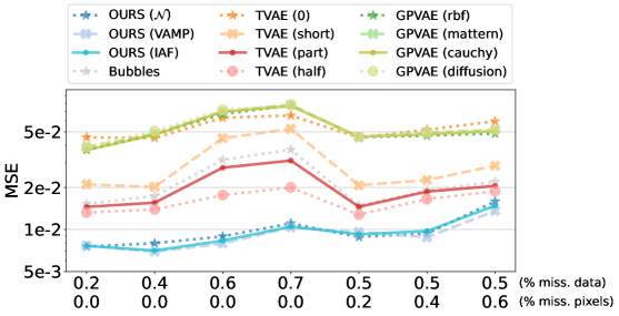
(a)

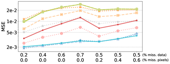
(b)

Figure 2: Mean Square Error (MSE) on the test data for different proportions of missing observations (0.2 to 0.7) and missing pixels (0.2 to 0.6) in the input train, validation and test sequences for the starmen (top) and sprites (bottom) datasets. The proposed model appears very robust to incomplete sequences thanks to the flows-based structure.

5.3 Missing Data Imputation

The second experiment that we conduct consists in assessing the robustness of the model when it faces missing data and test its ability to impute missing values. To do so we consider 2 databases: starmen and sprites; and randomly remove observations in input sequences with probability 0.2, 0.4, 0.6 and 0.7. To challenge the model in the context of missing features, we also create sequences with missing observations (randomly removed with probability 0.5) and missing pixels in the observed images (randomly removed with probability 0.2, 0.4 and 0.6). All the models are trained with the same masks and are optimised using an objective computed only on the seen pixels. The charts in Fig. 2 show the Mean Square Error (MSE) obtained on an independent test set. In all scenarios, the proposed model outperforms the TVAEs, BubbleVAEs and GPVAEs and appears as expected quite robust to missing observations in the input sequences. This is made possible thanks to the training structure that uses only one seen observation to perform variational inference.

In Fig. 3, we also show some conditional generations obtained with the proposed model on the colorMNIST dataset. At the top, we show 5 generated trajectories using 2 different images. In each case, we draw 5 random latent variables from the corresponding variational posterior $q_{\phi}(z|x)$. They are then passed through the flows according to Eq. (4) leading to 5 sequences and finally decoded using $p_{\theta}(x|z)$. In a), the model is able to produce a range of possible evolutions (changes of color or scale) that are plausible given the dataset considered. This is a very important property of the model since thanks to the variational posterior distribution it can generate an infinite number of possible trajectories from a single observation. Moreover, we see that the model is clearly able to keep the shape coherence all along the trajectory. At the bottom, we show the sequences obtained by using each image available in the sequence (not greyed). We rank the generated trajectories as they maximise the likelihood on the seen data (i.e. according to Eq. (11)). This experiment shows how the model can benefit from the information available in the sequence despite only using one image to generate. In practice, one may generate as many trajectories as desired for each image available in the sequence (and not just one as in this example) and chose the one that maximises Eq. (11). As a conclusion, these experiments show that even-though the relation between the latent variables of a sequence is deterministic, the stochasticity in the conditionally generated sequences arises from the sampling from the variational posterior that is able to capture the modularity of the data.

(a)

(b)

(c)

(d)

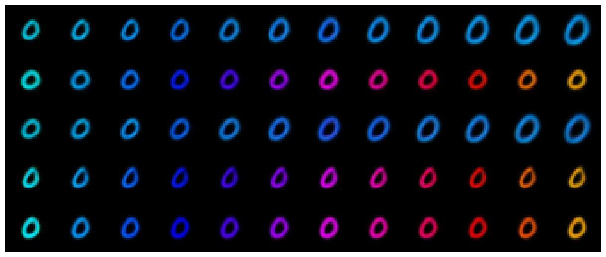
(e) (a)

(f) (b)

(g) (a)

(h) (b)

Figure 3: Conditionally generated trajectories (greyed are unseen data). Left: 5 generated sequences using the same input image. For each trajectory, 5 latent variables are drawn from the posterior distribution $q_{\phi}(z|x)$, passed trough the flows and decoded using $p_{\theta}(x|x)$. In a), the model is able to produce possible evolutions (changes of color or scale) for the dataset considered. Right: Generated sequences using each seen data in the input sequence. The generated sequences are ranked as they maximise the likelihood on the seen data according to Eq. (11) (best at the top).

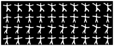
(a)

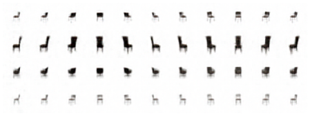
(b)

(c)

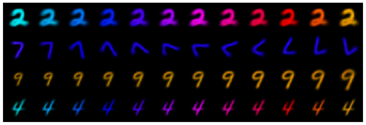
(d)

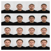
(e)

Figure 4: Generated sequences using the proposed model. Latent variables are sampled from the prior distribution (taken as a standard Gaussian in this example) and propagated through the flows according to Eq. (4). The obtained latent sequences are then decoded using the conditional distribution $p_{\theta}(x|z)$ to create the image sequences.

5.4 Unconditional Sequence Generation

In this section, we evaluate the ability of the proposed model to generate relevant fully synthetic trajectories. For this experiment, we first compute the Frechet Inception Distance (FID) (Heusel et al., 2017) on the colorMNIST and sprites datasets. The FID is computed by generating the same number of images as available in an independent test set: 21,312 for sprites (2,664 sequences of 8 time steps) and 120,000 for colorMNIST. Note that in this setting the FID does not account for the temporal coherence between the generated samples within a sequence. As shown in Table 2, the proposed model achieves the lowest FID (lower is better). The fact that it is able to outperform a VAE or a VAMP-VAE shows that the temporal coherence constraint imposed by the flows does not affect the quality of the generated images. Moreover, we see the influence of using a more complex prior or enriching the variational approximation on the generative capability of the model that can achieve better FIDs. Finally, we show generated samples for the 3d chairs, starmen, sprites, colorMNIST and the Radboud Faces Database consisting of 67 individuals displaying different emotions (Langner et al., 2010). For the latter dataset, we create sequences of 4 time steps corresponding to the emotions: anger, happiness, sadness and surprise; and down-sample the images so they are of size 64x64. We show 4 generated sequences for each dataset in Fig. 4. Thanks to the flow-based structure, the model is able to generate relevant sequences that clearly keep a temporal consistency. Additional samples can be found in Appendix B and small movies in the supplementary materials. We also show that the proposed model does not simply memorise the training samples by showing the closest training sequence to the generated ones in Fig. 5 and Appendix C.

Table 2: FID (lower is better) computed on an independent test set with the same number of generated samples as available in the test set.

Model	ColorMNIST	Sprites
VAE	29.79	53.37
VAMP	33.92	59.85
GPVAE	31.93	56.74
Ours ($\mathcal{N}$)	28.62	44.82
Ours (VAMP)	25.07	40.23
Ours (IAF)	28.14	41.81

6 Conclusion

In this paper, we introduced a new generative model for longitudinal data that relies on variational inference and normalizing flows. It proved able to generate relevant fully synthetic sequences and to propose plausible trajectories when conditioned on one or several seen samples in an input sequence. We also discussed and showed that our model can benefit from improvements proposed in the variational inference literature. In particular, we proposed two variants of our model using either a more complex prior or a more flexible variational posterior using flows. These independent enhancements revealed particularly useful for likelihood estimation and unconditional generations. Moreover, the proposed model demonstrated quite a good robustness to missing data and showed to be useful for missing data imputation. Nonetheless, a potential weakness of the model is that the flow-based structure makes it discrete. Furthermore, we acknowledge that the deterministic aspect induced by the choice of normalizing flows to account for time dependency in the latent space can be seen as a limitation to the expressiveness of the model. In particular, future work may involve stochastic trajectories in a spirit similar to latent SDEs, which would add to the expressiveness of the model. Nevertheless, such determinism in trajectories combined with the proposed training scheme may also benefit the posterior variational distributions that are constrained to be sufficiently expressive to capture the stochasticity of the trajectories.

Gen. Train
Gen. Train

(a)

(b)

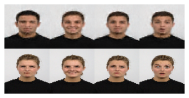
(c)

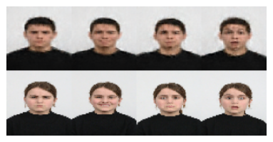
(d)

Figure 5: Closest train sequences (train) to the generated ones (gen.). See more examples in Appendix C.

Appendix A The Data

In this section, we display some training samples for each dataset used in the paper. We recall that the first one shown in Fig. 6a is a synthetic longitudinal dataset composed of 1,000, 64x64 images of starmen raising their left arm and generated according to the diffeomorphic model of (Bône et al., 2018). The second one shown in Fig. 6b consists of 8 evenly separated rotations applied to the MNIST database (LeCun, 1998) from 0 to 360 degrees. The third one called colorMNIST is created using the approach of (Keller & Welling, 2021). It consists of sequences of colored MNIST digits that can undergo three distinct types of transformations: color change (from turquoise to yellow), scale change or rotations and is presented in Fig. 6c. It is important to note that for this database, the time dynamic cannot be fully recovered from a single image since it can correspond to different transformations. For instance, a starting turquoise 6 can either change of color or undergo a change in scale as shown on line 2 and 3 of Fig. 6c. The fourth database is created using the 3d chairs dataset (Aubry et al., 2014) consisting of 3D CAD chair models and considering as input sequences, 11 evenly separated rotations of a chair (from 0 to 360^∘). Some samples are displayed in Fig. 6e. We also use the sprites dataset (Li & Mandt, 2018) shown in Fig. 6f that consists of 64x64 RGB images of characters performing actions such as dancing or walking. Finally, we also consider the Radboud Faces Database consisting of 67 individuals expressing different emotions (Langner et al., 2010). For this dataset, we create sequences of 4 time steps corresponding to the emotions: anger, happiness, sadness and surprise; and down-sample the images so they are of size 64x64 as shown in Fig. 6d.

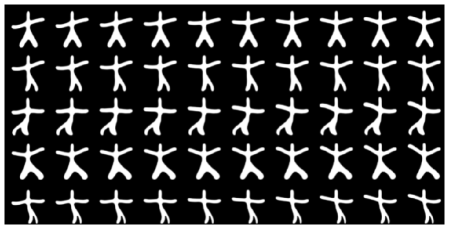
(a) Starmen

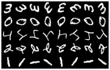
(b) rotMNIST

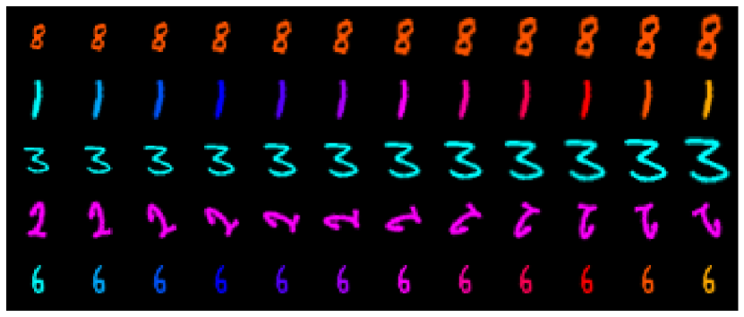
(c) colorMNIST

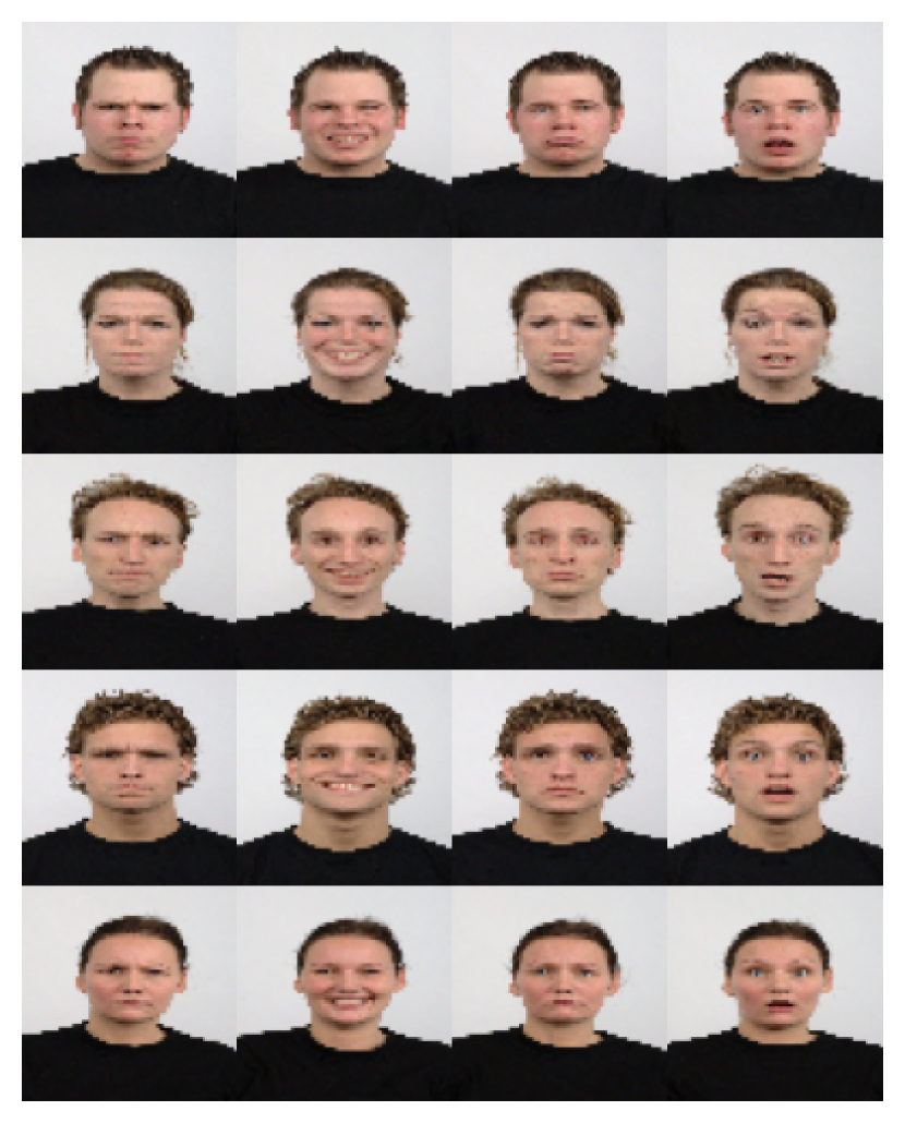
(d) Faces

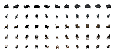
(e) 3d chairs

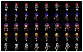
(f) Sprites

Figure 6: 5 training sequences for each dataset considered in the paper.

Appendix B Some More Generations

In this section, we show 20 additional generated sequences for the starmen dataset in Fig. 7, the colorMNIST dataset in Fig. 8, the sprites data in Fig. 9, the faces dataset in Fig. 10 and the chairs dataset in Fig. 11. This experiment shows the diversity of the generated trajectories as well as their relevance.

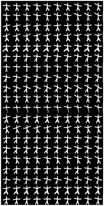
Figure 7: 20 sequences generated by our model trained on the starmen dataset.

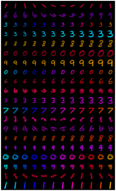
Figure 8: 20 sequences generated by our model trained on the colorMNIST dataset.

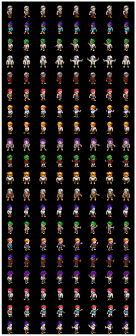
Figure 9: 20 sequences generated by our model trained on the sprites dataset.

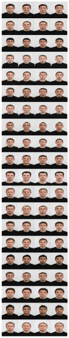
Figure 10: 20 sequences generated by our model trained on the faces dataset.

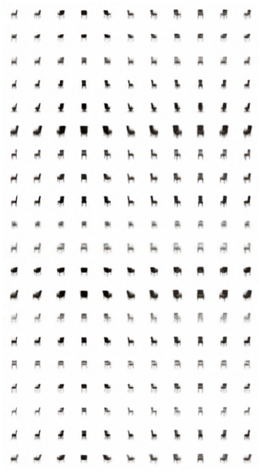
Figure 11: 20 sequences generated by our model trained on the chairs dataset.

Appendix C Exploring Overfitting

In this section, we show that the proposed model generates unseen sequences by comparing 4 generated trajectories to the closest one in the train set (using L2 norm). For each dataset, we see that the generated sequence is different from the training data. For instance, for the starmen, the individual has a different shape while for the sprites, the individual has different pants, hair or top’s color.

Gen Train
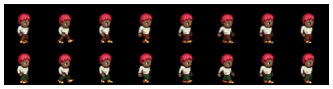
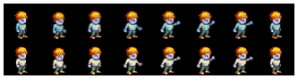
Gen. Train
Gen. Train
Gen. Train
Gen. Train
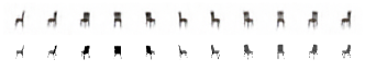
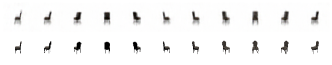
Gen. Train
Gen. Train

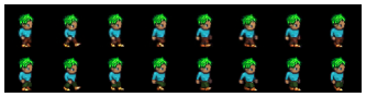
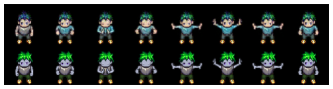
(a) (a)

(b) (b)

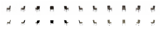
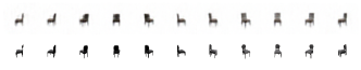
(c) (c)

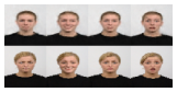
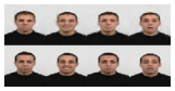
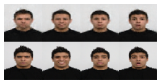
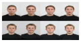
(d) (d)

Figure 12: Closest train sequences (train) to the generated ones (gen.) using our model trained on (a) the sprites, (b) starmen, (c) 3d chairs and (d) faces datasets.

Appendix D Experimental Details

In this section, we detail all the relevant parameters we used for the experiments. The datasets presented in Appendix A are first split into a train set, a validation set and a test set as shown in Table 3. We train the models for 200 epochs for sprites and rotMNIST, 250 for colorMNIST and 400 for starmen and chairs with a latent dimension set to 16 for all datasets but for the chairs dataset where it is set to 32. We select the model achieving the lowest validation loss in each case. We use the Adam optimiser (Kingma & Ba, 2014) with a starting learning rate of $10^{-3}$ together with schedulers reducing the learning rate by a factor $0.5$ at epoch 50, 100, 125 and 150 for starmen, by a factor $10^{-4}$ at epoch 50, 75, 100, 125 and 150 for rotMNIST, by a factor $10^{-4}$ at epoch 50, 100, 150 and 200 for colorMNIST, by a factor $0.5$ at epoch 150, 200, 250, 300 and 350 for 3d chairs and a factor $0.5$ at epoch 50, 100, 125 and 150 for sprites. For the faces dataset we use a scheduler multiplying the learning rate by $10^{-6}$ every 2,000 epochs and train the model for 10,000 epochs. We use a batch of size 128 for rotMNIST, colorMNIST and faces and 64 otherwise. For the proposed model, we also use 10 warm-up epochs where we train it like a VAE to stabilise the encoder and decoder networks and ease the learning of the flows. This hyper-parameter does not influence much the performances as shown in Appendix E. The flows are implemented using (Chadebec et al., 2022b) and are composed of 2 IAF blocks using 3-layer MADE (Germain et al., 2015) with 128 hidden units. For the variants of our model, we use 500 components in the VAMP prior and IAF flows are composed of 3 IAF transformations using 2-layer MADE with 128 hidden units. All models are trained on a single 32-GB V100 GPU and the FID metrics are computed using the implementation of https://github.com/mseitzer/pytorch-fid. Finally, we provide the neural networks we use in Table 4. For faces we use the same networks as for sprites dataset.

Datasets	Train	Validation	Test
Starmen	700	200	100
rotMNIST	9,000	1,000	10,000
colorMNIST	48,000	12,000	10,000
sprites	8,000	1,000	2,664
3d chairs	1,000	200	193

Table 3: Number of sequences considered in the Train/Val/Test splits used in the experiments.

Dataset	Starmen	rotMNIST	colorMNIST	3d chairs	Sprites
Input dimension	(1, 64, 64)	(1, 28, 28),	(3, 28, 28)	(3, 64, 64)	(3, 64, 64)
	Conv2D(1, 16, 4, 2)	Linear(1024)	Linear(1024)	Conv2D(3, 16, 4, 2)	Conv2D(3, 16, 4, 2)
	Conv2D(16, 32, 4, 2)	ReLU	ReLU	Conv2D(16, 32, 4, 2)	Conv2D(16, 32, 4, 2)
	LeakyReLU	Linear(256)	Linear(256)	LeakyReLU	LeakyReLU
Inference	Conv2D(32, 64, 3, 2)	ReLU	ReLU	Conv2D(32, 64, 3, 2)	Conv2D(32, 64, 3, 2)
Network	LeakyReLU	Linear(2x16)∗	Linear(2x16)∗	LeakyReLU	LeakyReLU
	Conv2D(64, 128, 3, 2)	-	-	Conv2D(64, 128, 3, 2)	Conv2D(64, 128, 3, 2)
	LeakyReLU	-	-	LeakyReLU	LeakyReLU
	6 ResBlocks	-	-	6 ResBlocks	6 ResBlocks
	Linear (2048, 2x16)∗	-	-	Linear (2048, 2x32)∗	Linear (2048, 2x16)∗
Input dimension	16	16	16	32	16
	Linear(2048)	Linear(256)	Linear(256)	Linear(2048)	Linear(2048)
	ConvT(128, 3, 2)	ReLU	ReLU	ConvT(128, 3, 2)	ConvT(128, 3, 2)
	6 ResBlocks	Linear(1024)	Linear(1024)	6 ResBlocks	6 ResBlocks
	ConvT(64, 5, 2)	ReLU	ReLU	ConvT(64, 5, 2)	ConvT(64, 5, 2)
Generative	LeakyReLU	Linear(784)	Linear(2352)	LeakyReLU	LeakyReLU
Network	ConvT(32, 5, 2)	Sigmoid	Sigmoid	ConvT(32, 5, 2)	ConvT(32, 5, 2)
	LeakyReLU	-	-	LeakyReLU	LeakyReLU
	ConvT(16, 4, 2)	-	-	ConvT(16, 4, 2)	ConvT(16, 4, 2)
	LeakyReLU	-	-	LeakyReLU	LeakyReLU
	ConvT(1, 4, 2)	-	-	ConvT(3, 4, 2)	ConvT(3, 4, 2)
*Layer outputting the mean and covariance of the variational posterior $q_{\phi}$

Table 4: Neural networks architectures used in the experiments and keep the same for all the models in the benchmarks. The ResBlocks use 2 convolution layers with kernel of size 3 and 1, 32 channels and stride 1.

Appendix E Ablation Study

In this section, we present an ablation study of the proposed model where we study the influence of the flow complexity, the latent space dimension, the number of warm-up steps (when the model is trained as a VAE) and the prior complexity. We see in Table 6 and Table 6 that neither the choice in the flows nor the number of warm-up steps influence much the resulting likelihoods. Table 8 shows that as expected choosing a too small latent space dimension is detrimental to the model performance. Finally, Table 8 shows the influence of the prior complexity (number of components used in the VAMP prior). As expected, increasing the complexity of the prior allows achieving better likelihood estimates.

IAF	MADE	Starmen	Sprites
Blocks	layers
1	3	3774.79 $\pm$ 0.19	11302.90 $\pm$ 0.02
2	1	3773.31 $\pm$ 0.15	11302.25 $\pm$ 0.03
2	2	3774.35 $\pm$ 0.17	11301.49 $\pm$ 0.04
2	3	3773.23 $\pm$ 0.18	11301.51 $\pm$ 0.04
2	4	3773.45 $\pm$ 0.12	11302.23 $\pm$ 0.03
2	5	3773.88 $\pm$ 0.17	11301.47 $\pm$ 0.02
3	3	3773.13 $\pm$ 0.10	11302.92 $\pm$ 0.03
4	3	3774.12 $\pm$ 0.15	11301.05 $\pm$ 0.05

Table 5: Influence of the flow complexity

Warmup	Starmen	Sprites
2	3773.73 $\pm$ 0.10	11301.59 $\pm$ 0.02
5	3773.49 $\pm$ 0.10	11301.15 $\pm$ 0.03
10	3773.23 $\pm$ 0.18	11301.51 $\pm$ 0.04
20	3774.03 $\pm$ 0.10	11302.28 $\pm$ 0.03
50	3773.42 $\pm$ 0.11	11301.32 $\pm$ 0.08
100	3772.44 $\pm$ 0.12	11302.40 $\pm$ 0.06

Table 6: Influence of the warmup steps

Warmup	Starmen	Sprites
2	3817.92 $\pm$ 0.20	11346.92 $\pm$ 0.09
8	3774.20 $\pm$ 0.19	11303.18 $\pm$ 0.02
16	3773.23 $\pm$ 0.18	11301.51 $\pm$ 0.04
32	3773.16 $\pm$ 0.16	11302.23 $\pm$ 0.02
64	3773.22 $\pm$ 0.13	11301.79 $\pm$ 0.02

Table 7: Influence of the latent dimension

VAMP	Starmen	Sprites
Components
10	3773.55 $\pm$ 0.07	11302.82 $\pm$ 0.04
50	3772.71 $\pm$ 0.15	11301.26 $\pm$ 0.02
100	3772.89 $\pm$ 0.16	11302.07 $\pm$ 0.03
200	3772.66 $\pm$ 0.22	11302.03 $\pm$ 0.03
500	3772.91 $\pm$ 0.02	11301.30 $\pm$ 0.02

Table 8: Influence to the prior complexity

Appendix F Influence of Eq. (11) on Missing Data Imputation

In this appendix, we demonstrate empirically the relevance of the method proposed in Section 3.3 to handle missing observations at inference time. We recall that it consists in drawing one (or several) latent variables from the posterior associated to each data point observed in an input sequence (See Alg. 2). The latent variables are then propagated though the flows and sequences are generated in the observation space using the conditional distribution $p_{\theta}(x|z)$. Using Eq. (11), we propose to keep the trajectory achieving the highest likelihood on the observed data. This allows to benefit from all the information observed in the sequence. In Fig. 13, we show the Mean Square Error (MSE) on the missing pixels only for the starmen dataset (top) and sprites dataset (bottom). We keep the same setting as presented in the paper and remove some data in the input sequences with probability 0.2, 0.4, 0.6 and 0.7 or create sequences with missing observations (randomly removed with probability 0.5) and missing pixels in the observed images (randomly removed with probability 0.2, 0.4 and 0.6). Results obtained with the naive method that consists in using only one randomly chosen data point in the sequence to reconstruct the full sequence as done during training (see Alg. 1) are presented by the slightly transparent bars while results obtained using the method proposed in Section 3.3 are shown by the solid bars. In this example, we generate one trajectory per observed data point and keep the one achieving the highest likelihood according to Eq. (11). These graphs show the relevance of this method that allows achieving lower MSE in each scenario. Moreover, it allows to decrease significantly the standard deviation (represented by the black bar) leading to a more reliable missing data imputation.

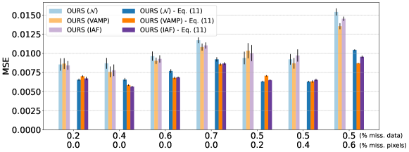
(a)

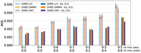
(b)

Figure 13: Mean Square Error (MSE) on missing pixels only of the test data for different proportions of missing observations (0.2 to 0.7) and missing pixels (0.2 to 0.6) in the input train, validation and test sequences for the starmen (top) and sprites (bottom) datasets. Slightly transparent bars represent the naive method (consisting in using only one randomly chosen data point in the sequence to reconstruct the full sequence as done during training) while solid bars show the results obtained using the method proposed in Section 3.3.

References

- Aghili et al. (2018) Aghili, M., Tabarestani, S., Adjouadi, M., and Adeli, E. Predictive modeling of longitudinal data for alzheimer’s disease diagnosis using rnns. In PRedictive Intelligence in MEdicine, pp. 112–119, Cham, 2018. Springer International Publishing.
- Aneja et al. (2020) Aneja, J., Schwing, A., Kautz, J., and Vahdat, A. NCP-VAE: Variational autoencoders with noise contrastive priors. arXiv:2010.02917 [cs, stat], 2020.
- Arvanitidis et al. (2018) Arvanitidis, G., Hansen, L. K., and Hauberg, S. Latent space oddity: On the curvature of deep generative models. In 6th International Conference on Learning Representations, ICLR 2018, 2018.
- Aubry et al. (2014) Aubry, M., Maturana, D., Efros, A. A., Russell, B. C., and Sivic, J. Seeing 3d chairs: exemplar part-based 2d-3d alignment using a large dataset of cad models. In Proceedings of the IEEE conference on computer vision and pattern recognition, pp. 3762–3769, 2014.
- Bernal-Rusiel et al. (2013) Bernal-Rusiel, J. L., Greve, D. N., Reuter, M., Fischl, B., Sabuncu, M. R., Initiative, A. D. N., et al. Statistical analysis of longitudinal neuroimage data with linear mixed effects models. Neuroimage, 66:249–260, 2013.
- Blackledge et al. (2014) Blackledge, M. D., Collins, D. J., Tunariu, N., Orton, M. R., Padhani, A. R., Leach, M. O., and Koh, D.-M. Assessment of treatment response by total tumor volume and global apparent diffusion coefficient using diffusion-weighted mri in patients with metastatic bone disease: A feasibility study. PLOS ONE, 9(4):e91779, 2014.
- Blei et al. (2017) Blei, D. M., Kucukelbir, A., and McAuliffe, J. D. Variational inference: A review for statisticians. Journal of the American statistical Association, 112(518):859–877, 2017.
- Bône et al. (2018) Bône, A., Colliot, O., and Durrleman, S. Learning distributions of shape trajectories from longitudinal datasets: a hierarchical model on a manifold of diffeomorphisms. In Proceedings of the IEEE conference on computer vision and pattern recognition, pp. 9271–9280, 2018.
- Burda et al. (2016) Burda, Y., Grosse, R., and Salakhutdinov, R. Importance weighted autoencoders. arXiv:1509.00519 [cs, stat], 2016.
- Burgess (2018) Burgess, C. P. e. a. Understanding disentangling in -vae. arXiv preprint arXiv:1804.03599, 2018.
- Cao et al. (2018) Cao, W., Wang, D., Li, J., Zhou, H., Li, L., and Li, Y. Brits: Bidirectional recurrent imputation for time series. Advances in neural information processing systems, 31, 2018.
- Casale et al. (2018) Casale, F. P., Dalca, A., Saglietti, L., Listgarten, J., and Fusi, N. Gaussian process prior variational autoencoders. Advances in neural information processing systems, 31, 2018.
- Caterini et al. (2018) Caterini, A. L., Doucet, A., and Sejdinovic, D. Hamiltonian variational auto-encoder. In Advances in Neural Information Processing Systems, pp. 8167–8177, 2018.
- Chadebec & Allassonnière (2022) Chadebec, C. and Allassonnière, S. A geometric perspective on variational autoencoders. Advances in Neural Information Processing Systems, 2022.
- Chadebec et al. (2022a) Chadebec, C., Thibeau-Sutre, E., Burgos, N., and Allassonnière, S. Data augmentation in high dimensional low sample size setting using a geometry-based variational autoencoder. IEEE Transactions on Pattern Analysis and Machine Intelligence, 2022a.
- Chadebec et al. (2022b) Chadebec, C., Vincent, L. J., and Allassonnière, S. Pythae: Unifying generative autoencoders in python–a benchmarking use case. Proceedings of the Neural Information Processing Systems Track on Datasets and Benchmarks, 2022b.
- Chen et al. (2018a) Chen, N., Klushyn, A., Kurle, R., Jiang, X., Bayer, J., and Smagt, P. Metrics for deep generative models. In International Conference on Artificial Intelligence and Statistics, pp. 1540–1550. PMLR, 2018a.
- Chen et al. (2018b) Chen, R. T., Li, X., Grosse, R. B., and Duvenaud, D. K. Isolating sources of disentanglement in variational autoencoders. Advances in neural information processing systems, 31, 2018b.
- Chen et al. (2018c) Chen, R. T., Rubanova, Y., Bettencourt, J., and Duvenaud, D. K. Neural ordinary differential equations. Advances in neural information processing systems, 31, 2018c.
- Chen et al. (2016) Chen, X., Kingma, D. P., Salimans, T., Duan, Y., Dhariwal, P., Schulman, J., Sutskever, I., and Abbeel, P. Variational lossy autoencoder. arXiv preprint arXiv:1611.02731, 2016.
- Chung et al. (2015) Chung, J., Kastner, K., Dinh, L., Goel, K., Courville, A. C., and Bengio, Y. A recurrent latent variable model for sequential data. Advances in neural information processing systems, 28, 2015.
- Davidson et al. (2018) Davidson, T. R., Falorsi, L., De Cao, N., Kipf, T., and Tomczak, J. M. Hyperspherical variational auto-encoders. In 34th Conference on Uncertainty in Artificial Intelligence 2018, UAI 2018, pp. 856–865. Association For Uncertainty in Artificial Intelligence (AUAI), 2018.
- Diggle et al. (2002) Diggle, P., Diggle, P. J., Heagerty, P., Liang, K.-Y., Zeger, S., et al. Analysis of longitudinal data. Oxford university press, 2002.
- Dilokthanakul et al. (2017) Dilokthanakul, N., Mediano, P. A. M., Garnelo, M., Lee, M. C. H., Salimbeni, H., Arulkumaran, K., and Shanahan, M. Deep unsupervised clustering with gaussian mixture variational autoencoders. arXiv:1611.02648 [cs, stat], 2017.
- Dinh et al. (2014) Dinh, L., Krueger, D., and Bengio, Y. Nice: Non-linear independent components estimation. arXiv preprint arXiv:1410.8516, 2014.
- Dinh et al. (2016) Dinh, L., Sohl-Dickstein, J., and Bengio, S. Density estimation using real nvp. arXiv preprint arXiv:1605.08803, 2016.
- Dupont et al. (2019) Dupont, E., Doucet, A., and Teh, Y. W. Augmented neural odes. Advances in neural information processing systems, 32, 2019.
- Falorsi et al. (2018) Falorsi, L., de Haan, P., Davidson, T. R., De Cao, N., Weiler, M., Forré, P., and Cohen, T. S. Explorations in homeomorphic variational auto-encoding. arXiv:1807.04689 [cs, stat], 2018.
- Fonteijn et al. (2012) Fonteijn, H. M., Modat, M., Clarkson, M. J., Barnes, J., Lehmann, M., Hobbs, N. Z., Scahill, R. I., Tabrizi, S. J., Ourselin, S., Fox, N. C., et al. An event-based model for disease progression and its application in familial alzheimer’s disease and huntington’s disease. NeuroImage, 60(3):1880–1889, 2012.
- Fortuin et al. (2020) Fortuin, V., Baranchuk, D., Rätsch, G., and Mandt, S. Gp-vae: Deep probabilistic time series imputation. In International conference on artificial intelligence and statistics, pp. 1651–1661. PMLR, 2020.
- Germain et al. (2015) Germain, M., Gregor, K., Murray, I., and Larochelle, H. Made: Masked autoencoder for distribution estimation. In International Conference on Machine Learning, pp. 881–889. PMLR, 2015.
- Heusel et al. (2017) Heusel, M., Ramsauer, H., Unterthiner, T., Nessler, B., and Hochreiter, S. Gans trained by a two time-scale update rule converge to a local nash equilibrium. In Advances in Neural Information Processing Systems, 2017.
- Higgins et al. (2017) Higgins, I., Matthey, L., Pal, A., Burgess, C., Glorot, X., Botvinick, M., Mohamed, S., and Lerchner, A. beta-VAE: Learning basic visual concepts with a constrained variational framework. ICLR, 2(5):6, 2017.
- Hoffman & Johnson (2016) Hoffman, M. D. and Johnson, M. J. Elbo surgery: yet another way to carve up the variational evidence lower bound. In Workshop in Advances in Approximate Bayesian Inference, NIPS, volume 1, pp. 2, 2016.
- Hyvärinen et al. (2004) Hyvärinen, A., Hurri, J., and Väyrynen, J. A unifying framework for natural image statistics: spatiotemporal activity bubbles. Neurocomputing, 58:801–806, 2004.
- Jedynak et al. (2012) Jedynak, B. M., Lang, A., Liu, B., Katz, E., Zhang, Y., Wyman, B. T., Raunig, D., Jedynak, C. P., Caffo, B., Prince, J. L., et al. A computational neurodegenerative disease progression score: method and results with the alzheimer’s disease neuroimaging initiative cohort. Neuroimage, 63(3):1478–1486, 2012.
- Jordan et al. (1999) Jordan, M. I., Ghahramani, Z., Jaakkola, T. S., and Saul, L. K. An introduction to variational methods for graphical models. Machine Learning, 37(2):183–233, 1999.
- Kalatzis et al. (2020) Kalatzis, D., Eklund, D., Arvanitidis, G., and Hauberg, S. Variational autoencoders with riemannian brownian motion priors. In International Conference on Machine Learning, pp. 5053–5066. PMLR, 2020.
- Kanaa et al. (2021) Kanaa, D., Voleti, V., Kahou, S. E., and Pal, C. Simple video generation using neural odes. arXiv preprint arXiv:2109.03292, 2021.
- Keller & Welling (2021) Keller, T. A. and Welling, M. Topographic vaes learn equivariant capsules. Advances in Neural Information Processing Systems, 34:28585–28597, 2021.
- Kim & Mnih (2018) Kim, H. and Mnih, A. Disentangling by factorising. In International Conference on Machine Learning, pp. 2649–2658. PMLR, 2018.
- Kingma & Ba (2014) Kingma, D. P. and Ba, J. Adam: A method for stochastic optimization. arXiv preprint arXiv:1412.6980, 2014.
- Kingma & Welling (2014) Kingma, D. P. and Welling, M. Auto-encoding variational bayes. arXiv:1312.6114 [cs, stat], 2014.
- Kingma et al. (2016) Kingma, D. P., Salimans, T., Jozefowicz, R., Chen, X., Sutskever, I., and Welling, M. Improved variational inference with inverse autoregressive flow. Advances in neural information processing systems, 29, 2016.
- Klushyn et al. (2021) Klushyn, A., Kurle, R., Soelch, M., Cseke, B., and van der Smagt, P. Latent matters: Learning deep state-space models. Advances in Neural Information Processing Systems, 34:10234–10245, 2021.
- Korkinof et al. (2018) Korkinof, D., Rijken, T., O’Neill, M., Yearsley, J., Harvey, H., and Glocker, B. High-resolution mammogram synthesis using progressive generative adversarial networks. arXiv preprint arXiv:1807.03401, 2018.
- Koval et al. (2017) Koval, I., Schiratti, J.-B., Routier, A., Bacci, M., Colliot, O., Allassonnière, S., Durrleman, S., Initiative, A. D. N., et al. Statistical learning of spatiotemporal patterns from longitudinal manifold-valued networks. In International conference on medical image computing and computer-assisted intervention, pp. 451–459. Springer, 2017.
- Laird & Ware (1982) Laird, N. M. and Ware, J. H. Random-effects models for longitudinal data. Biometrics, pp. 963–974, 1982.
- Langner et al. (2010) Langner, O., Dotsch, R., Bijlstra, G., Wigboldus, D. H., Hawk, S. T., and Van Knippenberg, A. Presentation and validation of the radboud faces database. Cognition and emotion, 24(8):1377–1388, 2010.
- LeCun (1998) LeCun, Y. The MNIST database of handwritten digits. 1998.
- Li et al. (2020) Li, X., Wong, T.-K. L., Chen, R. T., and Duvenaud, D. K. Scalable gradients and variational inference for stochastic differential equations. In Symposium on Advances in Approximate Bayesian Inference, pp. 1–28. PMLR, 2020.
- Li & Mandt (2018) Li, Y. and Mandt, S. Disentangled sequential autoencoder. In International Conference on Machine Learning, 2018.
- Louis et al. (2019) Louis, M., Couronné, R., Koval, I., Charlier, B., and Durrleman, S. Riemannian geometry learning for disease progression modelling. In International Conference on Information Processing in Medical Imaging, pp. 542–553. Springer, 2019.
- Luo et al. (2018) Luo, Y., Cai, X., Zhang, Y., Xu, J., et al. Multivariate time series imputation with generative adversarial networks. Advances in neural information processing systems, 31, 2018.
- Massaroli et al. (2020) Massaroli, S., Poli, M., Park, J., Yamashita, A., and Asama, H. Dissecting neural odes. Advances in Neural Information Processing Systems, 33:3952–3963, 2020.
- Mathieu et al. (2019) Mathieu, E., Le Lan, C., Maddison, C. J., Tomioka, R., and Teh, Y. W. Continuous hierarchical representations with poincaré variational auto-encoders. In Advances in neural information processing systems, pp. 12565–12576, 2019.
- Nalisnick et al. (2016) Nalisnick, E., Hertel, L., and Smyth, P. Approximate inference for deep latent gaussian mixtures. In NIPS Workshop on Bayesian Deep Learning, volume 2, pp. 131, 2016.
- Pang et al. (2020) Pang, B., Han, T., Nijkamp, E., Zhu, S.-C., and Wu, Y. N. Learning latent space energy-based prior model. Advances in Neural Information Processing Systems, 33, 2020.
- Papamakarios et al. (2017) Papamakarios, G., Pavlakou, T., and Murray, I. Masked autoregressive flow for density estimation. Advances in neural information processing systems, 30, 2017.
- Park et al. (2021) Park, S., Kim, K., Lee, J., Choo, J., Lee, J., Kim, S., and Choi, E. Vid-ode: Continuous-time video generation with neural ordinary differential equation. In Proceedings of the AAAI Conference on Artificial Intelligence, volume 35, pp. 2412–2422, 2021.
- Paszke et al. (2017) Paszke, A., Gross, S., Chintala, S., Chanan, G., Yang, E., DeVito, Z., Lin, Z., Desmaison, A., Antiga, L., and Lerer, A. Automatic differentiation in pytorch. 2017.
- Pearlmutter (1989) Pearlmutter, B. A. Learning state space trajectories in recurrent neural networks. Neural Computation, 1(2):263–269, 1989.
- Ramchandran et al. (2021) Ramchandran, S., Tikhonov, G., Kujanpää, K., Koskinen, M., and Lähdesmäki, H. Longitudinal variational autoencoder. In International Conference on Artificial Intelligence and Statistics, pp. 3898–3906. PMLR, 2021.
- Rangapuram et al. (2018) Rangapuram, S. S., Seeger, M. W., Gasthaus, J., Stella, L., Wang, Y., and Januschowski, T. Deep state space models for time series forecasting. Advances in neural information processing systems, 31, 2018.
- Razavi et al. (2020) Razavi, A., Oord, A. v. d., and Vinyals, O. Generating diverse high-fidelity images with vq-vae-2. Advances in Neural Information Processing Systems, 2020.
- Rezende & Mohamed (2015) Rezende, D. and Mohamed, S. Variational inference with normalizing flows. In International Conference on Machine Learning, pp. 1530–1538. PMLR, 2015.
- Rezende et al. (2014) Rezende, D. J., Mohamed, S., and Wierstra, D. Stochastic backpropagation and approximate inference in deep generative models. In International conference on machine learning, pp. 1278–1286. PMLR, 2014.
- Roberts et al. (2013) Roberts, S., Osborne, M., Ebden, M., Reece, S., Gibson, N., and Aigrain, S. Gaussian processes for time-series modelling. Philosophical Transactions of the Royal Society A: Mathematical, Physical and Engineering Sciences, 371(1984):20110550, 2013.
- Rubanova et al. (2019) Rubanova, Y., Chen, R. T., and Duvenaud, D. K. Latent ordinary differential equations for irregularly-sampled time series. Advances in neural information processing systems, 32, 2019.
- Salimans et al. (2015) Salimans, T., Kingma, D., and Welling, M. Markov chain monte carlo and variational inference: Bridging the gap. In International Conference on Machine Learning, pp. 1218–1226, 2015.
- Sauty & Durrleman (2022) Sauty, B. and Durrleman, S. Progression models for imaging data with longitudinal variational auto encoders. In International Conference on Medical Image Computing and Computer-Assisted Intervention, pp. 3–13. Springer, 2022.
- Schiratti et al. (2015) Schiratti, J.-B., Allassonniere, S., Colliot, O., and Durrleman, S. Learning spatiotemporal trajectories from manifold-valued longitudinal data. Advances in neural information processing systems, 28, 2015.
- Seeger (2004) Seeger, M. Gaussian processes for machine learning. International journal of neural systems, 14(02):69–106, 2004.
- Serban et al. (2017) Serban, I., Sordoni, A., Lowe, R., Charlin, L., Pineau, J., Courville, A., and Bengio, Y. A hierarchical latent variable encoder-decoder model for generating dialogues. In Proceedings of the AAAI Conference on Artificial Intelligence, volume 31, 2017.
- Shao et al. (2018) Shao, H., Kumar, A., and Fletcher, P. T. The riemannian geometry of deep generative models. In 2018 IEEE/CVF Conference on Computer Vision and Pattern Recognition Workshops (CVPRW), pp. 428–4288. IEEE, 2018. ISBN 978-1-5386-6100-0. doi: 10.1109/CVPRW.2018.00071.
- Singer et al. (2003) Singer, J. D., Willett, J. B., Willett, J. B., et al. Applied longitudinal data analysis: Modeling change and event occurrence. Oxford university press, 2003.
- Singh et al. (2016) Singh, N., Hinkle, J., Joshi, S., and Fletcher, P. T. Hierarchical geodesic models in diffeomorphisms. International Journal of Computer Vision, 117(1):70–92, 2016.
- Sohn et al. (2015) Sohn, K., Lee, H., and Yan, X. Learning structured output representation using deep conditional generative models. Advances in neural information processing systems, 28, 2015.
- Sønderby et al. (2016) Sønderby, C. K., Raiko, T., Maaløe, L., Sønderby, S. K., and Winther, O. Ladder variational autoencoder. In 29th Annual Conference on Neural Information Processing Systems (NIPS 2016), 2016.
- Tomczak & Welling (2018) Tomczak, J. and Welling, M. Vae with a vampprior. In International Conference on Artificial Intelligence and Statistics, pp. 1214–1223. PMLR, 2018.
- Tzen & Raginsky (2019) Tzen, B. and Raginsky, M. Neural stochastic differential equations: Deep latent gaussian models in the diffusion limit. arXiv preprint arXiv:1905.09883, 2019.
- Xu et al. (2021) Xu, C., Fu, Y., Liu, C., Wang, C., Li, J., Huang, F., Zhang, L., and Xue, X. Learning dynamic alignment via meta-filter for few-shot learning. In Proceedings of the IEEE/CVF conference on computer vision and pattern recognition, pp. 5182–5191, 2021.
- Yildiz et al. (2019) Yildiz, C., Heinonen, M., and Lahdesmaki, H. Ode2vae: Deep generative second order odes with bayesian neural networks. Advances in Neural Information Processing Systems, 32, 2019.
- Zhao et al. (2021) Zhao, Q., Liu, Z., Adeli, E., and Pohl, K. M. Longitudinal self-supervised learning. Medical Image Analysis, 71:102051, 2021.