DiffuScene: Scene Graph Denoising Diffusion Probabilistic Model for Generative Indoor Scene Synthesis

Abstract

We present DiffuScene for indoor 3D scene synthesis based on a novel scene graph denoising diffusion probabilistic model, which generates 3D instance properties stored in a fully-connected scene graph and then retrieves the most similar object geometry for each graph node i.e. object instance which is characterized as a concatenation of different attributes, including location, size, orientation, semantic, and geometry features. Based on this scene graph, we designed a diffusion model to determine the placements and types of 3D instances. Our method can facilitate many downstream applications, including scene completion, scene arrangement, and text-conditioned scene synthesis. Experiments on the 3D-FRONT dataset show that our method can synthesize more physically plausible and diverse indoor scenes than state-of-the-art methods. Extensive ablation studies verify the effectiveness of our design choice in scene diffusion models.

1 Introduction

Synthesizing 3D indoor scenes that are realistic, semantically meaningful, and diverse is a long-standing problem in computer graphics. Scene synthesis allows for drastically reduced budgets for game development or CGI in movies and will become even more relevant with the emergence of socializing in virtual reality. Furthermore, scene synthesis can also be applied to existing apartments and houses to virtually re-arrange the scene, plan new furniture based on existing furniture or textual descriptions of a user. Automatic scene synthesis can also be a foundation of data-driven approaches for 3D scene understanding and reconstruction that require large-scale 3D datasets with ground-truth labels for supervision.

Traditional scene modeling and synthesis formulate this as an optimization problem. With pre-defined scene prior constraints defined by room design rules such as layout guidelines  [35, 77], object category frequency distributions [3, 4, 12], affordance maps from human-object interactions [14, 17, 27], or scene arrangement examples [13, 17], this line of work firstly sampled an initial scene, and then iteratively optimized the scene configurations. However, creating well-defined rules is extremely time-consuming and requires lots of effort from skillful and experienced artists. And the scene optimization stage is often tedious and computationally inefficient. Moreover, the pre-defined design rules can only manifest simple and intuitive scene composition patterns and cannot express all possible scenes.

To capture more complicated scene arrangement patterns for diverse scene synthesis, some approaches [67, 30, 50, 66, 83, 44, 68, 74, 73, 42, 39] resort to deep generative models to learn scene priors from large-scale datasets. Among them, GAN-based methods [74] implicitly fit the scene distribution via adversarial training. Although they can generate high-quality results, they are always restricted with limited diversity due to poor mode coverage and easily suffer from mode collapse issues. VAE-based methods [44, 73] explicitly approximate the scene distribution, enabling better mode coverage for generative diversity but with low-fidelity generation results. Recent auto-regressive models [68, 42, 39] progressively predict the next object conditioned on the previously known objects. However, the characteristic of the sequential prediction process cannot effectively exploit the relative attributes between objects and can accumulate prediction errors.

Inspired by the success of diffusion generative models in image synthesis [22, 34, 28, 1, 53, 23, 10, 51, 31] and shape generation [32, 84, 81, 82, 26, 60, 62], we strive to design a diffusion model for 3D scene synthesis. Compared to other generative models [29, 18, 19, 49, 5, 63, 64, 48, 11], diffusion models are easier to train while achieving a good balance between diversity and realism. In this work, we propose the usage of a fully-connected scene graph to represent a scene. A scene graph characterizes a scene as a union of object instances, where each graph node stores attributes of an object, including location, size, orientation, class label, and geometry feature. Compared to other scene representations like multi-view images [8, 20], voxel grids [7, 70], and neural fields [41, 36, 6, 37, 61], a scene graph is very compact and lightweight. Based on the scene graph representation, we design a denoising diffusion probabilistic model [22, 59, 24] to estimate these object attributes to determine the placements and types of 3D instances, and then perform shape retrieval to obtain final surface geometries. The scene diffusion priors are learned in the iterative transitions of noisy and clean scene graphs and, thus, can be used to sample physically plausible scenes with a wide variety. Note that in the denoising process, we jointly predict the object properties of all objects in a scene and, thus, explicitly exploit the spatial relationships between objects via an attention mechanism [65]. Different from previous works [68, 73, 42] that only predict object bounding boxes, we diffuse semantics, oriented bounding boxes, and geometry features together to promote a holistic understanding of composition structure and surface geometries. We show compelling results in the unconditional and conditional settings against state-of-the-art scene generation models, and provide extensive ablation studies to verify the design choices of our method.

Our contributions can be summarized as follows.

• we introduce 3D scene graph denoising diffusion probabilistic models for diverse indoor scene synthesis which learn holistic scene configurations of object concurrences, placements, and geometries.

• based on this proposed model we facilitate completion from partial scenes, object re-arrangement in an existing scene, as well as text-conditioned scene synthesis.

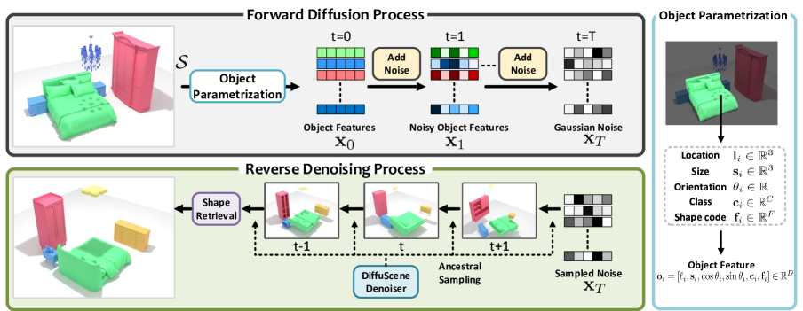
Figure 2: Overview. Given a 3D scene $\mathcal{S}$ of $N$ objects, we obtain its fully-connected scene graph $\vec{x}_{0}=\{\vec{o}_{i}\}_{i=1}^{N}$, by parametrizing each object $\vec{o}_{i}$ as a graph node storing all object attributes i.e., location $\vec{l}_{i}$, size $\vec{s}_{i}$, orientation $\theta_{i}$, class label $\vec{c}_{i}$, and latent shape code $\vec{f}_{i}$. Based on a set of all possible $\vec{x}_{0}$, we propose DiffuScene, a denoising diffusion probabilistic model for 3D scene graph generation. In the forward process, we gradually add noise to $\vec{x}_{0}$ until we obtain a standard Gaussian noise $\vec{x}_{T}$. In the reverse process i.e. generative process, a denoising network iteratively cleans the noisy graph using ancestral sampling. Finally, we use the denoised object features to perform shape retrieval for realistic scene synthesis.

2 Related work

Traditional Scene Modeling and Synthesis

Traditional methods usually formulate this problem into a data-driven optimization task, which consists of three key modules: scene formulation, prior representation, and optimization strategy. To extract the spatial relationship between objects, many approaches formulate objects in a scene as a graph [3, 4, 46, 85], and connect them with human bodies to build a human-centric graph [14, 17, 33, 46, 40]. To synthesize plausible 3D scene graphs, prior knowledge of reasonable scenes is required to drive scene optimization. Traditional scene priors are often inferred by following guidelines of interior design [35, 77], object frequency distributions (e.g., co-occurrence map of object categories) [3, 4, 12], affordance maps from human motions [14, 17, 27], scene arrangement examples [13, 17]. Constrained by scene priors, a new scene can be sampled with the above graph formulation using different optimization methods, e.g., iterative methods [14, 17], non-linear optimization [3, 46, 72, 77, 79, 13], or manual interaction [4, 35, 54]. Different from them, we adopt scene graph representation to learn complicated scene composition patterns from datasets, avoiding human-defined constraints and iterative optimization processes.

Learning-based Generative Scene Synthesis

3D deep learning reforms this task by learning scene priors in a fully automatic, end-to-end, and differentiable manner. The capacity to process large-scale datasets dramatically increases the inference ability in synthesizing diverse and reasonable object arrangements. Existing generative models for 3D scene synthesis are usually based on feed-forward networks [83], VAEs [44, 73] , GANs [74], Autoregressive models [42, 39, 68]. GAN methods produce high-quality results with fast sampling however, they often suffer from poor mode coverage and limited diversity. VAEs show better mode coverage but struggle to generate faithful samples [71]. Recurrent networks [30, 42, 39, 50, 66, 67, 68] including autoregressive models predict each new object conditioned on the previously generated objects. Thus, they are still limited by capturing complicated spatial relationships between objects. In contrast, we formulate scene generation as a scene graph diffusion process. A scene configuration is learned by denoising a set of noisy vectors with random object properties defined on graph nodes, which explicitly encodes diverse scene configuration modes into the denoising process and presents faithful object configurations.

3D Diffusion Models

After the pioneering work by [55] on using the diffusion process for data distribution learning, diffusion models [57, 58, 56, 22] have shown impressive visual quality in generative tasks, especially in various applications of 2D image synthesis, including image inpainting [34], super-resolution [53, 23], editing [34, 1], text-to-image synthesis [38, 51, 28], and video generation [25, 75]. Unlike 2D applications, diffusion models in the 3D domain receive much less attention, especially in 3D scenes. Most existing works focus on single object generation [32, 81, 84, 26, 82, 43]. In contrast to single objects, 3D scene synthesis shows much higher semantics and geometry complexity and a larger spatial extent. A concurrent work of LegoNet [80] uses a diffusion model to rearrange indoor furnitures into reasonable placements. However, it requires users to provide an initial scene with known furniture categories and shapes. Our method can support unconditional generation by synthesizing all 3D object properties characterized by their class categories, oriented 3D bounding boxes, and geometry features. In addition to scene re-arrangements, our method can be applied to scene completion and text-to-scene synthesis while LegoNet cannot.

3 DiffuScene

We introduce DiffuScene a scene graph denoising diffusion probabilistic model aiming at learning the distribution of 3D indoor scenes which includes semantic classes, surface geometries, and placements of multiple objects.

Specifically, we assume indoor scenes which are located in a world coordinate system whose origin is at the floor center, and that each scene $\mathcal{S}$ is a composition of at most $N$ objects $\{\vec{o}\}_{i=1}^{N}$. We represent such scenes by a fully-connected scene graph with $N$ graph nodes, where each node denotes an object.Each graph node (i.e. object) is defined by its class semantics $\vec{c}\in\mathbb{R}^{C}$, axis-aligned 3D bounding box size $\vec{s}\in\mathbb{R}^{3}$, location $\vec{\ell}\in\mathbb{R}^{3}$, rotation angle around the vertical axis $\vec{\theta}\in\mathbb{R}$, and shape code $\vec{f}\in\mathbb{R}^{F}$ extracted from object surfaces in the canonicalization system through a pre-trained shape auto-encoder [76]. Since the number of objects varies across different scenes, we define an additional ‘empty’ object and pad it into scenes to have a fixed number of objects across scenes. As proposed in [78], we represent the object rotation angle by parametrizing a 2-d vector of cosine and sine values. In summary, each object $\vec{o}_{i}$ is characterized by the concatenation of all attributes, i.e. $\vec{o}_{i}=[\vec{\ell}_{i},\vec{s}_{i},\cos\vec{\theta}_{i},\sin\vec{\theta}_{i},\vec{c}_{i},\vec{f}_{i}]\in\mathbb{R}^{D}$, where $D$ is the dimension of concatenated attributes.

Based on this graph representation, we define our denoising diffusion probabilistic model (Sec. 3.1), and propose different downstream applications like scene completion, scene re-arrangement, and text-conditioned scene synthesis in Sec. 3.2.

3.1 3D Scene Graph Diffusion

In Fig. 2 we shown an overview of our approach. We design a scene graph denoising probabilistic diffusion model where a series of Gaussian noise corruptions and removals on graph nodes perform the transitions between the noisy and the clean scene graph distributions.

Diffusion process.

The (forward) diffusion process is a pre-defined discrete-time Markov chain in the data space $\mathcal{X}$ spanning all possible scene graphs represented as 2D tensors of fixed size $\vec{x}\in\mathbb{R}^{N\times D}$, which are the concatenations of $N$ object properties $\{\vec{o}_{i}\}_{i=1}^{N}$ within a scene $\mathcal{S}$. Given a clean scene graph $\vec{x}_{0}$ from the underlying distribution $q(\vec{x}_{0})$, we gradually add Guassian noise to $\vec{x}_{0}$, obtaining a series of intermediate scene graph variables $\vec{x}_{1},...,\vec{x}_{T}$ with the same dimensionality as $\vec{x}_{0}$, according to a pre-defined, linearly increased noise variance schedule $\beta_{1},...,\beta_{T}$ (where $\beta_{1}<...<\beta_{T}$). The joint distribution $q(\vec{x}_{1:T}|\vec{x}_{0})$ of the diffusion process can be expressed as:

$$q(\vec{x}_{1:T}|\vec{x}_{0}):=\prod_{t=1}^{T}q(\vec{x}_{t}|\vec{x}_{t-1}),$$ (1)

where the diffusion step at time $t$ is defined as:

$$q(\vec{x}_{t}|\vec{x}_{t-1}):=\mathcal{N}(\vec{x}_{t};\sqrt{1-\beta_{t}}\vec{x}_{t-1},\beta_{t}\vec{I}).$$ (2)

A helpful property of diffusion processes is that we can directly sample $\vec{x}_{t}$ from $\vec{x}_{0}$ via the conditional distribution:

$$q(\vec{x}_{t}|\vec{x}_{0}):=\mathcal{N}(\vec{x}_{t};\sqrt{\bar{\alpha_{t}}}\vec{x}_{0},(1-\bar{\alpha_{t}})\vec{I}),$$ (3)

where $\vec{x}_{t}=\sqrt{\bar{\alpha}_{t}}\vec{x}_{0}+\sqrt{1-\bar{\alpha}_{t}}\vec{\epsilon}$ where $\alpha_{t}:=1-\beta_{t}$ , $\bar{\alpha}_{t}:=\prod_{r=1}^{t}\alpha_{s}$, and $\vec{\epsilon}$ is the noise used to corrupt $\vec{x}_{t}$.

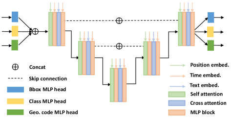
Figure 3: The denoising network architecture takes the graph nodes attributes (bounding box, object class, geometry code) as input and denoises them based on MLPs with skip connections and attention blocks.

Generative process.

The generative (i.e. denoising) process is parameterized as a Markov chain of learnable reverse Gaussian transitions. Given a noisy scene graph from a standard multivariate Gaussian distribution $\vec{x}_{T}\sim\mathcal{N}(\mathbf{0},\vec{I})$ as the initial state, it corrects $\vec{x}_{t}$ to obtain a cleaner version $\vec{x}_{t-1}$ at each time step by using a learned Gaussian transition $p_{\vec{\phi}}(\vec{x}_{t-1}|\vec{x}_{t})$ which is parameterized by a learnable network $\vec{\phi}$. By repeating this reverse process until the maximum number of steps $T$, we can reach the final state $\vec{x}_{0}$, the clean scene graph we aim to obtain. Specifically, the joint distribution of the generative process $p_{\vec{\phi}}(\vec{x}_{0:T})$ is formulated as:

$$p_{\vec{\phi}}(\vec{x}_{0:T}):=p(\vec{X}_{T})\prod_{t=1}^{T}p_{\vec{\phi}}(\vec{x}_{t-1}|\vec{x}_{t})$$ (4)

$$p_{\vec{\phi}}(\vec{x}_{t-1}|\vec{x}_{t}):=\mathcal{N}(\vec{x}_{t-1};\vec{\mu}_{\vec{\phi}}(\vec{x}_{t},t),\vec{\Sigma}_{\vec{\phi}}(\vec{x}_{t},t),),$$ (5)

where $\vec{\mu_{\phi}}(\vec{x}_{t})$ and $\vec{\Sigma}_{\vec{\phi}}(\vec{x}_{t})$ are the predicted mean and covariance, respectively, of the Gaussian $\vec{x}_{t-1}$ by feeding $\vec{x}_{t}$ into the denoising network $\vec{\phi}$. For simplicity, we take pre-defined constants for $\Sigma_{\vec{\phi}}(\vec{x}_{t}):=\sigma_{t}:=\frac{1-\bar{\alpha}_{t-1}}{1-\bar{\alpha}_{t}}\beta_{t}$, although Song et al. has shown that learnable covariances can increase generation quality in DDIM [58]. Ho et al. empirically found in DDPM [22] that rather than directly predicting $\vec{\mu}_{\vec{\phi}}(\vec{x}_{t},t)$, we can synthesize more high-frequent details by estimating the noise $\vec{\epsilon}_{\vec{\phi}}(\vec{x}_{t},t)$ applied to perturb $\vec{x}_{t}$. Then $\vec{\mu}_{\vec{\phi}}(\vec{x}_{t})$ can be re-parametrized by subtracting the predicted noise according to Bayes’s theorem:

$$\vec{\mu}_{\vec{\phi}}(\vec{x}_{t},t):=\frac{1}{\sqrt{\alpha_{t}}}(\vec{x}_{t}-\frac{\beta_{t}}{\sqrt{1-\bar{\alpha}_{t}}}\vec{\epsilon}_{\vec{\phi}}(\vec{x}_{t},t))$$ (6)

Denoising network.

As shown in Fig. 3, the denoiser in our method is based on MLPs with skip connections, where MLP blocks are interleaved with attention blocks [65] to aggregate the features of different objects, capturing the global context of a scene. As MLPs are shared with each object, it would be difficult for the denoising network to distinguish different objects without position information. To this end, we also use the positional embeddings of instance IDs and inject them into the network to guide the denoising process.

Training objective.

The goal of training the reverse diffusion process is to find optimal denoising network parameters $\vec{\phi}$ that can generate natural and plausible scenes. Our training objective is composed of two parts: i) A loss $L_{\text{sce}}$ to constrain that the generated scene graphs can approximate the underlying data distribution, and ii) a regularization term $L_{\text{iou}}$ to penalize the object intersections. The $L_{\text{sce}}$ is derived by maximizing the negative log-likelihood of the last denoised scene $\mathbb{E}[-\log p_{\vec{\phi}}(\vec{x}_{0})]$, which is yet not intractable to optimize directly. Thus, we can instead choose to maximize its variational upper bound:

$$L_{\text{sce}}:=\mathbb{E}_{q}[-\log\frac{p_{\phi}(\vec{x}_{0:T})}{q(\vec{x}_{1:T}|\vec{x}_{0})}]\geq\mathbb{E}[-\log p_{\vec{\phi}}(\vec{x}_{0})].$$ (7)

By surrogating variables, we can further simplify $L_{\text{sce}}$ as the sum of KL divergence between posterior $p_{\vec{\phi}}(\vec{x}_{t-1}|\vec{x}_{t},\vec{x}_{0})$ and conditional distribution $q(\vec{x}_{t}|\vec{x}_{t-1})$ at each $t$ :

$$L_{\text{sce}}:=\mathbb{E}_{q}[-\log p(\vec{x}_{T})-\sum_{t=1}^{T}\log\frac{p_{\vec{\phi}}(\vec{x}_{t-1}|\vec{x}_{t},\vec{x}_{0})}{q(\vec{x}_{t}|\vec{x}_{t-1})}],$$ (8)

where $-\log p(\vec{x}_{T})$ is a fixed constant since $\vec{x}_{T}\sim\mathcal{N}(0,\vec{I})$. Here, we refer the reader to DDPM [22] for the details of the derivation process. Moreover, we can re-write $L_{\text{sce}}$ into a simple and intuitive version that constrains the correct prediction of the corrupted noise on $\vec{x}_{t}$:

$$L_{\text{sce}}:=\mathbb{E}_{\vec{x}_{0},\vec{\epsilon},t}[\|\vec{\epsilon}-\vec{\epsilon}_{\vec{\phi}}(\vec{x}_{t},t)\|^{2}]$$ (9)

$$:=\mathbb{E}_{\vec{\phi}}[\|\vec{\epsilon}-\vec{\epsilon}_{\vec{\phi}}(\sqrt{\bar{\alpha}_{t}}\vec{x}_{0}+\sqrt{1-\bar{\alpha}_{t}}\vec{\epsilon},t)\|^{2}].$$

Based on Eq. 6, we can obtain the approximation of clean scene graph $\tilde{\vec{x}}_{0}^{t}$. Thus, we can compute $L_{\text{iou}}$ as the IoU summation of arbitrary two bounding boxes:

$$L_{\text{iou}}:=\sum_{t=1}^{T}\omega_{t}*\sum_{\vec{o}_{i},\vec{o}_{j}\in\tilde{\vec{x}}_{0}^{t}}\operatorname{IoU}(\vec{o}_{i},\vec{o}_{j}),$$ (10)

where the hyperparamter $\omega_{t}$ is set to $\bar{\alpha}_{t}*0.1$.

3.2 Applications

Based on the formulation of scene graph denoising diffusion probabilistic models in Sec. 3.1, we can further develop the model to support various downstream tasks with few modifications as shown in Fig. 1.

Scene completion.

Assuming a partial scene containing $M\leq N$ objects as $\vec{y}_{0}\in\mathbb{R}^{M\times D}$, we can utilize the learned scene priors from diffusion models to complement novel graph nodes $\hat{\vec{x}}_{0})$ into $\vec{y}_{0}$ to obtain a complete graph $\vec{x}_{0}=(\vec{y}_{0},\hat{\vec{x}}_{0})$. Similar to image in-painting [31, 51] and shape completion [32, 84, 81, 26, 82], the completion denoising process is almost same as the unconditional scene generation, except that we keep the already known graph nodes in the forward Guassian transitions $q$, and only hallucinate the missing ones through learnable reverse Guassian transitions $q_{\vec{\phi}}$. Concretely, the intermediate scene graphs during the diffusion process can be revised as $\vec{x}_{t}=(\vec{y}_{t},\hat{\vec{x}}_{t})$, where the partial scene graph $\vec{y}_{t}$ at time step $t$ is obtained by the forward diffusions. The completed scene graph $\hat{\vec{x}}_{t}$ is generated by the denoising process:

$$q(\vec{y}_{t}|\vec{y}_{t-1}):=\mathcal{N}(\vec{y}_{t};\sqrt{\bar{\alpha}_{t}}\vec{y_{0}},(1-\bar{\alpha}_{t}\vec{I})),$$ (11)

$$p_{\vec{\phi}}(\hat{\vec{x}}_{t-1}|\hat{\vec{x}}_{t}):=\mathcal{N}(\mu_{\vec{\phi}}(\vec{x}_{t},t),\sigma_{t}^{2}\vec{I}).$$

Scene re-arrangement.

Given a collection of objects with their surface geometries and semantics, we can leverage priors of the scene graph diffusion generative model to determine reasonable object placements by estimating their locations and orientations. Let us denote the noisy scene graph initialization as $\hat{\vec{x}}_{0}=[\hat{\vec{u}}_{0},\vec{v}]$, where $\hat{\vec{u}}_{0}=\{[\vec{l}_{i},\cos\theta_{i},\sin\theta_{i}]\}_{i=1}^{N}$ is the concatenation of $N$ objects’ locations and orientations, and $\vec{v}=\{[\vec{s}_{i},\vec{c}_{i},\vec{f}]\}_{i=1}^{N}$ is the concatenation of $N$ objects’ sizes, category classes, and shape codes. The intermediate scenes during the arrangement diffusion process can be expressed as:

$$p_{\vec{\phi}}(\hat{\vec{u}}_{t-1}|\hat{\vec{u}}_{t}):=\mathcal{N}(\mu_{\vec{\phi}}(\hat{\vec{u}}_{t},t,\vec{v}),\sigma_{t}^{2}\vec{I}),$$ (12)

where we iteratively update the object locations and orientations $\vec{u}_{t}$ via $p_{\vec{\phi}}$ conditioned on $\vec{v}$.

Text-conditioned scene synthesis.

Given a list of sentences describing the desired object classes and inter-object spatial relationship as conditional inputs, we can employ a pre-trained BERT encoder [9] to extract word embeddings $\vec{z}\in\mathbb{R}^{48\times 768}$, then we utilize cross attention layers to inject the language guidance into the denoising network that predicts out noise via $\vec{\epsilon}_{\vec{\phi}}(\vec{x}_{t},t,\vec{z})$, as depicted in Fig. 3.

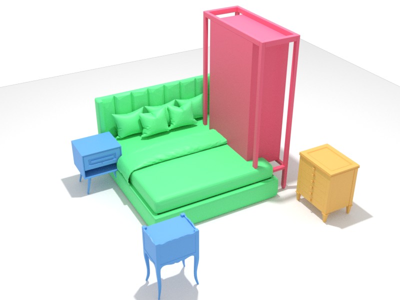
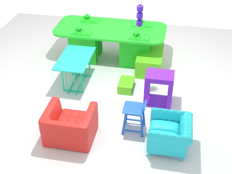
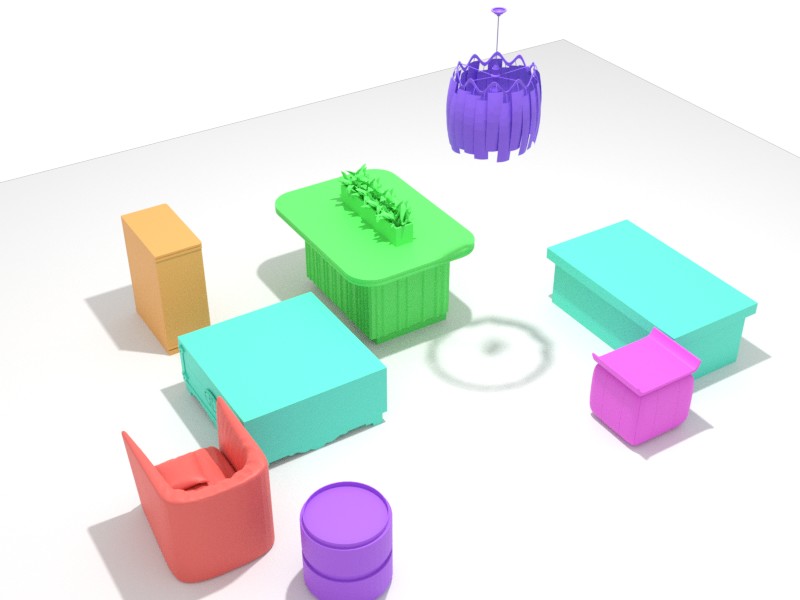
(a) DepthGAN [74]

         

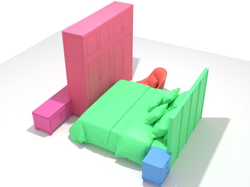
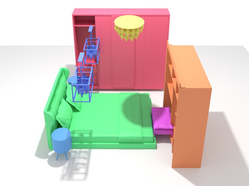
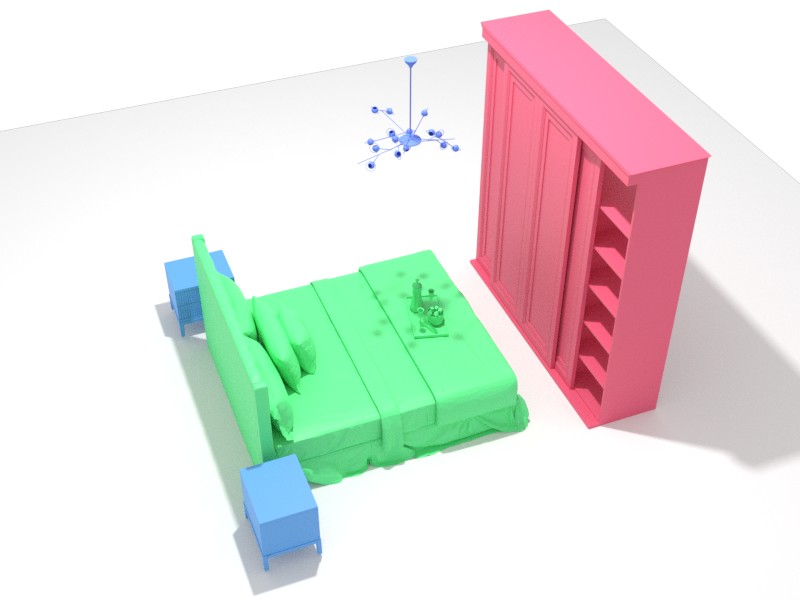
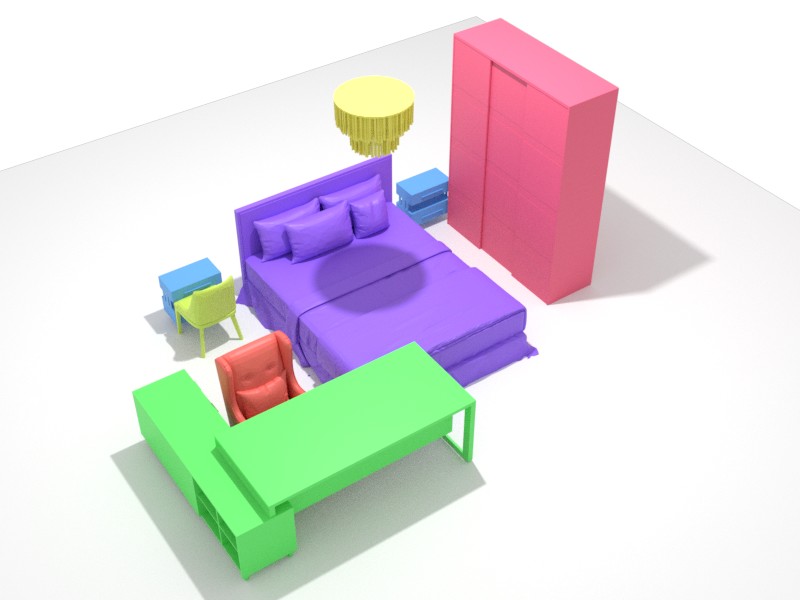
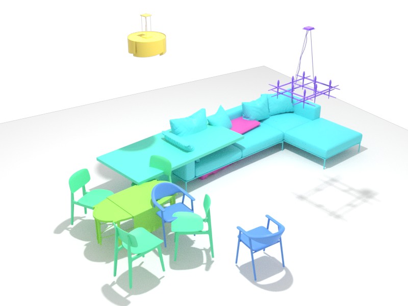
(b) Sync2Gen [73]

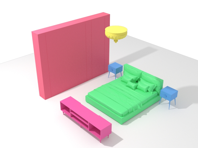
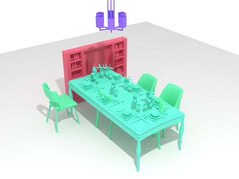
(c) ATISS [42]

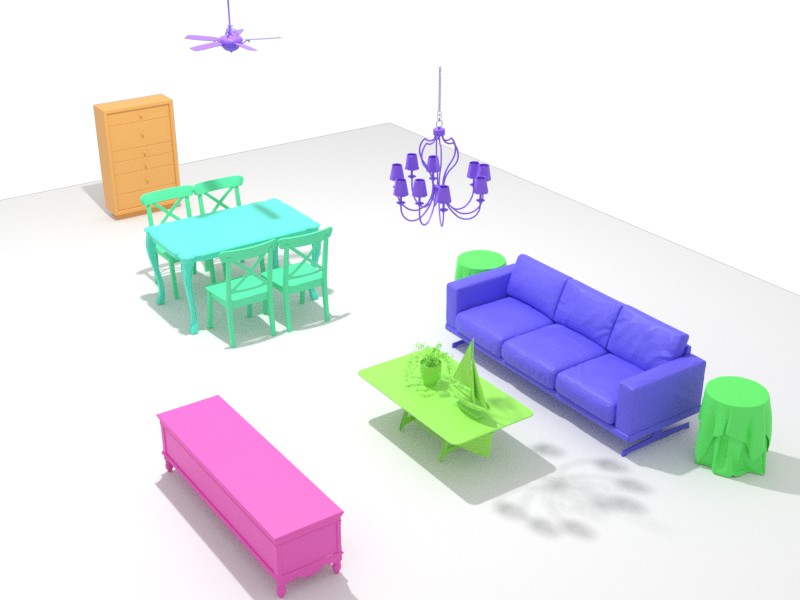
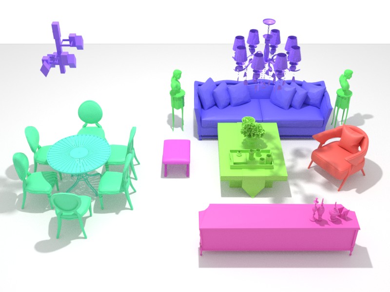
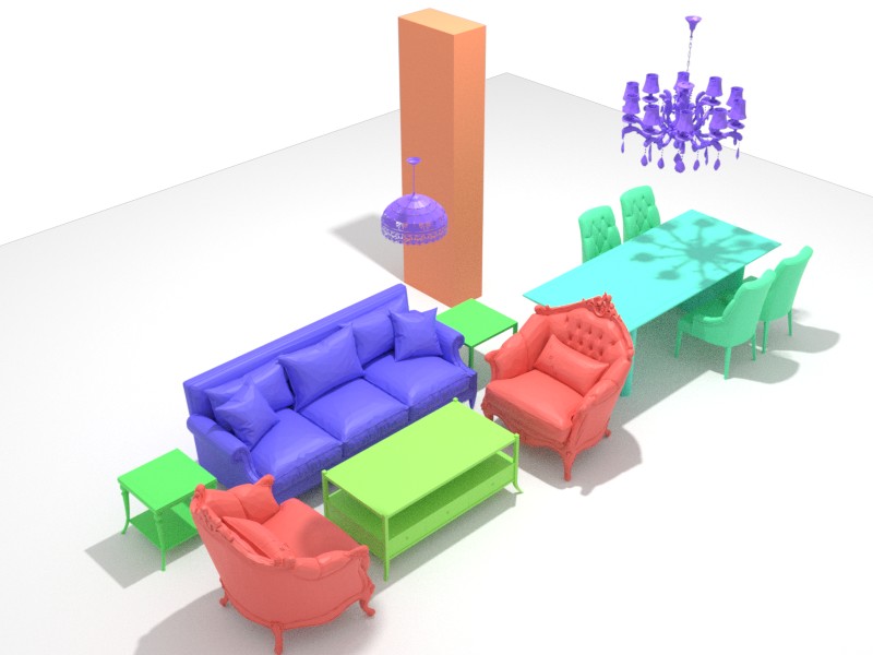
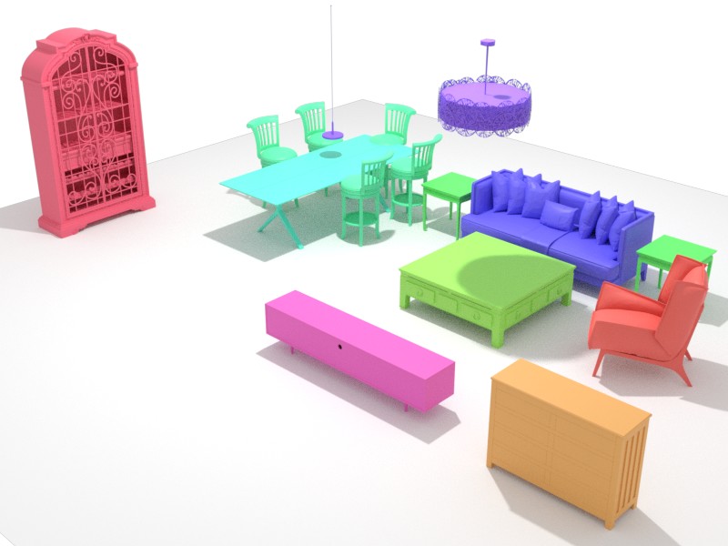
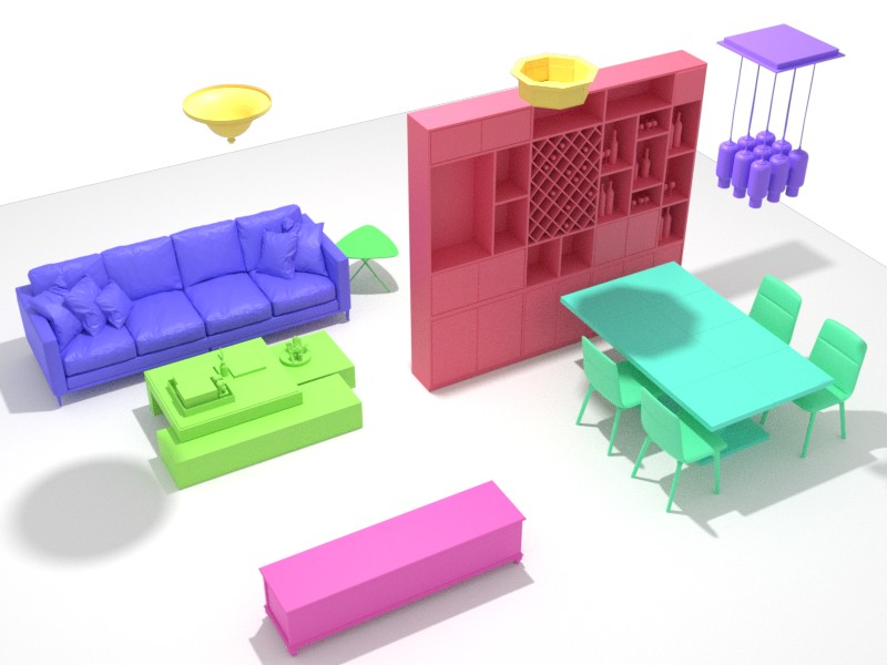
(d) Ours

Figure 4: Unconditional scene synthesis. We compare our method with the state-of-the-art by generating from random noises, where our results present higher diversity and better plausibility with fewer penetration issues.

4 Experiments

Datasets

For experimental comparisons, we use the large-scale 3D indoor scene dataset 3D-FRONT [15] as the benchmark. 3D-FRONT is a synthetic dataset composed of 6,813 houses with 14,629 rooms, where each room is arranged by a collection of high-quality 3D furniture objects from the 3D-FUTURE dataset [16]. Following ATISS [42], we use three types of indoor rooms for training and evaluation, including 4,041 bedrooms, 900 dining rooms, and 813 living rooms. For each room type, we use $80\%$ of rooms as the training sets, while the remaining are for testing.

Baselines

We compare against state-of-the-art scene synthesis approaches using various generative models, including: 1) DepthGAN [74], learning a volumetric generative adversarial network from multi-view semantic-segmented depth maps; 2) Sync2Gen [73], learning a latent space through a variational auto-encoder of scene object arrangements represented by a sequence of 3D object attributes; A Bayesian optimization stage based on the relative attributes prior model further regularized and refined the results. 3) ATISS [42], an autoregressive model to sequentially predict the 3D object bounding box attributes.

Implementation

We train our scene diffusion models on different types of indoor rooms respectively. They are trained on a single RTX 3090 with a batch size of 128 for $T=100,000$ epochs. The learning rate is initialized to $lr={2}\mathrm{e}{-4}$ and then gradually decreases with the decay rate of 0.5 in every 15,000 epochs. For the diffusion processes, we use the default settings from the denoising diffusion probabilistic models (DDPM) [22], where the noise intensity is linearly increased from 0.0001 to 0.02 with 1,000-time steps. During inference, we first use the ancestral sampling strategy to obtain a scene graph and then retrieve the most similar CAD model in the 3D-FUTURE [16] for each object based on generated shape codes and sizes.

Method	Bedroom				Dining room				Living room
	FID $\downarrow$	KID $\downarrow$	SCA $\%$	CKL $\downarrow$	FID $\downarrow$	KID $\downarrow$	SCA $\%$	CKL $\downarrow$	FID $\downarrow$	KID $\downarrow$	SCA $\%$	CKL $\downarrow$
DepthGAN [74]	40.15	18.54	96.04	5.04	81.13	50.63	98.59	9.72	88.10	63.81	97.85	7.95
Sync2Gen*	33.59	13.78	87.11	2.67	48.79	12.01	91.43	5.03	47.14	11.42	86.71	1.60
Sync2Gen [73]	31.07	11.21	82.97	2.24	46.05	8.74	88.02	4.96	48.45	12.31	84.57	7.52
ATISS [42]	18.60	1.72	61.71	0.78	38.66	5.62	71.34	0.64	40.83	5.18	72.66	0.69
Ours	18.29	1.42	53.52	0.35	32.60	0.72	55.50	0.22	36.18	0.88	57.81	0.21

Table 1: Quantitative comparisons on the task of unconditional scene synthesis. The Sync2Gen* is a variant of Sync2Gen [73] without Bayesian optimization. Note that for the Scene Classification Accuracy (SCA), the score closer to $50\%$ is better.

Evaluation Metrics

Following previous works [68, 73, 42], we use Fréchet inception distance (FID ) [21], Kernel inception distance [2] (KID $\times$ 0.001), scene classification accuracy (SCA), and category KL divergence (CKL $\times$ 0.01) to measure the plausibility and diversity of 1,000 synthesized scenes. For FID, KID, and SCA, we render the generated and ground-truth scenes into 256$\times$256 semantic maps through top-down orthographic projections, where the texture of each object is uniquely determined by the associate color of its semantic class. We use a unified camera and rendering setting for all methods to ensure fair comparisons. For CKL, we calculate the KL divergence between the semantic class distributions of synthesized scenes and ground-truth scenes. For FID, KID, and CKL, the lower number denotes a better approximation of the data distribution. FID and KID can also manifest the result diversity. For the SCA, a score close to $50\%$ represents that the generated scenes are indistinguishable from real scenes.

4.1 Unconditional Scene Synthesis

Fig. 4 visualizes the qualitative comparisons of different scene synthesis methods. We observe that both DepthGAN [74] and Sync2Gen [73] are vulnerable to object intersections. While ATISS [42] can alleviate the penetration issue by autoregressive scene priors, it cannot always generate reasonable scene results. However, our scene graph diffusion can synthesize natural and diverse scene arrangements. Tab. 1 presents the quantitative comparisons under various evaluation metrics. Our method consistently outperforms others in all metrics, which clearly demonstrates that our method can generate more diverse and plausible scenes.

Method	FID $\downarrow$	KID $\downarrow$	SCA $\%$	CKL $\downarrow$
Ours-Grid-$8^{3}$	31.28	14.81	84.55	6.23
Ours-Plane-$32^{2}$	28.17	11.12	83.80	2.67
Ours-PVCNN	25.81	8.55	72.98	1.53
Ours-Transformer	29.08	4.59	73.63	0.36
Ours-Single head	19.78	2.07	54.53	0.69
Ours-w/o geometry code	18.40	1.55	55.42	0.66
Ours-final	18.29	1.42	53.52	0.35

Table 2: Quantitative ablation studies on the task of unconditional scene synthesis on the 3D-FRONT bedrooms.

Method	Bedroom			Dining room
	FID $\downarrow$	KID $\downarrow$	SCA $\%$	FID $\downarrow$	KID $\downarrow$	SCA $\%$
ATISS [42]	30.54	2.38	26.73	42.65	8.32	43.99
Ours	27.32	1.92	40.30	40.99	6.31	49.06

Table 3: Quantitative comparisons on the task of scene completion on the 3D-FRONT bedrooms and dining rooms. Only 3 objects are given in the partial scenes.

We conduct detailed ablation studies to verify the effectiveness of each design in our scene graph diffusion models. The quantitative results are provided in Tab. 2.

What is the effect of scene graphs?

Instead of using scene graphs, we can store object properties in regular 2D plane images or 3D volumetric grids. Then, we can use conventional 2D U-Net or 3D U-Net [52] with attention layers to learn the diffusion object properties. However, the performances are inferior to our proposed scene graph diffusion.

What is the effect of MLP+Attention as the denoiser?

We investigate the different choices of denoising networks. The performances degrade when we use the Point-Voxel CNN [84] or the transformer in DALLE-2 [47].

The effect of multiple prediction heads in the denoiser.

In the denoiser, we use three different encoding and prediction heads for respective object properties, e.g. bounding box parameters, semantic class labels, and geometry codes. We found that a single head to process and predict all attributes together is less effective than multiple heads.

What is the effect of geometry code diffusion?

With the geometry code diffusion, the model can acquire a more accurate and holistic understanding of indoor scenes, facilitating more realistic scene synthesis. This can be verified in the improvement of SCA. Besides, the decrease in CKL can manifest that the joint diffusion of geometry code and object layout can promote the model to learn more accurate object class distribution.

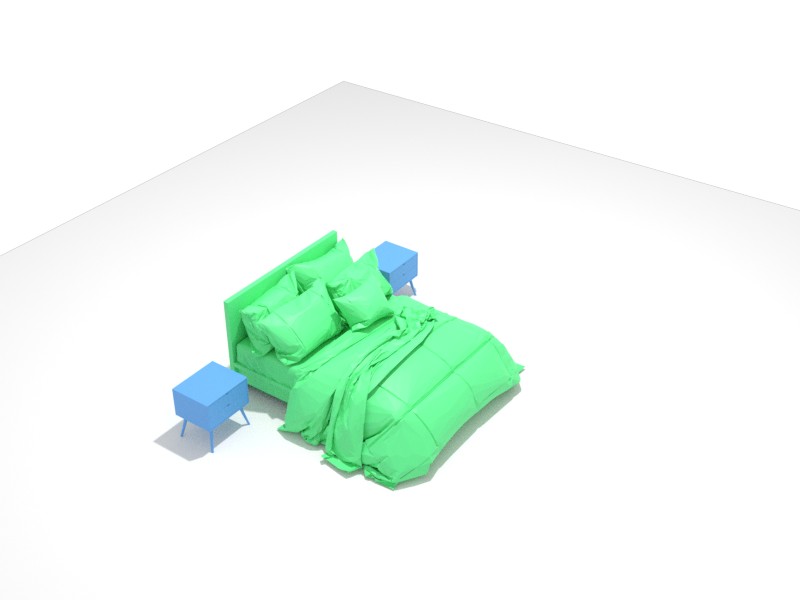
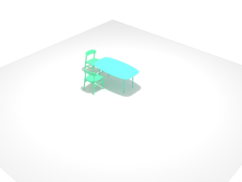
(a) Partial Scenes

     

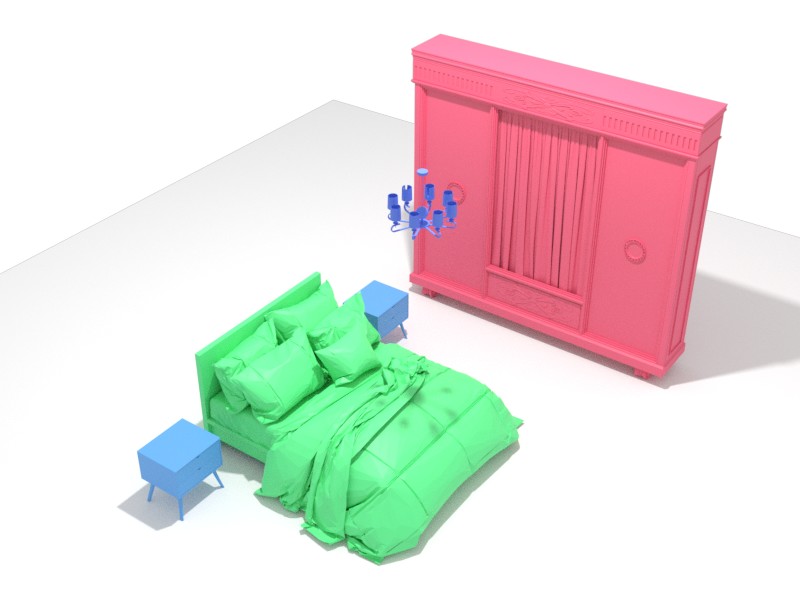
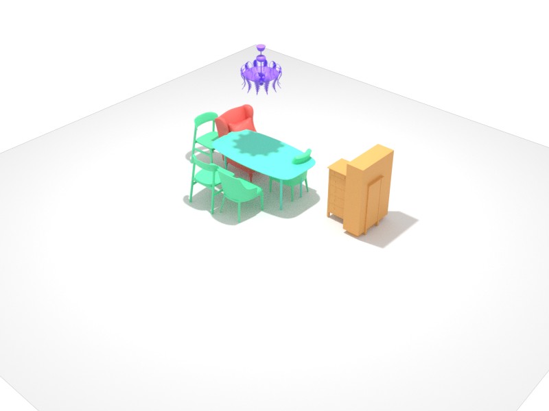
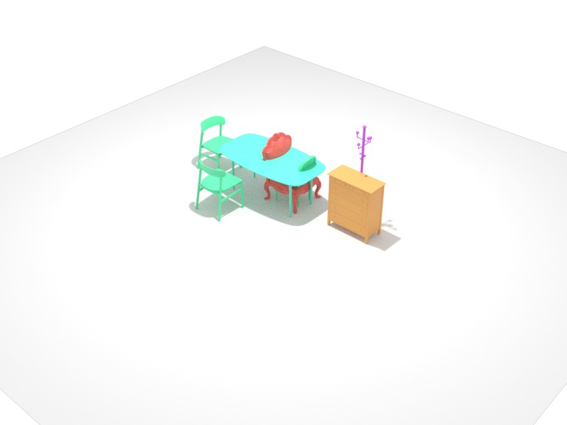
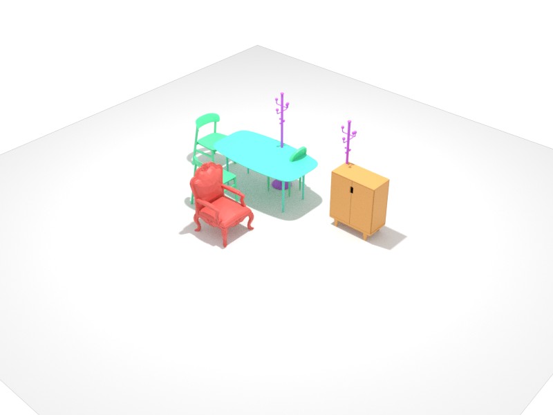
(b) ATISS [42]

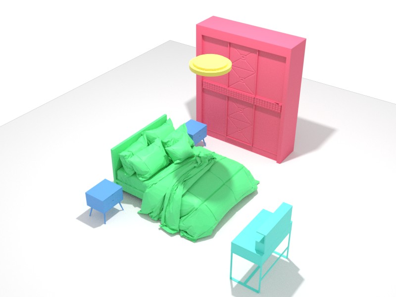
(c) Ours

Figure 5: Scene completion from partial scenes with only 3 objects given as inputs. Compared to ATISS, our diffusion-based method produced more diverse completion results with higher fidelity.

(a) Noisy Scenes

     

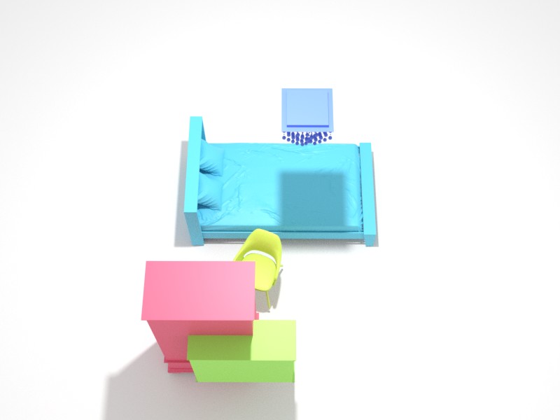
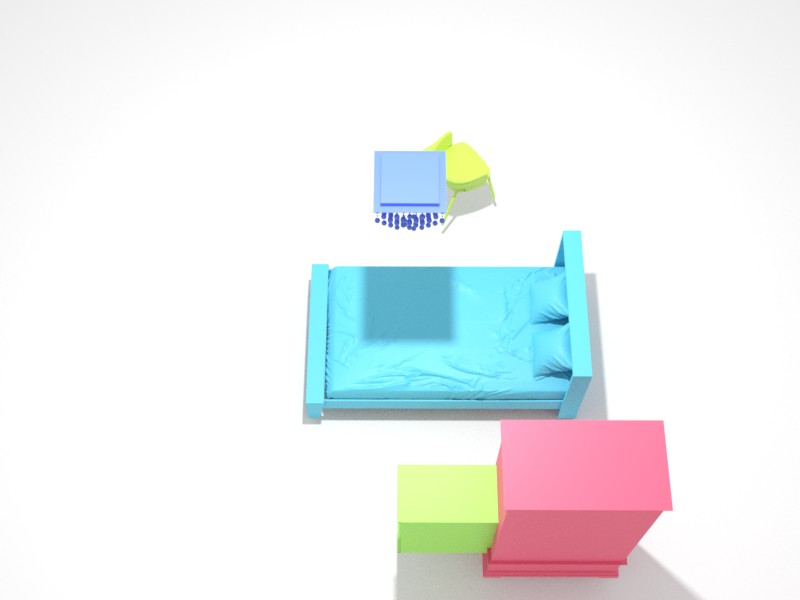
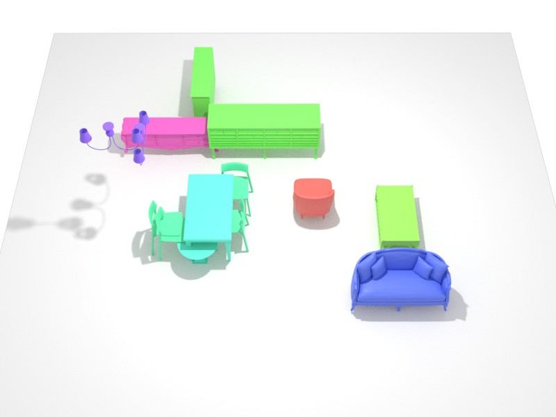
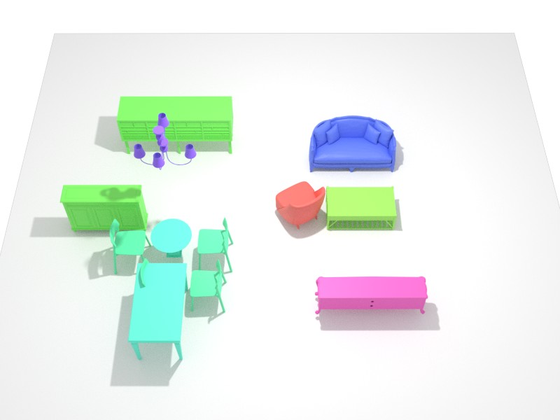
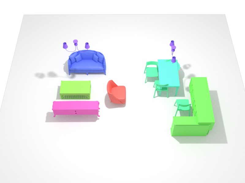
(b) ATISS [42]

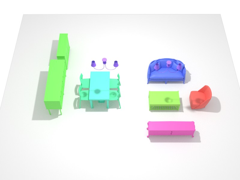
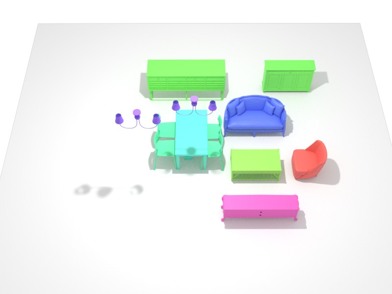
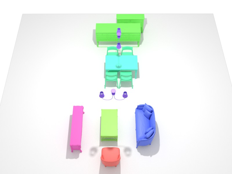
(c) Ours

Figure 6: Scene re-arrangements of collections of random objects. Compared to ATISS, our diffusion-based method generates various object placement options with better plausibility.

4.2 Applications

Scene Completion

We compare against ATISS [42] on the task of scene completion. As shown in Fig. 5, our method can produce more diverse completion results with high fidelity. This can also be verified by the quantitative comparisons in Tab. 3.

Scene Re-arrangement

We also conduct comparisons with ATISS [42] on the application of scene re-arrangement. As depicted in Fig. 6, our method is generating various object placements with better plausibility compared to ATISS.

Text-conditioned Scene Synthesis

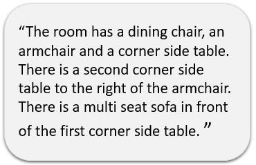
(a) Input text

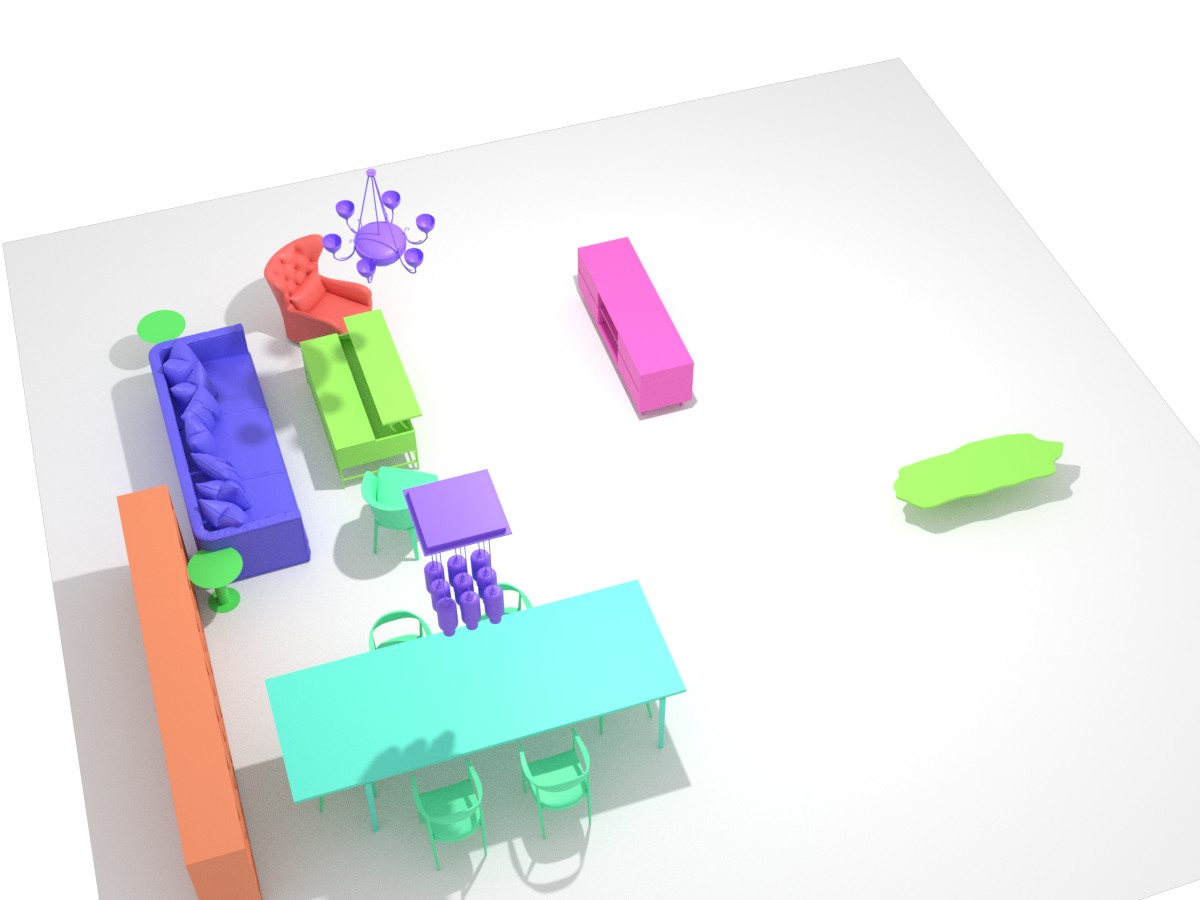
(b) Reference

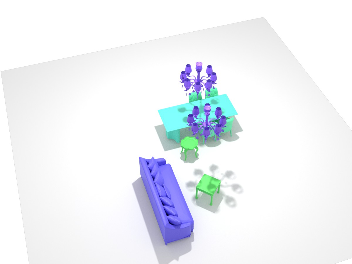
(c) ATISS [42]

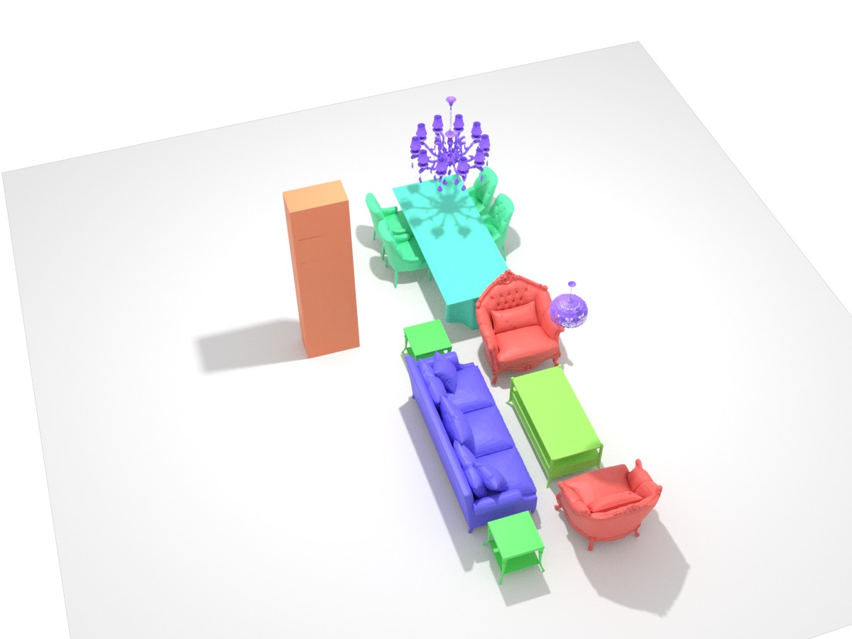
(d) Ours

Figure 7: Text-conditioned scene synthesis. The input text only describes a partial scene configuration. Our method generates a more plausible scene matched with the text.

Given a text prompt describing a partial scene configuration, we aim to synthesize a full scene satisfying the input. We conduct a perceptual user study for the text-conditioned scene synthesis. Given a text prompt and a ground-truth scene as a reference, we ask the attendance two questions for each pair of results from ATISS and ours: which of the synthesized scenes is closely matched with the input text, and which one is more realistic and reasonable. We collect the answers of 225 scenes from 45 users. Please refer to the supplementary material for the details of user study. 62$\%$ of users prefer our method to ATISS in realism. 55$\%$ of users are in favor of us in the matching score. This illustrates that our text-conditioned model generates more realistic scenes while capturing more accurate object relationships described in the text prompt.

4.3 Limitations

Although we have shown impressive scene synthesis results, there are still some limitations in our method. Firstly, we only consider single-room generation and train our model on a specific room type. Thus, our method cannot synthesize large-scale scenes with multiple rooms. Secondly, the object textures are from the provided 3D CAD model dataset via shape retrieval. An interesting direction is to integrate texture diffusion into our model. Lastly, we rely on 3D labeled scenes to drive the learning of scene diffusion. Leveraging scene datasets with only 2D labels to learn scene diffusion priors is also a promising direction. We leave these mentioned limitations as our future efforts.

5 Conclusion

In this work, we introduced DiffuScene, a novel method for generative indoor scene synthesis based on a scene graph denoising diffusion probabilistic model that learns holistic scene configuration priors in the joint diffusion process of object semantics, bounding boxes, and geometry features.We applied our method to several downstream applications, namely scene completion, scene re-arrangement, and text-conditioned scene synthesis. Compared to prior state-of-the-art methods our approach can synthesize more plausible and diverse indoor scenes as has been measured by different metrics and confirmed in a user study. Our method is an important piece in the puzzle of 3D generative modeling and we hope that it will inspire research in denoising diffusion-based 3D synthesis.

Acknowledgement.

This work is supported by a TUM-IAS Rudolf Mößbauer Fellowship, the ERC Starting Grant Scan2CAD (804724), and Sony Semiconductor Solutions.

In this supplemental material, we provide details for our implementation in Sec. A, dataset pre-processing and text prompt generation in Sec. B, baseline implementations in Sec. C, additional results in Sec. D, and user studies in Sec. E.

Appendix A Implementations

A.1 Shape Auto-Encoder

We adopt a pre-trained shape auto-encoder to extract a set of latent shape codes for CAD models from the 3D-FUTURE [16] dataset. The network architecture of the shape auto-encoder is shown in Fig. 8. It is a variational auto-encoder, similar to FoldingNet [76]. Specifically, a point cloud $\mathbf{P}_{in}$ of size 2,048 is fed into a graph encoder based on PointNet [45] with graph convolutions [69] to extract a global latent code of dimension 512, which is used to predict the mean $\mathbf{\mu}$ and variance $\mathbf{\sigma}$ of a low-dimensional latent space of size 64. Subsequently, a compressed latent is sampled from $\mathcal{N}(\mathbf{\mu},\mathbf{\sigma})$. Finally, the compressed latent is mapped back to the original space and passed to the FoldingNet decoder to recover a point cloud $\mathbf{P}_{rec}$ of size 2,025. The used training objective is a weighted combination of Chamfer distance (i.e. CD) and KL divergence.

$$L_{vae}=\operatorname{CD}(\mathbf{P}_{in},\mathbf{P}_{rec})+\omega_{kl}*\operatorname{KL}(\mathcal{N}(\mathbf{\mu},\mathbf{\sigma})||\mathcal{N}(\mathbf{0},\mathbf{I})),$$ (13)

where $\omega_{kl}$ is set to 0.001. The latent compression and KL regularization leads to a compact and structured latent space, focusing on global shape structures. The shape autoencoder is trained on a single RTX 2080 with a batch size of 16 for 1,000 epochs. The learning rate is initialized to $lr={1}\mathrm{e}{-4}$ and then gradually decreases with the decay rate of 0.1 in every 400 epochs.

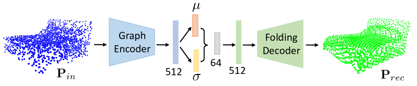
Figure 8: Shape Auto-encoder.

A.2 Shape Code Diffusion

We use the extracted latent codes to train shape code diffusion. While we apply KL regularization, the value range of latent codes is still unbound. To make it easier to diffuse, we scale the latent codes to $[-1,1]$ by using the statistical minimum and maximum feature values over the whole set. During inference, we rescale generated shape codes.

A.3 Shape Retrieval

During inference, we use shape retrieval as the post-processing procedure to acquire object surface geometries for generated scene graphs. Concretely, for each graph node, we perform the nearest neighbor search in the 3D-FUTURE [16] dataset to find the CAD model with the same class label, the closest bounding box size, and the closest geometry feature. Previous works [68, 42] only use object semantics and bounding box sizes during shape retrieval, we consider the similarity of geometry descriptors. Thus, our method can retrieve more accurate shape geometries. After the object retrieval, we place the retrieved CAD models into the scene based on the predicted locations, orientation angles, and sizes.

Appendix B Dataset

Preprocessing

The dataset preprocessing is based on the setting of ATISS [42]. We start by filtering out those scenes with problematic object arrangements such as severe object intersections or incorrect object class labels, e.g., beds are misclassified as wardrobes in some scenes. Then, we remove those scenes with unnatural sizes. The floor size of a natural room is within $6m\times 6m$ and its height is less than $4m$. Subsequently, we ignore scenes that have too few or many objects. The number of objects in valid bedrooms is between 3 and 13. As for dining and living rooms, the minimum and maximum numbers are set to 3 and 21 respectively. Thus, the number of scene graph nodes is $N=13$ in bedrooms and $N=21$ in dining and living rooms. In addition, we delete scenes that have objects out of pre-defined categories. After pre-processing, we obtained 4,041 bedrooms, 900 dining rooms, and 813 living rooms.

For the semantic class diffusion, we have an additional class of ‘empty’ to define the existence of an object. Combining with the object categories that appeared in each room type, we have $L=22$ object categories for bedrooms, and $L=25$ object categories for dining and living rooms in total. The category labels are listed as follows.

# 22 3D-Front bedroom categories [’empty’, ’armchair’, ’bookshelf’, ’cabinet’, ’ceiling_lamp’, ’chair’, ’children_cabinet’, ’coffee_table’, ’desk’, ’double_bed’, ’dressing_chair’, ’dressing_table’, ’kids_bed’, ’nightstand’, ’pendant_lamp’, ’shelf’, ’single_bed’, ’sofa’, ’stool’, ’table’, ’tv_stand’, ’wardrobe’]

# 25 3D-Front dining or living room categories [’empty’, ’armchair’, ’bookshelf’, ’cabinet’, ’ceiling_lamp’, ’chaise_longue_sofa’, ’chinese_chair’, ’coffee_table’, ’console_table’, ’corner_side_table’, ’desk’, ’dining_chair’, ’dining_table’, ’l_shaped_sofa’, ’lazy_sofa’, ’lounge_chair’, ’loveseat_sofa’, ’multi_seat_sofa’, ’pendant_lamp’, ’round_end_table’, ’shelf’, ’stool’, ’tv_stand’, ’wardrobe’, ’wine_cabinet’]

Text Prompt Generation

We follow the SceneFormer [68] to generate text prompts describing partial scene configurations. Each text prompt contains one to three sentences. We explain the details of text formulation process by using the text prompt ’The room has a dining table, a pendant lamp, and a lounge chair. The pendant lamp is above the dining table. There is a stool to the right of the lounge chair.‘ as an example. First, we randomly select three objects from a scene, get their class labels, and then count the number of appearances of each selected object category. As such, we can get the first sentence. Then, we find all valid object pairs associated with the selected three objects. An object pair is valid only if the distance between two objects is less than a certain threshold that is set to 1.5 in our method. Next, we calculate the relative orientations and translations, from which we can determine the relationship type of the valid object pair from the candidate pool: ’is above to‘, ’is next to‘, ’is left of‘, ’is right of‘, ’ surrounding‘, ’inside‘, ’behind‘, ’in front of‘, and ’on‘. In this way, we can acquire some relation-describing sentences like the second and third sentences in the example. Finally, we randomly sampled zero to two relation-describing sentences.

Appendix C Baselines

DepthGAN

DepthGAN [74] adopts a generative adversary network to train 3D scene synthesis using both semantic maps and depth images. The generator network is built with 3D convolution layers, which decode a volumetric scene with semantic labels. A differentiable projection layer is applied to project the semantic scene volume into depth images and semantic maps under different views, where a multi-view discriminator is designed to distinguish the synthesized views from ground-truth semantic maps and depth images during the adversarial training.

Sync2Gen

Sync2Gen [73] represents a scene arrangement as a sequence of 3D objects characterized by different attributes (e.g., bounding box, class category, shape code). The generative ability of their method relies on a variational auto-encoder network, where they learn objects’ relative attributes. Besides, a Bayesian optimization stage is used as a post-processing step to refine object arrangements based on the learned relative attribute priors.

ATISS

ATISS [42] considers a scene as an unordered set of objects and then designs a novel autoregressive transformer architecture to model the scene synthesis process. During training, based on the previously known object attributes, ATISS utilizes a permutation-invariant transformer to aggregate their features and predicts the location, size, orientation, and class category of the next possible object conditioned on the fused feature. The original version of ATISS [42] is conditioned on a 2D room mask from the top-down orthographic projection of the 3D floor plane of a scene. To ensure fair comparisons, we train an unconditional ATISS without using a 2D room mask as input, following the same training strategies and hyperparameters as the original ATISS.

Appendix D Additional Results

Unconditional Scene Synthesis

         

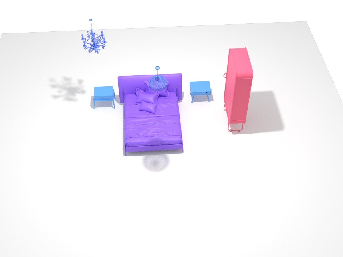
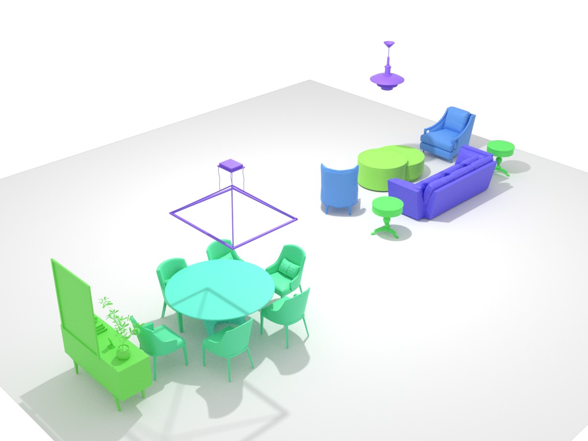
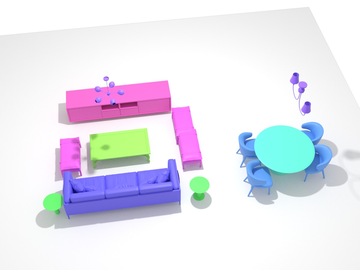
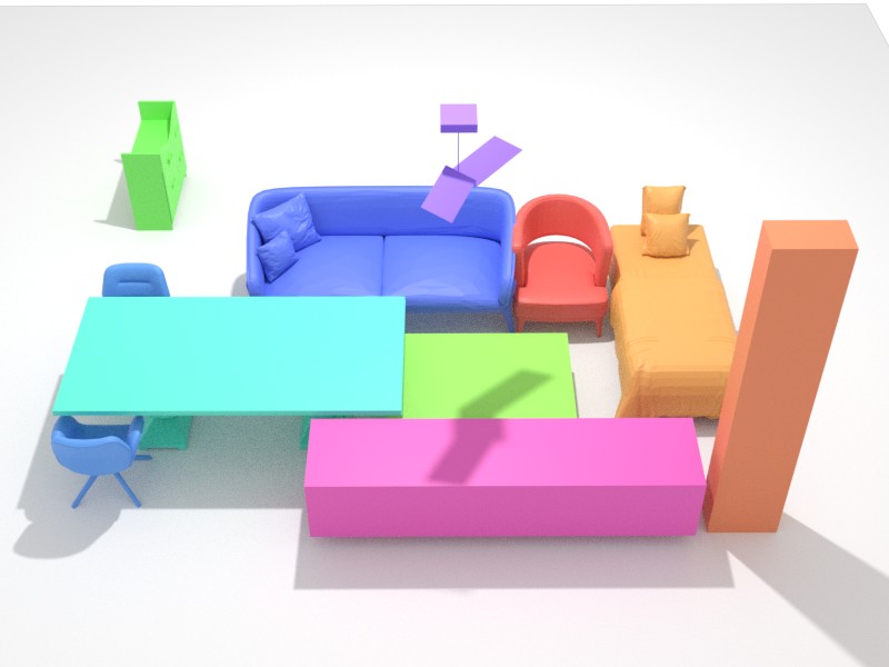
Figure 9: Diverse and plausible results of unconditional scene synthesis from our method.

In Fig. 9, we provide more visualization results of our unconditional scene synthesis model.

Scene Completion

(a) Partial Scenes

     

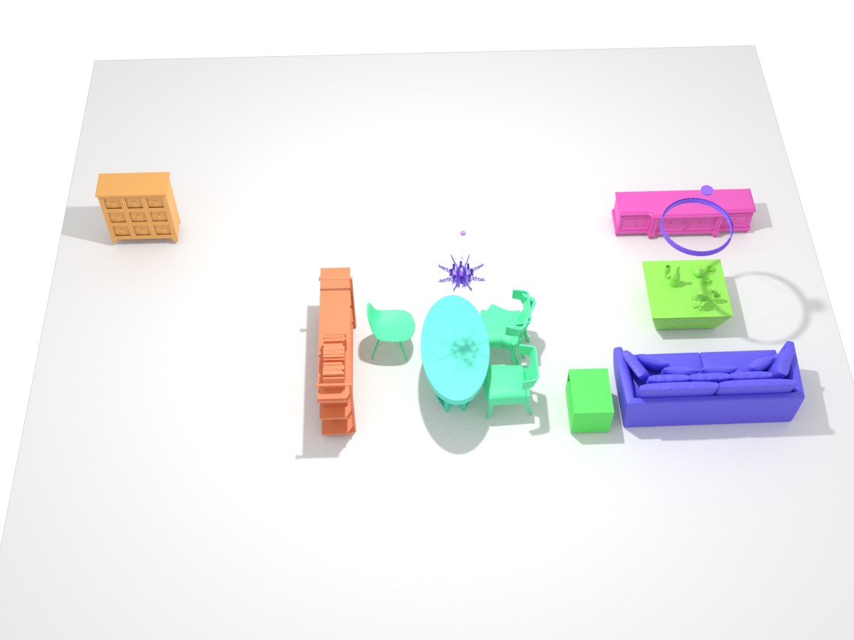
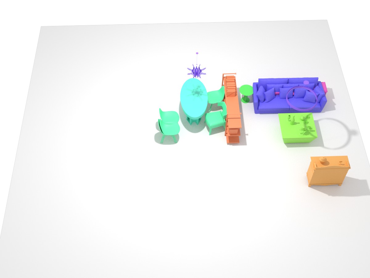
(b) ATISS [42]

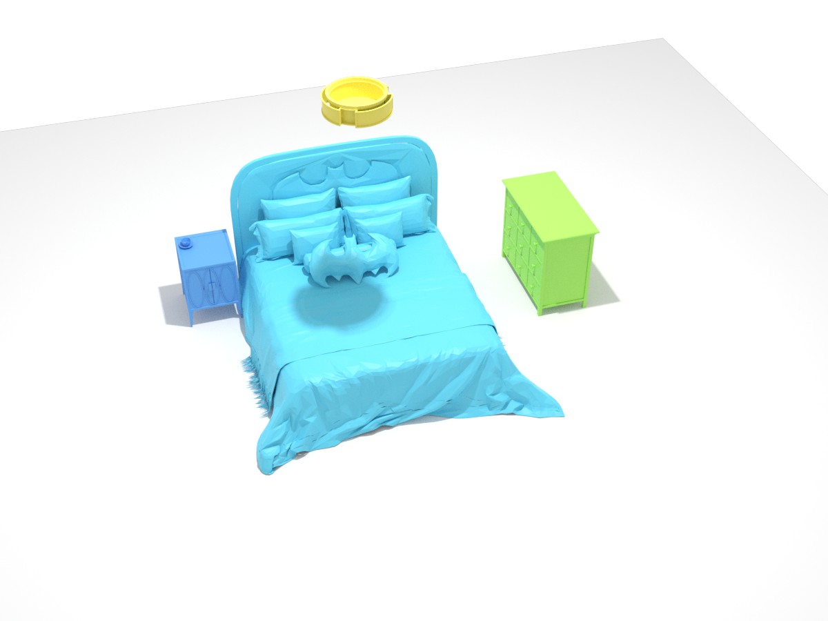
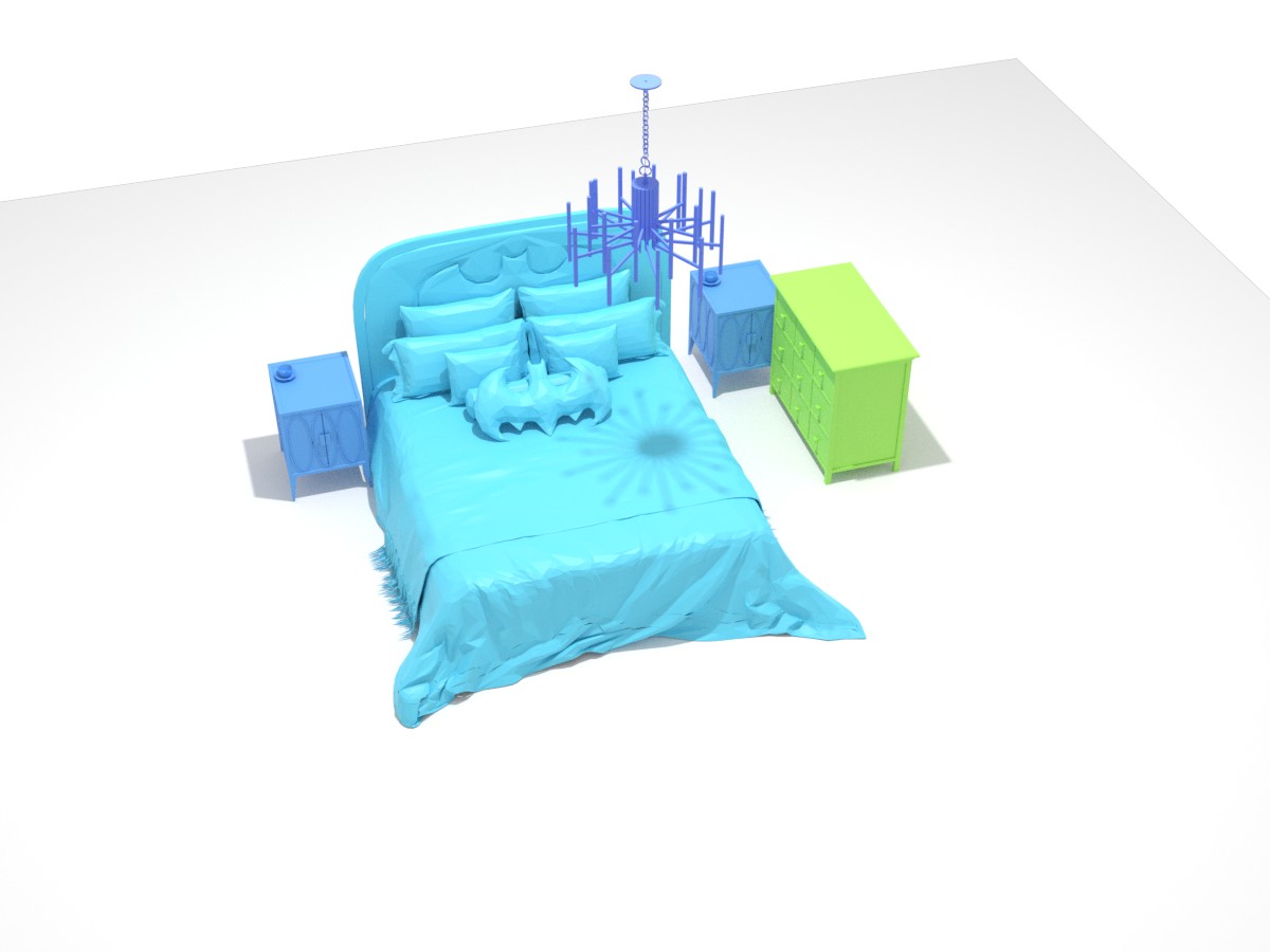
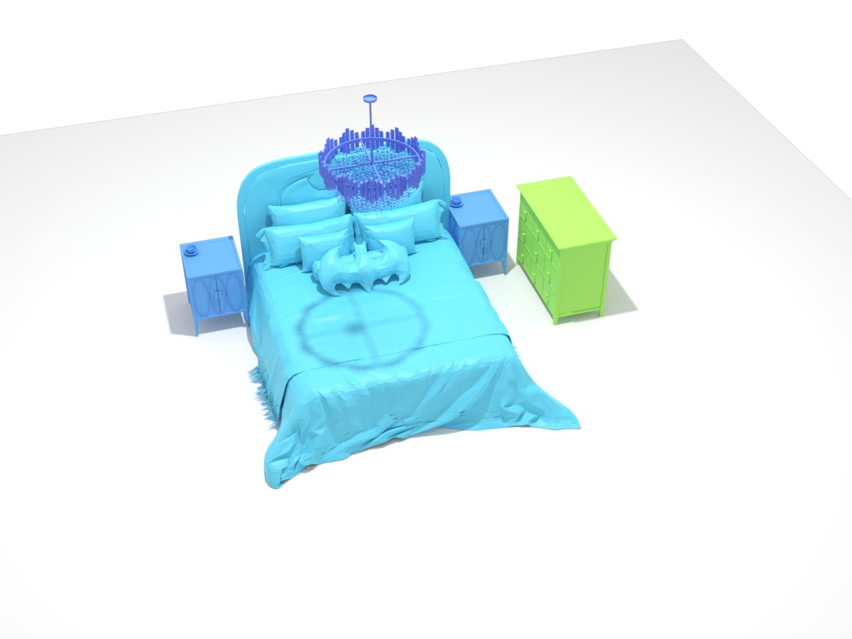
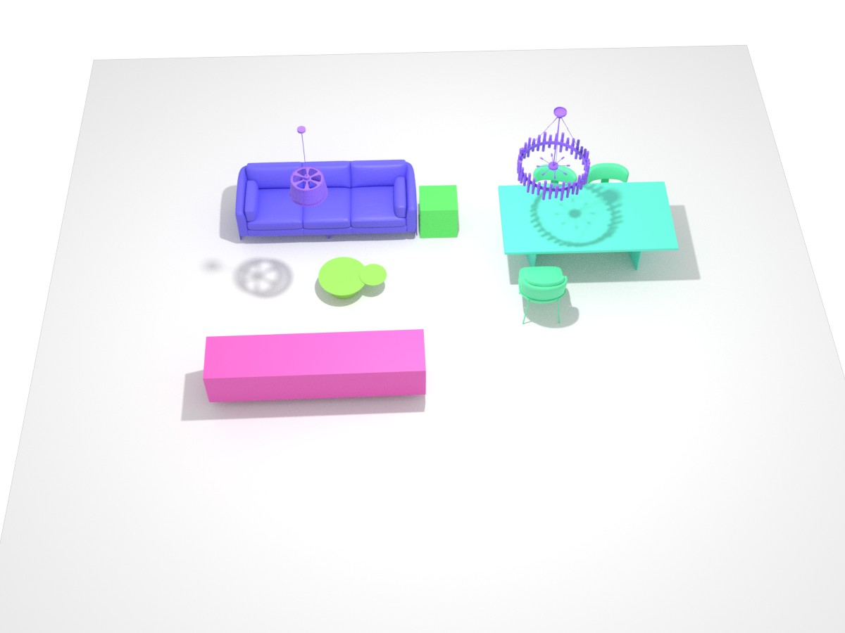
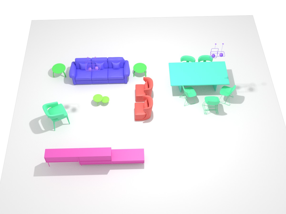
(c) Ours

Figure 10: Scene completion from partial scenes with only three objects given as inputs. Compared to ATISS, our method produced more diverse completion results with higher fidelity.

We present more qualitative comparisons on the task of scene completion in Fig. 10.

Scene Arrangement

(a) Noisy Scenes

     

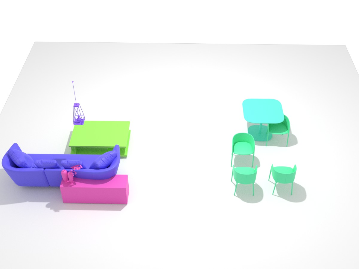
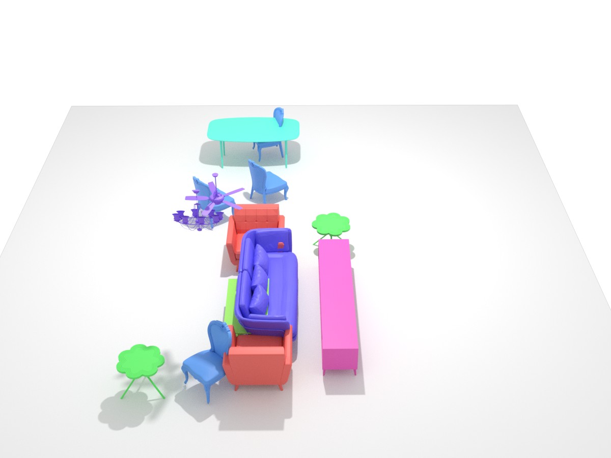
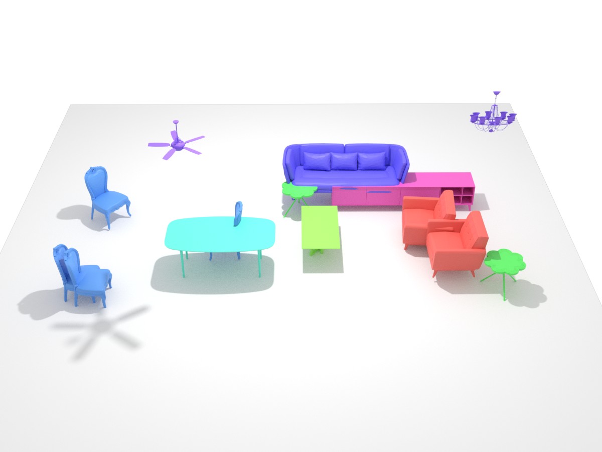
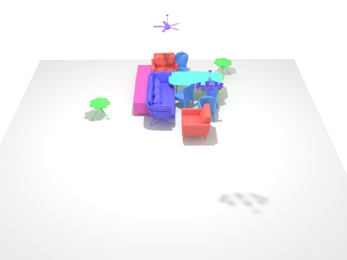
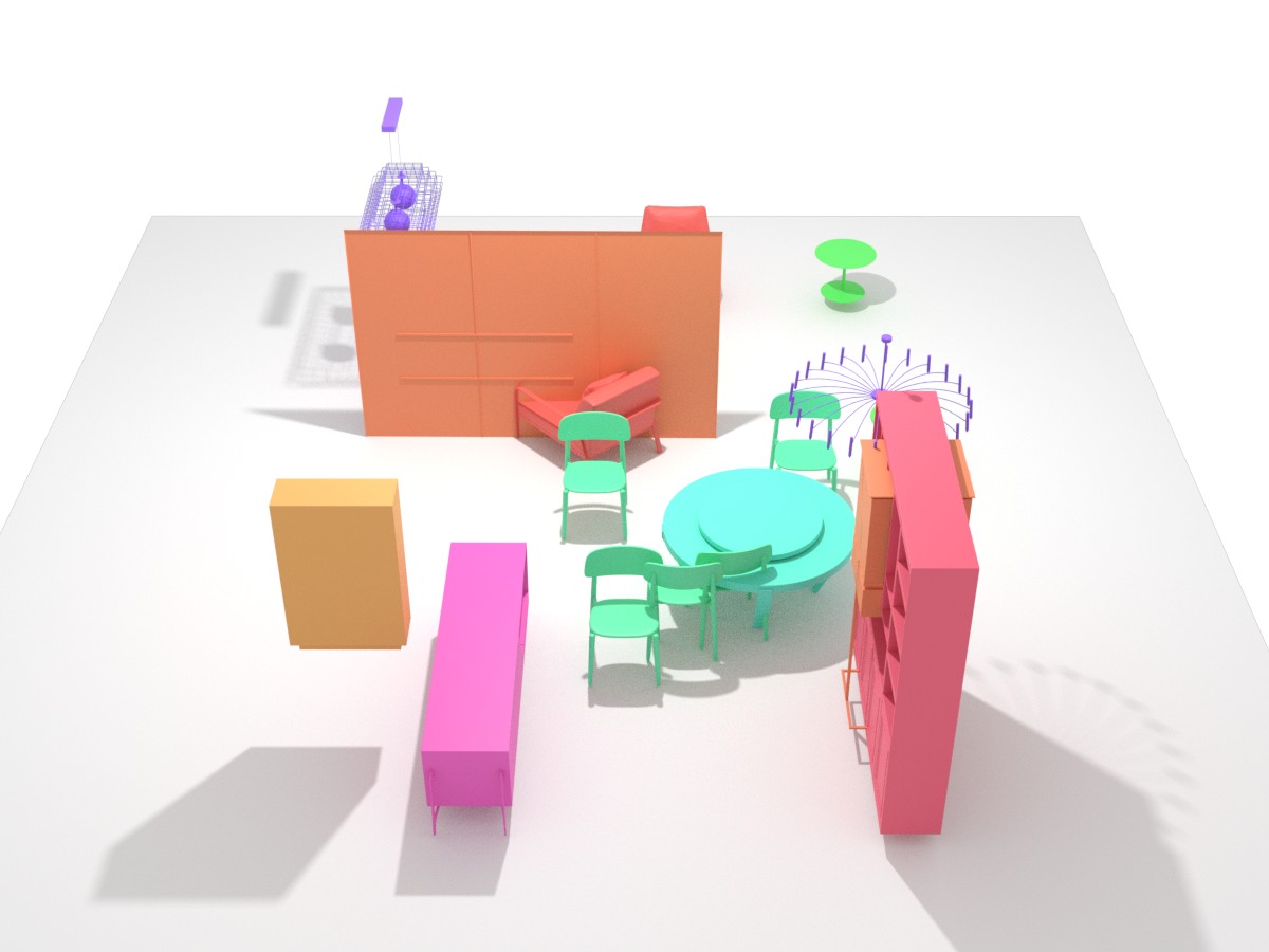
(b) ATISS [42]

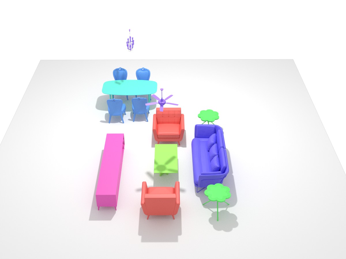
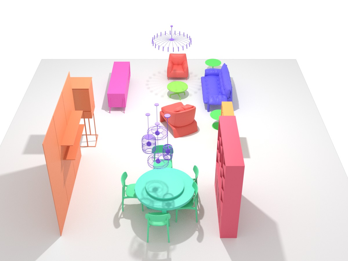
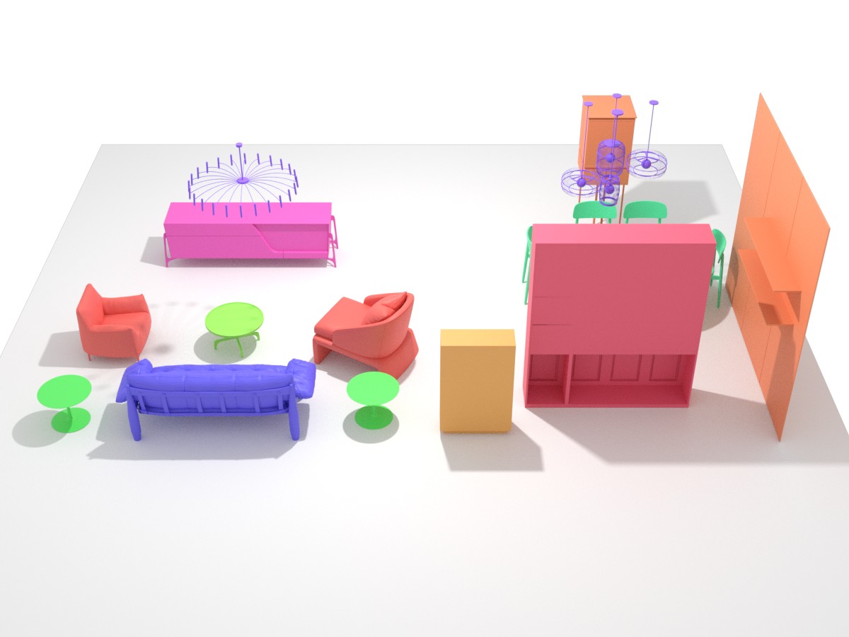
(c) Ours

Figure 11: Scene re-arrangements of collections of random objects. Compared to ATISS, our method generates various object placement options with better plausibility.

Method	Dining room			Living room
	FID $\downarrow$	KID $\downarrow$	SCA $\%$	FID $\downarrow$	KID $\downarrow$	SCA $\%$
ATISS	43.40	7.85	63.99	43.98	6.73	73.83
Ours	40.84	2.21	40.36	42.92	2.81	61.13

Table 4: Quantitative comparisons on the task of scene arrangement on the 3D-FRONT bedrooms and dining rooms. Given a collection of objects as inputs, we predict their locations and orientations to obtain object placements.

Method	Dining room			Living room
	FID $\downarrow$	KID $\downarrow$	SCA $\%$	FID $\downarrow$	KID $\downarrow$	SCA $\%$
ATISS	36.61	1.90	55.44	40.45	4.57	63.48
Ours	32.87	0.57	51.67	35.27	0.64	54.69

Table 5: Quantitative comparisons on the task of text-conditioned scene synthesis on the 3D-FRONT dining and living rooms.

We visualize additional qualitative comparisons on the task of scene arrangement in Fig. 11. Also, the quantitative results are shown in Tab. 4.

Text-conditioned Scene Synthesis

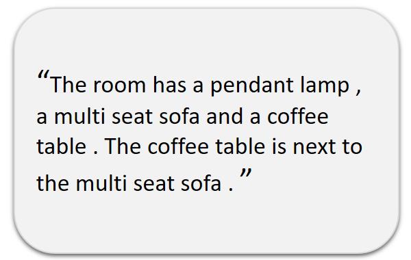
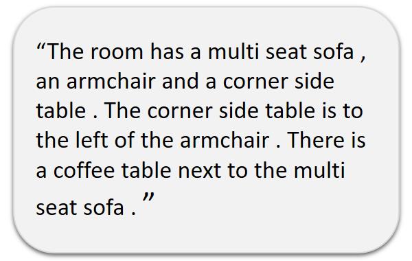
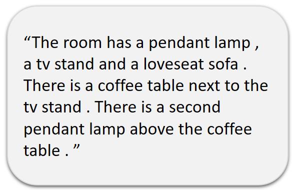
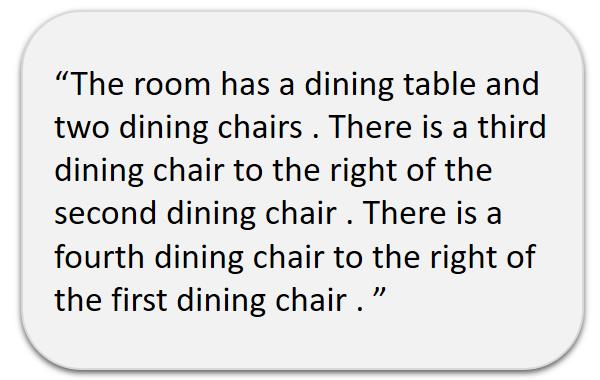
(a) Input text

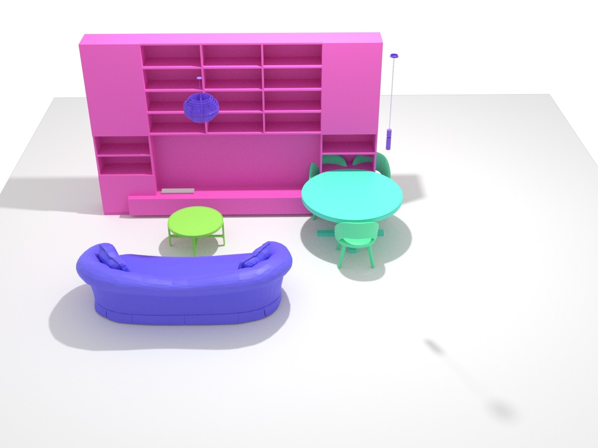
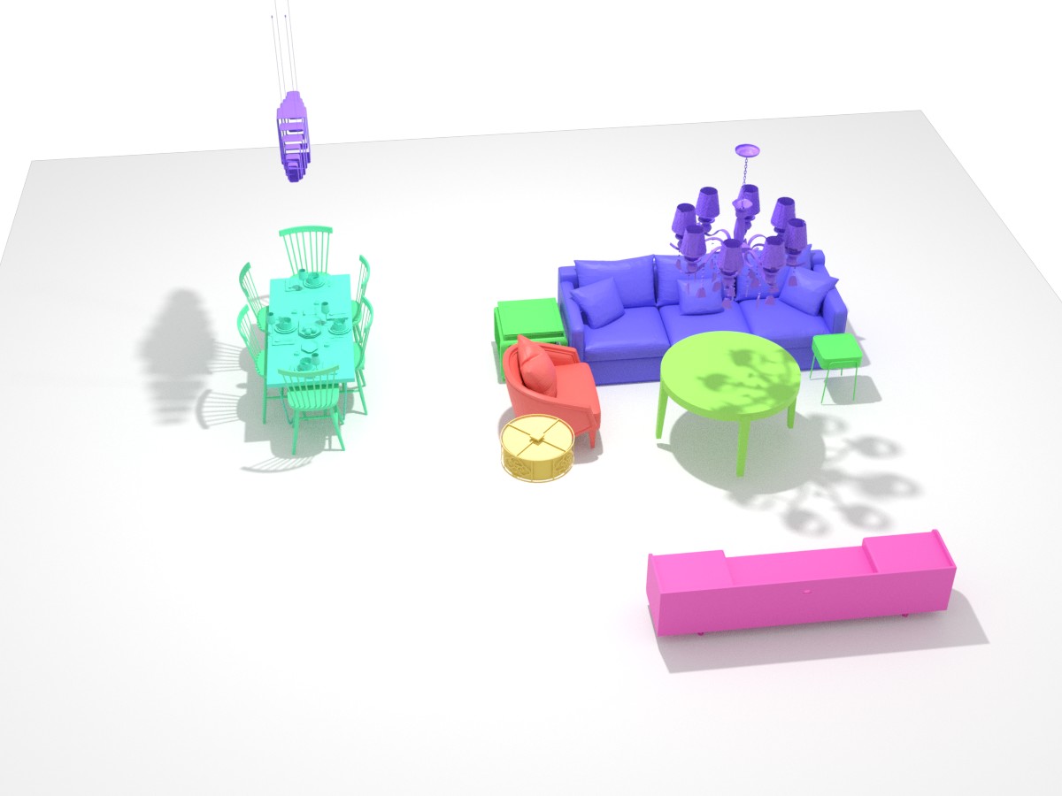
(b) Reference

(c) ATISS [42]

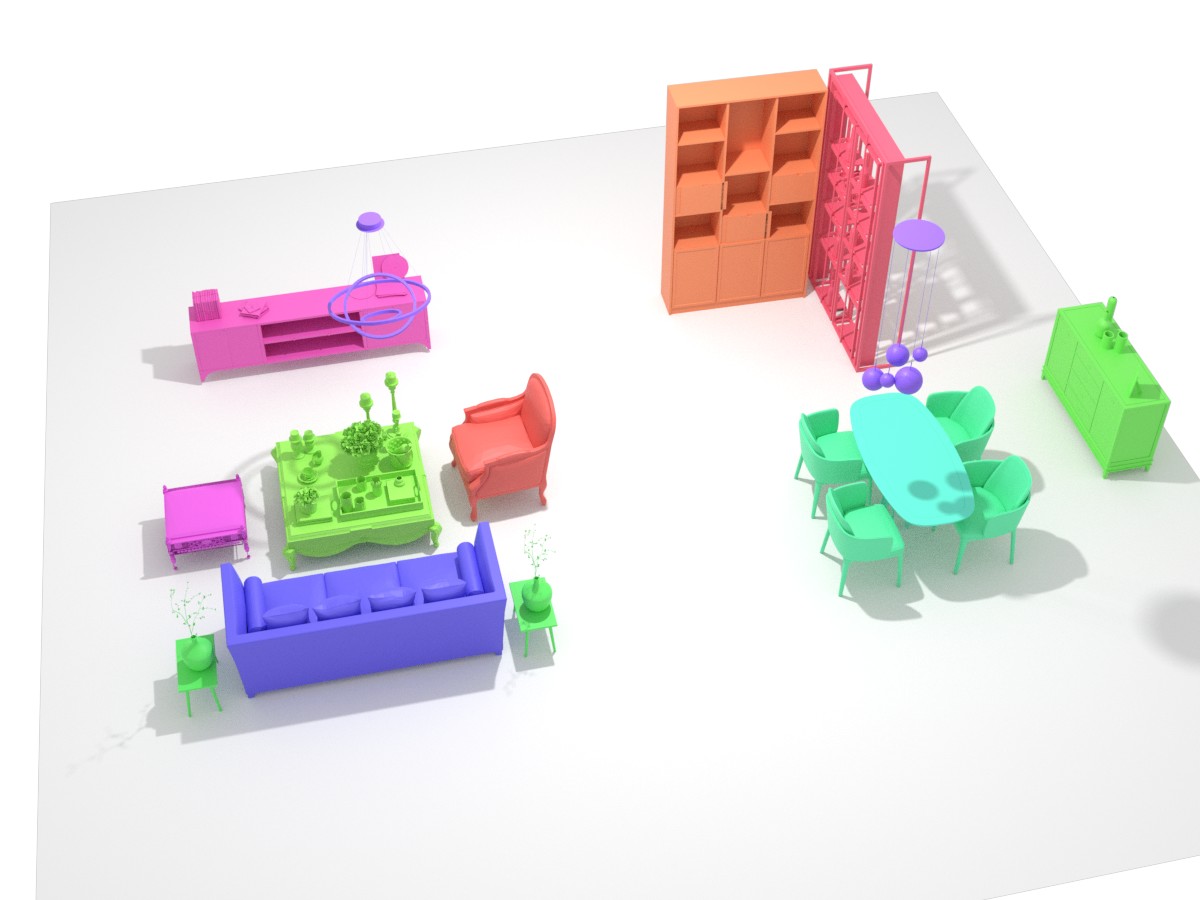
(d) Ours

Figure 12: Text-conditioned scene synthesis. The input text describes only a partial scene configuration. Our method generates more plausible scenes matched with the texts.

We provide additional qualitative comparisons on the text-conditioned scene synthesis in Fig. 12. As observed, in the first and third rows, ATISS has object intersection issues while ours does not. In the second row, our method can correctly generate a corner side table on the left of the armchair. However, ATISS generates a corner side table on the right of the armchair. In the fourth row, our method can generate four dining chairs that are consistent with the text description, but ATISS can only generate two dining chairs. The quantitative results evaluated by FID, KID, and SCA are reported in Tab. 5. Our method consistently outperforms ATISS in all used metrics.

Appendix E User Study

We conducted a perceptual user study to evaluate the quality of our method against ATISS on the application of text-conditioned scene synthesis. As shown in Fig. 13, we provide the visualization of a ground-truth scene used to generate a text prompt as a reference. For each pair of results, a user needs to answer “which of the generated scene can better match the text prompt?” and “Which of the generated scene is more reasonable and realistic?”. We collect the answers of 225 scenes from 45 users and calculate the statistics. 62$\%$ of the user answers prefer our method to ATISS in realism. 55$\%$ of answers think our method is more consistent with the text prompt.

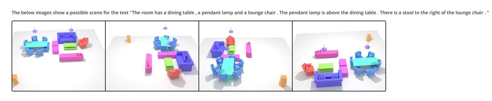
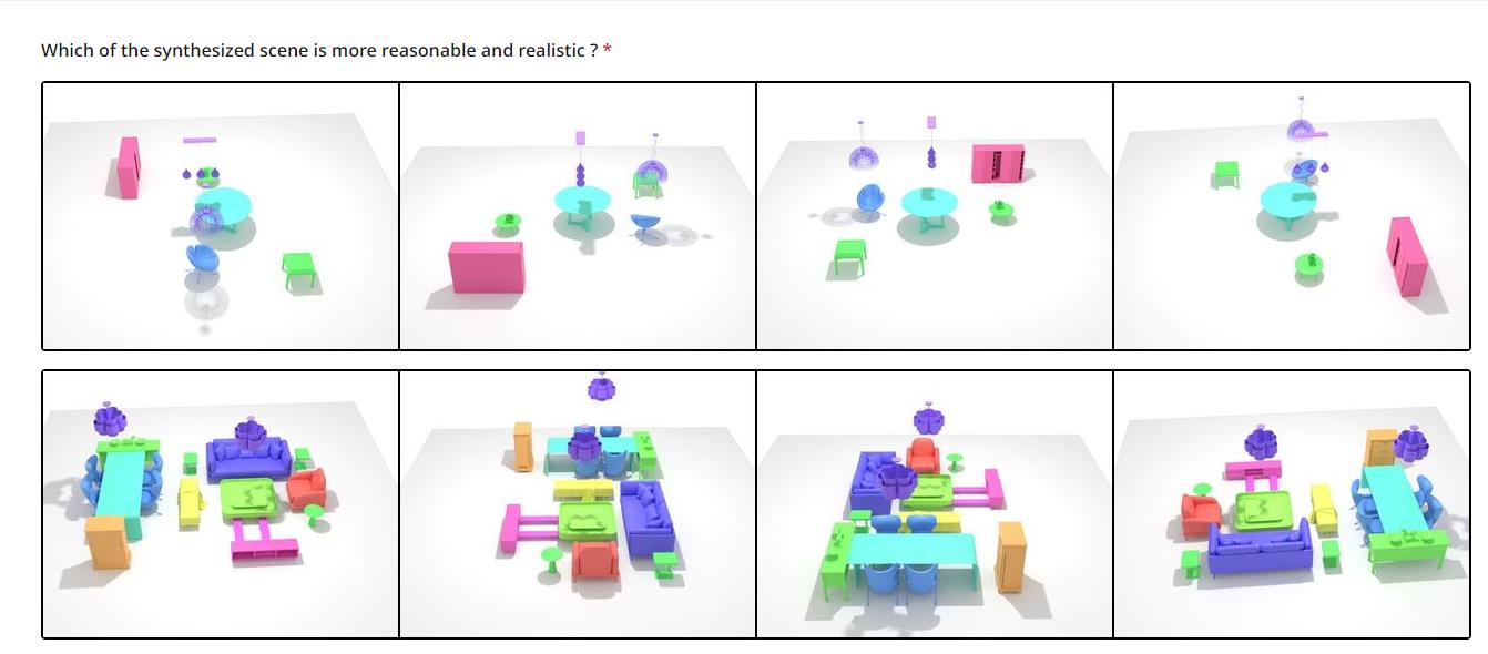
Figure 13: User Study UI. Based on the reference scene used to generate text prompts, users are asked which of the synthesized scene is more matched with the text prompt and more realistic. Note that the results from ATISS and our method are randomly shuffled to avoid bias.

References

- [1] Omri Avrahami, Dani Lischinski, and Ohad Fried. Blended diffusion for text-driven editing of natural images. In Proceedings of the IEEE/CVF Conference on Computer Vision and Pattern Recognition, pages 18208–18218, 2022.
- [2] Mikołaj Bińkowski, Danica J Sutherland, Michael Arbel, and Arthur Gretton. Demystifying mmd gans. arXiv preprint arXiv:1801.01401, 2018.
- [3] Angel Chang, Manolis Savva, and Christopher D Manning. Learning spatial knowledge for text to 3d scene generation. In Proceedings of the 2014 conference on empirical methods in natural language processing (EMNLP), pages 2028–2038, 2014.
- [4] Angel X Chang, Mihail Eric, Manolis Savva, and Christopher D Manning. Sceneseer: 3d scene design with natural language. arXiv preprint arXiv:1703.00050, 2017.
- [5] Ricky TQ Chen, Yulia Rubanova, Jesse Bettencourt, and David K Duvenaud. Neural ordinary differential equations. Advances in neural information processing systems, 31, 2018.
- [6] Zhiqin Chen and Hao Zhang. Learning implicit fields for generative shape modeling. In CVPR, 2019.
- [7] Christopher B Choy, Danfei Xu, JunYoung Gwak, Kevin Chen, and Silvio Savarese. 3d-r2n2: A unified approach for single and multi-view 3d object reconstruction. In Computer Vision–ECCV 2016: 14th European Conference, Amsterdam, The Netherlands, October 11-14, 2016, Proceedings, Part VIII 14, pages 628–644. Springer, 2016.
- [8] Angela Dai and Matthias Nießner. 3dmv: Joint 3d-multi-view prediction for 3d semantic scene segmentation. In Proceedings of the European Conference on Computer Vision (ECCV), pages 452–468, 2018.
- [9] Jacob Devlin, Ming-Wei Chang, Kenton Lee, and Kristina Toutanova. Bert: Pre-training of deep bidirectional transformers for language understanding. arXiv preprint arXiv:1810.04805, 2018.
- [10] Prafulla Dhariwal and Alexander Nichol. Diffusion models beat gans on image synthesis. Advances in Neural Information Processing Systems, 34:8780–8794, 2021.
- [11] Patrick Esser, Robin Rombach, and Bjorn Ommer. Taming transformers for high-resolution image synthesis. In Proceedings of the IEEE/CVF conference on computer vision and pattern recognition, pages 12873–12883, 2021.
- [12] Matthew Fisher and Pat Hanrahan. Context-based search for 3d models. In ACM SIGGRAPH Asia 2010 papers, pages 1–10. 2010.
- [13] Matthew Fisher, Daniel Ritchie, Manolis Savva, Thomas Funkhouser, and Pat Hanrahan. Example-based synthesis of 3d object arrangements. ACM Transactions on Graphics (TOG), 31(6):1–11, 2012.
- [14] Matthew Fisher, Manolis Savva, Yangyan Li, Pat Hanrahan, and Matthias Nießner. Activity-centric scene synthesis for functional 3d scene modeling. ACM Transactions on Graphics (TOG), 34(6):1–13, 2015.
- [15] Huan Fu, Bowen Cai, Lin Gao, Ling-Xiao Zhang, Jiaming Wang, Cao Li, Qixun Zeng, Chengyue Sun, Rongfei Jia, Binqiang Zhao, et al. 3d-front: 3d furnished rooms with layouts and semantics. In Proceedings of the IEEE/CVF International Conference on Computer Vision, pages 10933–10942, 2021.
- [16] Huan Fu, Rongfei Jia, Lin Gao, Mingming Gong, Binqiang Zhao, Steve Maybank, and Dacheng Tao. 3d-future: 3d furniture shape with texture. International Journal of Computer Vision, 129:3313–3337, 2021.
- [17] Qiang Fu, Xiaowu Chen, Xiaotian Wang, Sijia Wen, Bin Zhou, and Hongbo Fu. Adaptive synthesis of indoor scenes via activity-associated object relation graphs. ACM Transactions on Graphics (TOG), 36(6):1–13, 2017.
- [18] Ian Goodfellow, Jean Pouget-Abadie, Mehdi Mirza, Bing Xu, David Warde-Farley, Sherjil Ozair, Aaron Courville, and Yoshua Bengio. Generative adversarial networks. Communications of the ACM, 63(11):139–144, 2020.
- [19] Alex Graves. Generating sequences with recurrent neural networks. arXiv preprint arXiv:1308.0850, 2013.
- [20] Xiaoguang Han, Zhaoxuan Zhang, Dong Du, Mingdai Yang, Jingming Yu, Pan Pan, Xin Yang, Ligang Liu, Zixiang Xiong, and Shuguang Cui. Deep reinforcement learning of volume-guided progressive view inpainting for 3d point scene completion from a single depth image. In Proceedings of the IEEE/CVF Conference on Computer Vision and Pattern Recognition, pages 234–243, 2019.
- [21] Martin Heusel, Hubert Ramsauer, Thomas Unterthiner, Bernhard Nessler, and Sepp Hochreiter. Gans trained by a two time-scale update rule converge to a local nash equilibrium. Advances in neural information processing systems, 30, 2017.
- [22] Jonathan Ho, Ajay Jain, and Pieter Abbeel. Denoising diffusion probabilistic models. Advances in Neural Information Processing Systems, 33:6840–6851, 2020.
- [23] Jonathan Ho, Chitwan Saharia, William Chan, David J Fleet, Mohammad Norouzi, and Tim Salimans. Cascaded diffusion models for high fidelity image generation. J. Mach. Learn. Res., 23:47–1, 2022.
- [24] Jonathan Ho and Tim Salimans. Classifier-free diffusion guidance. arXiv preprint arXiv:2207.12598, 2022.
- [25] Jonathan Ho, Tim Salimans, Alexey Gritsenko, William Chan, Mohammad Norouzi, and David J Fleet. Video diffusion models. arXiv preprint arXiv:2204.03458, 2022.
- [26] Ka-Hei Hui, Ruihui Li, Jingyu Hu, and Chi-Wing Fu. Neural wavelet-domain diffusion for 3d shape generation. In SIGGRAPH Asia 2022 Conference Papers, pages 1–9, 2022.
- [27] Yun Jiang, Marcus Lim, and Ashutosh Saxena. Learning object arrangements in 3d scenes using human context. arXiv preprint arXiv:1206.6462, 2012.
- [28] Gwanghyun Kim, Taesung Kwon, and Jong Chul Ye. Diffusionclip: Text-guided diffusion models for robust image manipulation. In Proceedings of the IEEE/CVF Conference on Computer Vision and Pattern Recognition, pages 2426–2435, 2022.
- [29] Diederik P Kingma and Max Welling. Auto-encoding variational bayes. arXiv preprint arXiv:1312.6114, 2013.
- [30] Manyi Li, Akshay Gadi Patil, Kai Xu, Siddhartha Chaudhuri, Owais Khan, Ariel Shamir, Changhe Tu, Baoquan Chen, Daniel Cohen-Or, and Hao Zhang. Grains: Generative recursive autoencoders for indoor scenes. ACM Transactions on Graphics (TOG), 38(2):1–16, 2019.
- [31] Andreas Lugmayr, Martin Danelljan, Andres Romero, Fisher Yu, Radu Timofte, and Luc Van Gool. Repaint: Inpainting using denoising diffusion probabilistic models. In Proceedings of the IEEE/CVF Conference on Computer Vision and Pattern Recognition, pages 11461–11471, 2022.
- [32] Shitong Luo and Wei Hu. Diffusion probabilistic models for 3d point cloud generation. In Proceedings of the IEEE/CVF Conference on Computer Vision and Pattern Recognition, pages 2837–2845, 2021.
- [33] Rui Ma, Honghua Li, Changqing Zou, Zicheng Liao, Xin Tong, and Hao Zhang. Action-driven 3d indoor scene evolution. ACM Trans. Graph., 35(6):173–1, 2016.
- [34] Chenlin Meng, Yutong He, Yang Song, Jiaming Song, Jiajun Wu, Jun-Yan Zhu, and Stefano Ermon. Sdedit: Guided image synthesis and editing with stochastic differential equations. In International Conference on Learning Representations, 2021.
- [35] Paul Merrell, Eric Schkufza, Zeyang Li, Maneesh Agrawala, and Vladlen Koltun. Interactive furniture layout using interior design guidelines. ACM transactions on graphics (TOG), 30(4):1–10, 2011.
- [36] Lars Mescheder, Michael Oechsle, Michael Niemeyer, Sebastian Nowozin, and Andreas Geiger. Occupancy networks: Learning 3d reconstruction in function space. In CVPR, 2019.
- [37] Ben Mildenhall, Pratul P Srinivasan, Matthew Tancik, Jonathan T Barron, Ravi Ramamoorthi, and Ren Ng. Nerf: Representing scenes as neural radiance fields for view synthesis. Communications of the ACM, 65(1):99–106, 2021.
- [38] Alex Nichol, Prafulla Dhariwal, Aditya Ramesh, Pranav Shyam, Pamela Mishkin, Bob McGrew, Ilya Sutskever, and Mark Chen. Glide: Towards photorealistic image generation and editing with text-guided diffusion models. arXiv preprint arXiv:2112.10741, 2021.
- [39] Yinyu Nie, Angela Dai, Xiaoguang Han, and Matthias Nießner. Learning 3d scene priors with 2d supervision. arXiv preprint arXiv:2211.14157, 2022.
- [40] Yinyu Nie, Angela Dai, Xiaoguang Han, and Matthias Nießner. Pose2room: understanding 3d scenes from human activities. In Computer Vision–ECCV 2022: 17th European Conference, Tel Aviv, Israel, October 23–27, 2022, Proceedings, Part XXVII, pages 425–443. Springer, 2022.
- [41] Jeong Joon Park, Peter Florence, Julian Straub, Richard Newcombe, and Steven Lovegrove. Deepsdf: Learning continuous signed distance functions for shape representation. In CVPR, 2019.
- [42] Despoina Paschalidou, Amlan Kar, Maria Shugrina, Karsten Kreis, Andreas Geiger, and Sanja Fidler. Atiss: Autoregressive transformers for indoor scene synthesis. Advances in Neural Information Processing Systems, 34:12013–12026, 2021.
- [43] Ben Poole, Ajay Jain, Jonathan T Barron, and Ben Mildenhall. Dreamfusion: Text-to-3d using 2d diffusion. arXiv preprint arXiv:2209.14988, 2022.
- [44] Pulak Purkait, Christopher Zach, and Ian Reid. Sg-vae: Scene grammar variational autoencoder to generate new indoor scenes. In Computer Vision–ECCV 2020: 16th European Conference, Glasgow, UK, August 23–28, 2020, Proceedings, Part XXIV 16, pages 155–171. Springer, 2020.
- [45] Charles R Qi, Hao Su, Kaichun Mo, and Leonidas J Guibas. Pointnet: Deep learning on point sets for 3d classification and segmentation. In Proceedings of the IEEE conference on computer vision and pattern recognition, pages 652–660, 2017.
- [46] Siyuan Qi, Yixin Zhu, Siyuan Huang, Chenfanfu Jiang, and Song-Chun Zhu. Human-centric indoor scene synthesis using stochastic grammar. In Proceedings of the IEEE Conference on Computer Vision and Pattern Recognition, pages 5899–5908, 2018.
- [47] Aditya Ramesh, Prafulla Dhariwal, Alex Nichol, Casey Chu, and Mark Chen. Hierarchical text-conditional image generation with clip latents. arXiv preprint arXiv:2204.06125, 2022.
- [48] Ali Razavi, Aaron Van den Oord, and Oriol Vinyals. Generating diverse high-fidelity images with vq-vae-2. Advances in neural information processing systems, 32, 2019.
- [49] Danilo Rezende and Shakir Mohamed. Variational inference with normalizing flows. In International conference on machine learning, pages 1530–1538. PMLR, 2015.
- [50] Daniel Ritchie, Kai Wang, and Yu-an Lin. Fast and flexible indoor scene synthesis via deep convolutional generative models. In Proceedings of the IEEE/CVF Conference on Computer Vision and Pattern Recognition, pages 6182–6190, 2019.
- [51] Robin Rombach, Andreas Blattmann, Dominik Lorenz, Patrick Esser, and Björn Ommer. High-resolution image synthesis with latent diffusion models. In Proceedings of the IEEE/CVF Conference on Computer Vision and Pattern Recognition, pages 10684–10695, 2022.
- [52] Olaf Ronneberger, Philipp Fischer, and Thomas Brox. U-net: Convolutional networks for biomedical image segmentation. In Medical Image Computing and Computer-Assisted Intervention–MICCAI 2015: 18th International Conference, Munich, Germany, October 5-9, 2015, Proceedings, Part III 18, pages 234–241. Springer, 2015.
- [53] Chitwan Saharia, Jonathan Ho, William Chan, Tim Salimans, David J Fleet, and Mohammad Norouzi. Image super-resolution via iterative refinement. IEEE Transactions on Pattern Analysis and Machine Intelligence, 2022.
- [54] Manolis Savva, Angel X Chang, and Maneesh Agrawala. Scenesuggest: Context-driven 3d scene design. arXiv preprint arXiv:1703.00061, 2017.
- [55] Jascha Sohl-Dickstein, Eric Weiss, Niru Maheswaranathan, and Surya Ganguli. Deep unsupervised learning using nonequilibrium thermodynamics. In International Conference on Machine Learning, pages 2256–2265. PMLR, 2015.
- [56] Jiaming Song, Chenlin Meng, and Stefano Ermon. Denoising diffusion implicit models. arXiv preprint arXiv:2010.02502, 2020.
- [57] Yang Song and Stefano Ermon. Generative modeling by estimating gradients of the data distribution. Advances in Neural Information Processing Systems, 32, 2019.
- [58] Yang Song and Stefano Ermon. Improved techniques for training score-based generative models. Advances in neural information processing systems, 33:12438–12448, 2020.
- [59] Yang Song, Jascha Sohl-Dickstein, Diederik P Kingma, Abhishek Kumar, Stefano Ermon, and Ben Poole. Score-based generative modeling through stochastic differential equations. arXiv preprint arXiv:2011.13456, 2020.
- [60] Jiapeng Tang, Xiaoguang Han, Junyi Pan, Kui Jia, and Xin Tong. A skeleton-bridged deep learning approach for generating meshes of complex topologies from single rgb images. In Proceedings of the IEEE/CVF Conference on Computer Vision and Pattern Recognition, pages 4541–4550, 2019.
- [61] Jiapeng Tang, Jiabao Lei, Dan Xu, Feiying Ma, Kui Jia, and Lei Zhang. Sa-convonet: Sign-agnostic optimization of convolutional occupancy networks. In Proceedings of the IEEE/CVF International Conference on Computer Vision, pages 6504–6513, 2021.
- [62] Jiapeng Tang, Lev Markhasin, Bi Wang, Justus Thies, and Matthias Nießner. Neural shape deformation priors. In Advances in Neural Information Processing Systems, 2022.
- [63] Aaron Van den Oord, Nal Kalchbrenner, Lasse Espeholt, Oriol Vinyals, Alex Graves, et al. Conditional image generation with pixelcnn decoders. Advances in neural information processing systems, 29, 2016.
- [64] Aaron Van Den Oord, Oriol Vinyals, et al. Neural discrete representation learning. Advances in neural information processing systems, 30, 2017.
- [65] Ashish Vaswani, Noam Shazeer, Niki Parmar, Jakob Uszkoreit, Llion Jones, Aidan N Gomez, Łukasz Kaiser, and Illia Polosukhin. Attention is all you need. Advances in neural information processing systems, 30, 2017.
- [66] Kai Wang, Yu-An Lin, Ben Weissmann, Manolis Savva, Angel X Chang, and Daniel Ritchie. Planit: Planning and instantiating indoor scenes with relation graph and spatial prior networks. ACM Transactions on Graphics (TOG), 38(4):1–15, 2019.
- [67] Kai Wang, Manolis Savva, Angel X Chang, and Daniel Ritchie. Deep convolutional priors for indoor scene synthesis. ACM Transactions on Graphics (TOG), 37(4):1–14, 2018.
- [68] Xinpeng Wang, Chandan Yeshwanth, and Matthias Nießner. Sceneformer: Indoor scene generation with transformers. In 2021 International Conference on 3D Vision (3DV), pages 106–115. IEEE, 2021.
- [69] Yue Wang, Yongbin Sun, Ziwei Liu, Sanjay E Sarma, Michael M Bronstein, and Justin M Solomon. Dynamic graph cnn for learning on point clouds. Acm Transactions On Graphics (tog), 38(5):1–12, 2019.
- [70] Jiajun Wu, Chengkai Zhang, Tianfan Xue, Bill Freeman, and Josh Tenenbaum. Learning a probabilistic latent space of object shapes via 3d generative-adversarial modeling. Advances in neural information processing systems, 29, 2016.
- [71] Zhisheng Xiao, Karsten Kreis, and Arash Vahdat. Tackling the generative learning trilemma with denoising diffusion gans. arXiv preprint arXiv:2112.07804, 2021.
- [72] Kun Xu, Kang Chen, Hongbo Fu, Wei-Lun Sun, and Shi-Min Hu. Sketch2scene: Sketch-based co-retrieval and co-placement of 3d models. ACM Transactions on Graphics (TOG), 32(4):1–15, 2013.
- [73] Haitao Yang, Zaiwei Zhang, Siming Yan, Haibin Huang, Chongyang Ma, Yi Zheng, Chandrajit Bajaj, and Qixing Huang. Scene synthesis via uncertainty-driven attribute synchronization. In Proceedings of the IEEE/CVF International Conference on Computer Vision, pages 5630–5640, 2021.
- [74] Ming-Jia Yang, Yu-Xiao Guo, Bin Zhou, and Xin Tong. Indoor scene generation from a collection of semantic-segmented depth images. In Proceedings of the IEEE/CVF International Conference on Computer Vision, pages 15203–15212, 2021.
- [75] Ruihan Yang, Prakhar Srivastava, and Stephan Mandt. Diffusion probabilistic modeling for video generation. arXiv preprint arXiv:2203.09481, 2022.
- [76] Yaoqing Yang, Chen Feng, Yiru Shen, and Dong Tian. Foldingnet: Point cloud auto-encoder via deep grid deformation. In Proceedings of the IEEE conference on computer vision and pattern recognition, pages 206–215, 2018.
- [77] Yi-Ting Yeh, Lingfeng Yang, Matthew Watson, Noah D Goodman, and Pat Hanrahan. Synthesizing open worlds with constraints using locally annealed reversible jump mcmc. ACM Transactions on Graphics (TOG), 31(4):1–11, 2012.
- [78] Tianwei Yin, Xingyi Zhou, and Philipp Krahenbuhl. Center-based 3d object detection and tracking. In Proceedings of the IEEE/CVF conference on computer vision and pattern recognition, pages 11784–11793, 2021.
- [79] Lap Fai Yu, Sai Kit Yeung, Chi Keung Tang, Demetri Terzopoulos, Tony F Chan, and Stanley J Osher. Make it home: automatic optimization of furniture arrangement. ACM Transactions on Graphics (TOG)-Proceedings of ACM SIGGRAPH 2011, v. 30,(4), July 2011, article no. 86, 30(4), 2011.
- [80] Sihao Yu, Fei Sun, Jiafeng Guo, Ruqing Zhang, and Xueqi Cheng. Legonet: A fast and exact unlearning architecture. arXiv preprint arXiv:2210.16023, 2022.
- [81] Xiaohui Zeng, Arash Vahdat, Francis Williams, Zan Gojcic, Or Litany, Sanja Fidler, and Karsten Kreis. Lion: Latent point diffusion models for 3d shape generation. arXiv preprint arXiv:2210.06978, 2022.
- [82] Biao Zhang, Jiapeng Tang, Matthias Niessner, and Peter Wonka. 3dshape2vecset: A 3d shape representation for neural fields and generative diffusion models. arXiv preprint arXiv:2301.11445, 2023.
- [83] Zaiwei Zhang, Zhenpei Yang, Chongyang Ma, Linjie Luo, Alexander Huth, Etienne Vouga, and Qixing Huang. Deep generative modeling for scene synthesis via hybrid representations. ACM Transactions on Graphics (TOG), 39(2):1–21, 2020.
- [84] Linqi Zhou, Yilun Du, and Jiajun Wu. 3d shape generation and completion through point-voxel diffusion. In Proceedings of the IEEE/CVF International Conference on Computer Vision, pages 5826–5835, 2021.
- [85] Ji-Zhao Zhu, Yan-Tao Jia, Jun Xu, Jian-Zhong Qiao, and Xue-Qi Cheng. Modeling the correlations of relations for knowledge graph embedding. Journal of Computer Science and Technology, 33:323–334, 2018.