Abstract

The BFSS matrix model relates flat space M-theory to a large $N$ limit of matrix quantum mechanics describing $N$ non-relativistic D0-branes. M-theory, being a theory of gravity in flat space, has a rich infrared structure that includes various soft theorems and an infinite set of conserved charges associated to asymptotic symmetries. In this work, we ask: to what extent is this infrared structure present in BFSS? We find that all the salient features concerning the infrared structure of M-theory carry over naturally to the quantum mechanics dual. Moreover, we demonstrate that the dual statement of the soft graviton theorem in the matrix model implies that D0-brane scattering amplitudes in BFSS enjoy the full $11$d Lorentz symmetry of M-theory, a claim which has been long anticipated. We also offer several first-principle consistency checks for our findings, including a computation of the soft theorem which does not presuppose the BFSS duality and a non-trivial match between several known symmetries of M-theory and BFSS that appear naturally in this formalism. These calculations give non-perturbative evidence in support of the BFSS duality as a model of flat space holography.

1 Introduction

Although the holographic principle has a well-understood manifestation in asymptotically anti-de Sitter (AdS) spacetimes by way of the AdS/CFT correspondence [1], it has proved challenging to extend this paradigm to asymptotically flat spacetimes. Nevertheless, a holographic description of quantum gravity in asymptotically flat spacetimes seems plausible due to some underlying similarities with AdS. Indeed, the gravitational Hamiltonian is still a boundary term and the entropy of a black hole still scales like its area [2].

Historically, there have been two seemingly different approaches to flat space holography. The first is a top-down construction provided by the Banks-Fischler-Shenker-Susskind (BFSS) matrix model, which relates M-theory in flat spacetime to a theory of matrix quantum mechanics describing non-relativistic D0-branes in type IIA string theory [3, 4, 5, 6, 7, 8, 9, 10, 11]. This approach endeavors to provide a full non-perturbative duality for M-theory in flat space, and several non-trivial consistency checks have been performed [12, 13, 14, 15, 10, 11, 16, 17]. On the other hand, there have only been a few tests of this duality, and most of them concern a very specific setup: $2\rightarrow 2$ elastic scattering in the eikonal limit. Moreover, recovering the symmetries of M-theory in the dual description has remained a challenging open problem. Even the simplest question of demonstrating that BFSS enjoys 11d Lorentz symmetry has previously been elusive.

The other approach to flat space holography is celestial conformal field theory which aims to use null infinity ($\mathcal{I}^{\pm}$) as the celestial hologram [18, 19, 20, 21, 22, 23]. The kinematics of this approach to flat space holography are extremely well understood, in stark contrast with efforts to analyze BFSS. The Lorentz group manifests itself as the conformal group in the boundary theory, and certain so-called asymptotic symmetries, which generalize the Poincaré group, play a natural role in the boundary description. Understanding the dynamics of the duality is much more challenging, however. For the most part, this approach to flat space holography is explicitly bottom-up, translating scattering amplitudes in a bulk quantum theory to conformally-covariant correlation functions of operators which live on $\mathcal{I}^{\pm}$.

The overarching goal of this work is to use concepts recently developed in the context of celestial CFT to re-analyze certain properties of the BFSS matrix model. In particular, we will discuss the infrared structure of M-theory and see how these features are manifested in the matrix theory dual. This approach offers precise predictions about D0-brane quantum mechanics; in so doing, it gives an additional route to test the BFSS duality which has been previously unexplored in the literature. Notably, it gives a universal relation for D0-brane scattering amplitudes and allows one to see how the whole asymptotic symmetry group of M-theory (including, in particular, the full 11d Lorentz symmetry) is manifested in the dual description. Much of the work is focused on translating concrete statements about the infrared structure of M-theory to the D0-brane description by way of the BFSS duality; however, we also offer several first-principle consistency checks of these conjectures. As such, this manuscript gives a new, non-perturbative set of evidence for the BFSS duality as a holographic model of flat space M-theory.

The organization of the article is as follows. In Section 2, we will review the BFSS duality and survey how supergraviton scattering amplitudes in M-theory are realized in the matrix quantum mechanics. In Section 3, we will discuss the infrared structure of M-theory with a focus on soft theorems, conserved charges, and their corresponding asymptotic symmetries. In Sections 4, 5, and 6, we will analyze the dual description for these three concepts in the matrix model with an emphasis on demonstrating that BFSS scattering amplitudes enjoy a full 11d Lorentz symmetry as implied by the existence of soft theorems. The fact that the subleading soft graviton theorem implies Lorentz symmetry in generic theories of gravity has only been recently appreciated and is the main conceptual insight that we leverage to argue that $11$d Lorentz symmetry is also enjoyed by the $0+1$ dimensional matrix model [30, 31].

This work is a continuation of [32], which gave the original statement of the soft theorem in the matrix model and its relation to asymptotic symmetries of the RR 1-form gauge field in type IIA string theory.

2 Review of the BFSS Duality

The BFSS duality suggests that the full non-perturbative description of M-theory in 11d Minkowski spacetime is captured by a certain non-relativistic limit of D0-branes in type IIA string theory [17, 3, 4, 16, 5, 6, 7, 8, 9]. In this section, we review some salient aspects of this duality; familiar readers may safely skip it.

2.1 The BFSS Matrix Model

We begin by considering M-theory in flat 11d spacetime in lightcone coordinates $(x^{+},x^{-},x^{I})$ where $x^{\pm}=\tfrac{1}{\sqrt{2}}(x^{0}\pm x^{10})$ are the so-called longitudinal coordinates and $x^{I}$ are the transverse coordinates with $I\in\{1,...,9\}.$ In this setup, the longitudinal coordinate $x^{+}$ plays the role of time, and the momentum operator $P^{-}$ which translates between surfaces of constant $x^{+}$ is the Hamiltonian.

The BFSS Hamiltonian

The BFSS duality concerns the discrete lightcone quantization (DLCQ) of M-theory where the other longitudinal coordinate is compactified and the conjugate momentum is, therefore, quantized

$$x^{-}\sim x^{-}+2\pi R\hskip 30.0ptp^{+}=N/R.$$ (2.1)

Here, $N\in\mathbb{N}$ is a positive integer parametrizing the total momentum of a particular M-theory setup. The BFSS duality states that the sector of DLCQ M-theory with total momentum $p^{+}=N/R$ is dual to a model of matrix quantum mechanics where the fundamental degrees of freedom are $N\times N$ Hermitian matrices. The dynamics of these matrices are governed by the Hamiltonian

$$H_{\text{BFSS}}=\frac{R}{2}\hskip 2.0pt\text{Tr}\Bigg{[}P^{I}P^{I}-\frac{1}{2}[X^{I},X^{J}][X^{I},X^{J}]-\Psi^{T}\Gamma^{I}[X^{I},\Psi]\bigg{]},$$ (2.2)

where $X^{I}$ is a 9-component vector of $SO(9)$ with $P^{I}$ its conjugate momentum, $\Psi^{\alpha}$ is a 16-component spinor of $\text{Spin}(9)$, and $\Gamma^{I}_{\alpha\beta}$ are the gamma matrices of $\text{Spin}(9)$. All the fields are valued in the adjoint representation of $\mathfrak{u}(N)$. The physical Hilbert space of the theory is subject to the Gauss-law constraint which forces physical states to transform as $U(N)$ singlets.

BFSS as a Theory of Non-Relativistic D0-Branes

The BFSS Hamiltonian has a remarkable relationship with D0-brane quantum mechanics [33, 34, 35, 36, 37, 38]. The matrices $X^{I}$ encode the positions of $N$ D0-branes – an interpretation that becomes especially clear in the classical limit. Classically, the bosonic potential $V\sim-\text{Tr}([X^{I},X^{J}][X^{I},X^{J}])$ is minimized when the $X^{I}$ matrices are mutually commuting. Therefore, they may be simultaneously diagonalized with eigenvalues tracking the positions of the D0-branes. For example, $N$ non-interacting D0-branes with trajectories $x_{1}^{I}(t),...,x_{N}^{I}(t)$ are classically described by the diagonal matrices

$$X^{I}_{\text{cl.}}(t)=\begin{pmatrix}x^{I}_{1}(t)&&\\ &\ddots&\\ &&x^{I}_{N}(t)\end{pmatrix}.$$ (2.3)

Quantum mechanically, the problem becomes much more subtle; the state is no longer described by an individual matrix, $X^{I}_{\text{cl.}}$, but rather by a wavefunction over matrices $\Psi[X^{I}]$. This wavefunction is now supported on matrices of the form

$$X^{I}(t)=X^{I}_{\text{cl.}}(t)+\sqrt{\hbar}\hskip 1.0pt\Delta X^{I}(t),$$ (2.4)

where the $(i,j)$ component of the matrix of quantum fluctuations $\Delta X^{I}(t)$ is due to interactions between the $i^{th}$ and $j^{th}$ D0-branes via open strings stretched between the two. We have explicitly inserted a factor of $\sqrt{\hbar}$ into the above to emphasize that the fluctuations are quantum corrections.

2.2 Asymptotic States and Scattering Amplitudes

Now that both sides of the duality have been stated explicitly, it is important to understand precisely what observables agree between DLCQ M-theory and D0-brane quantum mechanics. Principally, we will be concerned with how S-matrix elements in M-theory are reproduced by corresponding S-matrix elements in BFSS.

In this work, we will only study scattering amplitudes among the supergraviton multiplet in M-theory and the corresponding states in the BFSS matrix model. This is because the infrared structure of M-theory is determined entirely by its massless modes, whose spectrum is captured by 11-dimensional $\mathcal{N}=1$ supergravity.

Supergraviton Scattering in M-theory

Supergravitons in M-theory are labelled by their energy-momentum vector, $p^{\mu},$ and polarization, $\Theta.$ It is convenient to parametrize the energy-momentum vectors in Cartesian coordinates by an overall scale $\omega\in\mathbb{R}_{\geq 0}$ and a nine-dimensional vector $v^{I}\in\mathbb{R}^{9}$ according to

$$p^{\mu}=\frac{\omega}{\sqrt{2}}(1+v^{\hskip 1.0pt2},2v^{I},1-v^{\hskip 1.0pt2}),$$ (2.5)

which satisfies the mass shell condition $p^{2}=0$ for arbitrary $(\omega,v^{I}).$ The polarization $\Theta$ labels how the state transforms under its little group. The supergraviton multiplet includes a graviton, a three-form gauge field, and a gravitino, which together transform in the $\textbf{44}\oplus\textbf{84}\oplus\textbf{128}$ representation of $SO(9).$

Defining S-matrix elements among supergraviton states in M-theory proceeds in the usual way. One considers the overlap of an in-state composed of $m$ widely separated supergravitons $|p^{\mu}_{1},\Theta_{1},...,p^{\mu}_{m},\Theta_{m}\rangle_{\text{in}}$ and a similarly constructed out state $|p_{m+1}^{\mu},\Theta_{m+1},...,p_{n}^{\mu},\Theta_{n}\rangle_{\text{out}}$

$$\mathcal{A}_{\text{M}}(p_{1}^{\mu},\Theta_{1},...,p_{n}^{\mu},\Theta_{n})=~{}_{\text{out}}\langle p_{m+1}^{\mu},\Theta_{m+1},...,p_{n}^{\mu},\Theta_{n}|p_{1}^{\mu},\Theta_{1},...,p_{m}^{\mu},\Theta_{m}\rangle_{\text{in}}.$$ (2.6)

D0-Brane Scattering in BFSS

One can also define scattering amplitudes among D0-branes and their bound states in an analogous manner [39, 40, 41, 42, 12, 13]. Each D0-brane bound state is labelled completely by the quantum numbers $N_{j}$ (the number of D0-branes in the bound state), $v_{j}^{I}$ (the velocity of the D0-brane bound state in the nine spatial directions), and $\Theta_{j}$ (a $2^{8}$-dimensional polarization vector transforming in the $\textbf{44}\oplus\textbf{84}\oplus\textbf{128}$ representation of $SO(9)$).

States with multiple, widely separated D0-brane bound states can also be constructed and are labelled respectively by the quantum numbers of the constituent particles. In this way, one can define incoming states $|N_{1},v_{1}^{I},\Theta_{1},...,N_{m},v_{m}^{I},\Theta_{m}\rangle_{\text{in}}$ and the corresponding outgoing states $|N_{m+1},v_{m+1},\Theta_{m+1},...,N_{n},v_{n},\Theta_{n}\rangle_{\text{out}}$ with $N=N_{1}+\cdots+N_{m}=N_{m+1}+\cdots+N_{n}$. The outgoing states are related to the incoming ones via time evolution with the BFSS Hamiltonian. Scattering amplitudes in the BFSS matrix model are defined by considering the overlap of such states

$$\begin{split}\mathcal{A}_{\text{BFSS}}(N_{1},v_{1}^{I},&\Theta_{1},...,N_{n},v_{n}^{I},\Theta_{n})\\ &=~{}_{\text{out}}\langle N_{m+1},v_{m+1}^{I},\Theta_{m+1},...,N_{n},v_{n}^{I},\Theta_{n}|N_{1},v_{1}^{I},\Theta_{1},...,N_{m},v_{m}^{I},\Theta_{m}\rangle_{\text{in}}.\end{split}$$ (2.7)

The BFSS Duality Dictionary

It is no coincidence that the quantum numbers describing supergravitons and those describing D0-brane bound states are so similar. Indeed, it is well-known that supergraviton states in DLCQ M-theory are dual to bound states of D0-branes in the matrix model [3, 4, 16, 43]. The parameters are related via Table 1. Moreover, the duality asserts that supergraviton scattering amplitudes agree with D0-brane scattering amplitudes when the parameters are related by this duality dictionary

$$\mathcal{A}_{\text{M}}(p_{1}^{\mu},\Theta_{1},...,p_{n}^{\mu},\Theta_{n})=\mathcal{A}_{\text{BFSS}}(N_{1},v_{1}^{I},\Theta_{1},...,N_{n},v_{n}^{I},\Theta_{n}).$$ (2.8)

M-Theory                             BFSS
$p_{j}^{+}$              $\Longleftrightarrow$               ${\frac{N_{j}}{R}}$
$p_{j}^{I}$               $\Longleftrightarrow$          $\sqrt{2}{\frac{N_{j}}{R}}v_{j}^{I}$
$p_{j}^{-}$              $\Longleftrightarrow$             ${\frac{N_{j}}{R}}v_{j}^{2}$
$\Theta_{j}$               $\Longleftrightarrow$               $\Theta_{j}$

Table 1: Dictionary between the kinematic data of gravitons in M-theory and D0-brane clumps in the matrix model. The relation concerning $p_{j}^{-}$ is determined using the mass-shell condition for M-theory gravitons $0=-2p_{j}^{+}p_{j}^{-}+p_{j}^{I}p_{j}^{I}$.

There have been several previous checks that scattering amplitudes in the two theories agree (e.g. [12, 13, 14, 15, 10, 11]); however, explicit calculations have only been performed in the low-energy, elastic limit of supergraviton scattering in M-theory, and many puzzles remain [44, 45, 46, 7].

In this article, we assume that BFSS provides an exact duality between scattering amplitudes in M-theory and those in D0-brane quantum mechanics. Specifically, even though a full understanding of BFSS is lacking, we will use Equation (2.8) to infer conjectures about the IR structure of the BFSS matrix model. Fortunately, we also provide significant first-principle evidence for this IR structure which is agnostic to the BFSS duality and does not presuppose Equation (2.8). This, in turn, supplies additional consistency checks of Equation (2.8) and supports the veracity of the BFSS duality as a whole.

The Decompactified M-Theory Limit

Up to this point, we have been equating amplitudes in the discrete lightcone quantization of M-theory with amplitudes in the BFSS matrix model at finite $N$. To recover scattering amplitudes in uncompactified M-theory, one sends the radius of compactification to infinity while holding the external momentum fixed [3, 4]

$$R\rightarrow\infty\hskip 30.0ptp_{j}^{\mu}=\text{const.}$$ (2.9)

Using the duality dictionary, we find that this is equivalent to the following scaling limit of the matrix model where the number of D0-branes in a particular bound state becomes infinitely large

$$R\sim N\sim N_{j}\rightarrow\infty\hskip 30.0ptv_{j}^{I}=\text{const.}\hskip 52.0pt$$ (2.10)

3 Infrared Structure of M-theory

It is well-known that all gravitational theories in asymptotically flat spacetime exhibit certain universal features. As M-theory includes gravitons, these universal results are applicable and provide interesting non-perturbative information about the infrared structure of M-theory. In this section, we discuss how supergraviton scattering amplitudes obey precise soft theorems. We also review how these soft theorems are equivalent to Ward identities enforcing the conservation of infinitely many charges associated to asymptotic symmetries.

3.1 Soft Theorems

Consider a generic $(n+1)$-particle scattering amplitude which includes a graviton with momentum $q_{s}^{\mu}$ and polarization tensor $\varepsilon^{\mu\nu}$ among its external states. We write this amplitude as $\mathcal{A}_{\text{M}}(q_{s}^{\mu},\varepsilon;p_{1}^{\mu},...,p_{n}^{\mu})$ where $p_{1}^{\mu},...,p^{\mu}_{n}$ label the future-directed momenta of the other $n$ particles. We will focus on the case where the other particles are also supergraviton states, though the result holds even outside of this setting.

The soft graviton theorem demonstrates that this amplitude obeys a universal factorization property in the limit $\omega_{s}/\omega_{j}\rightarrow 0$ where $\omega_{s}$ (respectively $\omega_{j}$) is the overall scale of $q_{s}^{\mu}$ (respectively $p_{j}^{\mu}$) as defined in Equation (2.5) [1, 47, 48, 49, 27, 50, 51]. This is the so-called soft limit, and one may perform a series expansion of the amplitude in this ratio. The soft graviton theorem states

$$\mathcal{A}_{\text{M}}(q_{s}^{\mu},\varepsilon;p_{1}^{\mu},...,p_{n}^{\mu})=\Big{[}\mathcal{S}^{(-1)}+\mathcal{S}^{(0)}+\cdots\Big{]}\mathcal{A}_{\text{M}}(p_{1}^{\mu},...,p_{n}^{\mu})\hskip 30.0pt\text{where}\hskip 30.0pt\mathcal{S}^{(n)}~{}\propto~{}\Big{(}\frac{\omega_{s}}{\omega_{j}}\Big{)}^{n}$$ (3.1)

and so relates an amplitude with a soft graviton to an amplitude without one. Moreover, it has been demonstrated that $\mathcal{S}^{(-1)}$ and $\mathcal{S}^{(0)}$ take the following universal form [1, 51]

$$\mathcal{S}^{(-1)}=\frac{\kappa}{2}\hskip 2.0pt\varepsilon_{\mu\nu}\sum_{j=1}^{n}\eta_{s}\eta_{j}\frac{p_{j}^{\mu}p_{j}^{\nu}}{q_{s}\cdot p_{j}}\hskip 35.0pt\mathcal{S}^{(0)}=i\frac{\kappa}{2}\varepsilon_{\mu\nu}\sum_{j=1}^{n}\eta_{s}\eta_{j}\frac{p^{\mu}_{j}J^{\nu\rho}_{j}q_{s,\rho}}{q_{s}\cdot p_{j}},$$ (3.2)

where $\kappa=\sqrt{32\pi G_{N}}$ is Newtons’s constant, and we have defined $\eta_{j}=-1$ if particle $j$ is incoming and $\eta_{j}=+1$ if the particle $j$ is outgoing (similarly for $\eta_{s}$). $\mathcal{S}^{(-1)}$ is called the leading soft term while $\mathcal{S}^{(0)}$ is called the sub-leading soft term. Note that the leading soft term has a pole $\propto~{}(\omega_{s}/\omega_{j})^{-1}$, so the amplitude diverges in the soft limit. Finally, $J^{\mu\nu}_{j}$ is the generator of angular momentum of the $j^{th}$ particle and is composed of both orbital and spin operators

$$J^{\mu\nu}_{j}=L^{\mu\nu}_{j}+S^{\mu\nu}_{j}.$$ (3.3)

In general, there will also be sub-subleading terms in the soft expansion which have positive powers of $(\omega_{s}/\omega_{j})$ in the soft limit; however, these terms are theory dependent and won’t play a role in our analysis.

3.2 Conservation Laws

The leading and subleading soft graviton theorems have been shown to be equivalent to Ward identities which enforce various symmetries in scattering amplitudes. To this end, it is convenient to express the $n$-particle amplitude as the overlap of incoming and outgoing multi-supergraviton states according to Equation (2.6). To simplify the notation, we will use the shorthand $|\text{in}\rangle=|p_{1}^{\mu},\Theta_{1},...,p_{m}^{\mu},\Theta_{m}\rangle_{\text{in}}$ and $|\text{out}\rangle=|p_{m+1}^{\mu},\Theta_{m+1},...,p_{n}^{\mu},\Theta_{n}\rangle_{\text{out}}$ to stand in for these states.

Next, we define the creation operator $G_{IJ}^{\hskip 1.0pt\text{in}\dagger}(\omega_{s},v_{s})$ for an incoming graviton state with momentum $q_{s}^{\mu}$ parameterized by $(\omega_{s},v_{s})$ and polarization tensor $\varepsilon^{\mu\nu}=(\varepsilon_{IJ})^{\mu\nu}$. Here, $(\varepsilon_{IJ})^{\mu\nu}$ are defined by

$$(\varepsilon_{IJ})^{\mu\nu}=\frac{1}{2}(\varepsilon^{\mu}_{I}\varepsilon^{\nu}_{J}+\varepsilon^{\nu}_{I}\varepsilon^{\mu}_{J})-\frac{1}{9}\delta_{IJ}\varepsilon^{\mu}_{K}\varepsilon^{K\nu}\hskip 30.0pt\text{with}\hskip 30.0pt\varepsilon^{\mu}_{J}=(v^{J}_{s},\delta^{I}_{J},-v^{J}_{s}).$$ (3.4)

They are symmetric and traceless in the $I,J=1,...,9$ indices and form a basis for the graviton’s 44 polarization states. One may similarly define the operator $G_{IJ}^{\hskip 1.0pt\text{out}\dagger}(\omega_{s},v_{s})$ which is responsible for creating an outgoing graviton state.

It has been shown that the leading and subleading soft theorems are each equivalent to the conservation of infinitely many charges. This correspondence has been demonstrated explicitly by a number of authors, and we will forgo the derivation in this work [21, 52, 30, 53, 47, 54, 27]. Rather, we will merely quote the results.

Leading Order

In particular, one may define charges $Q^{\text{in}}[f]$ and $Q^{\text{out}}[f]$ which are associated to the leading soft theorem and respectively act on in and out states. These charges are parametrized by an arbitrary function $f:\mathbb{R}^{9}\rightarrow\mathbb{R}$ and are conserved in all physical processes. This conservation implies the following relation among scattering amplitudes

$$\begin{split}\langle\text{out}|\Big{(}Q^{\text{out}}[f]-Q^{\text{in}}[f]\Big{)}|\text{in}\rangle=0.\end{split}$$ (3.5)

Both the in and the out charge split up into a sum of two terms: a hard term and a soft term labelled by subscripts $H$ and $S$ respectively

$$Q^{\text{in}}[f]=Q^{\text{in}}_{H}[f]+Q^{\text{in}}_{S}[f].$$ (3.6)

These charges may be defined by their action on the asymptotic states. Specifically

$$\begin{split}Q_{H}^{\text{in}}[f]|\text{in}\rangle&=\sum_{j\in|\text{in}\rangle}\omega_{j}f(v_{j})|\text{in}\rangle\\ Q_{S}^{\text{in}}[f]|\text{in}\rangle&=-\frac{1}{4\kappa}\lim_{\omega_{s}\rightarrow 0}\bigg{[}\omega_{s}\int d^{9}v_{s}~{}f(v_{s})~{}\partial_{v_{s}^{I}}\partial_{v_{s}^{J}}\widetilde{G}^{(-1)\text{in}\dagger}_{IJ}(\omega_{s},v_{s})\bigg{]}|\text{in}\rangle,\end{split}$$ (3.7)

where $(\omega_{j},v_{j})$ label the momenta of the incoming supergraviton states according to Equation (2.5). The out charges are constructed similarly. Here, $\widetilde{G}^{(-1)\text{in}\dagger}_{IJ}(\omega_{s},v_{s})$ denotes a certain integral transform of the graviton creation operator $G^{\text{in}\dagger}_{IJ}(\omega_{s},v_{s})$. This integral transform is known as the shadow transform and is discussed in greater detail in Appendix B.

Subleading Order

One may also define charges $Q^{\text{in}}[Y^{I}]$ and $Q^{\text{out}}[Y^{I}]$ associated to the subleading soft theorem. They are parametrized by an arbitrary vector field $Y^{I}:\mathbb{R}^{9}\rightarrow\mathbb{R}^{9}$ and enjoy the conservation law

$$\begin{split}\langle\text{out}|\Big{(}Q^{\text{out}}[Y^{I}]-Q^{\text{in}}[Y^{I}]\Big{)}|\text{in}\rangle=0.\end{split}$$ (3.8)

These charges similarly decompose into hard and soft terms

$$Q^{\text{in}}[Y^{I}]=Q^{\text{in}}_{H}[Y^{I}]+Q^{\text{in}}_{S}[Y^{I}],$$ (3.9)

which may also be defined via their action on the asymptotic states

$$\begin{split}Q_{H}^{\text{in}}[Y^{I}]|\text{in}\rangle&=i\sum_{j\in|\text{in}\rangle}\bigg{[}Y^{I}(v_{j})\partial_{v_{j}^{I}}-\frac{i}{2}\partial_{v_{j}^{J}}Y^{I}(v_{j})S_{j}^{IJ}-\frac{1}{9}\partial_{v_{j}^{I}}Y^{I}(v_{j})\omega_{j}\partial_{\omega_{j}}\bigg{]}|\text{in}\rangle\\ Q_{S}^{\text{in}}[Y^{I}]|\text{in}\rangle&=-\frac{i}{\kappa}\lim_{\omega_{s}\rightarrow 0}\bigg{[}\int d^{9}v_{s}~{}Y^{I}(v_{s})~{}\partial_{v_{s}^{J}}\hskip 2.0pt\mathbb{P}\hskip 2.0pt\widetilde{G}^{(0)\text{in}\dagger}_{IJ}(\omega_{s},v_{s})\bigg{]}|\text{in}\rangle,\end{split}$$ (3.10)

where $\widetilde{G}^{(0)\text{in}\dagger}_{IJ}(\omega_{s},v_{s})$ is a slightly different linear operator acting on $G^{\text{in}\dagger}_{IJ}(\omega_{s},v_{s})$, $\mathbb{P}=1+\omega_{s}\partial_{\omega_{s}}$ is responsible for projecting out the contribution from the leading term in the soft expansion, and $S_{j}^{IJ}$ is the spin angular momentum acting on the $j^{th}$ particle. The out charges are constructed similarly.

3.3 Asymptotic Symmetries

These conserved charges are associated to certain symmetries present in an arbitrary theory of gravity formulated in an asymptotically flat spacetime known as asymptotic symmetries. The asymptotic symmetries contain the Poincaré group as a subgroup, but have an even richer structure. They are diffeomorphisms that preserve the asymptotic flatness conditions of the metric, $g_{\mu\nu},$ as $r\rightarrow\infty$ for a suitably defined radial coordinate. Such diffeomorphisms are infinitesimally generated by a vector field $\xi^{\mu}$ which is asymptotically a Killing vector field.

This vector field is parameterized by an arbitrary function of the nine coordinates, $v^{I}$, and an arbitrary vector field

$$\begin{split}f&:\mathbb{R}^{9}\rightarrow\mathbb{R}\\ Y^{I}&:\mathbb{R}^{9}\rightarrow\mathbb{R}^{9}.\end{split}$$ (3.12)

These are precisely the parameters that appear in the leading and subleading charges.

Because $f$ and $Y^{I}$ are arbitrary, these asymptotic symmetries include two functions’ worth of degrees of freedom – we have an infinite-dimensional symmetry group containing Poincaré. Though they are diffeomorphisms, because asymptotic symmetries have non-trivial behavior at conformal infinity, they are genuine symmetries of a theory that act non-trivially on its Hilbert space; therefore, they each have a corresponding conserved charge. If we set $Y^{I}(v)=0$, then we get the so-called supertranslations, which are associated to the conserved charge $Q[f]$ and generalize translations. Setting $f(v)=0$ instead gives the so-called superrotations, which are associated to the conserved charges $Q[Y^{I}]$ and generalize rotations and boosts.

Poincaré Subalgebra

As these symmetries generalize the Poincaré group, it is especially interesting to see how the Poincaré algebra is realized. Indeed, the vector field $\xi^{\mu}\partial_{\mu}$ of Equation (3.11) reduces to generators of global translations ($\xi^{\mu}\partial_{\mu}=\partial_{\nu}$) and Lorentz transformations ($\xi^{\mu}\partial_{\mu}=x_{\nu}\partial_{\sigma}-x_{\sigma}\partial_{\nu}$) for specific choices of $f$ and $Y^{I}$.

The conserved charges $Q^{\text{in/out}}[f,Y^{I}]=Q^{\text{in/out}}[f]+Q^{\text{in/out}}[Y^{I}]$ also reduce to the Poincaré generators for precisely these $f$ and $Y^{I}.$ Moreover, one can compute the left hand side of

$$\langle\text{out}|\Big{(}Q^{\text{out}}[f,Y^{I}]-Q^{\text{in}}[f,Y^{I}]\Big{)}|\text{in}\rangle=0,$$ (3.13)

for these choices of $f$ and $Y^{I}$ and demonstrate that these conservation laws reduce to conservation of momentum $P^{\mu}$ and angular momentum $J^{\mu\nu}.$ This is summarized in the first three columns of Table 2.

4 Soft Theorems in the BFSS Matrix Model

In this section, we discuss the dual description for the leading and subleading soft graviton theorems in the matrix model. We argue that a soft D0-brane bound state (dual to a soft supergraviton) is one that contains $N_{s}$ D0-branes with $N_{s}\ll N_{j}$ where $N_{j}$ labels the number of D0-branes in the other bound states. Moreover, we show that this soft limit is naturally related to the decompactified M-theory limit. We also demonstrate that the soft expansion in M-theory is recast as a $1/N$ expansion in the matrix quantum mechanics with the leading term scaling $\propto\hskip 2.0ptN$ which is responsible for a soft pole in the scattering amplitude. In Appendix A, we present first-principle evidence that D0-brane scattering actually does obey precisely this soft expansion.

4.1 Soft Expansion

Because M-theory scattering amplitudes have a soft expansion of the form given by Equation (3.1), it follows by use of the duality (Equation (2.8)), that D0-brane scattering amplitudes in the BFSS matrix model have an analogous soft expansion

$$\mathcal{A}_{\text{BFSS}}(N_{s},v_{s}^{I},\varepsilon;N_{j},v_{j}^{I},\Theta_{j})=\bigg{[}\mathcal{S}^{(-1)}+\mathcal{S}^{(0)}+\cdots\bigg{]}\mathcal{A}_{\text{BFSS}}(N_{j},v_{j}^{I},\Theta_{j}),$$ (4.1)

where $(N_{s},v_{s}^{I},\varepsilon)$ are the quantum numbers for the soft D0-brane bound state and $(N_{j},v_{j}^{I},\Theta_{j})$ schematically denote the quantum numbers for the remaining D0-brane bound states of which there can be several. It remains to find the kinematic regime for which an external D0-brane may be considered ‘soft.’

4.2 Soft Limit

Recall that the soft limit in M-theory is the one for which $\omega_{s}/\omega_{j}\rightarrow 0$, where the scales $\omega_{s}$ and $\omega_{j}$ are defined as in Equation (2.5). One can verify that $\omega_{s}$ and $\omega_{j}$ are related to the graviton’s momentum in the longitudinal direction via $q_{s}^{+}=\omega_{s}$ and $p_{j}^{+}=\omega_{j}.$ From the duality dictionary, it follows that the soft limit in the matrix model is given by

$$\textbf{\text{Soft limit:}}\hskip 30.0pt\frac{N_{s}}{N_{j}}\rightarrow 0\hskip 30.0ptv_{s}^{I},v_{j}^{I}=\text{fixed}.$$ (4.2)

This implies that the number of D0-branes in a soft D0-brane bound state is dwarfed by the number of D0-branes in the hard particle bound states. The soft expansion, is then an expansion in $N_{s}/N_{j}$.

This soft limit is achieved naturally in the M-theory limit provided one holds $N_{s}$ fixed. This implies that the ratio $N_{s}/N_{j}\sim 1/N$, so the soft expansion in gravity gets translated to a $1/N$ expansion in the dual gauge theory with leading term $\mathcal{S}^{(-1)}~{}\propto~{}N$ as was originally noticed in [32]

$$\mathcal{S}^{(n)}~{}\propto~{}\Big{(}\frac{N_{s}}{N_{j}}\Big{)}^{n}\sim\Big{(}\frac{1}{N}\Big{)}^{n}.$$ (4.3)

4.3 Leading and Subleading Soft Terms

It remains to find the analogous expressions for $\mathcal{S}^{(-1)}$ and $\mathcal{S}^{(0)}$ in the matrix model. To this end, one may use the duality dictionary to replace the M-theory quantum numbers with the corresponding BFSS quantum numbers. Some simple algebra shows that the leading soft term takes the following form in BFSS (defining $v_{sj}\equiv v_{s}-v_{j}$)

$$\mathcal{S}^{(-1)}=-2\kappa\sum_{j=1}^{n}\eta_{s}\eta_{j}\frac{N_{j}}{N_{s}}\frac{e_{IJ}\hskip 2.0ptv_{sj}^{I}v_{sj}^{J}}{v_{sj}^{2}},$$ (4.4)

where we have decomposed the polarization on the basis (3.4), $\varepsilon^{\mu\nu}=(e^{IJ})\varepsilon_{IJ}^{\mu\nu}$. One may perform an analogous computation for the subleading soft term. We find

$$\begin{split}\mathcal{S}^{(0)}=\frac{\kappa}{2}\sum_{j=1}^{n}\eta_{s}\eta_{j}e^{IJ}\hskip 1.0pt\bigg{[}\mathcal{P}^{K}_{~{}IJ}(v_{sj})\partial_{v_{j}^{K}}+\frac{N_{j}}{9R}\partial_{v_{s}^{K}}\mathcal{P}^{K}_{~{}IJ}(v_{sj})\partial_{N_{j}/R}-\frac{i}{2}\partial_{v_{s}^{[K}}\mathcal{P}^{L]}_{~{}IJ}(v_{sj})S_{j,KL}\bigg{]}.\end{split}$$ (4.5)

The spin operator $S^{IJ}_{j}$ in the matrix model is just the spin part of the BFSS $SO(9)$ generator, $S^{IJ}=(8R)^{-1}\text{Tr}(\Psi^{\alpha}\Gamma^{[IJ]}_{\alpha\beta}\Psi^{\beta})$, acting on the $j^{th}$ particle, and we have defined

$$\mathcal{P}^{K}_{~{}IJ}(v)=\frac{1}{2}\Big{(}v_{I}\delta_{J}^{K}+v_{J}\delta_{I}^{K}+\frac{2}{9}v^{K}\delta_{IJ}-\frac{4}{v^{2}}v^{K}v_{I}v_{J}\Big{)}.$$ (4.6)

4.4 Evidence for the Soft Theorem

In this section, we have conjectured an explicit expression for scattering of soft D0-branes in BFSS given by Equation (4.1) where the leading and subleading terms in the expansion are provided in Equations (4.4) and (4.5). This conjecture crucially assumes that BFSS amplitudes are related to M-theory amplitudes by the duality dictionary outlined in Section 2.2. However, this correspondence has only been checked in a very limited setting. As such, it is paramount to give new first-principle evidence that D0-brane scattering amplitudes genuinely obey this soft theorem.

In Appendix A we provide a first-principle derivation of the soft theorem. Specifically, we apply the standard soft graviton theorem to M-theory compactified on a spatial circle to derive a soft theorem for D0-branes in type IIA string theory. Afterwards, we take the BFSS limit of the type IIA picture wherein these D0-brane scattering amplitudes become non-relativistic and precisely the BFSS scattering amplitudes by definition; in this limit, one recovers exactly the soft factors of Equations (4.4) and (4.5). This result bolsters the claim that BFSS gives a holographic description of flat space M-theory with duality dictionary given by Table 1. Moreover, it is a crucial ingredient to demonstrating that BFSS enjoys infinitely many conserved charges associated to asymptotic symmetries as will be discussed in the following section.

5 Conserved Charges in the BFSS Matrix Model

In this section, we will use the soft theorem in the matrix model to construct an infinite set of conserved charges analogous to those charges associated to supertranslation and superrotation symmetry in M-theory. We show that a subset of these charges encode the conservation laws associated to 11d Poincaré symmetry and imply, in particular, that scattering amplitudes in the matrix model become Lorentz invariant in the large $N$ limit. This Lorentz symmetry has been long anticipated but previously unverified. Moreover, we show how adding a soft D0-brane to a scattering amplitude can be equivalent to changing the positions and velocities of the hard D0-branes by arbitrary, independent amounts analogous to how a soft graviton can change the position a particle exits on the celestial sphere in M-theory.

Leveraging the soft theorems to construct an infinite family of conserved charges in the BFSS matrix model follows almost an identical line of reasoning as in the M-theory case. We begin by defining a creation operator for a soft, incoming D0-brane, $\mathcal{G}_{IJ}^{\text{in}\dagger}(N_{s},v_{s}^{I}),$ by its action on asymptotic states. This D0-brane operator should add $N_{s}$ D0-branes to an asymptotic state where $N_{s}\sim\mathcal{O}(1)$.

By following the derivation that soft theorems imply conservation laws in gravitational theories, one may define conserved charges at leading and subleading order which closely resemble the corresponding conserved charges in M-theory. The main idea is that one can apply a specific integral transform to Equation (4.1) which allows one to recast the soft theorem as a Ward identity associated to these conserved charges. A thorough description of these charges and derivation of their conservation laws is presented in Appendix B, and we will summarize the results below.

5.1 Conserved Charges: Leading Order

One may define charges $\mathcal{Q}^{\text{in}}[f]$ and $\mathcal{Q}^{\text{out}}[f]$ associated to the leading soft theorem and respectively act on in and out states. The conservation of these charges now reads

$$\langle\text{out}|\Big{(}\mathcal{Q}^{\text{out}}[f]-\mathcal{Q}^{\text{in}}[f]\Big{)}|\text{in}\rangle=\mathcal{O}\Big{(}\frac{1}{N}\Big{)}.$$ (5.1)

It follows that the leading soft theorem in the matrix model implies the existence of infinitely many conserved charges which are associated to supertranslations in the M-theory picture; however, these charges are only conserved in the M-theory limit! This is a pleasing result because DLCQ breaks the asymptotic symmetries of M-theory, so only in the decompactified M-theory limit do we expect the infinite family of conserved charges to be recovered.

Both the in and the out charge again split up into the sum of a hard and a soft term, $\mathcal{Q}^{\text{in}}[f]=\mathcal{Q}^{\text{in}}_{H}[f]+\mathcal{Q}^{\text{in}}_{S}[f]$, which are defined by their action on the asymptotic states,

$$\begin{split}\mathcal{Q}_{H}^{\text{in}}[f]|\text{in}\rangle&=\sum_{j\in|\text{in}\rangle}\frac{N_{j}}{R}f(v_{j})|\text{in}\rangle\\ \mathcal{Q}_{S}^{\text{in}}[f]|\text{in}\rangle&=-\frac{N_{s}}{4\kappa R}\int d^{9}v_{s}~{}f(v_{s})~{}\partial_{v_{s}^{I}}\partial_{v_{s}^{J}}\widetilde{\mathcal{G}}^{(-1)\text{in}\dagger}_{IJ}(N_{s},v_{s})|\text{in}\rangle.\end{split}$$ (5.2)

Here, $\widetilde{\mathcal{G}}^{(-1)\text{in}\dagger}_{IJ}(N_{s},v_{s})$ is an integral transformation of $\mathcal{G}^{\text{in}\dagger}_{IJ}(N_{s},v_{s})$ described in Appendix B.

5.2 Conserved Charges: Subleading Order

Next, we define the subleading charges $\mathcal{Q}^{\text{in}}[Y^{I}]$ and $\mathcal{Q}^{\text{out}}[Y^{I}]$, whose conservation law reads

$$\langle\text{out}|\Big{(}\mathcal{Q}^{\text{out}}[Y^{I}]-\mathcal{Q}^{\text{in}}[Y^{I}]\Big{)}|\text{in}\rangle=\mathcal{O}\Big{(}\frac{1}{N}\Big{)}.$$ (5.3)

It follows that the subleading soft theorem in the matrix model implies the existence of infinitely many more conserved charges which are associated to superrotations in the M-theory picture; these charges are also only conserved in the M-theory limit!

As usual, the charges may be decomposed into hard and soft terms, $\mathcal{Q}^{\text{in}}[Y^{I}]=\mathcal{Q}^{\text{in}}_{H}[Y^{I}]+\mathcal{Q}^{\text{in}}_{S}[Y^{I}]$ which act on asymptotic states as

$$\begin{split}\mathcal{Q}_{H}^{\text{in}}[Y^{I}]|\text{in}\rangle&=i\sum_{j\in|\text{in}\rangle}\bigg{[}Y^{I}(v_{j})\partial_{v_{j}^{I}}-\frac{i}{2}\partial_{v_{j}^{J}}Y^{I}(v_{j})S_{j}^{IJ}-\frac{N_{j}}{9R}\partial_{v_{j}^{I}}Y^{I}(v_{j})\partial_{N_{j}/R}\bigg{]}|\text{in}\rangle\\ \mathcal{Q}_{S}^{\text{in}}[Y^{I}]|\text{in}\rangle&=-\frac{i}{\kappa}\int d^{9}v_{s}~{}Y^{I}(v_{s})~{}\partial_{v_{s}^{J}}\mathbb{P}\hskip 2.0pt\widetilde{\mathcal{G}}^{\hskip 1.0pt(0)\hskip 1.0pt\text{in}\hskip 1.0pt\dagger}_{IJ}(N_{s},v_{s})|\text{in}\rangle.\end{split}$$ (5.4)

Because $N_{j}$ is quantized, the ‘derivative’ operator, $\partial_{N_{j}/R},$ appearing in the hard charge should be approximated by finite differences (this converges to the continuum derivative in the M-theory limit). In addition, $\widetilde{\mathcal{G}}^{\hskip 1.0pt(0)\hskip 1.0pt\text{in}\hskip 1.0pt\dagger}_{IJ}(N_{s},v_{s})$ is a particular integral transformation of $\mathcal{G}^{\hskip 1.0pt\text{in}\hskip 1.0pt\dagger}_{IJ}(N_{s},v_{s})$ and $\mathbb{P}$ is responsible for removing any contributions from the leading soft term. See Appendix B for details.

5.3 11d Poincaré Symmetry

In Section 3.3, we noted that for specific choices of $f$ and $Y^{I}$, the conservation laws for the charges, $Q[f]$ and $Q[Y^{I}]$, associated to the leading and subleading soft graviton theorem in M-theory reduce to the conservation laws implied by Poincaré invariance. A similar effect miraculously occurs in the matrix model dual. We begin by examining the conservation law associated to the charges $\mathcal{Q}^{\text{in/out}}[f,Y^{I}]=\mathcal{Q}^{\text{in/out}}[f]+\mathcal{Q}^{\text{in/out}}[Y^{I}]$ for these $f$ and $Y^{I}$

$$\langle\text{out}|\Big{(}\mathcal{Q}^{\text{out}}[f,Y^{I}]-\mathcal{Q}^{\text{in}}[f,Y^{I}]\Big{)}|\text{in}\rangle=\mathcal{O}\Big{(}\frac{1}{N}\Big{)}.$$ (5.5)

One may use an integration by parts argument to demonstrate that the soft part of the charge $\mathcal{Q}_{S}^{\text{in/out}}[f,Y^{I}]$ vanishes identically for the pairs $(f,Y^{I})$ discussed in Section 3.3 and presented in Table 2. Moreover, the conservation equation reduces to several known conservation laws for these pairs including: conservation of D0-branes, conservation of momentum, conservation of energy, $SO(9)$ rotational invariance, and Galilean boost invariance. This is also summarized in Table 2. These symmetries have been previously studied and are known to exist in the matrix model – recapturing them provides a nice consistency check of this formalism.

However, the charge conservation equation also implies two new sets of conservation laws which are identified with the conservation of angular momentum $J_{+I}$ and $J_{+-}$ in the M-theory description. Indeed, upon using the duality dictionary (Table 1), the BFSS conservation laws exactly match the conservation laws associated to Poincaré symmetry in M-theory. For example, plugging $f(v)=0$ and $Y^{K}(v)=v^{K}$ into the M-theory conserved charge $Q[f,Y^{I}]$ yields the $J_{+-}$ conservation law

$$i{\sum}_{j}\hskip 3.0pt\eta_{j}(v_{j}^{I}\partial_{v_{j}^{I}}-\omega_{j}\partial_{\omega_{j}})\mathcal{A}_{\text{M}}=0.$$ (5.6)

Doing the same for the BFSS charge $\mathcal{Q}[f,Y^{I}]$ yields the following conservation law, which we interpret as implying the analog statement of $J_{+-}$ invariance in the large $N$ limit of BFSS

$$i{\sum}_{j}\hskip 3.0pt\eta_{j}(v_{j}^{I}\partial_{v_{j}^{I}}-{\frac{N_{j}}{R}}\partial_{N_{j}/R})\mathcal{A}_{\text{BFSS}}=\mathcal{O}\Big{(}\frac{1}{N}\Big{)},$$ (5.7)

where we recall that the supergraviton energy scale $\omega_{j}$ in M-theory is identified with the number of D0-branes $N_{j}/R$ in BFSS. Explicit expressions for conservation laws associated to the other Poincaré generators are given in Appendix C. Altogether, we have demonstrated that the soft theorems in the matrix model imply that D0-brane scattering amplitudes in BFSS enjoy a full 11d Poincaré invariance which is only realized in the $N\rightarrow\infty$ limit!

$f$	$Y^{K}\partial_{K}$	M-theory	BFSS
$1$	0	$P^{+}$	Number of D0-branes
$\sqrt{2}\hskip 2.0ptv^{I}$	0	$P^{I}$	Momentum
$v^{\hskip 1.0pt2}$	0	$P^{-}$	Energy
$0$	$-(v_{I}\partial_{J}-v_{J}\partial_{I})$	$J_{IJ}$	$SO(9)$ Invariance
$0$	$\frac{1}{\sqrt{2}}\partial_{I}$	$J_{-I}$	Galilean Boost Invariance
$0$	$\frac{1}{\sqrt{2}}(v^{2}\partial_{I}-2v_{I}v^{K}\partial_{K})$	$J_{+I}$	New Symmetry
$0$	$v^{K}\partial_{K}$	$J_{+-}$	New Symmetry

Table 2: Conservation laws associated to various choices of $f$ and $Y^{I}$ in the M-theory description and BFSS dual. The first five rows of these conservation laws reduce to the known global symmetries of BFSS; however, the last two are new symmetries. The full set is equivalent to Poincaré symmetry in the M-theory picture.

5.4 Infinitely Many New Symmetries

Much like translations and rotations can be promoted to supertranslations and superrotations in M-theory, for a general function $f$ and vector field $Y^{I}$, the conserved charges $\mathcal{Q}^{\text{in/out}}[f]$ and $\mathcal{Q}^{\text{in/out}}[Y^{I}]$ generate an infinite dimensional symmetry group that can move individual D0-brane bound states in arbitrarily different ways.

Consider a situation where there are $n$ asymptotic D0-brane bound states. If we view these bound states as being point-like objects travelling in the nine transverse directions with positions $x_{j}\in\mathbb{R}^{9}$ and velocities $v_{j}\in\mathbb{R}^{9}$, the asymptotic states are Gaussian wavepackets whose location in position space at some time is predominantly supported in the disjoint regions $\Omega_{1},...,\Omega_{n}\subset\mathbb{R}^{9}$ (with $\Omega_{j}$ centered around $x_{j}$) and whose velocities are predominantly supported in the disjoint regions $\widetilde{\Omega}_{1},...,\widetilde{\Omega}_{n}\subset\mathbb{R}^{9}$ (with $\widetilde{\Omega}_{j}$ centered around $v_{j}$).

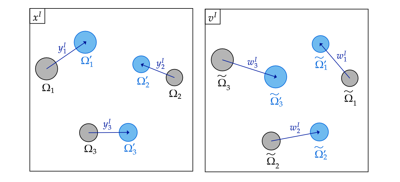
Figure 1: (Left) Action of the unitary operator $\mathcal{U}_{1}[f]$ which translates the wavepackets by an amount $y_{j}$ and so shifts their domain of central support in position space according to $\Omega_{j}\mapsto\Omega_{j}+y_{j}$. (Right) Action of the unitary operator $\mathcal{U}_{1}[Y^{I}]$ which boosts the wavepackets by an amount $w_{j}$ and so shifts their domain of central support in momentum space according to $\widetilde{\Omega}_{j}\mapsto\widetilde{\Omega}_{j}+w_{j}$.

Because $\widetilde{\Omega}_{j}$ are disjoint, we may choose a function $f(v)$ that is linear on the domains $\widetilde{\Omega}_{j}$

$$f(v)|_{\widetilde{\Omega}_{j}}=y_{j}\cdot v,$$ (5.8)

where $y_{1},...,y_{n}\in\mathbb{R}^{9}$ are an arbitrary set of vectors. When $y_{j}$ are all the same, we may simply take $f(v)$ to be the globally-defined linear function $f(v)=y\cdot v$. According to Table 2, the corresponding charge is just the BFSS momentum operator $y\cdot P$ which infinitesimally translates all particles in the $y$ direction by the same amount. When the constants $y_{j}$ differ, however, the wavepackets get infinitesimally translated in different directions. For example, if we define the unitary operator, $\mathcal{U}_{a}[f],$ generated by the conserved charge $\mathcal{Q}[f]$ as

$$\mathcal{U}_{a}[f]=\exp(ia\hskip 1.0pt\mathcal{Q}[f])=\exp(ia\hskip 1.0pt\mathcal{Q}_{S}[f]+ia\hskip 1.0pt\mathcal{Q}_{H}[f]),$$ (5.9)

then we observe that the hard term in $\mathcal{U}_{a}[f]$ translates the $j^{\text{th}}$ particle according to $x_{j}\mapsto x_{j}+ay_{j}$. Meanwhile, the soft term – being proportional to a soft D0-brane creation operator – is responsible for creating a coherent state of soft D0-branes. Thus, we see how adding soft D0-branes can be secretly equivalent to translating the hard D0-branes.

Similarly, we may choose the function $Y^{I}(v)$ such that it is constant on the domains $\widetilde{\Omega}_{j}$

$$Y^{I}(v)|_{\widetilde{\Omega}_{j}}=w_{j}^{I},$$ (5.10)

where $w_{1},...,w_{n}\in\mathbb{R}^{9}$ are another arbitrary set of vectors. When $w_{j}$ are all the same, we may take $Y^{I}(v)$ to be the globally defined linear function $Y^{I}(v)=w^{I}$. According to Table 2, the corresponding charge is just the generator of Galilean boosts in the matrix model $w\cdot\mathcal{K}$ (see Section 6.4) which infinitesimally changes the velocity of particles by an amount $w$. When the constants $w_{j}$ differ, however, the wavepackets get infinitesimally boosted by different amounts. If we define the unitary operator, $\mathcal{U}_{a}[Y^{I}],$ generated by the conserved charge $\mathcal{Q}[Y^{I}]$ as

$$\mathcal{U}_{a}[Y^{I}]=\exp(ia\hskip 1.0pt\mathcal{Q}[Y^{I}])=\exp(ia\hskip 1.0pt\mathcal{Q}_{S}[Y^{I}]+ia\hskip 1.0pt\mathcal{Q}_{H}[Y^{I}]),$$ (5.11)

then we observe that the hard term in $\mathcal{U}_{a}[f]$ changes the velocity of the $j^{\text{th}}$ particle according to $v_{j}\mapsto v_{j}+aw_{j}$. The soft term is again responsible for creating a coherent state of soft D0-branes. Thus, we see how adding soft D0-branes can also be secretly equivalent to individually boosting the hard D0-branes by specified amounts. This is summarized in Figure 1.

Of course, one could choose even more complicated functions $f(v)$ and $Y^{I}(v)$ which will distort wavepackets of D0-branes in arbitrarily non-trivial ways. The cost of doing so is integrating the soft D0-brane creation operator against these functions and then including this particle as an asymptotic state in a scattering amplitude.

6 Asymptotic Symmetries in the BFSS Matrix Model

In this section, we will interpret the aforementioned conservation laws in terms of asymptotic symmetries. Our main finding is that the asymptotic symmetries associated to the 11d large diffeomorphisms of M-theory are manifested in the D0-brane quantum mechanics via the asymptotic symmetries of the metric and RR 1-form gauge field in type IIA string theory. We offer several complementary perspectives and non-trivial consistency checks of this conclusion. Along the way, we find explicit expressions for the hard charges $\mathcal{Q}_{H}$ in terms of $N\times N$ matrix degrees of freedom.

6.1 Coupling BFSS to a Background 11d Metric

BFSS gives a dual description of M-theory with flat space metric, $\eta_{\mu\nu}$. We begin by briefly reviewing how the BFSS matrix model is deformed when one instead considers M-theory with a weakly curved background 11d metric, $\eta_{\mu\nu}+g_{\mu\nu}$, where $g_{\mu\nu}$ is independent of the coordinate $x^{-}$ parametrizing the compact direction. In a series of papers on D0-brane quantum mechanics, Taylor and Van Raamsdonk have argued that in the presence of such a background field, the BFSS action gets modified by the following interaction term [15, 56]

$$S_{\text{int}}[g_{\mu\nu}]=\frac{1}{2}\int dt~{}\sum_{m=0}^{\infty}\frac{1}{m!}\big{(}\partial_{I_{1}}\cdots\partial_{I_{m}}g_{\mu\nu}\big{)}T^{\mu\nu(I_{1}\cdots I_{m})}.$$ (6.1)

Here, $\partial_{I_{1}}\cdots\partial_{I_{m}}g_{\mu\nu}$ is a time-dependent coupling constant constructed from the background field, $g_{\mu\nu}$, and does not depend on the $N\times N$ matrix degrees of freedom. In particular, it is defined as the Taylor expansion of the 11d fields about the spatial origin in the transverse directions $x^{I}=0$

$$\partial_{I_{1}}\cdots\partial_{I_{m}}g_{\mu\nu}(t)=\frac{\partial}{\partial x^{I_{1}}}\cdots\frac{\partial}{\partial x^{I_{m}}}g_{\mu\nu}(x^{+},x^{I})\Big{|}_{x^{I}=0,~{}x^{+}=t}.$$ (6.2)

By contrast, $T^{\mu\nu}$ is the matrix theory stress-energy tensor and $T^{\mu\nu(I_{1}\cdots I_{m})}$ are its multipole moments. They are built out of the $N\times N$ matrix degrees of freedom, but have no background dependence. Furthermore, the stress-energy tensor satisfies the following conservation equation [57, 15, 56]

$$\partial_{0}T^{+\nu(I_{1}\cdots I_{m})}=T^{I_{1}\nu(I_{2}\cdots I_{m})}+\cdots+T^{I_{m}\nu(I_{1}\cdots I_{m-1})}.$$ (6.3)

We will need explicit expressions for a few components of the stress-energy tensor. In particular

$$\begin{split}T^{++}&=\frac{1}{R}\hskip 2.0pt\text{STr}\big{(}\mathds{1}\big{)}\\ T^{+I}&=\frac{1}{R}\hskip 2.0pt\text{STr}\big{(}\partial_{t}X^{I}\big{)}\\ T^{+-}&=\frac{1}{R}\hskip 2.0pt\text{STr}\Big{(}\frac{1}{2}\partial_{t}X^{I}\partial_{t}X^{I}-\frac{1}{4}[X^{I},X^{J}][X^{I},X^{J}]+\frac{1}{2}\Psi^{\alpha}\Gamma^{I}_{\alpha\beta}[X^{I},\Psi^{\beta}]\Big{)},\end{split}$$ (6.4)

where “STr” denotes the symmetrized trace of a product of matrices. The multipole moments of the matrix model stress-energy tensor are related to the zeroth order moments according to

$$T^{\mu\nu(I_{1}\cdots I_{m})}=\text{Sym}(T^{\mu\nu};X^{I_{1}},\cdots,X^{I_{m}})+T^{\mu\nu(I_{1}\cdots I_{m})}_{\text{fermion}},$$ (6.5)

where the first term denotes that we should insert the bosonic matrices, $X^{I}$, in the symmetrized traces considered in Equation (6.4) and the second term gives additional contributions to the multiple moments containing the fermions, $\Psi^{\alpha}.$ In particular, we will need the expressions

$$\begin{split}T^{++(J)}_{\text{fermion.}}&=0\\ T^{+I(J)}_{\text{fermion.}}&=\frac{1}{8R}\text{Tr}\big{(}\Psi^{\alpha}\Gamma^{[IJ]}_{\alpha\beta}\Psi^{\beta}\big{)}\\ T^{+-(J)}_{\text{fermion}}&=\frac{1}{16R}\text{Tr}\big{(}\Psi^{\alpha}[X^{K},X^{L}]\Gamma^{[KLJ]}_{\alpha\beta}\Psi^{\beta}+2i\Psi^{\alpha}\partial_{t}X^{K}\Gamma^{[KJ]}_{\alpha\beta}\Psi^{\beta}\big{)}.\end{split}$$ (6.6)

6.2 Asymptotic Symmetries in BFSS

Now, we will consider a setup where the 11d metric is pure gauge and related to the flat metric by an infinitesimal diffeomorphism generated by the vector field $\xi_{\mu}$

$$g_{\mu\nu}=\partial_{\mu}\xi_{\nu}+\partial_{\nu}\xi_{\mu}.$$ (6.7)

Moreover, we will study the situation where the gauge parameter $\xi_{\mu}$ is non-vanishing on $\mathcal{I}^{\pm}$ and is given by an expression of the form (3.11). It is known that in quantum field theory, a large diffeomorphism like this only affects one’s action up to a possible boundary term. Such a boundary term is precisely the conserved charge $Q[\xi_{\mu}]$ described in Equations (3.7) and (3.10).

In the case of D0-brane quantum mechanics, the same effect miraculously appears. We begin by considering $S_{\text{int}}[\partial_{\mu}\xi_{\nu}+\partial_{\nu}\xi_{\mu}]$. One may use the conservation equation to integrate this expression by parts. The resulting action can be written as the integral of a total derivative; therefore, it reduces to the following boundary term

$$S_{\text{int}}[\partial_{\mu}\xi_{\nu}+\partial_{\nu}\xi_{\mu}]=\sum_{m=0}^{\infty}\frac{1}{m!}\big{(}\partial_{I_{1}}\cdots\partial_{I_{m}}\xi_{\mu})T^{+\mu(I_{1}\cdots I_{n})}\bigg{|}_{-\infty}^{+\infty}.$$ (6.8)

As such, we may define the candidate incoming conserved charge, $\mathcal{Q}_{H}^{\text{in}}[\xi_{\mu}]$, by

$$\mathcal{Q}_{H}^{\text{in}}[\xi_{\mu}]=\sum_{m=0}^{\infty}\frac{1}{m!}\big{(}\partial_{I_{1}}\cdots\partial_{I_{m}}\xi_{\mu})T^{+\mu(I_{1}\cdots I_{n})}\bigg{|}_{-\infty}.$$ (6.9)

The candidate outgoing conserved charge is defined analogously. One can only recover the hard part of the conserved charge because $g_{\mu\nu}$ is a non-dynamical background field in this formalism.

6.3 Relation to RR 1-form and 10d Metric

In [32], we have argued that the soft theorem in the BFSS matrix model may be understood from the lens of studying asymptotic symmetries of the background RR 1-form gauge field, $A_{\mu},$ in type IIA string theory. This was originally noticed because the term $N_{j}/R$ appearing in the soft theorem is exactly the $U(1)$ charge of a stack of D0-branes under $A_{\mu}.$

In the previous section, we have argued that the asymptotic symmetries of M-theory are related to large diffeomorphisms of the 11d graviton field $g_{\mu\nu}$. These two perspectives reconcile because the 11d graviton field is broken down to a 10d metric perturbation, $h_{\mu\nu}$, a RR 1-form gauge field, $A_{\mu},$ and a dilaton, $\phi$ when compactified – thus, asymptotic symmetries of M-theory are at least partially manifested in the asymptotic symmetries of $A_{\mu}$. The full 11d gravitational asymptotic symmetry group of M-theory is manifested in D0-brane quantum mechanics dual via the asymptotic symmetries of $h_{\mu\nu}$ and $A_{\mu}$.

To see this, we note that the discrete lighcone quantization of M-theory may be viewed as a particular limit of so-called $\widehat{\text{M}}$-theory, which is just ordinary M-theory compactified along the $x^{10}$ direction with radius of compactification $R_{c}.$ $\widehat{\text{M}}$-theory is related to the DLCQ of M-theory via a large boost in the $x^{10}$ direction with parameter $\gamma=\sqrt{R^{2}/2R^{2}_{c}+1}$ followed by taking the $R_{c}\rightarrow 0$ limit [16]. The background metric perturbation in these two theories are similarly related by a large boost, so the Lorentz transformation with parameter $\gamma$ maps $g_{\mu\nu}\mapsto\widehat{g}_{\mu\nu}$ and also $\xi_{\mu}\mapsto\widehat{\xi}_{\mu}$ relating the 11d gauge parameters for the background metric in the two descriptions. The $R_{c}\rightarrow 0$ limit of $\widehat{\text{M}}$-theory is just type IIA string theory with background fields [56]

$$\begin{split}h_{\mu\nu}&=\widehat{g}_{\mu\nu}+\frac{1}{2}\widehat{g}_{10\hskip 1.0pt10}\hskip 30.0ptA_{\mu}=\widehat{g}_{10\hskip 1.0pt\mu}\hskip 30.0pt\phi=\frac{3}{4}\widehat{g}_{10\hskip 1.0pt10}.\end{split}$$ (6.10)

Plugging in the expressions for $\widehat{g}_{\mu\nu}$ in terms of $g_{\mu\nu}$ yields expressions for the type IIA background field in terms of the original 11d metric (see [56])

If $g_{\mu\nu}$ is pure gauge, then $\widehat{g}_{\mu\nu}$ is similarly pure gauge, and the 10-dimensional type IIA fields will necessarily be pure gauge as well

$$h_{\mu\nu}=\partial_{\mu}\zeta_{\nu}+\partial_{\nu}\zeta_{\mu}\hskip 30.0ptA_{\mu}=\partial_{\mu}\lambda,$$ (6.11)

for some 10d gauge parameters $(\zeta_{\mu},\lambda)$. One can read off expressions for these gauge parameters in terms of the 11d gauge parameter, $\widehat{\xi}_{\mu}$ by plugging $\widehat{g}_{\mu\nu}=\partial_{\mu}\widehat{\xi}_{\nu}+\partial_{\nu}\widehat{\xi}_{\mu}$ into Equation (6.10).

$$\begin{split}\zeta_{0}&=\widehat{\xi}_{0}=\frac{1}{\alpha\sqrt{2}}\xi_{+}-\frac{\alpha}{\sqrt{2}}\xi_{-}\\ \zeta_{I}&=\widehat{\xi}_{I}=\xi_{I}\color[rgb]{1,1,1}\bigg{|}\color[rgb]{0,0,0}\\ \lambda&=\widehat{\xi}_{10}=\frac{1}{\alpha\sqrt{2}}\xi_{+}-\frac{\alpha}{\sqrt{2}}\xi_{-}~{},\end{split}$$ (6.12)

where we have also related the 11d gauge parameter of $\widehat{\text{M}}$-theory, $\widehat{\xi}_{\mu}$, to the 11d gauge parameter of M-theory, $\xi_{\mu}$, via the aforementioned Lorentz boost. This expression depends on the parameter $\alpha\approx R_{s}/\sqrt{2}R\rightarrow 0$. Though several terms in Equation (6.12) appear to be either vanishing or divergent in the $\alpha\rightarrow 0$ limit, they always appear in finite combinations due to an additional rescaling of parameters relating type IIA string theory to the BFSS action (see [56, 16]).

In [32], we have shown that one may construct a hard charge associated to the 10d gauge field, $\mathcal{Q}_{H}[\lambda]$, via a similar integration by parts procedure as the one outlined in Section 6.2. Moreover, this charge reproduces Equation (5.2) when asymptotic states assume the form given by Equation (2.4). One can construct a similar charge for the 10d metric, $\mathcal{Q}^{\text{in}}_{H}[\zeta^{\mu}].$ This gives additional evidence that the asymptotic symmetries of the 11d metric are encoded in the D0-brane quantum mechanics picture through the asymptotic symmetries of $h_{\mu\nu}$ and $A_{\mu}$ in type IIA string theory and further bolsters the claim that $\mathcal{Q}^{\text{in}}_{H}[\xi^{\mu}]$ defined in Equation (6.9) is the correct definition for the hard charge in the matrix model. In [32], we also showed how adding a soft D0-brane can be viewed as turning on a background, pure gauge $A_{\mu}$ field – this formalism makes clear that it should be interpreted as turning on a background, pure gauge $g_{\mu\nu}$ field which decomposes into pure gauge IIA $A_{\mu}$ and $h_{\mu\nu}$ fields according to Equation (6.12).

6.4 Construction of Poincaré Generators in the Matrix Model

$\xi_{\mu}\partial^{\mu}$	M-theory: $Q_{H}[\xi^{\mu}]$	BFSS: $\mathcal{Q}_{H}[\xi^{\mu}]$
$\partial^{+}$	$P^{+}$	$T^{++}={\frac{N}{R}}$
$\partial^{I}$	$P^{I}$	$T^{+I}=\text{Tr}(P^{I})$
$\partial^{-}$	$P^{-}$	$T^{+-}=H_{\text{BFSS}}$
$x^{I}\partial^{J}-x^{J}\partial^{I}$	$J^{IJ}$	$T^{+J(I)}-T^{+I(J)}=\mathcal{J}^{IJ}$
$x^{+}\partial^{I}-x^{I}\partial^{+}$	$J^{+I}$	$-T^{++(I)}=\mathcal{K}^{I}$
$x^{-}\partial^{I}-x^{I}\partial^{-}$	$J^{-I}$	-
$x^{-}\partial^{+}-x^{+}\partial^{-}$	$J^{-+}$	-

Table 3: Correspondence between M-theory Poincaré generators and the dual BFSS generators which are defined by $\mathcal{Q}_{H}[\xi^{\mu}]$ for various choices of $\xi^{\mu}.$

Equation (6.9) gives an explicit candidate for the hard charge, $\mathcal{Q}_{H}[\xi^{\mu}]$, in the BFSS matrix model associated to a large diffeomorphism in M-theory generated by the vector field $\xi^{\mu}\partial_{\mu}.$ As such, it is especially interesting to try to use $\mathcal{Q}_{H}[\xi^{\mu}]$ to reproduce the generators of global translations and Lorentz transformations in the matrix model in an effort to identify how the 11d Poincaré algebra is actually manifested in terms of the $N\times N$ matrix degrees of freedom.

In the M-theory picture, the conserved charges associated to global translations are the momentum operators $P^{+}$, $P^{I}$, and $P^{-}$. In the BFSS picture, we expect the corresponding charges to be $N/R$ (due to the fact that we are working in a sector of M-theory where $P^{+}=N/R$), the BFSS momentum operator $\text{Tr}(P^{I})$, and the BFSS Hamiltonian which generates time translations (and so plays a similar role to $P^{-}$ in the lightcone quantization of M-theory). We also expect the M-theory Lorentz generator $J^{IJ}$ to be dual to the generator of $SO(9)$ rotations in the matrix model

$$\mathcal{J}^{IJ}=\text{Tr}\big{(}P^{I}X^{J}-P^{J}X^{I}\big{)}+\frac{1}{8R}\text{Tr}\big{(}\Psi^{\alpha}\Gamma^{[IJ]}_{\alpha\beta}\Psi^{\beta}\big{)},$$ (6.13)

while the Lorentz generator $J^{+I}$ should be dual to the generator of Galilean boosts

$$\mathcal{K}^{I}={\frac{1}{R}}\text{Tr}(X^{I}).$$ (6.14)

It is encouraging to find that by plugging in appropriate choices of the vector field $\xi^{\mu}$ into $\mathcal{Q}_{H}[\xi^{\mu}]$, these expectations are exactly realized (see Table 3)!

Unfortunately, one cannot construct the dual description of the M-theory generators $J^{-I}$ and $J^{+-}$ using this technology. This is due to the fact that the background field formalism we have been employing is incompatible with vector fields $\xi^{\mu}\partial_{\mu}$ which vary non-trivially in the compact $x^{-}$ direction [15, 56]. We hope that a suitable modification of the above prescription will allow one to fully construct the $11d$ Lorentz generators using only the $N\times N$ matrix degrees of freedom.

Nevertheless, the correspondence between the symmetry generators of M-theory and those of BFSS afforded by this formalism is a heartening result and offers a non-trivial consistency check regarding how the asymptotic symmetries of M-theory are manifested in the matrix model dual.

7 Discussion

In this work, we examined how the soft theorems and infinitely many conserved charges associated to asymptotic symmetries in M-theory are manifested in the matrix model dual. In particular, we made a conjecture about the structure of scattering amplitudes among D0-brane bound states in the limit where the number of D0-branes in one particular bound state is dwarfed by the number of D0-branes in all others. While this conjecture was based on the original description of the BFSS duality, we presented a first-principle calculation of it by considering the BFSS scaling limit of D0-brane scattering amplitudes in type IIA string theory, thus providing a novel test of the BFSS duality in a completely new setting. We showed how this soft theorem implies that BFSS enjoys conservation laws associated to the counterpart of 11d supertranslation and superrotation symmetry in the M-theory picture – these conservation laws are only realized in the large $N$ limit of the matrix model, which is necessary for consistency with the gravity description. Moreover, we interpreted the infinite dimensional symmetry algebra of BFSS, which gives rise to these conservation laws, in terms of the asymptotic symmetries of the metric and RR 1-form gauge field of type IIA string theory, which appear as background fields. Finally, we showcased how these perspectives reconcile to provide a consistent understanding of 11d Lorentz symmetry in the matrix model. In particular, we have shown that BFSS scattering amplitudes exhibit the full 11d Poincaré symmetry of M-theory which emerges only in the large $N$ limit, a claim which has been long anticipated but never verified.

We hope that this project will also springboard future studies of the matrix model and the relationship between celestial holography and BFSS. Celestial holography provides a natural framework for studying the symmetries of flat space, and it would be interesting to see how these ideas are manifested in the matrix model [62, 63, 64, 65, 66, 67, 68, 69, 70, 71, 72]. For example, a $w_{1+\infty}$ holographic symmetry algebra associated to soft gravitons was recently identified [73, 74, 75, 76, 77, 78, 79, 80, 81, 82, 83]. It is known that the $SU(N)\subset U(N)$ part of the BFSS symmetry algebra tends to the $w_{1+\infty}$ algebra as $N\rightarrow\infty$ [75, 17]. It would be exciting to see if this concordance actually encodes a deep connection.

It would also be intriguing to investigate how these concepts are related to black holes in the matrix model. In particular, the soft theorem describes how an $\mathcal{O}(1)$ number of D0-branes can get dislodged in scattering amplitudes. This is remniscent of Hawking radiation wherein individual D0-branes are the Hawking quanta of a Schwartzchild black hole, which is a Boltzmann gas of $N$ D0-branes [84, 85, 86, 87]. For additional work relating BFSS to black holes, see [88, 89, 90, 91, 92, 93, 94, 95, 96, 97, 98].

Finally, this work leaves a number of interesting follow-up questions and calculations. For example, one might hope to give a worldline proof of the soft theorem using the matrix model Hamiltonian (2.2). Recovering the leading term $\propto\hskip 2.0ptN$ would complement the derivation provided in Appendix A and be a very interesting computation in its own right. One could also try to understand how the soft theorems associated to the gravitino and 3-form gauge field in 11d $\mathcal{N}=1$ supergravity are realized in BFSS. In this work, we have only discussed soft theorems for D0-branes in the matrix model whose polarization tensors correspond to gravitons in the M-theory description – examining soft theorems for the other particles in the supermultiplet will likely shed light on new symmetries of the matrix model which are only realized in the large $N$ limit. A better understanding of the compact direction and how one could use the formalism of Section 6 to construct explicit expressions for the complete set of Poincaré generators would also be desirable.

Appendix A A First-Principle Argument for the Soft Theorem in BFSS

In this Appendix, we provide a derivation that non-relativistic D0-brane scattering amplitudes obey the soft theorem given by Equation (4.1).

Soft Theorems and $S^{1}$ Compactification

We will begin by revisiting the soft graviton theorem in M-theory. This time, however, we will not consider the DLCQ of M-theory – rather, we will work with the more familiar quantization on hypersurfaces of constant time. The leading soft graviton theorem obeys the usual universal expression in the limit $\omega_{s}/\omega_{j}\rightarrow 0$ where the supergraviton momenta are parametrized by (2.5)

$$\mathcal{A}_{\text{M}}(q_{s}^{\mu},\varepsilon;p_{1}^{\mu},...,p_{n}^{\mu})=\Big{[}\mathcal{S}^{(-1)}+\cdots\Big{]}\mathcal{A}_{\text{M}}(p_{1}^{\mu},...,p_{n}^{\mu}),$$ (A.1)

where

$$\mathcal{S}^{(-1)}=\frac{\kappa}{2}\hskip 2.0pt\varepsilon_{\mu\nu}\sum_{j=1}^{n}\eta_{s}\eta_{j}\frac{p_{j}^{\mu}p_{j}^{\nu}}{q_{s}\cdot p_{j}}.$$ (A.2)

For the moment, we will only focus on the leading term in the soft expansion.

Next, we compactify on a spatial circle with radius of compactification $R_{c}$ (in the $x^{10}$ direction, for simplicity). Now the momentum in the compact direction is quantized

$$p^{10}_{j}=\frac{\omega_{j}}{\sqrt{2}}(1-v_{j}^{2})=\frac{N_{j}}{R_{c}}\hskip 30.0pt\text{and}\hskip 30.0ptq^{10}_{s}=\frac{\omega_{s}}{\sqrt{2}}(1-v_{s}^{2})=\frac{N_{s}}{R_{c}}.$$ (A.3)

While the above expression is universal in theories of gravity in flat space, it is a priori unclear whether the leading soft term $\mathcal{S}^{(-1)}$ is corrected upon compactification. For example, the leading soft term may be spoiled by $\mathcal{O}(1/R_{c})$ corrections. In [50], it was argued that such terms do not arise when the soft particle is a KK zero-mode, with momentum $q^{10}_{s}=0.$ One may also demonstrate that one need not worry about any such corrections, more generally. Thus, the expression (A.2) holds for theories of gravity even when they have a compactified dimension.

It will be convenient to rewrite the leading soft term, $\mathcal{S}^{(-1)}$ in terms of the quantum numbers $(\omega_{j},v_{j}^{I})$,

$$\mathcal{S}^{(-1)}=-2\kappa\sum_{j=1}^{n}\eta_{s}\eta_{j}\frac{\omega_{j}}{\omega_{s}}\frac{e_{IJ}(v_{s}-v_{j})^{I}(v_{s}-v_{j})^{J}}{(v_{s}-v_{j})^{2}}.$$ (A.5)

At this point, we should still view the scattering amplitude as occurring in an 11-dimensional theory of gravity with one compactified dimension. The only constraint on the parameters $(\omega_{j},v_{j}^{I})$ is the quantization condition (A.3).

Soft Theorems for D0-Branes in Type IIA String Theory

Because the leading soft term retains its universal form even when one of the directions is compactified, it follows that soft theorems may be applied to KK modes as well. Specifically, we will consider a situation where the soft particle has non-zero KK momentum, $q^{10}_{s}=N_{s}/R_{c}.$ The soft limit now reads

$$\frac{\omega_{s}}{\omega_{j}}=\frac{N_{s}}{N_{j}}\frac{1-v_{j}^{2}}{1-v_{s}^{2}}\rightarrow 0.$$ (A.6)

We see that the limit $N_{s}/N_{j}\rightarrow 0$ (keeping the parameters $v_{s},v_{j}$ fixed) recovers the soft limit for KK modes.

Inserting Equation (A.6) into the soft theorem (A.5), we find the following soft theorem associated to scattering of graviton KK modes in the 10-dimensional type IIA string theory. Now, the parameter $N_{j}$ labels the KK mode of the corresponding particle,

$$\mathcal{S}^{(-1)}=-2\kappa\sum_{j=1}^{n}\eta_{s}\eta_{j}\frac{N_{s}}{N_{j}}\frac{1-v_{j}^{2}}{1-v_{s}^{2}}\frac{e_{IJ}(v_{s}-v_{j})^{I}(v_{s}-v_{j})^{J}}{(v_{s}-v_{j})^{2}}.$$ (A.7)

The KK modes are just D0-brane bound states where the integer $N_{j}$ labels the number of D0-branes in a particular bound state. Thus, we have recovered a soft theorem for D0-branes where the soft limit is precisely $N_{s}/N_{j}\rightarrow 0$, just as it was in the BFSS case.

Soft Theorem for Non-Relativistic D0-Branes: The BFSS Limit

Up to this point, we have been studying D0-brane scattering in IIA where the D0-branes may be relativistic. The BFSS matrix model concerns only non-relativistic D0-brane dynamics, however. Fortunately, it is known how to rescale the parameters in type IIA string theory to recover the BFSS action for these non-relativistic D0-branes [16]. Indeed, BFSS can be viewed as a particular scaling limit of weakly coupled type IIA string theory, and the scattering amplitudes of D0-brane bound states in the two descriptions should agree by definition – this agreement is at the heart of our argument.

For the leading soft term, $\mathcal{S}^{(-1)}$, of Equation (A.7) this rescaling amounts to taking the non-relativistic limit $v_{j}\mapsto\varepsilon v_{j}$ where $\varepsilon\rightarrow 0.$ In this non-relativistic limit, Equation (A.7) reads

$$\mathcal{S}_{\text{BFSS}}^{(-1)}=-2\kappa\sum_{j=1}^{n}\eta_{s}\eta_{j}\frac{N_{s}}{N_{j}}\frac{e_{IJ}(v_{s}-v_{j})^{I}(v_{s}-v_{j})^{J}}{(v_{s}-v_{j})^{2}}.$$ (A.8)

This is precisely the form for the leading soft theorem that we previously conjectured for D0-brane scattering in BFSS via the duality dictionary! A similar computation may be considered to show equality at subleading order, $\mathcal{S}^{(0)}.$ Though this calculation did not involve working with the $N\times N$ matrix degrees of freedom familiar to BFSS, it is still a bona fide non-relativistic D0-brane calculation in type IIA string theory and, thus, gives strong evidence that the BFSS matrix model enjoys the soft theorems discussed in Section 4.1. Nevertheless, a direct computation using the D0-brane worldline Hamiltonian (2.2) would be illuminating.

Note that while this argument also relies on the equivalence between M-theory compactified on a small circle and type IIA string theory, it is qualitatively different from Seiberg’s classic argument that the DLCQ of M-theory should be described by BFSS [16]. The latter invokes an infinitely large Lorentz boost which relates DLCQ M-theory to $\widehat{\text{M}}$-theory (see Section 6.3) compactified on a small spatial circle (and so their amplitudes, being Lorentz invariant, might plausibly agree). This is not the spirit of our argument – we instead give a first-principle computation of the relevant amplitudes in spatially compactified $\widehat{\text{M}}$-theory without discussing amplitudes in DLCQ M-theory at all. This requires us to take great care in showing that any possible $\mathcal{O}(1/R_{c})$ corrections vanish for the particular case of soft theorems but allows us to avoid discussing any thorny details about possible convergence issues when infinitely large boosts are involved. Once we know the relationship between D0-brane amplitudes with a soft D0-brane and those without one in IIA, taking the BFSS limit wherin the external D0-branes are non-relativistic recovers BFSS amplitudes tautologically.

Appendix B Derivation of Conservation Laws in the Matrix Model

In this appendix, we will detail how the leading and subleading soft theorem in the matrix model implies the conservation of infinitely many charges $\mathcal{Q}[f]$ and $\mathcal{Q}[Y^{I}]$ given in Sections 5.1 and 5.2.

Shadow Transform Details

The heart of this argument relies on an integral transformation known as the shadow transform. We define the shadow transform on the D0-brane creation operator $\mathcal{G}_{IJ}^{\text{in}\dagger}(N_{s},v_{s})$ as

$$\widetilde{\mathcal{G}}^{\hskip 1.0pt\text{in},\dagger}_{\Delta,IJ}(N_{s},v_{s})=\mathcal{N}_{\Delta}~{}\delta^{\{K}_{\{I}\delta^{L\}}_{J\}}\int d^{9}w_{s}~{}\frac{\mathcal{I}_{KM}(v_{s}-w_{s})\mathcal{I}_{LN}(v_{s}-w_{s})}{(v_{s}-w_{s})^{2(9-\Delta)}}~{}\mathcal{G}_{MN}^{\hskip 1.0pt\text{in}\dagger}(N_{s},u_{s}),$$ (B.1)

where $\{\cdot,\cdot\}$ denotes the symmetric traceless projection on the given indices, $\mathcal{I}_{IJ}(v)=\delta_{IJ}-2v_{I}v_{J}/v^{\hskip 1.5pt2}$ is the inversion tensor familiar from conformal field theory, and $\mathcal{N}_{\Delta}$ is a normalization coefficient which regulates the integral

$$\mathcal{N}_{\Delta}=\frac{(\Delta+1)(10-\Delta)\Gamma(\Delta)\Gamma(9-\Delta)}{\pi^{9}(\Delta-1)(8-\Delta)\Gamma(\tfrac{9}{2}-\Delta)\Gamma(\Delta-\tfrac{9}{2})}.$$ (B.2)

Notice that applying the shadow transform to the D0-brane creation operator $\mathcal{G}_{IJ}^{\text{in}\dagger}(N_{s},v_{s})$ does not affect the number of D0-branes added to the state – it will always be $N_{s}$. Rather, it simply smears the velocity of the D0-branes which are added against some kernel. This shadow transform is especially useful in celestial conformal field theory and plays a large role in demonstrating that soft theorems are equivalent to conservation laws in general gauge and gravitational theories.

There will be two particular shadow transforms that we need to extract details about the leading and subleading soft theorems and to derive their associated conservation laws. In particular, we define the leading shadow transformed creation operator and subleading shadow transformed creation operator respectively as

$$\begin{split}&\textbf{leading:}\hskip 42.0pt\widetilde{\mathcal{G}}^{\hskip 1.0pt(-1)\hskip 1.0pt\text{in}\dagger}_{IJ}(N_{s},v_{s})=\lim_{\Delta\rightarrow\hskip 1.0pt1}~{}\widetilde{\mathcal{G}}^{\hskip 1.0pt\text{in}\dagger}_{\Delta,IJ}(N_{s},v_{s})\\ &\textbf{subleading:}\hskip 30.0pt\widetilde{\mathcal{G}}^{\hskip 1.0pt(0)\hskip 1.0pt\text{in}\dagger}_{IJ}(N_{s},v_{s})=\lim_{\Delta\rightarrow\hskip 1.0pt0}~{}\widetilde{\mathcal{G}}^{\hskip 1.0pt\text{in}\dagger}_{\Delta,IJ}(N_{s},v_{s}).\end{split}$$ (B.3)

Shadow transforms for the outgoing creation operators may be defined in an identical way.

Derivation of Leading-Order Conserved Charges

We begin by restating the soft theorem in the matrix model (Equation (4.4))

$$\begin{split}\frac{N_{s}}{R}\langle\text{out}|\frac{1}{2}\Big{[}\mathcal{G}^{\hskip 1.0pt(-1)\hskip 1.0pt\text{out}}_{IJ}(&N_{s},v_{s})-\mathcal{G}^{\hskip 1.0pt(-1)\hskip 1.0pt\text{in}\hskip 1.0pt\dagger}_{IJ}(N_{s},v_{s})\Big{]}|\text{in}\rangle\\ &=\frac{\kappa}{2}\bigg{[}-2\sum_{j=1}^{n}\eta_{j}\frac{N_{j}}{R}\frac{(v_{s}-v_{j})^{I}(v_{s}-v_{j})^{J}}{(v_{s}-v_{j})^{2}}\bigg{]}\langle\text{out}|\text{in}\rangle+\mathcal{O}\Big{(}\frac{N_{s}}{R}\Big{)}\\ &=\frac{\kappa}{2}\bigg{[}-2\sum_{j=1}^{n}\eta_{j}\frac{N_{j}}{R}\frac{(v_{s}-v_{j})^{I}(v_{s}-v_{j})^{J}}{(v_{s}-v_{j})^{2}}\bigg{]}\langle\text{out}|\text{in}\rangle+\mathcal{O}\Big{(}\frac{1}{N}\Big{)},\end{split}$$ (B.4)

where we have used the fact that $R\sim N$ and $N_{s}\sim\mathcal{O}(1)$ to write $\mathcal{O}(N_{s}/R)$ and $\mathcal{O}(1/N)$ on the last line. It has been shown one may apply the shadow transform to both sides of this expression to find [27]

$$\begin{split}\frac{N_{s}}{4R}\langle\text{out}|\frac{1}{2}\partial_{v_{s}^{I}}\partial_{v_{s}^{J}}\Big{[}\widetilde{\mathcal{G}}^{\hskip 1.0pt(-1)\hskip 1.0pt\text{out}}_{IJ}(&N_{s},v_{s})-\widetilde{\mathcal{G}}^{\hskip 1.0pt(-1)\hskip 1.0pt\text{in}\hskip 1.0pt\dagger}_{IJ}(N_{s},v_{s})\Big{]}|\text{in}\rangle\\ &=\frac{\kappa}{2}\sum_{j=1}^{n}\eta_{j}\frac{N_{j}}{R}\delta^{(9)}(v_{s}-v_{j})\langle\text{out}|\text{in}\rangle+\mathcal{O}\Big{(}\frac{1}{N}\Big{)}.\end{split}$$ (B.5)

Though the right hand side of this expression has singular behavior when $v_{s}=v_{j}$, we may smooth out this feature by integrating against an arbitrary function $f(v_{s}),$

$$\begin{split}\frac{N_{s}}{8R}\langle\text{out}|\int d^{9}v_{s}~{}f(v_{s})\partial_{v_{s}^{I}}\partial_{v_{s}^{J}}\Big{[}\widetilde{\mathcal{G}}^{\hskip 1.0pt(-1)\hskip 1.0pt\text{out}}_{IJ}(&N_{s},v_{s})-\widetilde{\mathcal{G}}^{\hskip 1.0pt(-1)\hskip 1.0pt\text{in}\hskip 1.0pt\dagger}_{IJ}(N_{s},v_{s})\Big{]}|\text{in}\rangle\\ &=\frac{\kappa}{2}\sum\eta_{j}\frac{N_{j}}{R}f(v_{j})\langle\text{out}|\text{in}\rangle+\mathcal{O}\Big{(}\frac{1}{N}\Big{)}.\end{split}$$ (B.6)

Moving the first term on the right-hand side to the left hand side yields an expression that vanishes as $\mathcal{O}(1/N)$. An immediate consequence is that the charges $\mathcal{Q}^{\text{in}}[f]$ and $\mathcal{Q}^{\text{out}}[f]$ defined in Equation (5.2) satisfy the conservation law

$$\langle\text{out}|\Big{(}\mathcal{Q}^{\text{out}}[f]-\mathcal{Q}^{\text{in}}[f]\Big{)}|\text{in}\rangle=\mathcal{O}\Big{(}\frac{1}{N}\Big{)}.$$ (B.7)

Derivation of Subleading-Order Conserved Charges

The first set of conserved charges, $\mathcal{Q}[f]$, were derived by considering the leading term in the soft expansion only. To derive a second set, $\mathcal{Q}[Y^{I}]$, we wish to isolate the subleading term in the soft expansion. One could do this by applying the following projection operator $(1+\tfrac{N_{s}}{R}\partial_{N_{s}/R})$ to the soft expansion – this would project out the leading soft term but preserve the subleading corrections. However, $N_{s}\in\mathbb{N}$ is quantized, so taking derivatives is ill-defined. Instead, we will approximate this derivative operator by finite differences. Upon doing so, the projection operator reads

$$\mathbb{P}\hskip 1.0pt\mathcal{G}_{IJ}^{\hskip 1.0pt\text{in}\hskip 1.0pt\dagger}(N_{s},v_{s})=\mathcal{G}_{IJ}^{\hskip 1.0pt\text{in}\hskip 1.0pt\dagger}(N_{s},v_{s})+N_{s}\Big{[}\mathcal{G}_{IJ}^{\hskip 1.0pt\text{in}\hskip 1.0pt\dagger}(N_{s}+1,v_{s})-\mathcal{G}_{IJ}^{\hskip 1.0pt\text{in}\hskip 1.0pt\dagger}(N_{s},v_{s})\Big{]}.$$ (B.8)

If we write the soft theorem schematically as

$$\langle\text{out}|\frac{1}{2}\Big{[}\mathcal{G}_{IJ}^{\hskip 1.0pt\text{out}}(N_{s},v_{s})-\mathcal{G}_{IJ}^{\hskip 1.0pt\text{in}\hskip 1.0pt\dagger}(N_{s},v_{s})\Big{]}\text{in}\rangle=\frac{N_{j}}{N_{s}}\mathcal{S}^{(-1)}\langle\text{out}|\text{in}\rangle+\mathcal{S}^{(0)}\langle\text{out}|\text{in}\rangle+\mathcal{O}\Big{(}\frac{1}{N}\Big{)},$$ (B.9)

one may quickly verify the following relation among the projected soft D0-brane creation operators

$$\begin{split}\langle\text{out}|\frac{1}{2}\Big{[}\mathbb{P}\hskip 1.0pt\mathcal{G}_{IJ}^{\hskip 1.0pt\text{out}}(&N_{s},v_{s})-\mathbb{P}\hskip 1.0pt\mathcal{G}_{IJ}^{\hskip 1.0pt\text{in}\hskip 1.0pt\dagger}(N_{s},v_{s})\Big{]}\text{in}\rangle\\ &=\mathcal{S}^{(-1)}\bigg{(}\frac{N_{j}}{N_{s}^{2}}\frac{1}{1+1/N_{s}}\bigg{)}\langle\text{out}|\text{in}\rangle+\mathcal{S}^{(0)}\langle\text{out}|\text{in}\rangle+\mathcal{O}\Big{(}\frac{1}{N}\Big{)}\\ &=\mathcal{S}^{(0)}\langle\text{out}|\text{in}\rangle+\mathcal{O}\Big{(}\frac{1}{N}\Big{)}.\end{split}$$ (B.10)

Thus, we have projected out the leading piece, as desired. There is a slight technical complication, however, in that we must take $N_{s}\sim N^{\alpha}$ for some $\alpha\in(\tfrac{1}{2},1)$ so that the term $N_{j}/N_{s}^{2}(1+1/N_{s})$ vanishes in the large $N$, M-theory limit. While this term won’t quite vanish as fast as $1/N$, it does vanish in the M-theory limit, so we group it into the $\mathcal{O}(1/N)$ corrections.

It has been shown that one may apply the shadow transform to both sides of this expression to find [54].

$$\begin{split}\langle\text{out}|\frac{1}{2}\Big{[}&\partial_{v_{s}^{I}}\hskip 1.0pt\mathbb{P}\hskip 2.0pt\widetilde{\mathcal{G}}^{\hskip 1.0pt(0)\hskip 1.0pt\text{out}}_{IJ}(N_{s},v_{s})-\partial_{v_{s}^{I}}\hskip 1.0pt\mathbb{P}\hskip 2.0pt\widetilde{\mathcal{G}}^{\hskip 1.0pt(0)\hskip 1.0pt\text{in}\hskip 1.0pt\dagger}_{IJ}(N_{s},v_{s})\Big{]}|\text{in}\rangle\\ &=\frac{\kappa}{2}\sum_{j=1}^{n}\eta_{j}\bigg{[}\delta^{(9)}(v_{s}-v_{j})\partial_{v_{j}^{J}}+\frac{i}{2}\partial_{v_{s}^{I}}\delta^{(9)}(v_{s}-v_{j})S_{j}^{IJ}+\frac{1}{9}\partial_{v_{s}^{J}}\delta^{(9)}(v_{s}-v_{j})\frac{N_{j}}{R}\partial_{N_{j}/R}\bigg{]}\\ &\hskip 70.0pt\times\langle\text{out}|\text{in}\rangle+\mathcal{O}\Big{(}\frac{1}{N}\Big{)},\end{split}$$ (B.11)

where the projection operator, $\mathbb{P}$, acts on the shadow transformed creation operator as in Equation (B.8). Now, we smear both sides of this expression against the arbitrary vector field, $Y^{I}$ to smooth over the delta-function singularity. The result is that the charges $\mathcal{Q}^{\text{in}}[Y^{I}]$ and $\mathcal{Q}^{\text{out}}[Y^{I}]$ defined in Equation (5.4) satisfy the conservation law

$$\langle\text{out}|\Big{(}\mathcal{Q}^{\text{out}}[Y^{I}]-\mathcal{Q}^{\text{in}}[Y^{I}]\Big{)}|\text{in}\rangle=\mathcal{O}\Big{(}\frac{1}{N}\Big{)},$$ (B.12)

where now the $\mathcal{O}(1/N)$ terms on the right hand side may vanish slightly slower than $1/N$, but still do vanish in the M-theory limit.

Appendix C Conservation Laws for 11d Poincaré Symmetry in M-Theory and BFSS

In this appendix, we will consider the conservation equations associated to the leading and subleading soft theorems in M-theory (Equation (3.13)) and BFSS (Equation (5.5))

$$\begin{split}\textbf{M-theory:}&\hskip 40.0pt\langle\text{out}|\Big{(}Q^{\text{out}}[f,Y^{I}]-Q^{\text{in}}[f,Y^{I}]\Big{)}|\text{in}\rangle=0\\ \textbf{BFSS:}&\hskip 40.0pt\langle\text{out}|\Big{(}\mathcal{Q}^{\text{out}}[f,Y^{I}]-\mathcal{Q}^{\text{in}}[f,Y^{I}]\Big{)}|\text{in}\rangle=\mathcal{O}\Big{(}\frac{1}{N}\Big{)}.\end{split}$$ (C.1)

As discussed in Section 5.3, for several choices of functions $(f,Y^{I})$ the conservation laws reduce to simple expressions. In the remainder of this appendix, we provide these expressions and give their interpretations. These identities demonstrate that D0-brane scattering amplitudes in BFSS enjoy the full 11d Poincaré symmetry in the large $N$ limit.

For $f(v)=1$, $Y^{K}(v)\partial_{K}=0$,

$$\begin{split}&\hskip 52.0pt{\sum}_{j}\hskip 3.0pt\eta_{j}\omega_{j}\mathcal{A}_{\text{M}}=0\hskip 165.0pt(\text{conservation of $P^{+}$})\\ &\hskip 52.0pt{\sum}_{j}\hskip 3.0pt\eta_{j}{\frac{N_{j}}{R}}\mathcal{A}_{\text{BFSS}}=\mathcal{O}\Big{(}\frac{1}{N}\Big{)}\hskip 118.0pt(\text{conservation of D0-branes})\end{split}$$ (C.2)

For $f(v)=\sqrt{2}v^{I}$, $Y^{K}(v)\partial_{K}=0$,

$$\begin{split}&\hskip 57.0pt{\sum}_{j}\hskip 3.0pt\eta_{j}\sqrt{2}\omega_{j}v^{I}_{j}\mathcal{A}_{\text{M}}=0\hskip 140.0pt(\text{conservation of $P^{I}$})\\ &\hskip 57.0pt{\sum}_{j}\hskip 3.0pt\eta_{j}\sqrt{2}{\frac{N_{j}}{R}}v^{I}_{j}\mathcal{A}_{\text{BFSS}}=\mathcal{O}\Big{(}\frac{1}{N}\Big{)}\hskip 92.0pt(\text{conservation of momentum})\end{split}$$ (C.3)

For $f(v)=v^{\hskip 1.0pt2}$, $Y^{K}(v)\partial_{K}=0$,

$$\begin{split}&\hskip 35.0pt{\sum}_{j}\hskip 3.0pt\eta_{j}\omega_{j}v^{2}\mathcal{A}_{\text{M}}=0\hskip 155.0pt(\text{conservation of $P^{-}$})\\ &\hskip 35.0pt{\sum}_{j}\hskip 3.0pt\eta_{j}{\frac{N_{j}}{R}}v^{2}\mathcal{A}_{\text{BFSS}}=\mathcal{O}\Big{(}\frac{1}{N}\Big{)}\hskip 108.0pt(\text{conservation of energy)}\end{split}$$ (C.4)

For $f(v)=0$, $Y^{K}(v)\partial_{K}=-(v^{I}\partial_{J}-v^{J}\partial_{I})$,

$$\begin{split}&{\sum}_{j}\hskip 3.0pt\eta_{j}[-i(v_{j}^{I}\partial_{v_{j}^{J}}-v_{j}^{J}\partial_{v_{j}^{I}})+S_{j}^{IJ}]\mathcal{A}_{\text{M}}=0\hskip 52.0pt(\text{conservation of $J_{IJ}$})\\ &{\sum}_{j}\hskip 3.0pt\eta_{j}[-i(v_{j}^{I}\partial_{v_{j}^{J}}-v_{j}^{J}\partial_{v_{j}^{I}})+S_{j}^{IJ}]\mathcal{A}_{\text{BFSS}}=\mathcal{O}\Big{(}\frac{1}{N}\Big{)}\hskip 10.0pt(\text{$SO(9)$ Invariance})\end{split}$$ (C.5)

For $f(v)=0$, $Y^{K}(v)\partial_{K}=\frac{1}{\sqrt{2}}\partial_{I}$,

$$\begin{split}&\hskip 60.0pt\frac{1}{\sqrt{2}}{\sum}_{j}\hskip 3.0pt\eta_{j}i\partial_{v_{j}^{I}}\mathcal{A}_{\text{M}}=0\hskip 138.0pt(\text{conservation of $J_{-I}$})\\ &\hskip 59.0pt\frac{1}{\sqrt{2}}{\sum}_{j}\hskip 3.0pt\eta_{j}i\partial_{v_{j}^{I}}\mathcal{A}_{\text{BFSS}}=\mathcal{O}\Big{(}\frac{1}{N}\Big{)}\hskip 97.0pt(\text{Galilean boost invariance})\end{split}$$ (C.6)

For $f(v)=0$, $Y^{K}(v)\partial_{K}=v^{K}\partial_{K}$,

$$\begin{split}&\hskip 40.0pt{\sum}_{j}\hskip 3.0pt\eta_{j}i(v_{j}^{I}\partial_{v_{j}^{I}}-\omega_{j}\partial_{\omega_{j}})\mathcal{A}_{\text{M}}=0\hskip 90.0pt(\text{conservation of $J_{+-}$})\\ &\hskip 40.0pt{\sum}_{j}\hskip 3.0pt\eta_{j}i(v_{j}^{I}\partial_{v_{j}^{I}}-{\frac{N_{j}}{R}}\partial_{N_{j}/R})\mathcal{A}_{\text{BFSS}}=\mathcal{O}\Big{(}\frac{1}{N}\Big{)}\hskip 32.0pt(\text{new symmetry})\end{split}$$ (C.7)

For $f(v)=0$, $Y^{K}(v)\partial_{K}=\frac{1}{\sqrt{2}}(v^{2}\partial_{I}-2v^{I}v^{K}\partial_{K})$,

$$\begin{split}&\frac{1}{\sqrt{2}}{\sum}_{j}\hskip 3.0pt\eta_{j}[i(v_{j}^{2}\partial_{v_{j}^{I}}-2v_{j}^{I}v_{j}^{J}\partial_{v_{j}^{J}}+2v_{j}^{I}\omega_{j}\partial_{\omega_{j}})+2v_{j}^{J}S_{j}^{IJ}]\mathcal{A}_{\text{M}}=0\hskip 46.0pt(\text{conservation of $J_{+I}$})\\ &\frac{1}{\sqrt{2}}{\sum}_{j}\hskip 3.0pt\eta_{j}[i(v_{j}^{2}\partial_{v_{j}^{I}}-2v_{j}^{I}v_{j}^{J}\partial_{v_{j}^{J}})+2v_{j}^{I}{\frac{N_{j}}{R}}\partial_{N_{j}/R}+2v_{j}^{J}S_{j}^{IJ}]\mathcal{A}_{\text{BFSS}}=\mathcal{O}\Big{(}\frac{1}{N}\Big{)}\hskip 12.0pt(\text{new symmetry})\end{split}$$ (C.8)

Note that the BFSS conservation laws follow from Equation (5.5) which is a consequence of the soft theorems discussed in Section 4 and derived in Appendix A. It follows that these symmetries are actually manifested in the matrix model; our derivation does not presuppose the BFSS duality relation among scattering amplitudes. Note the striking similarity between the top and bottom lines of Equations (C.2)-(C.8). The BFSS conservation laws are nothing but the M-theory conservation laws after translating through the duality dictionary. This gives definitive evidence that BFSS scattering amplitudes enjoy 11$d$ Poincaré symmetry.

References

- [1] Steven Weinberg, “Infrared photons and gravitons,” Phys. Rev. 140, B516–B524 (1965)
- [2] Jacob D. Bekenstein, “Black holes and entropy,” Phys. Rev. D 7, 2333–2346 (1973)
- [3] T. Banks, W. Fischler, S. H. Shenker, and L. Susskind, “M theory as a matrix model: A conjecture,” Phys. Rev. D 55, 5112–5128 (Apr 1997), https://link.aps.org/doi/10.1103/PhysRevD.55.5112
- [4] Leonard Susskind, “Another conjecture about M(atrix) theory,” (4 1997), arXiv:hep-th/9704080
- [5] Ashoke Sen, “D0-branes on T**n and matrix theory,” Adv. Theor. Math. Phys. 2, 51–59 (1998), arXiv:hep-th/9709220
- [6] Joseph Polchinski, “M theory and the light cone,” Prog. Theor. Phys. Suppl. 134, 158–170 (1999), arXiv:hep-th/9903165
- [7] Washington Taylor, “M(atrix) Theory: Matrix Quantum Mechanics as a Fundamental Theory,” Rev. Mod. Phys. 73, 419–462 (2001), arXiv:hep-th/0101126
- [8] D. Bigatti and Leonard Susskind, “Review of matrix theory,” NATO Sci. Ser. C 520, 277–318 (1999), arXiv:hep-th/9712072
- [9] Badis Ydri, “Review of M(atrix)-Theory, Type IIB Matrix Model and Matrix String Theory,” (8 2017), arXiv:1708.00734 [hep-th]
- [10] Yuji Okawa and Tamiaki Yoneya, “Multibody interactions of D particles in supergravity and matrix theory,” Nucl. Phys. B 538, 67–99 (1999), arXiv:hep-th/9806108
- [11] Yuji Okawa and Tamiaki Yoneya, “Equations of motion and Galilei invariance in D particle dynamics,” Nucl. Phys. B 541, 163–178 (1999), arXiv:hep-th/9808188
- [12] Katrin Becker and Melanie Becker, “A Two loop test of M(atrix) theory,” Nucl. Phys. B 506, 48–60 (1997), arXiv:hep-th/9705091
- [13] Katrin Becker, Melanie Becker, Joseph Polchinski, and Arkady A. Tseytlin, “Higher order graviton scattering in M(atrix) theory,” Phys. Rev. D 56, R3174–R3178 (1997), arXiv:hep-th/9706072
- [14] Daniel N. Kabat and Washington Taylor, “Linearized supergravity from matrix theory,” Phys. Lett. B 426, 297–305 (1998), arXiv:hep-th/9712185
- [15] Washington Taylor and Mark Van Raamsdonk, “Supergravity currents and linearized interactions for matrix theory configurations with fermionic backgrounds,” JHEP 04, 013 (1999), arXiv:hep-th/9812239
- [16] Nathan Seiberg, “Why is the matrix model correct?.” Phys. Rev. Lett. 79, 3577–3580 (1997), arXiv:hep-th/9710009
- [17] B. de Wit, J. Hoppe, and H. Nicolai, “On the Quantum Mechanics of Supermembranes,” Nucl. Phys. B 305, 545 (1988)
- [18] Jan de Boer and Sergey N. Solodukhin, “A Holographic reduction of Minkowski space-time,” Nucl. Phys. B 665, 545–593 (2003), arXiv:hep-th/0303006
- [19] Temple He, Prahar Mitra, and Andrew Strominger, “2D Kac-Moody Symmetry of 4D Yang-Mills Theory,” JHEP 10, 137 (2016), arXiv:1503.02663 [hep-th]
- [20] Sabrina Pasterski, Shu-Heng Shao, and Andrew Strominger, “Flat Space Amplitudes and Conformal Symmetry of the Celestial Sphere,” Phys. Rev. D 96, 065026 (2017), arXiv:1701.00049 [hep-th]
- [21] Andrew Strominger, “Lectures on the Infrared Structure of Gravity and Gauge Theory,” (3 2017), arXiv:1703.05448 [hep-th]
- [22] Ana-Maria Raclariu, “Lectures on Celestial Holography,” (7 2021), arXiv:2107.02075 [hep-th]
- [23] Sabrina Pasterski, “Lectures on celestial amplitudes,” Eur. Phys. J. C 81, 1062 (2021), arXiv:2108.04801 [hep-th]
- [24] Kevin Costello, Natalie M. Paquette, and Atul Sharma, “Top-Down Holography in an Asymptotically Flat Spacetime,” Phys. Rev. Lett. 130, 061602 (2023), arXiv:2208.14233 [hep-th]
- [25] Kevin Costello and Natalie M. Paquette, “Celestial holography meets twisted holography: 4d amplitudes from chiral correlators,” JHEP 10, 193 (2022), arXiv:2201.02595 [hep-th]
- [26] Arjun Kar, Lampros Lamprou, Charles Marteau, and Felipe Rosso, “A Matrix Model for Flat Space Quantum Gravity,” (8 2022), arXiv:2208.05974 [hep-th]
- [27] Daniel Kapec and Prahar Mitra, “Shadows and soft exchange in celestial CFT,” Phys. Rev. D 105, 026009 (2022), arXiv:2109.00073 [hep-th]
- [28] Stephan Stieberger, Tomasz R. Taylor, and Bin Zhu, “Celestial Liouville theory for Yang-Mills amplitudes,” Phys. Lett. B 836, 137588 (2023), arXiv:2209.02724 [hep-th]
- [29] Tomasz R. Taylor and Bin Zhu, “Celestial Supersymmetry,” (2 2023), arXiv:2302.12830 [hep-th]
- [30] Daniel Kapec, Vyacheslav Lysov, Sabrina Pasterski, and Andrew Strominger, “Semiclassical Virasoro symmetry of the quantum gravity -matrix,” JHEP 08, 058 (2014), arXiv:1406.3312 [hep-th]
- [31] Daniel Kapec, Vyacheslav Lysov, Sabrina Pasterski, and Andrew Strominger, “Higher-dimensional supertranslations and Weinberg’s soft graviton theorem,” Ann. Math. Sci. Appl. 02, 69–94 (2017), arXiv:1502.07644 [gr-qc]
- [32] Noah Miller, Andrew Strominger, Adam Tropper, and Tianli Wang, “Soft Gravitons in the BFSS Matrix Model,” (8 2022), arXiv:2208.14547 [hep-th]
- [33] Ulf H. Danielsson, Gabriele Ferretti, and Bo Sundborg, “D particle dynamics and bound states,” Int. J. Mod. Phys. A 11, 5463–5478 (1996), arXiv:hep-th/9603081
- [34] Daniel N. Kabat and Philippe Pouliot, “A Comment on zero-brane quantum mechanics,” Phys. Rev. Lett. 77, 1004–1007 (1996), arXiv:hep-th/9603127
- [35] C. Bachas, “D-brane dynamics,” Phys. Lett. B 374, 37–42 (1996), arXiv:hep-th/9511043
- [36] Savdeep Sethi and Mark Stern, “D-brane bound states redux,” Commun. Math. Phys. 194, 675–705 (1998), arXiv:hep-th/9705046
- [37] Gregory Moore, Nikita Nekrasov, and Samson Shatashvili, “D-particle bound states and generalized instantons,” Communications in Mathematical Physics 209, 77–95 (2000)
- [38] Piljin Yi, “Witten index and threshold bound states of d-branes,” Nuclear Physics B 505, 307–318 (1997)
- [39] Jan Plefka and Andrew Waldron, “On the quantum mechanics of M(atrix) theory,” Nucl. Phys. B 512, 460–484 (1998), arXiv:hep-th/9710104
- [40] Jan C. Plefka, Marco Serone, and Andrew K. Waldron, “The Matrix theory S matrix,” Phys. Rev. Lett. 81, 2866–2869 (1998), arXiv:hep-th/9806081
- [41] J. Plefka, M. Serone, and A. Waldron, “Matrix theory and Feynman diagrams,” 48, 191–194 (2000), arXiv:hep-th/9903099
- [42] Jan Plefka and Andrew Waldron, “Asymptotic supergraviton states in matrix theory,” in 31st International Ahrenshoop Symposium on the Theory of Elementary Particles (1997) pp. 130–136, arXiv:hep-th/9801093
- [43] K. Becker, M. Becker, and J. H. Schwarz, String theory and M-theory: A modern introduction (Cambridge University Press, 2006) ISBN 978-0-511-25486-4, 978-0-521-86069-7, 978-0-511-81608-6
- [44] Robert Helling, Jan Plefka, Marco Serone, and Andrew Waldron, “Three graviton scattering in M theory,” Nucl. Phys. B 559, 184–204 (1999), arXiv:hep-th/9905183
- [45] Katrin Becker and Melanie Becker, “On graviton scattering amplitudes in M theory,” Phys. Rev. D 57, 6464–6470 (1998), arXiv:hep-th/9712238
- [46] Esko Keski-Vakkuri and Per Kraus, “Short distance contributions to graviton-graviton scattering: Matrix theory versus supergravity,” Nucl. Phys. B 529, 246–258 (1998), arXiv:hep-th/9712013
- [47] Daniel Kapec, Vyacheslav Lysov, Sabrina Pasterski, and Andrew Strominger, “Higher-dimensional supertranslations and Weinberg’s soft graviton theorem,” Ann. Math. Sci. Appl. 02, 69–94 (2017), arXiv:1502.07644 [gr-qc]
- [48] Temple He and Prahar Mitra, “Asymptotic symmetries and Weinberg’s soft photon theorem in Minkd+2,” JHEP 10, 213 (2019), arXiv:1903.02608 [hep-th]
- [49] Temple He and Prahar Mitra, “Asymptotic symmetries in (d + 2)-dimensional gauge theories,” JHEP 10, 277 (2019), arXiv:1903.03607 [hep-th]
- [50] Raffaele Marotta and Mritunjay Verma, “Soft Theorems from Compactification,” JHEP 02, 008 (2020), arXiv:1911.05099 [hep-th]
- [51] Freddy Cachazo and Andrew Strominger, “Evidence for a New Soft Graviton Theorem,” (4 2014), arXiv:1404.4091 [hep-th]
- [52] Temple He, Vyacheslav Lysov, Prahar Mitra, and Andrew Strominger, “BMS supertranslations and Weinberg’s soft graviton theorem,” JHEP 05, 151 (2015), arXiv:1401.7026 [hep-th]
- [53] Miguel Campiglia and Alok Laddha, “Asymptotic symmetries and subleading soft graviton theorem,” Phys. Rev. D 90, 124028 (2014), arXiv:1408.2228 [hep-th]
- [54] Daniel Kapec and Prahar Mitra, “A -Dimensional Stress Tensor for Minkd+2 Gravity,” JHEP 05, 186 (2018), arXiv:1711.04371 [hep-th]
- [55] Dimitri Colferai and Stefano Lionetti, “Asymptotic symmetries and the subleading soft graviton theorem in higher dimensions,” Phys. Rev. D 104, 064010 (2021), arXiv:2005.03439 [hep-th]
- [56] Washington Taylor and Mark Van Raamsdonk, “Multiple D0-branes in weakly curved backgrounds,” Nucl. Phys. B 558, 63–95 (1999), arXiv:hep-th/9904095
- [57] Mark Van Raamsdonk, “Conservation of supergravity currents from matrix theory,” Nucl. Phys. B 542, 262–272 (1999), arXiv:hep-th/9803003
- [58] Daniel Kapec, Y. T. Albert Law, and Sruthi A. Narayanan, “Soft scalars and the geometry of the space of celestial conformal field theories,” Phys. Rev. D 107, 046024 (2023), arXiv:2205.10935 [hep-th]
- [59] Clifford Cheung, Andreas Helset, and Julio Parra-Martinez, “Geometric soft theorems,” JHEP 04, 011 (2022), arXiv:2111.03045 [hep-th]
- [60] David A. Lowe, “Eleven-dimensional Lorentz symmetry from SUSY quantum mechanics,” JHEP 10, 003 (1998), arXiv:hep-th/9807229
- [61] B. de Wit, U. Marquard, and H. Nicolai, “Area Preserving Diffeomorphisms and Supermembrane Lorentz Invariance,” Commun. Math. Phys. 128, 39 (1990)
- [62] Yorgo Pano, Andrea Puhm, and Emilio Trevisani, “Symmetries in Celestial CFTd,” (2 2023), arXiv:2302.10222 [hep-th]
- [63] Laura Donnay, Andrea Puhm, and Andrew Strominger, “Conformally Soft Photons and Gravitons,” JHEP 01, 184 (2019), arXiv:1810.05219 [hep-th]
- [64] Monica Pate, Ana-Maria Raclariu, and Andrew Strominger, “Conformally Soft Theorem in Gauge Theory,” Phys. Rev. D 100, 085017 (2019), arXiv:1904.10831 [hep-th]
- [65] Alfredo Guevara, “Notes on Conformal Soft Theorems and Recursion Relations in Gravity,” (6 2019), arXiv:1906.07810 [hep-th]
- [66] Laura Donnay, Sabrina Pasterski, and Andrea Puhm, “Asymptotic Symmetries and Celestial CFT,” JHEP 09, 176 (2020), arXiv:2005.08990 [hep-th]
- [67] Angelos Fotopoulos, Stephan Stieberger, Tomasz R. Taylor, and Bin Zhu, “Extended Super BMS Algebra of Celestial CFT,” JHEP 09, 198 (2020), arXiv:2007.03785 [hep-th]
- [68] Sabrina Pasterski, Andrea Puhm, and Emilio Trevisani, “Celestial diamonds: conformal multiplets in celestial CFT,” JHEP 11, 072 (2021), arXiv:2105.03516 [hep-th]
- [69] Laura Donnay, Sabrina Pasterski, and Andrea Puhm, “Goldilocks Modes and the Three Scattering Bases,” (2 2022), arXiv:2202.11127 [hep-th]
- [70] Daniel Kapec, “Soft Particles and Infinite-Dimensional Geometry,” (10 2022), arXiv:2210.00606 [hep-th]
- [71] Thomas T. Dumitrescu, Temple He, Prahar Mitra, and Andrew Strominger, “Infinite-dimensional fermionic symmetry in supersymmetric gauge theories,” JHEP 08, 051 (2021), arXiv:1511.07429 [hep-th]
- [72] Vyacheslav Lysov, “Asymptotic Fermionic Symmetry From Soft Gravitino Theorem,” (12 2015), arXiv:1512.03015 [hep-th]
- [73] Andrew Strominger, “ and the Celestial Sphere,” (5 2021), arXiv:2105.14346 [hep-th]
- [74] Alfredo Guevara, Elizabeth Himwich, Monica Pate, and Andrew Strominger, “Holographic symmetry algebras for gauge theory and gravity,” JHEP 11, 152 (2021), arXiv:2103.03961 [hep-th]
- [75] Alfredo Guevara, “Towards Gravity From a Color Symmetry,” (9 2022), arXiv:2209.00696 [hep-th]
- [76] Elizabeth Himwich, Monica Pate, and Kyle Singh, “Celestial operator product expansions and symmetry for all spins,” JHEP 01, 080 (2022), arXiv:2108.07763 [hep-th]
- [77] Hongliang Jiang, “Celestial OPEs and w1+∞ algebra from worldsheet in string theory,” JHEP 01, 101 (2022), arXiv:2110.04255 [hep-th]
- [78] Hongliang Jiang, “Holographic chiral algebra: supersymmetry, infinite Ward identities, and EFTs,” JHEP 01, 113 (2022), arXiv:2108.08799 [hep-th]
- [79] Tim Adamo, Lionel Mason, and Atul Sharma, “Celestial Symmetries from Twistor Space,” SIGMA 18, 016 (2022), arXiv:2110.06066 [hep-th]
- [80] Wei Bu, Simon Heuveline, and David Skinner, “Moyal deformations, and celestial holography,” JHEP 12, 011 (2022), arXiv:2208.13750 [hep-th]
- [81] John H. Schwarz, “Diffeomorphism Symmetry in Two Dimensions and Celestial Holography,” (8 2022), arXiv:2208.13304 [hep-th]
- [82] Jorge Mago, Lecheng Ren, Akshay Yelleshpur Srikant, and Anastasia Volovich, “Deformed Algebras in the Celestial CFT,” (11 2021), arXiv:2111.11356 [hep-th]
- [83] Adam Ball, Sruthi A. Narayanan, Jakob Salzer, and Andrew Strominger, “Perturbatively exact asymptotic symmetry of quantum self-dual gravity,” JHEP 01, 114 (2022), arXiv:2111.10392 [hep-th]
- [84] Igor R. Klebanov and Leonard Susskind, “Schwarzschild black holes in various dimensions from matrix theory,” Phys. Lett. B 416, 62–66 (1998), arXiv:hep-th/9709108
- [85] Tom Banks, W. Fischler, Igor R. Klebanov, and Leonard Susskind, “Schwarzschild black holes from matrix theory,” Phys. Rev. Lett. 80, 226–229 (1998), arXiv:hep-th/9709091
- [86] Tom Banks, W. Fischler, Igor R. Klebanov, and Leonard Susskind, “Schwarzschild black holes in matrix theory II,” JHEP 01, 008 (1998), arXiv:hep-th/9711005
- [87] Gary T. Horowitz and Emil J. Martinec, “Comments on black holes in matrix theory,” Phys. Rev. D 57, 4935–4941 (1998), arXiv:hep-th/9710217
- [88] Masanori Hanada, Yoshifumi Hyakutake, Goro Ishiki, and Jun Nishimura, “Numerical tests of the gauge/gravity duality conjecture for D0-branes at finite temperature and finite N,” Phys. Rev. D 94, 086010 (2016), arXiv:1603.00538 [hep-th]
- [89] Yoshifumi Hyakutake, “Quantum M-wave and Black 0-brane,” JHEP 09, 075 (2014), arXiv:1407.6023 [hep-th]
- [90] Masanori Hanada, Yoshifumi Hyakutake, Goro Ishiki, and Jun Nishimura, “Holographic description of quantum black hole on a computer,” Science 344, 882–885 (2014), arXiv:1311.5607 [hep-th]
- [91] Juan Maldacena and Alexey Milekhin, “To gauge or not to gauge?.” JHEP 04, 084 (2018), arXiv:1802.00428 [hep-th]
- [92] Stratos Pateloudis, Georg Bergner, Masanori Hanada, Enrico Rinaldi, Andreas Schäfer, Pavlos Vranas, Hiromasa Watanabe, and Norbert Bodendorfer (Monte Carlo String/M-theory (MCSMC)), “Precision test of gauge/gravity duality in D0-brane matrix model at low temperature,” JHEP 03, 071 (2023), arXiv:2210.04881 [hep-th]
- [93] Evan Berkowitz, Enrico Rinaldi, Masanori Hanada, Goro Ishiki, Shinji Shimasaki, and Pavlos Vranas, “Precision lattice test of the gauge/gravity duality at large-,” Phys. Rev. D 94, 094501 (2016), arXiv:1606.04951 [hep-lat]
- [94] Henry W. Lin, “Bootstrap bounds on D0-brane quantum mechanics,” (2 2023), arXiv:2302.04416 [hep-th]
- [95] Konstantinos N. Anagnostopoulos, Masanori Hanada, Jun Nishimura, and Shingo Takeuchi, “Monte Carlo studies of supersymmetric matrix quantum mechanics with sixteen supercharges at finite temperature,” Phys. Rev. Lett. 100, 021601 (2008), arXiv:0707.4454 [hep-th]
- [96] Simon Catterall and Toby Wiseman, “Extracting black hole physics from the lattice,” JHEP 04, 077 (2010), arXiv:0909.4947 [hep-th]
- [97] Anna Biggs and Juan Maldacena, “Scaling similarities and quasinormal modes of D0 black hole solutions,” (3 2023), arXiv:2303.09974 [hep-th]
- [98] Juan Maldacena, “A simple quantum system that describes a black hole,” (3 2023), arXiv:2303.11534 [hep-th]
- [99] F. C. Khanna, A. P. C. Malbouisson, J. M. C. Malbouisson, and A. E. Santana, “Quantum fields in toroidal topology,” Annals Phys. 326, 2634–2657 (2011), arXiv:1107.5717 [hep-th]
- [100] F. C. Khanna, A. P. C. Malbouisson, J. M. C. Malbouisson, and A. E. Santana, “Quantum field theory on toroidal topology: Algebraic structure and applications,” Phys. Rept. 539, 135–224 (2014), arXiv:1409.1245 [hep-th]