Series-Parallel Mechanical Circuit Synthesis of a Positive-Real Third-Order Admittance Using at Most Six Passive Elements for Inerter-Based Control

Abstract

This paper investigates the circuit synthesis problem for a certain positive-real bicubic (third-order) admittance with a simple pole at the origin ($s=0$) to be realizable as a one-port series-parallel damper-spring-inerter circuit consisting of at most six elements, where the results can be directly applied to the design and physical realization of inerter-based control systems. Necessary and sufficient conditions for such a specific bicubic admittance to be realizable by a one-port passive series-parallel mechanical circuit containing at most six elements are derived, and a group of mechanical circuit configurations covering the whole set of realizability conditions are presented together with element value expressions. The conditions and element value expressions are related to the admittance coefficients and the roots of certain algebraic equations. The circuit synthesis results of this paper are illustrated by several numerical examples including the control system design of a train suspension system. Any realization circuit in this paper contains much fewer passive elements than the ten-element realization circuit by the well-known Bott-Duffin circuit synthesis approach. The investigations of this paper can contribute to the theory of circuit synthesis and many other related fields.

Keywords: Passivity, positive-real function, circuit synthesis, inerter-based control, parameters optimization.

1 Introduction

Passive circuit synthesis[1]–[5] is the theory of physically realizing passive network systems, which are described by admittances, impedances, driving-point behavioural approach, etc., as passive circuits containing only passive elements. For any one-port linear time-invariant electrical network, the driving-point behaviour about the port voltage $v$ and current $i$ can be described as $\alpha(\frac{d}{dt})v=\beta(\frac{d}{dt})i$, where $\alpha,\beta\in\mathbb{R}[s]$ are real-coefficient polynomials. Then, the admittance defined as $Y(s):=\hat{i}(s)/\hat{v}(s)$ can be expressed as a real-rational function $Y(s)=\alpha(s)/\beta(s)$. For a real-rational function $H(s)$, if $H(s)$ is analytic for $\Re(s)>0$ and satisfies $\Re(H(s))\geq 0$ for $\Re(s)>0$, then $H(s)$ is defined to be positive-real [1]. The admittance $Y(s)$ (resp. impedance $Z(s)$) of any one-port linear time-invariant passive circuit must be positive-real [1]. By using the Bott-Duffin circuit synthesis procedure [6], any positive-real admittance (resp. impedance) can be realized by a one-port linear time-invariant passive electrical circuit consisting of resistors, inductors, and capacitors (also called RLC circuits) [3, 5]. However, the driving-point behavior of the Bott-Duffin circuit realization is not controllable and the number of reactive elements (inductors and capacitors) is much larger than the McMillan degree [1, Chapter 3.6] of the admittance or impedance function (see [7]). This means that the Bott-Duffin circuit synthesis procedure may generate several redundant elements and appear nonminimal. Moreover, since the Bott-Duffin circuit synthesis procedure is not in an explicit form, it is not convenient to calculate the element values.

Nowadays, one-port linear time-invariant passive electrical circuits and mechanical circuits can be completely analogous with each other, where the current, voltage, resistors, inductors, and capacitors are respectively analogous to force, velocity, dampers, springs, and inerters [8]. Therefore, the analysis and synthesis of passive electrical circuits are actually equivalent with those of passive mechanical circuits, and one can always utilize one-port mechanical circuits consisting of dampers, springs, and inerters (also called one-port damper-spring-inerter circuits) to physically realize any two-terminal linear time-invariant passive mechanical system based on the theory of circuit synthesis. Regarded as passive controllers, one-port passive mechanical circuits consisting of dampers, spring, and inerters have been applied to the control of many vibration systems since the invention of inerters [9]–[25], where the system performances are shown to be enhanced compared with the conventional mechanical circuits consisting of only dampers and springs. After determining a suitable passive controller, passive circuit synthesis can be directly applied to physically realize the controller as passive mechanical circuits, which makes the design process more convenient and systematic. Moreover, the control methodology based on passive mechanical systems containing inerters has the advantages of low cost and high reliability. Considering the constraints on space, weight, cost, etc., it is essential to restrict the complexity of mechanical circuits, which motivates the further investigation on passive circuit synthesis problems of positive-real admittances (resp. impedances) by using the restricted number of elements, especially for low-order positive-real functions. During recent years, there have been many new results of passive circuit synthesis [26]–[41], but many unsolved problems still exist. For instance, the minimal complexity realization problems of positive-real biquadratic (second-order) and bicubic (third-order) impedances as damper-spring-inerter circuits have not been determined. Specifically, Kalman [42, 43] has highlighted the significance of investigating the minimal realization problems of passive circuits as a field of system theory.

The main task of solving a passive circuit synthesis problem mainly includes two parts, where the first part is to derive necessary and sufficient conditions for a class of positive-real functions to be realizable as the admittances (or impedances) of a specific class of passive circuits, and the other part is to determine a set of realization configurations covering the conditions with element value expressions. The realizability conditions can be utilized as the optimization constraints in the passive controller design of mechanical systems, such that the complexity requirements of the realization circuits can be satisfied. After determining the passive controller, the circuit synthesis results can be utilized to physically realize the the positive-real admittance (resp. impedance) as a damper-spring-inerter circuit. In addition to mechanical control, passive circuit synthesis can have a long-term impact on many other related fields, such as circuit theory [44], circuit-antenna design [45], self-assembling circuit design [46], biomedical engineering [47], fractional-order circuit systems [48, 49], negative imaginary systems [50], modelling of spatially interconnected systems [51], etc. Therefore, investigating passive circuit synthesis is both theoretically and practically meaningful.

The mechanical admittance in many vibration systems should contain a pole at the origin ($s=0$) to provide static stiffness, such as the admittances of suspension struts (see [13]), and the mechanical circuits whose admittances are positive-real biquadratic or bicubic functions without a pole at $s=0$ need to be connected in parallel with a spring to form such admittances (see [10, 11]). In [29], the circuit synthesis problem for a class of admittances $Y(s)=\alpha(s)/\beta(s)$ containing a pole at $s=0$ has been solved, where $\alpha(s)$ is a second-order polynomial and $\beta(s)$ is a third-order polynomial with a root at $s=0$. More generally, the low-complexity realization problems of a class of bicubic admittances $Y(s)=\alpha(s)/\beta(s)$ containing a pole at $s=0$ need to be further investigated (see (1)), where $\alpha(s)$ and $\beta(s)$ are both third-order polynomials. By the removal of the pole at $s=0$ (extracting a parallel spring as in Fig. 1), any positive-real admittance belonging to this class can be converted into a positive-real biquadratic function, and the circuit synthesis results for biquadratic functions can be applied to complete the realization. By the Bott-Duffin synthesis procedure, ten elements are needed to realize the whole class of such positive-real admittances. However, the realization circuits may contain fewer elements without first removing the pole. In [38], the synthesis results of such an admittance as a one-port five-element damper-spring-inerter circuit was derived, but the dimension of the realizability condition set is less than that of the positive-real condition set. Therefore, it is almost impossible to obtain the optimal admittance satisfying the conditions in [38], which is realizable with five elements, when the optimization constraint of the admittance is simply the positive-real condition in the passive controller design of mechanical systems. In order to completely solve the minimal complexity circuit realizations of such a positive-real admittance, it is essential to further investigate the realization problem of such an admittance as a $k$-element series-parallel circuit, where $k=6,7,...,10$. This paper aims to solve the realization problems as one-port six-element series-parallel circuits, such that the realizability condition set is expanded and more general realizability cases are derived.

The investigations in this paper are highlighted in the following statements. Necessary and sufficient conditions are derived for the bicubic admittance with a simple pole at $s=0$ to be realizable as a one-port series-parallel damper-spring-inerter circuit consisting of at most six elements (see Theorem 3). Moreover, it is proved that any admittance satisfying the conditions is realizable as such a circuit by the Foster preamble or one of the circuit configurations in Figs. 2–5 with element values being expressed. The synthesis results of the above circuits that can be realized by the Foster preamble after completely removing the pole at the origin are first derived, and the circuit decomposition method and the structure properties of the realization circuits described by graph theory are utilized to determine circuit configurations to cover all the other cases. By deriving the realization results of these configurations, the final results can be obtained. The realizability conditions and element value expressions are related to the function coefficients and the roots of certain algebraic equations. For the circuit synthesis results in this paper, it is more convenient to check the realizability and to achieve the realization by using computer softwares, and the realization circuits contain much fewer elements than the circuits by the Bott-Duffin circuit synthesis procedure. The five-element series-parallel circuit synthesis results in [38] are completely included by the results of this paper as specific cases. Numerical examples are presented for illustration (see Section 5), and the results of passive controller design and the mechanical circuit realization for an inerter-based train-suspension control system are given based on the results of this paper to show the practical significance.

The contributions of this paper are as follows. The results in this paper can guarantee minimal complexity passive circuit realizations and can contribute to solving other minimal complexity circuit synthesis problems for low-order positive-real functions. In addition to train suspension systems as illustrated in Section 5, the circuit synthesis results in this paper can be directly applied to physically realize the passive mechanical controllers as six-element series-parallel damper-spring-ineter circuits in many other inerter-based mechanical control systems, such as mass chain systems, car suspension systems, building vibration systems, wind turbines, isolator systems, etc. In the design process, after determining the optimal positive-real admittances of this low-order class that constitute the passive controller based on the theory of optimization and control, one can utilize the algebraic conditions (Theorems 1–3) to check the realizability, and each admittance satisfying one of the conditions can be further realized as one of the circuit configurations in this paper. Moreover, the realizability conditions or configurations can be utilized as the optimization constraints in addition to the positive-real conditions. The research of this paper can also have long-term impacts on other fields, such as electronic engineering, biomedical engineering, etc.

Compared with [38], the investigation methods in this paper are more general, and the algebraic calculations of the realizability results are much more complex. The realizability results of biquadratic functions as five-element circuits in [27] are utilized to derive the realizability results of $Y(s)$ as a one-port series-parallel damper-spring-inerter circuit containing at most six elements as in Fig. 1, where the impedance of $N_{2}$ is a biquadratic function (see Lemma 4). Furthermore, the circuit decomposition approach and the theory of circuit graph are applied to determine the circuit configurations covering all the other cases (see Lemmas 5 and 9), which are more general and effective than the enumeration method in [38]. Therefore, it is easier to generalize the investigations in this paper to solve the synthesis problems of circuits containing more elements. In addition, the recent work in [39] investigates the five-element circuit synthesis problem for another class of positive-real bicubic functions, where the function does not contain any pole or zero on $j\mathbb{R}\cup\infty$. Therefore, the research problems, methodologies, and results in [39] are different from those in this paper.

In this paper, one assumes that all the circuits are one-port (two-terminal) linear time-invariant passive mechanical circuits consisting of only dampers, spring, and inerters (also called one-port damper-spring-inerter circuits). If there is no specific statement, all the elements are of positive and finite values to guarantee the passivity. All of the circuit synthesis results in this paper are completely applicable to RLC circuit synthesis by replacing dampers, springs, inerters with resistors, inductors, and capacitors, respectively.

2 Notations

Let $\mathbb{R}$ (resp. $j\mathbb{R}$, $\mathbb{C}$) denote the real number set (resp. imaginary number set, complex number set); let $\mathbb{R}^{n}$ denote the $n$-dimensional vector set; let $\mathbb{R}[s]$ (resp. $\mathbb{R}(s)$) denote the set of real-coefficient polynomials (resp. real-rational functions) in the indeterminate $s$; let $\mathbb{R}^{m\times n}$ (resp. $\mathbb{R}^{m\times n}[s]$, $\mathbb{R}^{m\times n}(s)$) denote the set of $m\times n$ matrices with entries belonging to $\mathbb{R}$ (resp. $\mathbb{R}[s]$, $\mathbb{R}(s)$). For $\xi\in\mathbb{C}$, $\Re(\xi)$ denotes its real part. For $z\in\mathbb{R}^{n}$, $\|z\|$ denotes its Euclidean norm. For $H\in\mathbb{R}(s)$ or $\mathbb{R}^{m\times n}(s)$, $\delta(H(s))$ denotes its McMillan degree [1, Chapter 3.6] and $\|H\|_{2}$ denotes its $\mathcal{H}_{2}$ norm. Let $M^{\mathrm{T}}$ denotes the transpose of $M\in\mathbb{R}^{n}$, $\mathbb{R}^{m\times n}$, $\mathbb{R}^{m\times n}[s]$, or $\mathbb{R}^{m\times n}(s)$. Let $\mathbf{0}$ and $I$ respectively denote the zero matrix (or zero vector) and the identity matrix of appropriate dimension, and let $\mathbf{0}_{m\times n}$ further denote $m\times n$ zero matrix (or zero vector).

For the real symmetric $3\times 3$ Bezoutian matrix $\mathcal{B}(\alpha,\beta)$ [54, Definition 8.24] of two third-order polynomials $\alpha,\beta\in\mathbb{R}[s]$ expressed as $\alpha(s):=\alpha_{3}s^{3}+\alpha_{2}s^{2}+\alpha_{1}s+\alpha_{0}$ and $\beta(s):=\beta_{3}s^{3}+\beta_{2}s^{2}+\beta_{1}s$, the entries $\mathcal{B}_{ij}$ for $i,j=1,2,3$ satisfy

$$\frac{\alpha(s_{2})\beta(s_{1})-\beta(s_{2})\alpha(s_{1})}{s_{2}-s_{1}}=\sum_{i=1}^{3}\sum_{j=1}^{3}\mathcal{B}_{ij}s_{2}^{i-1}s_{1}^{j-1}.$$

Therefore, one defines the notations: $\mathcal{B}_{11}:=-\alpha_{0}\beta_{1}$, $\mathcal{B}_{12}:=-\alpha_{0}\beta_{2}$, $\mathcal{B}_{13}:=-\alpha_{0}\beta_{3}$, $\mathcal{B}_{22}:=\mathcal{B}_{13}+\alpha_{2}\beta_{1}-\alpha_{1}\beta_{2}$, $\mathcal{B}_{23}:=\alpha_{3}\beta_{1}-\alpha_{1}\beta_{3}$, and $\mathcal{B}_{33}:=\alpha_{3}\beta_{2}-\alpha_{2}\beta_{3}$.

Letting $\tilde{\beta}(s):=\beta(s)/s=\beta_{3}s^{2}+\beta_{2}s+\beta_{1}$, one can formulate the Bezoutian matrix $\tilde{\mathcal{B}}(\alpha,\tilde{\beta})$ of $\alpha(s)$ and $\tilde{\beta}(s)$ whose entries $\tilde{\mathcal{B}}_{ij}$ for $i,j=1,2,3$ satisfy

$$\frac{\alpha(s_{2})\tilde{\beta}(s_{1})-\tilde{\beta}(s_{2})\alpha(s_{1})}{s_{2}-s_{1}}=\sum_{i=1}^{3}\sum_{j=1}^{3}\tilde{\mathcal{B}}_{ij}s_{2}^{i-1}s_{1}^{j-1}.$$

Therefore, one defines the notations: $\tilde{\mathcal{B}}_{13}:=\alpha_{3}\beta_{1}$, $\tilde{\mathcal{B}}_{23}:=\alpha_{3}\beta_{2}$, $\tilde{\mathcal{B}}_{33}:=\alpha_{3}\beta_{3}$, $\tilde{\mathcal{B}}_{11}:=\alpha_{1}\beta_{1}-\alpha_{0}\beta_{2}$, $\tilde{\mathcal{B}}_{12}:=\alpha_{2}\beta_{1}-\alpha_{0}\beta_{3}$, $\tilde{\mathcal{B}}_{22}:=\tilde{\mathcal{B}}_{13}+\alpha_{2}\beta_{2}-\alpha_{1}\beta_{3}$.

Moreover, define the following notations: $\mathcal{M}_{23}:=\alpha_{3}\beta_{1}+\alpha_{1}\beta_{3}$, $\mathcal{M}_{33}:=\alpha_{3}\beta_{2}+\alpha_{2}\beta_{3}$, $\tilde{\mathcal{M}}_{12}:=\alpha_{2}\beta_{1}+\alpha_{0}\beta_{3}$, $\Delta_{\alpha}:=\alpha_{1}\alpha_{2}-\alpha_{0}\alpha_{3}$, and $\Delta_{\beta}:=\beta_{2}^{2}-4\beta_{1}\beta_{3}$.

3 Problem Formulation

A real-rational function $H\in\mathbb{R}(s)$ is defined to be a positive-real function if $H(s)$ is analytic for $\Re(s)>0$ and satisfies $\Re(H(s))\geq 0$ for $\Re(s)>0$ [1]. Specifically, a real-rational function $H\in\mathbb{R}(s)$ is called a minimum function if $H(s)$ is positive-real and contains no zero and pole on $j\mathbb{R}\cup\infty$ [3]. The Foster preamble [53, pg. 161] is the successive removal of the poles or zeros belonging to $j\mathbb{R}\cup\infty$ and the minimum constant of $\Re(Y(j\omega))$ or $\Re(Y^{-1}(j\omega))$, such that both the remaining impedance and admittance are minimum functions [53, pg. 161] with lower McMillan degrees or one of the impedance and admittance is zero. The Bott-Duffin circuit synthesis procedure is the most effective passive circuit synthesis algorithm that can realize any given positive-real impedance (also admittance) to be a one-port series-parallel damper-spring-inerter (RLC) circuit, which consists of the Foster preambles and Bott-Duffin cycles [5, Section 2.4], [6]. In comparison, the modified Bott-Duffin circuit synthesis procedures by Reza, Pantell, Fialkow, and Gerst can reduce one element in each Bott-Duffin cycle but generate the non-series-parallel circuit structures [33]. Moreover, some other procedures, such as Miyata synthesis procedure, can only be applied to some specific classes of positive-real functions [53]. As shown in Section 1, the Bott-Duffin circuit synthesis procedure cannot guarantee the complexity of the circuits realizing the given positive-real functions to be minimal in many cases. Therefore, it is essential to investigate the minimal complexity synthesis problems of damper-spring-inerter circuits for given classes of low-order positive-real functions, such as some investigations in [4, 27, 33, 34, 38, 40, 41].

The design process of a general class of inerter-based control systems is shown in Appendix A, where the positive-real admittances (A.2) constitute the passive controller. In this paper, we will investigate the minimal complexity passive circuit synthesis problems when the McMillan degree of (A.2) is three, and the realizability results as series-parallel damper-spring-inerter circuits containing no more than six elements will be derived.

As defined in Section 2, $\alpha,\beta\in\mathbb{R}[s]$ are two third-order real-coefficient polynomials in $s$. When the McMillan degree of (A.2) is equal or less than three, a certain bicubic admittance $Y(s)\in\mathbb{R}(s)$ is formulated as

$$Y(s)=\frac{\alpha(s)}{\beta(s)}=\frac{\alpha_{3}s^{3}+\alpha_{2}s^{2}+\alpha_{1}s+\alpha_{0}}{\beta_{3}s^{3}+\beta_{2}s^{2}+\beta_{1}s}.$$ (1)

To guarantee the positive-realness of $Y(s)$ in (1), assume that all of coefficients are nonnegative, that is, $\alpha_{i},\beta_{j}\geq 0$ for $i=0,1,2,3$ and $j=1,2,3$. If a given admittance $Y(s)$ in (1) is positive-real and contains any pole or zero belonging to $j\mathbb{R}\cup\infty$ except the simple pole at the origin ($s=0$), then it can be verified that $Y(s)$ is realizable by a series-parallel damper-spring-inerter circuit that contains at most five elements by making use of the Foster preamble. Moreover, if the McMillan degree of $Y(s)$ in (1) is lower than three ($\delta(Y(s))<3$), which is equivalent to $R_{0}(\alpha,\beta)=0$ with

$$R_{0}(\alpha,\beta):=\left|\begin{array}[]{cccccc}\alpha_{3}&\alpha_{2}&\alpha_{1}&\alpha_{0}&0&0\\ 0&\alpha_{3}&\alpha_{2}&\alpha_{1}&\alpha_{0}&0\\ 0&0&\alpha_{3}&\alpha_{2}&\alpha_{1}&\alpha_{0}\\ \beta_{3}&\beta_{2}&\beta_{1}&0&0&0\\ 0&\beta_{3}&\beta_{2}&\beta_{1}&0&0\\ 0&0&\beta_{3}&\beta_{2}&\beta_{1}&0\end{array}\right|,$$

then any positive-real admittance $Y(s)$ in (1) must be realizable by a one-port series-parallel damper-spring-inerter circuit that contains at most four elements. Therefore, to exclude the above low-complexity realization cases that have been solved, one will make the assumption for the admittance $Y(s)$ in (1) as follows.

Assumption 1

For any admittance $Y(s)$ in (1), the coefficients are assumed to satisfy $\alpha_{i},\beta_{j}>0$ for $i=0,1,2,3$ and $j=1,2,3$, $\Delta_{\alpha}\neq 0$, and $R_{0}(\alpha,\beta)\neq 0$.

It can be derived that the equation $\alpha(s)=0$ where $\alpha_{i}>0$ for $i=0,1,2,3$ does not have any root on $j\mathbb{R}$ if and only if $\Delta_{\alpha}\neq 0$. Moreover, there does not exist any root on $j\mathbb{R}\setminus\{0\}$ for $\beta(s)=0$ where $\beta_{j}>0$, $j=1,2,3$. Therefore, Assumption 1 can guarantee that the McMillan degree of $Y(s)$ is three, $Y(s)$ contains a simple pole at $s=0$, and $Y(s)$ does not contain any other pole or zero belonging to $j\mathbb{R}\cup\infty$ except the simple pole at $s=0$.

By applying the Bott-Duffin circuit synthesis procedure, any positive-real admittance $Y(s)$ in (1) satisfying Assumption 1 can be realized as a one-port damper-spring-inerter series-parallel circuit containing at most ten elements. The five-element circuit synthesis results for such a class of admittances derived in [38] are only specific subcases of the positive-real condition. Therefore, in order to completely solve the minimal complexity circuit realizations of the positive-real admittance $Y(s)$ in (1), it is both theoretically and practically significant to further investigate the realization problem of such an admittance as a $k$-element series-parallel circuit, where $k=6,7,...,10$, such that the minimal number of elements $n_{\min}$ to realize the whole class of positive-real admittances in (1) satisfying Assumption 1 can be determined ($n_{\min}\leq 10$).

The task of this paper is to solve the circuit synthesis problem for any given admittance $Y(s)$ in (1) satisfying Assumption 1 to be realizable by a one-port series-parallel damper-spring-inerter circuit that contains at most six passive elements, where the circuit synthesis results can guarantee the minimality of the circuit complexity.

4 Main Results

This section will derive and present the main results of this paper in Theorems 1–3, where Lemmas 1–3 are the basic lemmas to derive the main results. Theorem 1 shows the necessary and sufficient condition for admittance $Y(s)$ in (1) satisfying Assumption 1 to be realizable as a one-port series-parallel damper-spring-inerter circuit containing at most six elements with the specific structure in Fig. 1 (one of the conditions in Lemmas 4 and 6–8). Assuming that any of the conditions in Theorem 1 does not holds, Theorem 2 presents the necessary and sufficient condition for the realizability as any other one-port series-parallel damper-spring-inerter circuit containing at most six elements (one of the conditions in Lemmas 10–21). Finally, Theorem 3 combines the results in Theorems 1 and 2. The results show that any admittance satisfying the conditions is realizable as such a circuit by the Foster preamble or one of the circuit configurations in Figs. 2–5.

4.1 Basic Lemmas

For the admittance $Y(s)$ in (1) satisfying Assumption 1, the residue of the pole at $s=0$ is calculated as $\alpha_{0}/\beta_{1}$. Then, it follows that

$$Z_{b}(s):=\left(Y(s)-\frac{\alpha_{0}}{\beta_{1}s}\right)^{-1}=\frac{a_{2}s^{2}+a_{1}s+a_{0}}{d_{2}s^{2}+d_{1}s+d_{0}},$$ (2)

where

$$\begin{split}a_{2}=k\beta_{1}\beta_{3},~{}~{}a_{1}=k\beta_{1}\beta_{2},~{}~{}a_{0}=k\beta_{1}^{2},~{}~{}d_{2}=k\tilde{\mathcal{B}}_{13},~{}~{}d_{1}=k\tilde{\mathcal{B}}_{12},~{}~{}d_{0}=k\tilde{\mathcal{B}}_{11},\end{split}$$ (3)

for any $k>0$. Then, the following lemma presenting a necessary and sufficient condition for $Y(s)$ in (1) to be positive-real can be derived, which is equivalent to the result in [26].

Lemma 1

Any admittance $Y(s)$ in (1) satisfying Assumption 1 is positive-real, if and only if $\tilde{\mathcal{B}}_{11}\geq 0$, $\tilde{\mathcal{B}}_{12}\geq 0$, and $2\tilde{\mathcal{B}}_{13}-\tilde{\mathcal{B}}_{22}-2\sqrt{\tilde{\mathcal{B}}_{11}\tilde{\mathcal{B}}_{33}}\leq 0$.

Proof: By the results in [2, pg. 34], if $Y(s)$ is a positive-real function, then $1/Z_{b}(s)=Y(s)-\alpha_{0}/(\beta_{1}s)$ is positive-real, which by the definition of positive-realness further implies that $Z_{b}(s)$ as in (2) is positive-real. Conversely, the positive-realness of $Z_{b}(s)$ in the form of (2) can imply that $Y(s)=1/Z_{b}(s)+\alpha_{0}/(\beta_{1}s)$ is positive-real. Together with the positive-realness condition of biquadratic functions (see [26]), this lemma can be proved. $\blacksquare$

Definition 1

For any $n$-port damper-spring-inerter circuit, the graph $\mathcal{G}(\mathcal{V},\mathcal{E})$ (or called network graph in [5, pg. 28]) of the circuit is the linear graph whose vertex set $\mathcal{V}$ consists of all the vertices representing the velocity nodes and whose edge set $\mathcal{E}$ contains all the edges representing the circuit elements (damper, spring, or inerter), the port graph $\mathcal{G}_{p}(\mathcal{V}_{p},\mathcal{E}_{p})$ of the circuit is the linear graph whose vertices and edges respectively represent all the external terminals and ports, where $\mathcal{V}_{p}\subset\mathcal{V}$, and the augmented graph $\mathcal{G}_{a}(\mathcal{V}_{a},\mathcal{E}_{a})$ of the circuit is the union of $\mathcal{G}(\mathcal{V},\mathcal{E})$ and $\mathcal{G}_{p}(\mathcal{V}_{p},\mathcal{E}_{p})$, where $\mathcal{V}_{a}=\mathcal{V}$ and $\mathcal{E}_{a}=\mathcal{E}\cup\mathcal{E}_{p}$.

Based on Definition 1, the following assumption for the one-port damper-spring-inerter circuits can be made.

Assumption 2

For a one-port damper-spring-inerter circuit, its graph is connected [56, pg. 15] and its augmented graph is nonseparable [56, pg. 35].

If Assumption 2 does not hold, then the circuit can be equivalent to another one-port damper-spring-inerter circuit that contains fewer elements and satisfies Assumption 2.

For any one-port (two-terminal) damper-spring-inerter circuit, $\mathcal{P}(a,a^{\prime})$ denotes the path [56, pg. 14] of the graph $\mathcal{G}(\mathcal{V},\mathcal{E})$ whose end vertices $a,a^{\prime}\in\mathcal{V}$ represent two external terminals of the circuit; $\mathcal{C}(a,a^{\prime})$ denotes the cut-set [56, pg. 28], such that removing the edges of $\mathcal{C}(a,a^{\prime})$ can partition $\mathcal{G}(\mathcal{V},\mathcal{E})$ as two connected subgraphs respectively containing vertices $a$ and $a^{\prime}$. Furthermore, denote the path $\mathcal{P}(a,a^{\prime})$ whose all the edges represent inerters (resp. springs) as $b$-$\mathcal{P}(a,a^{\prime})$ (resp. $k$-$\mathcal{P}(a,a^{\prime})$), and denote the cut-set $\mathcal{C}(a,a^{\prime})$ whose all the edges correspond to inerters (resp. springs) as $b$-$\mathcal{C}(a,a^{\prime})$ (resp. $k$-$\mathcal{C}(a,a^{\prime})$). Then, the following lemmas present the constraints on the circuit realizations of $Y(s)$.

Lemma 2

[55, Theorem 2] If any admittance $Y(s)$ in (1) satisfying Assumption 1 can be realized by the one-port damper-spring-inerter circuit satisfying Assumption 2, then the graph of the circuit must have $k$-$\mathcal{P}(a,a^{\prime})$ and cannot not have any of $b$-$\mathcal{P}(a,a^{\prime})$, $k$-$\mathcal{C}(a,a^{\prime})$, or $b$-$\mathcal{C}(a,a^{\prime})$.

Lemma 3

Any admittance $Y(s)$ in (1) satisfying Assumption 1 cannot be realized by the one-port passive circuit that is the parallel or series of a spring-inerter circuit $N_{l}$ and a passive circuit $N_{p}$, where the McMillan degree of the admittance $Y_{l}(s)$ of the spring-inerter circuit $N_{l}$ is at least two.

Proof: Since the McMillan degree of $Y_{l}(s)$ is at least two, $Y_{l}(s)$ must contain at least one pair of finite poles or zeros on $j\mathbb{R}\setminus\{0\}$ referring to the general form of the admittances of spring-inerter circuits (see [2, pg. 51] and [5, pg. 15]). This implies that $Y(s)$ must contain such poles or zeros on $j\mathbb{R}\setminus\{0\}$, which contradicts the assumption. $\blacksquare$

Since the McMillan degree of any positive-real admittance cannot exceed the number of energy storage elements (spring or inerter) needed to realize the function [1, pg. 370], any one-port passive circuit that can realize the positive-real admittance $Y(s)$ in (1) satisfying Assumption 1 contains at least three energy storage elements. By Lemmas 2 and 3, one can also indicate that the least number of dampers for the series-parallel realizations is two. Therefore, the total number of elements is at least five.

4.2 Series-Parallel Circuit Realization Containing a Parallel Spring

This subsection will first investigate the synthesis problem of a specific class of one-port series-parallel damper-spring-inerter circuits consisting of at most six elements, any of which is the parallel structure of a spring $k_{1}$ and a circuit $N_{2}$ (see Fig. 1). The main result of this subsection is shown in Theorem 1, where the necessary and sufficient condition for the realizability is the union of the conditions in Lemmas 4 and 6–8, and the admittance can be realized by the Foster preamble or as one of the mechanical circuit configurations in Figs. 2 and 3 with element values being expressed.

As defined in [27], a real-rational function $H(s)$ is defined to be regular if $H(s)$ is positive-real and the minimal value of $\Re(H(j\omega))$ or $\Re(1/H(j\omega))$ is at $\omega=0$ or $\omega=\infty$. As shown in [27, Lemma 5], a biquadratic function $Z_{b}(s)$ in (2) with $a_{i},d_{j}\geq 0$ for $i,j=0,1,2$ is regular, if and only if one of the cases holds: 1. $a_{2}d_{0}-a_{0}d_{2}\geq 0$ and either $d_{1}(a_{1}d_{0}-a_{0}d_{1})-d_{0}(a_{2}d_{0}-a_{0}d_{2})\geq 0$ or $a_{1}(a_{2}d_{1}-a_{1}d_{2})-a_{2}(a_{2}d_{0}-a_{0}d_{2})\geq 0$; 2. $a_{2}d_{0}-a_{0}d_{2}\leq 0$ and either $d_{2}(a_{2}d_{0}-a_{0}d_{2})-d_{1}(a_{2}d_{1}-a_{1}d_{2})\geq 0$ or $a_{0}(a_{2}d_{0}-a_{0}d_{2})-a_{1}(a_{1}d_{0}-a_{0}d_{1})\geq 0$. Then, the following lemma can be derived.

Lemma 4

Any admittance $Y(s)$ in (1) satisfying Assumption 1 can be realized by a one-port series-parallel damper-spring-inerter circuit containing at most six elements as in Fig. 1, where the impedance of $N_{2}$ is a biquadratic function, if and only if $Y(s)$ satisfies one of the five conditions:

1. $Z_{b}(s)$ as in (2) is a regular function;

2. $d_{1}>0$, $d_{0}>0$, and $a_{2}(a_{1}d_{1}-a_{2}d_{0})^{2}-a_{1}^{2}d_{2}(a_{1}d_{1}-a_{2}d_{0})+a_{1}^{2}a_{0}d_{2}^{2}=0$;

3. $d_{1}>0$, $d_{0}>0$, and $d_{2}(a_{1}d_{1}-a_{0}d_{2})^{2}-a_{2}d_{1}^{2}(a_{1}d_{1}-a_{0}d_{2})+a_{2}^{2}d_{1}^{2}d_{0}=0$;

4. $d_{1}>0$, $d_{0}>0$, and $a_{0}(a_{1}d_{1}-a_{0}d_{2})^{2}-a_{1}^{2}d_{0}(a_{1}d_{1}-a_{0}d_{2})+a_{2}a_{1}^{2}d_{0}^{2}=0$;

5. $d_{1}>0$, $d_{0}>0$, and $d_{0}(a_{1}d_{1}-a_{2}d_{0})^{2}-a_{0}d_{1}^{2}(a_{1}d_{1}-a_{2}d_{0})+a_{0}^{2}d_{2}d_{1}^{2}=0$,

where $a_{i},d_{j}$ for $i,j=0,1,2$ satisfy (3) for any $k>0$. Moreover, if Condition 1 holds, then the Foster preamble can be utilized to realize $Y(s)$ as the required circuit after extracting the parallel spring $k_{1}=\alpha_{0}/\beta_{1}$ to remove the pole at $s=0$. If one of Conditions 2–5 holds, then $Y(s)$ can be realized by one of the circuit configurations in Fig. 2, where the element values are expressed in Table 1.

Proof: It is clear that $Y(s)$ is realizable by the required circuit in this lemma, if and only if the biquadratic impedance $Z_{b}(s)$ calculated in (2) is realizable by a one-port five-element series-parallel circuit. As shown in [27], $Z_{b}(s)$ is realizable by such a class of circuits, if and only if $Z_{b}(s)$ is regular (Condition 1), or $Z_{b}(s)$ is realizable by a one-port five-element series-parallel circuit that contains three energy storage elements, which is the circuit $N_{2}$ in parallel with spring $k_{1}$ for any of the mechanical circuit configurations in Fig. 2. Together with the results in [57], Conditions 2–5 of this lemma and the element value expressions in Table 1 can be obtained. $\blacksquare$

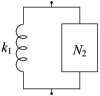
Figure 1: The one-port passive circuit that is the parallel structure of a spring $k_{1}$ and a series-parallel damper-spring-inerter circuit $N_{2}$, where $N_{2}$ contains at most five elements.

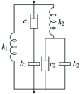
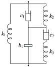
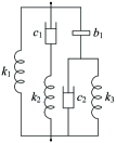
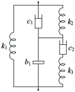
Figure 2: The one-port six-element series-parallel circuit configurations corresponding to Conditions 2–5 of Lemma 4, respectively. All of the configurations belong to the structure in Fig. 1. Here, the element values of the configurations in (a)–(d) are positive and finite.

Table 1: The element values of the configurations in Fig. 2, where $a_{i},d_{j}$ for $i,j=0,1,2$ satisfy (3).

Configuration	Element value expressions
Fig. 2	$c_{1}=\displaystyle\frac{d_{2}}{a_{2}}$, $c_{2}=\displaystyle\frac{d_{0}}{a_{0}}$, $k_{1}=\displaystyle\frac{\alpha_{0}}{\beta_{1}}$, $k_{2}=\displaystyle\frac{d_{0}}{a_{1}}$, $b_{1}=\displaystyle\frac{a_{1}d_{1}-a_{2}d_{0}}{a_{1}a_{0}}$, $b_{2}=\displaystyle\frac{a_{2}d_{0}}{a_{1}a_{0}}$
Fig. 2	$c_{1}=\displaystyle\frac{d_{2}}{a_{2}}$, $c_{2}=\displaystyle\frac{d_{0}}{a_{0}}$, $k_{1}=\displaystyle\frac{\alpha_{0}}{\beta_{1}}$, $k_{2}=\displaystyle\frac{d_{1}d_{0}}{a_{1}d_{1}-a_{0}d_{2}}$, $k_{3}=\displaystyle\frac{d_{1}d_{0}}{a_{0}d_{2}}$, $b_{1}=\displaystyle\frac{d_{1}}{a_{0}}$
Fig. 2	$c_{1}=\displaystyle\frac{d_{0}}{a_{0}}$, $c_{2}=\displaystyle\frac{d_{2}}{a_{2}}$, $k_{1}=\displaystyle\frac{\alpha_{0}}{\beta_{1}}$, $k_{2}=\displaystyle\frac{a_{1}d_{1}-a_{0}d_{2}}{a_{2}a_{1}}$, $k_{3}=\displaystyle\frac{a_{0}d_{2}}{a_{2}a_{1}}$, $b_{1}=\displaystyle\frac{d_{2}}{a_{1}}$
Fig. 2	$c_{1}=\displaystyle\frac{d_{0}}{a_{0}}$, $c_{2}=\displaystyle\frac{d_{2}}{a_{2}}$, $k_{1}=\displaystyle\frac{\alpha_{0}}{\beta_{1}}$, $k_{2}=\displaystyle\frac{d_{1}}{a_{2}}$, $b_{1}=\displaystyle\frac{d_{2}d_{1}}{a_{1}d_{1}-a_{2}d_{0}}$, $b_{2}=\displaystyle\frac{d_{2}d_{1}}{a_{2}d_{0}}$

The above lemma shows the realization results by completely removing the pole at $s=0$, and the following lemma further presents the possible configurations generated by the partial removal of such a pole in order to provide the spring $k_{1}$ in Fig. 1.

Lemma 5

For any admittance $Y(s)$ in (1) that satisfies Assumption 1 and does not satisfy the conditions of Lemma 4, $Y(s)$ is realizable by a one-port series-parallel damper-spring-inerter circuit containing at most six elements as in Fig. 1, if and only if $Y(s)$ can be realized by one of the circuit configurations in Fig. 3.

Proof: The details of this proof can be referred to Appendix B. In the proof, Lemmas 2 and 3 are utilized to establish the realization constraints of $N_{2}$ as in Fig. 1, which are further applied to derive the configurations in Fig. 3. $\blacksquare$

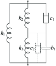
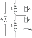
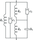
Figure 3: The one-port series-parallel circuit configurations containing at most six elements, which can realize the admittance $Y(s)$ in (1) that satisfies Assumption 1 and does not satisfy the conditions of Lemma 4. Here, the element value of the damper $c_{2}$ in (a) satisfies $c_{2}\geq 0$ (this damper is open-circuited when $c_{2}=0$), and all the other element values in (a)–(c) are positive and finite.

Then, the following Lemmas 6–8 present the realizability conditions and element value expressions of the configurations in Fig. 3.

Lemma 6

Any admittance $Y(s)$ in (1) satisfying Assumption 1 can be realized by the circuit configuration in Fig. 3 ($c_{2}$ can be zero), if and only if there exits a positive root $x>0$ for the equation

$$\begin{split}\Delta_{\beta}x^{2}+2(\beta_{2}\beta_{3}\mathcal{B}_{23}-(\beta_{2}^{2}-2\beta_{1}\beta_{3})\mathcal{B}_{33}-2\beta_{3}^{2}\mathcal{B}_{13})x+(\beta_{2}\mathcal{B}_{33}-\beta_{3}\mathcal{B}_{23})^{2}=0,\end{split}$$ (4a)

such that

$$0<x\leq\tilde{\mathcal{B}}_{23},$$ (4b)

$$\beta_{2}\mathcal{B}_{33}-\beta_{3}\mathcal{B}_{23}<\beta_{2}x<\beta_{2}\mathcal{B}_{33}+\beta_{3}\mathcal{M}_{23},$$ (4c)

and

$$2x^{2}-(\tilde{\mathcal{B}}_{23}+2\mathcal{B}_{33})x+\alpha_{3}(\beta_{2}\mathcal{B}_{33}-\beta_{3}\mathcal{B}_{23})>0.$$ (4d)

Moreover, the element values can be expressed as

$$\begin{split}c_{1}=\frac{\alpha_{3}}{\beta_{3}},~{}~{}c_{2}=\frac{\alpha_{3}(\tilde{\mathcal{B}}_{23}-x)}{\beta_{3}x},~{}~{}k_{1}=\frac{2x^{2}-(\tilde{\mathcal{B}}_{23}+2\mathcal{B}_{33})x+\alpha_{3}(\beta_{2}\mathcal{B}_{33}-\beta_{3}\mathcal{B}_{23})}{2\beta_{3}^{2}x},\\ k_{2}=\frac{\alpha_{3}(\beta_{2}x-(\beta_{2}\mathcal{B}_{33}-\beta_{3}\mathcal{B}_{23}))}{2\beta_{3}^{2}x},~{}~{}k_{3}=\frac{\alpha_{3}(-\beta_{2}x+(\beta_{2}\mathcal{B}_{33}+\beta_{3}\mathcal{M}_{23}))}{2\beta_{3}^{2}x},~{}~{}b_{1}=\frac{\alpha_{3}^{2}}{x}.\end{split}$$ (5)

Proof: The details of the proof are presented in Appendix C. $\blacksquare$

Lemma 7

Any admittance $Y(s)$ in (1) satisfying Assumption 1 can be realized by the circuit configuration in Fig. 3, if and only if there exists positive roots $x>0$ and $y>0$ for the equations

$$\begin{split}\tilde{\mathcal{B}}_{11}\tilde{\mathcal{B}}_{12}y^{2}+(\alpha_{0}-\beta_{1}x)\big{(}(\beta_{3}\tilde{\mathcal{B}}_{11}+\beta_{1}\tilde{\mathcal{B}}_{13})x-(\alpha_{2}\tilde{\mathcal{B}}_{11}+\alpha_{0}\tilde{\mathcal{B}}_{13})\big{)}y+2\alpha_{3}(\alpha_{0}-\beta_{1}x)^{3}=0\end{split}$$ (6a)

and

$$\begin{split}\beta_{1}\tilde{\mathcal{B}}_{11}^{3}y^{4}+\tilde{\mathcal{B}}_{11}^{2}&(\alpha_{0}-\beta_{1}x)(\beta_{1}\beta_{2}x+\mathcal{B}_{12}-2\tilde{\mathcal{B}}_{11})y^{3}\\ &+\tilde{\mathcal{B}}_{11}(\alpha_{0}-\beta_{1}x)^{2}\big{(}\tilde{\mathcal{B}}_{11}(\alpha_{1}-\beta_{2}x)+\beta_{3}(\alpha_{0}-\beta_{1}x)^{2}\big{)}y^{2}-\alpha_{3}(\alpha_{0}-\beta_{1}x)^{6}=0,\end{split}$$ (6b)

such that

$$\alpha_{0}-\beta_{1}y<\beta_{1}x<\alpha_{0}$$ (6c)

and

$$\beta_{3}\tilde{\mathcal{B}}_{11}y^{2}-\alpha_{3}(\alpha_{0}-\beta_{1}x)^{2}>0.$$ (6d)

Moreover, the element values can be expressed as

$$\begin{split}c_{1}=\frac{\tilde{\mathcal{B}}_{11}y^{2}}{(\alpha_{0}-\beta_{1}x)^{2}},~{}~{}c_{2}=\frac{\alpha_{3}\tilde{\mathcal{B}}_{11}y^{2}}{\beta_{3}\tilde{\mathcal{B}}_{11}y^{2}-\alpha_{3}(\alpha_{0}-\beta_{1}x)^{2}},~{}~{}k_{1}=x,\\ k_{2}=y,~{}~{}k_{3}=\frac{y(\alpha_{0}-\beta_{1}x)}{\beta_{1}(x+y)-\alpha_{0}},~{}~{}b_{1}=\frac{\alpha_{3}(\alpha_{0}-\beta_{1}x)^{2}}{\tilde{\mathcal{B}}_{11}(\beta_{1}(x+y)-\alpha_{0})}.\end{split}$$ (7)

Proof: The derivation process is similar to that of Lemma 6, and the details of the proof are presented in the supplementary material [58, Section II.1]. $\blacksquare$

Lemma 8

Any admittance $Y(s)$ in (1) satisfying Assumption 1 can be realized by the circuit configuration in Fig. 3, if and only if there exits a positive root $x>0$ for the equation

$$\begin{split}\Delta_{\beta}x^{2}-4\beta_{3}(2\beta_{1}\mathcal{B}_{23}-\beta_{2}(\mathcal{B}_{22}-2\mathcal{B}_{13}))x-4\beta_{3}(\beta_{1}\mathcal{B}_{23}^{2}-\beta_{2}\mathcal{B}_{23}(\mathcal{B}_{22}-2\mathcal{B}_{13})+\beta_{2}\mathcal{B}_{12}\mathcal{B}_{33})=0,\end{split}$$ (8a)

such that

$$\max\left\{-2\mathcal{B}_{23},-\frac{\beta_{3}\mathcal{B}_{23}+\beta_{2}\mathcal{B}_{33}}{\beta_{3}}\right\}<x<\alpha_{2}\beta_{2}-\mathcal{B}_{23}$$ (8b)

and

$$(\beta_{2}^{2}-2\beta_{1}\beta_{3})x-2\beta_{3}(\beta_{1}\mathcal{B}_{23}-\beta_{2}(\mathcal{B}_{22}-\mathcal{B}_{13}))<0.$$ (8c)

Moreover, the element values can be expressed as

$$\begin{split}c_{1}=\frac{\alpha_{2}\beta_{2}-\mathcal{B}_{23}-x}{\beta_{2}^{2}},~{}~{}c_{2}=\frac{\beta_{3}x+\beta_{3}\mathcal{B}_{23}+\beta_{2}\mathcal{B}_{33}}{\beta_{2}^{2}\beta_{3}},~{}~{}b_{1}=\frac{\beta_{3}x+\beta_{3}\mathcal{B}_{23}+\beta_{2}\mathcal{B}_{33}}{\beta_{2}^{3}},\\ k_{1}=\frac{x}{2\beta_{2}\beta_{3}},~{}~{}k_{2}=\frac{x+2\mathcal{B}_{23}}{2\beta_{2}\beta_{3}},~{}~{}k_{3}=\frac{-(\beta_{2}^{2}-2\beta_{1}\beta_{3})x+2\beta_{3}(\beta_{1}\mathcal{B}_{23}-\beta_{2}(\mathcal{B}_{22}-\mathcal{B}_{13}))}{2\beta_{2}^{3}\beta_{3}}.\end{split}$$ (9)

Proof: The derivation process is similar to that of Lemma 6, and the details of the proof are presented in the supplementary material [58, Section II.2]. $\blacksquare$

Combining Lemmas 4–8 can yield the main theorem of this subsection as follows.

Theorem 1

Any admittance $Y(s)$ in (1) satisfying Assumption 1 is realizable by a one-port series-parallel damper-spring-inerter circuit containing at most six elements as in Fig. 1, if and only if $Y(s)$ satisfies one of the conditions in Lemmas 4 and 6–8. Moreover, if Condition 1 in Lemma 4 holds, then the Foster preamble can be utilized to realize $Y(s)$ as the required circuit; if one of Conditions 2–5 in Lemma 4 or one of the conditions in Lemmas 6–8 holds, then $Y(s)$ can be realized by one of the circuit configurations in Figs. 2 and 3.

Proof: Suppose that the conditions in Lemma 4 do not hold. Then, it follows from Lemma 5 that the circuit configurations that can realize all the other possible admittances $Y(s)$ in this theorem are shown in Fig. 3. By Lemmas 6–8, one can finally prove this theorem. $\blacksquare$

4.3 Realization as Other Series-Parallel Structures

This subsection will further investigate the cases when the realization circuits do not belong to the structure in Fig. 1, which means that the conditions of Theorem 1 do not hold. The main result of this subsection is shown in Theorem 2, where the necessary and sufficient condition for the realizability is the union of the conditions in Lemmas 10–21, and the admittance can be realized by one of the circuit configurations in Figs. 4 and 5.

Lemma 9

For any admittance $Y(s)$ in (1) that satisfies Assumption 1 and does not satisfies the conditions of Theorem 1, $Y(s)$ is realizable by a one-port series-parallel damper-spring-inerter circuit containing no more than six elements, if and only if $Y(s)$ can be realized by one of the circuit configurations in Figs. 4 and 5.

Proof: The details of the proof can be referred to Appendix D. In the proof, a series of realization constraints on the types of elements and constraints on the structures are presented by Lemmas 2 and 3 when the conditions of Theorem 1 do not hold, which are further applied to derive the configurations in Figs. 4 and 5. $\blacksquare$

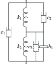
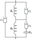
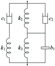
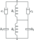
Figure 4: The one-port series-parallel circuit configurations containing at most six elements, which can realize the admittance $Y(s)$ in (1) that satisfies Assumption 1 and does not satisfy the conditions of Theorem 1. Here, the element value of the damper $c_{3}$ in (a) satisfies $c_{3}\geq 0$ (this damper is open-circuited when $c_{3}=0$), and all the other element values in (a)–(d) are positive and finite.

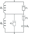
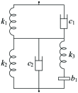
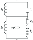
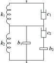
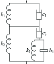
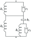
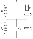
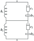
Figure 5: The one-port series-parallel circuit configurations containing at most six elements, which can realize the admittance $Y(s)$ in (1) that satisfies Assumption 1 and does not satisfy the conditions of Theorem 1. Here, the element values of the dampers $c_{2}$ and $c_{3}$ in (a) satisfy $c_{2}^{-1}\geq 0$ and $c_{3}\geq 0$, where the damper $c_{2}$ is short-circuited when $c_{2}^{-1}=0$, the damper $c_{3}$ is open-circuited when $c_{3}=0$, and $c_{2}^{-1}=0$ and $c_{3}=0$ cannot simultaneously hold; all the other element values in (a)–(h) are positive and finite.

Then, the following Lemmas 10–21 present the realizability conditions and element value expressions of the circuit configurations in Figs. 4 and 5.

Lemma 10

Any admittance $Y(s)$ in (1) satisfying Assumption 1 is realizable by the circuit configuration in Fig. 4 ($c_{3}$ can be zero), if and only if there exits a positive root $x>0$ for the equation

$$\begin{split}\beta_{3}^{2}\Delta_{\beta}x^{2}-2\beta_{3}(\beta_{2}\mathcal{M}_{23}-2\beta_{3}(\alpha_{2}\beta_{1}+\alpha_{0}\beta_{3}))x+(\mathcal{B}_{23}^{2}-4\mathcal{B}_{13}\mathcal{B}_{33})=0,\end{split}$$ (10a)

such that

$$x\geq\frac{\mathcal{B}_{23}}{\beta_{2}\beta_{3}},$$ (10b)

$$x>\max\left\{\frac{\alpha_{0}}{\beta_{1}},-\frac{\mathcal{B}_{23}}{\beta_{2}\beta_{3}}\right\},$$ (10c)

and

$$\beta_{2}\beta_{3}x^{2}-\mathcal{M}_{23}x+2\alpha_{0}\alpha_{3}\leq 0.$$ (10d)

Moreover, the element values can be expressed as

$$\begin{split}c_{1}=\frac{\beta_{2}\beta_{3}x^{2}-\mathcal{M}_{23}x+2\alpha_{0}\alpha_{3}}{-2\beta_{3}(\beta_{1}x-\alpha_{0})},~{}~{}c_{2}=\frac{x(\beta_{2}\beta_{3}x+\mathcal{B}_{23})}{2\beta_{3}(\beta_{1}x-\alpha_{0})},\\ c_{3}=\frac{x(\beta_{2}\beta_{3}x-\mathcal{B}_{23})}{2\beta_{3}(\beta_{1}x-\alpha_{0})},~{}~{}k_{1}=x,~{}~{}k_{2}=\frac{\alpha_{0}x}{\beta_{1}x-\alpha_{0}},~{}~{}b_{1}=\frac{\beta_{3}x^{2}}{\beta_{1}x-\alpha_{0}}.\end{split}$$ (11)

Proof: The derivation process is similar to that of Lemma 6, and the details of the proof are presented in the supplementary material [58, Section III.1]. $\blacksquare$

Lemma 11

Any admittance $Y(s)$ in (1) satisfying Assumption 1 is realizable by the circuit configuration in Fig. 4, if and only if there exits positive roots $x>0$ and $y>0$ for the two equations

$$\begin{split}\beta_{1}(\beta_{1}x-2\alpha_{0})(\beta_{1}x-\alpha_{0})y^{2}-\beta_{2}x(\beta_{1}x-\alpha_{0})^{2}y+x^{3}(\beta_{1}^{2}\beta_{3}x+\beta_{2}\tilde{\mathcal{B}}_{11}-\alpha_{2}\beta_{1}^{2})=0\end{split}$$ (12a)

and

$$\begin{split}\beta_{1}(\beta_{1}x-\alpha_{0})^{2}y^{3}-\beta_{1}\beta_{2}x^{2}(\beta_{1}x-\alpha_{0})y^{2}+\beta_{3}x^{2}(\beta_{1}x+\alpha_{0})(\beta_{1}x-\alpha_{0})y-x^{4}(\beta_{1}\mathcal{B}_{23}-\beta_{2}\mathcal{B}_{13})=0,\end{split}$$ (12b)

such that

$$0<(\beta_{1}x-\alpha_{0})y<\beta_{2}x^{2}$$ (12c)

and

$$\begin{split}0<(\beta_{1}x-\alpha_{0})^{2}y^{2}-&\beta_{2}x^{2}(\beta_{1}x-\alpha_{0})y+\beta_{1}\beta_{3}x^{4}<\frac{\alpha_{3}\beta_{1}x^{4}}{y}.\end{split}$$ (12d)

Moreover, the element values can be expressed as

$$\begin{split}c_{1}=\frac{\alpha_{3}\beta_{1}x^{4}-y((\beta_{1}x-\alpha_{0})^{2}y^{2}-\beta_{2}x^{2}(\beta_{1}x-\alpha_{0})y+\beta_{1}\beta_{3}x^{4})}{\beta_{1}\beta_{3}x^{4}},\\ c_{2}=y,~{}~{}c_{3}=\frac{(\beta_{1}x-\alpha_{0})^{2}y^{2}-\beta_{2}x^{2}(\beta_{1}x-\alpha_{0})y+\beta_{1}\beta_{3}x^{4}}{(\beta_{1}x-\alpha_{0})(\beta_{2}x^{2}-(\beta_{1}x-\alpha_{0})y)},\\ k_{1}=x,~{}~{}k_{2}=\frac{\alpha_{0}x}{\beta_{1}x-\alpha_{0}},~{}~{}b_{1}=\frac{(\beta_{1}x-\alpha_{0})^{2}y^{2}-\beta_{2}x^{2}(\beta_{1}x-\alpha_{0})y+\beta_{1}\beta_{3}x^{4}}{\beta_{1}x^{2}(\beta_{1}x-\alpha_{0})}.\end{split}$$ (13)

Proof: The derivation process is similar to that of Lemma 6, and the details of the proof are presented in the supplementary material [58, Section III.2]. $\blacksquare$

Lemma 12

Any admittance $Y(s)$ in (1) satisfying Assumption 1 is realizable by the circuit configuration in Fig. 4, if and only if

$$\beta_{1}\tilde{\mathcal{B}}_{13}+4\beta_{3}\mathcal{B}_{12}\geq 0,$$ (14a)

and there exits a positive root $$x>0$$ for the equation

$$\begin{split}(2\beta_{2}^{2}+\beta_{1}\beta_{3})x^{2}-\beta_{2}(3\beta_{2}\mathcal{B}_{23}+\alpha_{2}(\beta_{2}^{2}+2\beta_{1}\beta_{3}))x+\beta_{2}^{2}(\mathcal{B}_{23}^{2}+\alpha_{2}\beta_{2}\mathcal{B}_{23}+\alpha_{2}^{2}\beta_{1}\beta_{3})=0,\end{split}$$ (14b)

such that

$$\mathcal{B}_{23}<x<\min\{\tilde{\mathcal{B}}_{13},\alpha_{2}\beta_{2}\}$$ (14c)

and

$$x=\frac{1}{2}\left(\tilde{\mathcal{B}}_{13}\pm\sqrt{\tilde{\mathcal{B}}_{13}^{2}+4\mathcal{B}_{12}\tilde{\mathcal{B}}_{33}}\right).$$ (14d)

Moreover, the element values can be expressed as

$$\begin{split}c_{1}=\frac{x-\mathcal{B}_{23}}{\beta_{1}\beta_{3}},~{}~{}c_{2}=\frac{b_{1}k_{1}^{2}+c_{1}^{2}k_{2}+c_{1}^{2}k_{3}}{c_{1}k_{1}},\\ k_{1}=\frac{\alpha_{2}\beta_{2}-x}{\beta_{2}\beta_{3}},~{}~{}k_{2}=\frac{x}{\beta_{2}\beta_{3}},~{}~{}k_{3}=\frac{\tilde{\mathcal{B}}_{13}-x}{\beta_{2}\beta_{3}},~{}~{}b_{1}=\frac{\alpha_{3}}{\beta_{2}}.\end{split}$$ (15)

Proof: The details of the proof are presented in Appendix E. $\blacksquare$

Lemma 13

Any admittance $Y(s)$ in (1) satisfying Assumption 1 is realizable by the circuit configuration in Fig. 4, if and only if

$$\Delta_{y}\geq 0,$$ (16a)

$$\alpha_{2}\tilde{\mathcal{B}}_{11}+\alpha_{1}\mathcal{B}_{13}>0,$$ (16b)

and there exits a positive root $$x>0$$ for the equation

$$\begin{split}\beta_{3}\tilde{\mathcal{B}}_{11}&(\alpha_{2}\beta_{2}+\alpha_{1}\beta_{3})x^{2}-\tilde{\mathcal{B}}_{23}\tilde{\mathcal{B}}_{11}(\alpha_{2}\tilde{\mathcal{B}}_{11}+\alpha_{1}\mathcal{B}_{13})x+\alpha_{1}^{2}\beta_{3}(\alpha_{2}\tilde{\mathcal{B}}_{11}+\alpha_{1}\mathcal{B}_{13})^{2}=0,\end{split}$$ (16c)

such that

$$x=\frac{\alpha_{2}\tilde{\mathcal{B}}_{11}+\alpha_{1}\mathcal{B}_{13}}{2\beta_{1}\beta_{3}}\cdot\left(\beta_{2}\pm\sqrt{\Delta_{y}}\right).$$ (16d)

Moreover, the element values can be expressed as

$$\begin{split}c_{1}=\frac{x}{\tilde{\mathcal{B}}_{11}},~{}~{}c_{2}=\frac{b_{1}^{2}k_{1}+b_{1}^{2}k_{2}+b_{2}c_{1}^{2}}{b_{1}c_{1}},~{}~{}k_{1}=\frac{\alpha_{0}\alpha_{1}}{\tilde{\mathcal{B}}_{11}},\\ k_{2}=\frac{\alpha_{1}}{\beta_{2}},~{}~{}b_{1}=\frac{\alpha_{2}\tilde{\mathcal{B}}_{11}+\alpha_{1}\mathcal{B}_{13}}{\beta_{1}\tilde{\mathcal{B}}_{11}},~{}~{}b_{2}=\frac{\alpha_{1}^{2}\beta_{3}}{\beta_{2}\tilde{\mathcal{B}}_{11}}.\end{split}$$ (17)

Proof: The derivation process is similar to that of Lemma 12, and the details of the proof are presented in the supplementary material [58, Section III.3]. $\blacksquare$

Lemma 14

Any admittance $Y(s)$ in (1) satisfying Assumption 1 is realizable by the circuit configuration in Fig. 5 ($c_{2}$ or $c_{3}$ can be infinite), if and only if at least one of the following two conditions holds:

1. there exists a negative root $y<0$ for the equation

   $$\alpha_{3}y^{3}+\alpha_{2}y^{2}+\alpha_{1}y+\alpha_{0}=0,$$ (18)

   such that $\Gamma_{1}:=\beta_{3}y^{2}+\beta_{2}y+\beta_{1}$, $\Gamma_{2}:=-2\alpha_{3}y^{3}-\alpha_{2}y^{2}+\alpha_{0}$, $\Gamma_{3}:=2\tilde{\mathcal{B}}_{13}y^{2}+\tilde{\mathcal{M}}_{12}y-\mathcal{B}_{12}$, $\Gamma_{4}:=-\tilde{\mathcal{B}}_{33}y^{3}+\mathcal{B}_{33}y^{2}+\tilde{\mathcal{B}}_{13}y-\mathcal{B}_{12}$, and $\Gamma_{5}:=\beta_{1}\beta_{3}y^{2}(\alpha_{3}y+\alpha_{2})^{2}+(\tilde{\mathcal{B}}_{13}y-\mathcal{B}_{13})^{2}-\beta_{2}y(\alpha_{3}y+\alpha_{2})(\tilde{\mathcal{B}}_{13}y+\mathcal{B}_{13})+\mathcal{B}_{12}\tilde{\mathcal{B}}_{23}y$, and $\Gamma_{6}:=-y(2\alpha_{3}y+\alpha_{2})(\tilde{\mathcal{B}}_{13}y^{2}+\alpha_{2}\beta_{1}y-\mathcal{B}_{12})-\alpha_{0}(\tilde{\mathcal{B}}_{13}y-\mathcal{B}_{13})$ have the same sign, where $\Gamma_{k}$ is nonzero for $k=1,2,...,5$ and $\Gamma_{6}$ can be zero;

2. $\mathcal{M}_{23}^{2}+8\mathcal{B}_{13}\tilde{\mathcal{B}}_{23}\geq 0$, and there exists a positive root $x>0$ for the equation

   $$\beta_{3}^{3}x^{3}-\alpha_{2}\beta_{3}^{2}x^{2}+\alpha_{1}\tilde{\mathcal{B}}_{33}x-\alpha_{0}\alpha_{3}^{2}=0,$$ (19a)

   such that

   $$x>\max\left\{\frac{\alpha_{0}}{\beta_{1}},\frac{\alpha_{0}\alpha_{3}}{\alpha_{1}\beta_{3}}\right\}$$ (19b)

   and

   $$x=\frac{\mathcal{M}_{23}\pm\sqrt{\mathcal{M}_{23}^{2}+8\mathcal{B}_{13}\tilde{\mathcal{B}}_{23}}}{2\beta_{2}\beta_{3}}.$$ (19c)

Moreover, if Condition 1 holds, then the element values can be expressed as

$$\begin{split}c_{1}=-\frac{\Gamma_{2}}{y\Gamma_{1}},~{}~{}c_{2}=-\frac{\Gamma_{2}^{2}\Gamma_{5}}{y\Gamma_{3}^{2}\Gamma_{4}},~{}~{}c_{3}=-\frac{\Gamma_{2}\Gamma_{6}}{y\Gamma_{3}^{2}},~{}~{}k_{1}=\frac{\Gamma_{2}}{\Gamma_{1}},~{}~{}k_{2}=-\frac{\alpha_{0}\Gamma_{2}}{y\Gamma_{3}},~{}~{}b_{1}=-\frac{\Gamma_{2}^{2}\Gamma_{5}}{y\Gamma_{3}^{3}};\end{split}$$ (20)

if Condition 2 holds, then the element values can be expressed as

$$\begin{split}c_{1}=\frac{\alpha_{3}}{\beta_{3}},~{}~{}c_{2}=\infty,~{}~{}c_{3}=\frac{\alpha_{1}\beta_{3}x-\alpha_{0}\alpha_{3}}{\beta_{3}(\beta_{1}x-\alpha_{0})},~{}~{}k_{1}=x,~{}~{}k_{2}=\frac{\alpha_{0}x}{\beta_{1}x-\alpha_{0}},~{}~{}b_{1}=\frac{\beta_{3}x^{2}}{\beta_{1}x-\alpha_{0}}.\end{split}$$ (21)

Proof: The derivation process is similar to that of Lemma 6, and the details of the proof are presented in the supplementary material [58, Section IV.1]. $\blacksquare$

Lemma 15

Any admittance $Y(s)$ in (1) satisfying Assumption 1 is realizable by the circuit configuration in Fig. 5, if and only if

$$\Delta_{\alpha}>0,$$ (22a)

$$\mathcal{B}_{23}<\min\left\{\frac{\alpha_{3}\mathcal{B}_{12}}{\alpha_{1}},\frac{\beta_{3}\mathcal{B}_{12}}{\beta_{1}}\right\},$$ (22b)

and

$$\mathcal{B}_{23}^{3}+\alpha_{2}\beta_{2}\mathcal{B}_{23}^{2}+\alpha_{1}\beta_{2}\tilde{\mathcal{B}}_{23}\mathcal{B}_{23}-\tilde{\mathcal{B}}_{23}^{2}\mathcal{B}_{12}=0.$$ (22c)

Moreover, the element values can be expressed as

$$\begin{split}c_{1}=\frac{-\alpha_{3}(\alpha_{1}\mathcal{B}_{23}-\alpha_{3}\mathcal{B}_{12})}{\mathcal{B}_{23}^{2}},~{}~{}c_{2}=\frac{c_{1}(b_{1}k_{1}^{2}k_{2}+b_{1}k_{1}^{2}k_{3}+c_{1}^{2}k_{2}k_{3})}{k_{1}(b_{1}k_{1}^{2}+c_{1}^{2}k_{3})},~{}~{}k_{1}=\frac{\alpha_{1}\mathcal{B}_{23}-\alpha_{3}\mathcal{B}_{12}}{\beta_{2}\mathcal{B}_{23}},\\ k_{2}=\frac{\alpha_{0}(\alpha_{1}\mathcal{B}_{23}-\alpha_{3}\mathcal{B}_{12})}{\alpha_{1}(\beta_{1}\mathcal{B}_{23}-\beta_{3}\mathcal{B}_{12})},~{}~{}k_{3}=\frac{\Delta_{\alpha}(\alpha_{1}\mathcal{B}_{23}-\alpha_{3}\mathcal{B}_{12})}{\alpha_{1}\alpha_{3}(\beta_{1}\mathcal{B}_{23}-\beta_{3}\mathcal{B}_{12})},~{}~{}b_{1}=\frac{\Delta_{\alpha}(\alpha_{1}\mathcal{B}_{23}-\alpha_{3}\mathcal{B}_{12})}{\alpha_{1}^{2}(\beta_{1}\mathcal{B}_{23}-\beta_{3}\mathcal{B}_{12})}.\end{split}$$ (23)

Proof: The derivation process is similar to that of Lemma 12, and the details of the proof are presented in the supplementary material [58, Section IV.2]. $\blacksquare$

Lemma 16

Any admittance $Y(s)$ in (1) satisfying Assumption 1 is realizable by the circuit configuration in Fig. 5, if and only if

$$\Delta_{\alpha}>0,$$ (24a)

and there exists a positive root $$x>0$$ for the equation

$$\begin{split}\beta_{3}^{2}(\alpha_{3}\tilde{\mathcal{B}}_{12}-\alpha_{2}^{2}\beta_{2})x^{2}+\alpha_{2}\beta_{3}^{2}\Delta_{\alpha}x+\alpha_{0}\alpha_{3}^{2}(\mathcal{B}_{23}-\alpha_{2}\beta_{2})=0,\end{split}$$ (24b)

such that

$$x>\frac{\alpha_{0}}{\beta_{1}}$$ (24c)

and

$$\beta_{3}^{3}x^{3}-\alpha_{2}\beta_{3}^{2}x^{2}+\alpha_{1}\tilde{\mathcal{B}}_{33}x-\alpha_{0}\alpha_{3}^{2}=0.$$ (24d)

Moreover, the element values can be expressed as

$$\begin{split}c_{1}=\frac{\alpha_{3}}{\beta_{3}},~{}~{}c_{2}=\frac{c_{1}k_{3}(b_{1}k_{1}^{2}+c_{1}^{2}k_{2})}{k_{1}(b_{1}k_{1}^{2}+c_{1}^{2}k_{2}+c_{1}^{2}k_{3})},~{}~{}k_{1}=x,\\ k_{2}=\frac{\alpha_{0}x}{\beta_{1}x-\alpha_{0}},~{}~{}k_{3}=\frac{\Delta_{\alpha}x}{\alpha_{3}(\beta_{1}x-\alpha_{0})},~{}~{}b_{1}=\frac{\alpha_{2}x}{\beta_{1}x-\alpha_{0}}.\end{split}$$ (25)

Proof: The derivation process is similar to that of Lemma 12, and the details of the proof are presented in the supplementary material [58, Section IV.3]. $\blacksquare$

Lemma 17

Any admittance $Y(s)$ in (1) satisfying Assumption 1 is realizable by the circuit configuration in Fig. 5, if and only if

$$\Delta_{\alpha}>0,$$ (26a)

and there exists a positive root $$x>0$$ for the equation

$$\begin{split}\beta_{3}^{2}(\alpha_{2}\tilde{\mathcal{B}}_{11}+\alpha_{1}\mathcal{B}_{13})x^{2}-\beta_{3}\mathcal{B}_{13}\Delta_{\alpha}x+\alpha_{0}\alpha_{3}(\alpha_{1}\mathcal{B}_{23}+\alpha_{3}\mathcal{B}_{12})=0,\end{split}$$ (26b)

such that

$$x>\frac{\alpha_{0}}{\beta_{1}}$$ (26c)

and

$$\beta_{3}^{3}x^{3}-\alpha_{2}\beta_{3}^{2}x^{2}+\alpha_{1}\tilde{\mathcal{B}}_{33}x-\alpha_{0}\alpha_{3}^{2}=0.$$ (26d)

Moreover, the element values can be expressed as

$$\begin{split}c_{1}=\frac{\alpha_{3}}{\beta_{3}},~{}~{}c_{2}=\frac{b_{2}k_{1}(b_{1}k_{1}^{2}+c_{1}^{2}k_{2})}{c_{1}(b_{1}k_{1}^{2}+b_{2}k_{1}^{2}+c_{1}^{2}k_{2})},~{}~{}k_{1}=x,\\ k_{2}=\frac{\alpha_{0}x}{\beta_{1}x-\alpha_{0}},~{}~{}b_{1}=\frac{\alpha_{0}\alpha_{3}x}{\alpha_{1}(\beta_{1}x-\alpha_{0})},~{}~{}b_{2}=\frac{\Delta_{\alpha}x}{\alpha_{1}(\beta_{1}x-\alpha_{0})}.\end{split}$$ (27)

Proof: The derivation process is similar to that of Lemma 12, and the details of the proof are presented in the supplementary material [58, Section IV.4]. $\blacksquare$

Lemma 18

Any admittance $Y(s)$ in (1) satisfying Assumption 1 is realizable by the circuit configuration in Fig. 5, if and only if

$$\tilde{\mathcal{B}}_{12}>0,$$ (28a)

$$\beta_{2}(\beta_{1}\Delta_{\alpha}+\alpha_{2}\mathcal{B}_{12})-\tilde{\mathcal{B}}_{12}^{2}>0,$$ (28b)

and

$$\begin{split}(\mathcal{B}_{23}+\alpha_{2}\beta_{2})(\beta_{1}\Delta_{\alpha}+\alpha_{2}\mathcal{B}_{12})^{2}-\alpha_{2}\tilde{\mathcal{B}}_{12}^{2}(\beta_{1}\Delta_{\alpha}+\alpha_{2}\mathcal{B}_{12})+\alpha_{0}\alpha_{3}\tilde{\mathcal{B}}_{12}^{3}=0.\end{split}$$ (28c)

Moreover, the element values can be expressed as

$$\begin{split}c_{1}=\frac{\Delta_{\alpha}(\beta_{1}\Delta_{\alpha}+\alpha_{2}\mathcal{B}_{12})^{2}}{\tilde{\mathcal{B}}_{12}(\alpha_{0}\alpha_{2}\tilde{\mathcal{B}}_{12}^{2}+(\beta_{1}\Delta_{\alpha}+\alpha_{2}\mathcal{B}_{12})^{2})},~{}~{}c_{2}=\frac{c_{1}k_{2}(b_{1}k_{1}^{2}+c_{1}^{2}k_{3})}{k_{1}(b_{1}k_{1}^{2}+c_{1}^{2}k_{2}+c_{1}^{2}k_{3})},\\ k_{1}=\frac{\alpha_{0}\Delta_{\alpha}(\beta_{1}\Delta_{\alpha}+\alpha_{2}\mathcal{B}_{12})}{\alpha_{0}\alpha_{2}\tilde{\mathcal{B}}_{12}^{2}+(\beta_{1}\Delta_{\alpha}+\alpha_{2}\mathcal{B}_{12})^{2}},~{}~{}k_{2}=\frac{\Delta_{\alpha}(\beta_{1}\Delta_{\alpha}+\alpha_{2}\mathcal{B}_{12})}{\alpha_{2}(\beta_{2}(\beta_{1}\Delta_{\alpha}+\alpha_{2}\mathcal{B}_{12})-\tilde{\mathcal{B}}_{12}^{2})},\\ k_{3}=\frac{\alpha_{0}\alpha_{3}(\beta_{1}\Delta_{\alpha}+\alpha_{2}\mathcal{B}_{12})}{\alpha_{2}(\beta_{2}(\beta_{1}\Delta_{\alpha}+\alpha_{2}\mathcal{B}_{12})-\tilde{\mathcal{B}}_{12}^{2})},~{}~{}b_{1}=\frac{\alpha_{3}(\beta_{1}\Delta_{\alpha}+\alpha_{2}\mathcal{B}_{12})}{\beta_{2}(\beta_{1}\Delta_{\alpha}+\alpha_{2}\mathcal{B}_{12})-\tilde{\mathcal{B}}_{12}^{2}}.\end{split}$$ (29)

Proof: The derivation process is similar to that of Lemma 12, and the details of the proof are presented in the supplementary material [58, Section IV.5]. $\blacksquare$

Lemma 19

Any admittance $Y(s)$ in (1) satisfying Assumption 1 is realizable by the circuit configuration in Fig. 5, if and only if

$$\Delta_{\alpha}>0,$$ (30a)

$$\tilde{\mathcal{B}}_{11}>0,$$ (30b)

and there exists a positive root $$x>0$$ for the equation

$$\begin{split}\tilde{\mathcal{B}}_{11}(\beta_{1}&\Delta_{\alpha}+\alpha_{1}\mathcal{B}_{13})x^{2}-\alpha_{0}\tilde{\mathcal{B}}_{11}\Delta_{\alpha}x+\alpha_{0}^{3}\alpha_{1}\alpha_{3}=0,\end{split}$$ (30c)

such that

$$\max\left\{\frac{\alpha_{0}}{\beta_{1}},\frac{\alpha_{0}^{2}\alpha_{3}}{\alpha_{2}\tilde{\mathcal{B}}_{11}}\right\}<x<\frac{\alpha_{0}\alpha_{1}}{\tilde{\mathcal{B}}_{11}}$$ (30d)

and

$$\alpha_{3}y^{3}+\alpha_{2}y^{2}+\alpha_{1}y+\alpha_{0}=0,$$ (30e)

where

$$y=-\sqrt{\frac{\alpha_{0}(\tilde{\mathcal{B}}_{11}x-\alpha_{0}\alpha_{1})}{\alpha_{0}^{2}\alpha_{3}-\alpha_{2}\tilde{\mathcal{B}}_{11}x}}.$$ (30f)

Moreover, the element values can be expressed as

$$\begin{split}c_{1}=-\frac{x}{y},~{}~{}c_{2}=\frac{c_{1}(b_{1}k_{1}^{2}k_{2}+b_{1}k_{1}^{2}k_{3}+c_{1}^{2}k_{2}k_{3})}{k_{1}(b_{1}k_{1}^{2}+c_{1}^{2}k_{2})},~{}~{}k_{1}=x,\\ k_{2}=\frac{\alpha_{0}x}{\beta_{1}x-\alpha_{0}},~{}~{}k_{3}=\frac{\alpha_{0}^{2}\alpha_{3}x}{\Delta_{\alpha}(\beta_{1}x-\alpha_{0})},~{}~{}b_{1}=\frac{\alpha_{0}\alpha_{3}x}{\alpha_{1}(\beta_{1}x-\alpha_{0})}.\end{split}$$ (31)

Proof: The derivation process is similar to that of Lemma 12, and the details of the proof are presented in the supplementary material [58, Section IV.6]. $\blacksquare$

Lemma 20

Any admittance $Y(s)$ in (1) satisfying Assumption 1 is realizable by the circuit configuration in Fig. 5, if and only if

$$\tilde{\mathcal{B}}_{11}>0,$$ (32a)

and there are positive roots $$x>0 y>0$$ and for the equations

$$\begin{split}\alpha_{3}(\beta_{1}^{2}\beta_{3}x^{2}+(2\beta_{1}\mathcal{B}_{13}&-\beta_{2}\tilde{\mathcal{B}}_{11})x-\alpha_{0}\mathcal{B}_{13}+\alpha_{1}\tilde{\mathcal{B}}_{11})y\\ &-(\beta_{1}x-\alpha_{0})(\beta_{1}\beta_{3}^{2}x^{2}-\beta_{3}\tilde{\mathcal{M}}_{12}x-\alpha_{2}\mathcal{B}_{13}+\alpha_{3}\tilde{\mathcal{B}}_{11})=0\end{split}$$ (32b)

and

$$\begin{split}(\beta_{2}x-\alpha_{1})\Psi_{2}y^{2}-(\beta_{1}x-\alpha_{0})\Psi_{1}y+\alpha_{0}(\beta_{1}x-\alpha_{0})^{2}\Psi_{0}=0,\end{split}$$ (32c)

such that

$$\beta_{1}x-\alpha_{0}>0,$$ (32d)

$$(\beta_{2}x-\alpha_{1})y+\beta_{1}x-\alpha_{0}>0,$$ (32e)

and

$$\begin{split}(\beta_{2}x-\alpha_{1})\Upsilon_{2}y^{2}+(\beta_{2}x-\alpha_{1})(\beta_{1}x-\alpha_{0})\Upsilon_{1}y+(\beta_{1}x-\alpha_{0})^{2}\Upsilon_{0}=0.\end{split}$$ (32f)

Moreover, the element values can be expressed as

$$\begin{split}c_{1}=\frac{\alpha_{3}}{\beta_{3}},~{}~{}c_{2}=\frac{\tilde{\mathcal{B}}_{11}x^{2}}{(\beta_{1}x-\alpha_{0})^{2}},~{}~{}k_{1}=x,~{}~{}k_{2}=\frac{\alpha_{0}x}{\beta_{1}x-\alpha_{0}},\\ b_{1}=\frac{\alpha_{3}((\beta_{2}x-\alpha_{1})y+\beta_{1}x-\alpha_{0})}{\beta_{3}y(\beta_{1}x-\alpha_{0})},~{}~{}b_{2}=\frac{\beta_{3}x^{2}}{(\beta_{2}x-\alpha_{1})y+\beta_{1}x-\alpha_{0}}.\end{split}$$ (33)

Here, $\Psi_{2}:=\beta_{3}(\alpha_{0}\beta_{2}^{2}-\alpha_{1}\beta_{1}\beta_{2}+\alpha_{2}\beta_{1}^{2})x^{3}-(\alpha_{0}\alpha_{1}\beta_{2}\beta_{3}+2\alpha_{0}\alpha_{2}\beta_{1}\beta_{3}+\alpha_{0}\alpha_{3}\beta_{1}\beta_{2}-\alpha_{1}^{2}\beta_{1}\beta_{3})x^{2}+\alpha_{0}(\alpha_{0}\alpha_{2}\beta_{3}+\alpha_{0}\alpha_{3}\beta_{2}+\alpha_{1}\alpha_{3}\beta_{1})x+\alpha_{0}^{2}\alpha_{1}\alpha_{3}$, $\Psi_{1}:=\beta_{1}^{2}\beta_{3}^{2}x^{4}-\beta_{3}(2\alpha_{0}\beta_{1}\beta_{3}+2\alpha_{0}\beta_{2}^{2}-\alpha_{1}\beta_{1}\beta_{2}+\alpha_{2}\beta_{1}^{2})x^{3}+(\alpha_{0}^{2}\beta_{3}^{2}+3\alpha_{0}\alpha_{1}\beta_{2}\beta_{3}+2\alpha_{0}\alpha_{2}\beta_{1}\beta_{3}+2\alpha_{0}\alpha_{3}\beta_{1}\beta_{2}-\alpha_{1}^{2}\beta_{1}\beta_{3})x^{2}-\alpha_{0}(\alpha_{0}\alpha_{2}\beta_{3}+2\alpha_{0}\alpha_{3}\beta_{2}+\alpha_{1}^{2}\beta_{3}+2\alpha_{1}\alpha_{3}\beta_{1})x+2\alpha_{0}^{2}\alpha_{1}\alpha_{3}$, $\Psi_{0}:=\beta_{2}\beta_{3}x^{2}-\mathcal{M}_{23}x+\alpha_{0}\alpha_{3}$, $\Upsilon_{2}:=\beta_{1}^{2}\beta_{3}^{2}x^{4}+(\alpha_{0}\beta_{2}^{2}\beta_{3}-2\alpha_{0}\beta_{1}\beta_{3}^{2}-\alpha_{1}\beta_{1}\beta_{2}\beta_{3}-\alpha_{3}\beta_{1}^{2}\beta_{2})x^{3}+(\alpha_{0}^{2}\beta_{3}^{2}-\alpha_{0}\alpha_{1}\beta_{2}\beta_{3}+2\alpha_{0}\alpha_{3}\beta_{1}\beta_{2}+\alpha_{1}^{2}\beta_{1}\beta_{3}+\alpha_{1}\alpha_{3}\beta_{1}^{2})x^{2}-\alpha_{0}\alpha_{3}(\alpha_{0}\beta_{2}+2\alpha_{1}\beta_{1})x+\alpha_{0}^{2}\alpha_{1}\alpha_{3}$, $\Upsilon_{1}:=\beta_{1}\beta_{2}\beta_{3}x^{3}-(2\alpha_{1}\beta_{1}\beta_{3}+2\alpha_{3}\beta_{1}^{2}-\alpha_{0}\beta_{2}\beta_{3})x^{2}+4\alpha_{0}\alpha_{3}\beta_{1}x-2\alpha_{0}^{2}\alpha_{3}$, and $\Upsilon_{0}:=\beta_{1}\beta_{2}\beta_{3}x^{3}-\beta_{1}\mathcal{M}_{23}x^{2}+2\alpha_{0}\alpha_{3}\beta_{1}x-\alpha_{0}^{2}\alpha_{3}$.

Proof: The details of the proof are presented in [58, Section IV.7]. $\blacksquare$

Lemma 21

Any admittance $Y(s)$ in (1) satisfying Assumption 1 is realizable by the circuit configuration in Fig. 5, if and only if

$$\tilde{\mathcal{B}}_{11}=0,$$ (34a)

and there are positive roots $$x>0 y>0 z>0$$, , and for the equations

$$\alpha_{0}x\Theta_{0}z^{2}-y\Theta_{1}z+\alpha_{3}^{2}x^{2}y^{2}(\beta_{1}y-\alpha_{0})=0,$$ (34b)

$$\alpha_{0}\Theta_{0}z^{2}+x\Theta_{2}z+\alpha_{0}\alpha_{3}xy^{2}(\beta_{3}x-\alpha_{3})=0,$$ (34c)

and

$$x(\beta_{1}y-\alpha_{0})\Theta_{0}z^{2}-y^{2}\Theta_{3}z+\alpha_{3}^{2}x^{2}y^{2}(\beta_{1}y-\alpha_{0})=0,$$ (34d)

such that

$$\beta_{3}x-\alpha_{3}>0,$$ (34e)

$$\beta_{1}y-\alpha_{0}>0,$$ (34f)

and

$$\Theta_{0}>0.$$ (34g)

Moreover, the element values can be expressed as

$$\begin{split}c_{1}=x,~{}~{}c_{2}=\frac{\alpha_{3}x}{\beta_{3}x-\alpha_{3}},~{}~{}k_{1}=y,~{}~{}k_{2}=\frac{\alpha_{0}y}{\beta_{1}y-\alpha_{0}},~{}~{}b_{1}=z,~{}~{}b_{2}=\frac{\alpha_{3}^{2}xy^{2}}{z\Theta_{0}}.\end{split}$$ (35)

Here, $\Theta_{0}:=-\tilde{\mathcal{B}}_{12}xy+\alpha_{3}y(\beta_{1}y-2\alpha_{0})+\alpha_{0}\alpha_{2}x$, $\Theta_{1}:=\alpha_{0}(\alpha_{2}x-\alpha_{3}y)^{2}-\tilde{\mathcal{B}}_{12}xy(\alpha_{2}x-\alpha_{3}y)+\alpha_{1}\alpha_{3}x^{2}(\beta_{1}y-\alpha_{0})$, $\Theta_{2}:=xy(\beta_{1}\Delta_{\alpha}+\alpha_{1}\mathcal{B}_{13})-\alpha_{0}\Delta_{\alpha}x-\alpha_{1}\alpha_{3}y(\beta_{1}y-2\alpha_{0})$, and $\Theta_{3}:=x^{2}y(\beta_{1}\mathcal{B}_{33}-\beta_{3}\mathcal{B}_{13})-\alpha_{0}\mathcal{B}_{33}x^{2}+2\alpha_{3}\mathcal{B}_{13}xy+\alpha_{3}\tilde{\mathcal{B}}_{13}y^{2}$.

Proof: The details of the proof are presented in [58, Section IV.8]. $\blacksquare$

Theorem 2

For any admittance $Y(s)$ in (1) that satisfies Assumption 1 and does not satisfy the conditions of Theorem 1, $Y(s)$ is realizable by a one-port series-parallel damper-spring-inerter circuit containing at most six elements, if and only if one of the conditions in Lemmas 10–21 holds. Moreover, the realizability conditions correspond to the circuit configurations in Figs. 4 and 5.

Proof: By Lemma 9, the circuit configurations that can realize all the possible cases of $Y(s)$ in this theorem are shown in Figs. 4 and 5. Since the realizability conditions of these circuit configurations are presented in Lemmas 10–21, this theorem can be proved. $\blacksquare$

4.4 Summary

Combining the above discussions, the final result of this paper is summarized.

Theorem 3

Any admittance $Y(s)$ in (1) satisfying Assumption 1 is realizable as a one-port series-parallel damper-spring-inerter circuit containing at most six elements, if and only if $Y(s)$ satisfies one of the conditions in Lemmas 4, 6–8, and 10–21. Moreover, if any of the conditions in Lemma 4 holds, then $Y(s)$ is realizable by the required circuit after extracting the parallel spring $k_{1}=\alpha_{0}/\beta_{1}$ to remove the pole at $s=0$; If one of the conditions in Lemmas 6–8 and 10–21 holds, then $Y(s)$ is realizable by one of the circuit configurations in Figs. 3–5 (summarized in Table 2).

Proof: Any one-port series-parallel damper-spring-inerter circuit realizing $Y(s)$ in this theorem is either the structure in Fig. 1 or any of other possible configurations. Combining Theorems 1 and 2 can imply this theorem. $\blacksquare$

Table 2: The summary of the realization results of the circuit configurations in Figs. 3–5.

Configurations	Realizability results
Fig. 3	Conditions and element value expressions in Lemmas 6–8
Fig. 4	Conditions and element value expressions in Lemmas 10–13
Fig. 5	Conditions and element value expressions in Lemmas 14–21

Remark 1

It is noted that the necessary and sufficient condition in Theorem 3 is the union of the conditions in Lemmas 4, 6–8, and 10–21, which can be described by the set $\mathcal{S}=\{(\alpha_{3},...,\alpha_{0},\beta_{3},...,\beta_{1})~{}|~{}\alpha_{i},\beta_{j}>0\text{ satisfy Assumption~{}\ref{assumption: 01} and the condition in Theorem~{}\ref{theorem: main theorem 03}}\}$. Then, $\mathcal{S}$ is a semi-algebraic subset of the 7-dimensional Euclidean space, whose dimension is equal to the dimension of the positive-real set of $Y(s)$ in Lemma 1. In contrast, the dimension of the realizability set for the five-element realization results in [38] is one less than that of the positive-real set. The five-element series-parallel realization results in [38] can be included by the results of this paper as special cases.

5 Examples of Circuit Synthesis and Passive Controller Optimizations

This section will present several examples to illustrate the circuit synthesis results of this paper, including the passive controller optimizations for a train suspension system. Example 1 is an ideal numerical example, Example 2 presents the mechanical circuit synthesis results for the optimal positive-real admittances in [11], and Example 3 gives the mechanical circuit synthesis results based on the optimization results for the passive controller design of a side-view train suspension system.

Example 1

Consider an admittance $Y(s)$ in (1) with $\alpha_{3}=6$, $\alpha_{2}=13$, $\alpha_{1}=17$, $\alpha_{0}=10$, $\beta_{3}=7$, $\beta_{2}=13$, and $\beta_{1}=15$. Since one can check that none of the conditions in Lemma 4 holds, $Y(s)$ cannot be realized by a one-port six-element series-parallel circuit by completely removing the pole at $s=0$. By the Bott-Duffin circuit synthesis procedure, $Y(s)$ can be realized by a one-port ten-element series-parallel damper-spring-inerter circuit. Then, it is calculated that a negative root of the equation (18) is $y=-1$, such that $\Gamma_{1}=9$, $\Gamma_{2}=9$, $\Gamma_{3}=45$, $\Gamma_{4}=9$, $\Gamma_{5}=1125$, and $\Gamma_{6}=225$ have the same sign. Therefore, Condition 1 of Lemma 14 holds. By the element value expressions in (20), $Y(s)$ can be realized by the one-port six-element series-parallel circuit in Fig. 5 with $c_{1}=1$ Ns/m, $c_{2}=5$ Ns/m, $c_{3}=1$ Ns/m, $k_{1}=1$ N/m, $k_{2}=2$ N/m, and $b_{1}=1$ kg, which saves four elements compared with the circuit realization by the Bott-Duffin procedure.

Example 2

Consider the one-wheel train suspension model in [11, Fig. 1]. By choosing the static stiffness settings of $Q_{1}(s)$ and $Q_{2}(s)$ as $k_{s}=1.41\times 10^{5}$ N/m and $k_{b}=1.26\times 10^{6}$ N/m, it is shown in [11] that the positive-real admittances $Q_{1}(s)$ and $Q_{2}(s)$ in the form of (1) that minimizes the ride comfort index $J_{1}$ can be determined by the BMI optimization method as $Q_{1}(s)=(3212.9s^{3}+2.407\times 10^{5}s^{2}+1.082\times 10^{6}s+7.42\times 10^{6})/(s^{3}+7.674s^{2}+52.627s)$ and $Q_{2}(s)=(13754s^{3}+1.272\times 10^{6}s^{2}+8.294\times 10^{7}s+9.644\times 10^{7})/(s^{3}+65.763s^{2}+76.541s)$. One can verify that $Q_{1}(s)$ satisfies Condition 1 of Lemma 4. By making use of the Foster preamble, $Q_{1}(s)$ is realizable by a one-port six-element series-parallel circuit in Fig. 6 with $c_{1}=0.26455$ Ns/m, $c_{2}=3212.635$ Ns/m, $c_{3}=13465.328$ Ns/m, $k_{1}=k_{s}=1.41\times 10^{5}$ N/m, $k_{2}=80490.163$ N/m, and $b_{1}=1894.339$ kg. It can be checked that $Q_{2}(s)$ does not satisfy any of the conditions in Lemma 4, which means that $Q_{2}(s)$ cannot be realized by any six-element series-parallel circuit by completely removing the pole at $s=0$. It can be checked that $Q_{2}(s)$ satisfies any of the conditions in Lemmas 6–8, which means that the admittance $Q_{2}(s)$ is realizable by one of the one-port six-element series-parallel circuit configurations in Fig. 3. For instance, by the element value expressions in (5) with $x=9.012\times 10^{5}>0$, $Q_{2}(s)$ is realizable as the configuration in Fig. 3 (also shown in Fig. 6) with $c_{1}=13754$ Ns/m, $c_{2}=50.471$ Ns/m, $k_{1}=1.257\times 10^{6}$ N/m, $k_{2}=11828.383$ N/m, $k_{3}=4238.539$ N/m, and $b_{1}=209.912$ kg. In comparison, by utilizing the Bott-Duffin circuit synthesis procedure, $Q_{2}(s)$ is realizable as a ten-element series-parallel circuit as shown in Fig. 6 with $c_{1}=16435.553$ Ns/m, $c_{2}=1047.275$ Ns/m, $c_{3}=84299.893$ Ns/m, $k_{1}=k_{b}=1.26\times 10^{6}$ N/m, $k_{2}=1136.435$ N/m, $k_{3}=4.698\times 10^{5}$ N/m, $k_{4}=3.819\times 10^{6}$ N/m, $c_{1}=16435.553$ Ns/m, $c_{2}=1047.275$ Ns/m, and $c_{3}=84299.893$ Ns/m. Therefore, the results of this paper can save four elements for the physical realization of $Q_{2}(s)$.

Figure 6: (a) The one-port six-element series-parallel circuit realizing the admittance $Q_{1}(s)$ in Example 2; (b) the one-port six-element series-parallel circuit realizing the admittance $Q_{2}(s)$ in Example 2, which is the configuration in Figure 3; (c) the one-port ten-element series-parallel circuit realizing the admittance $Q_{2}(s)$ by making use of the Bott-Duffin circuit synthesis procedure.

The following train suspension control system is a specific case of Appendix A, where the number of positive-real admittances satisfies $m=2$, and the two admittances $Q_{1}(s)=Q_{2}(s)$ as in (1) can be expressed in (A.2) with the McMillan degree being three.

Consider a side-view train suspension model as shown in Fig. 7 (see [12]), where $m_{s}$, $I_{s}$, $z_{s}$, and $\theta_{s}$ denote the mass, pitch inertia, vertical displacement, and pitch angle of train body; $m_{b1}$, $I_{b1}$, $z_{s1}$, and $\theta_{b1}$ denote the mass, pitch inertia, vertical displacement, and pitch angle of the front bogie; $m_{b2}$, $I_{b2}$, $z_{s2}$, and $\theta_{b2}$ denote the mass, pitch inertia, vertical displacement, and pitch angle of the rear bogie; $m_{w}$ and $k_{w}$ denote the wheel-set mass and the stimulate vertical stiffness between the rail and the wheel; $z_{w1}$, $z_{w2}$, $z_{w3}$, and $z_{w4}$ denote the vertical displacements of four wheelsets; $z_{r1}$, $z_{r2}$, $z_{r3}$, and $z_{r4}$ denote the rail track displacements; $z_{sf}$ and $z_{sr}$ denote the displacements of the front and rear part of the train body; $V$ denotes the train speed. Here, each of four primary suspensions is the parallel connection of a damper $c_{p}$ and a spring $k_{p}$; the admittances of the two secondary suspension struts are denoted as $Q_{1}(s)$ and $Q_{2}(s)$; $F_{1}$ and $F_{2}$ are forces provided by $Q_{1}(s)$ and $Q_{2}(s)$; $l_{s}$ and $l_{b}$ denote the semi-longitudinal spacings of the secondary suspensions and wheelsets.

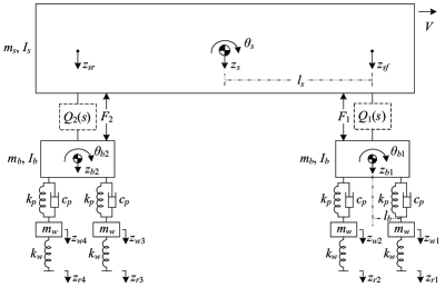
Figure 7: A side-view train suspension model, where the positive-real transfer functions $Q_{1}(s)$ and $Q_{2}(s)$ to be optimized are the admittances of damper-spring-inerter circuits (secondary suspension parts) [12].

By Newton’s Second Law, one can formulate the motion equations as

$$M_{g}\ddot{z}_{g}+C_{g}\dot{z}_{g}+K_{g}z_{g}=E_{g}u+K_{r}z_{r},$$ (36)

where $z_{g}=\left[z_{s},\theta_{s},z_{b1},\theta_{b1},z_{b2},\theta_{b2},z_{w1},z_{w2},z_{w3},z_{w4}\right]^{\mathrm{T}}$, $u=\left[F_{1},F_{2}\right]^{\mathrm{T}}$, $z_{r}=\left[z_{r1},z_{r2},z_{r3},z_{r4}\right]^{\mathrm{T}}$, and the matrices $M_{g}\in\mathbb{R}^{10\times 10}$, $C_{g}\in\mathbb{R}^{10\times 10}$, $K_{g}\in\mathbb{R}^{10\times 10}$, $E_{g}\in\mathbb{R}^{10\times 2}$, and $K_{r}\in\mathbb{R}^{10\times 4}$ are shown in [58, Section V]. By letting $x_{m}=\left[z_{g}^{\mathrm{T}},\dot{z}_{g}^{\mathrm{T}}\right]^{\mathrm{T}}$, equation (36) can be equivalent to

$$\dot{x}_{m}=A_{m}x_{m}+B_{m}u+B_{mw}z_{r},$$ (37)

where

$$\begin{split}A_{m}=\left[\begin{array}[]{cc}\mathbf{0}&I\\ -M_{g}^{-1}K_{g}&-M_{g}^{-1}C_{g}\\ \end{array}\right],~{}B_{m}=\left[\begin{array}[]{c}\mathbf{0}\\ M_{g}^{-1}E_{g}\\ \end{array}\right],~{}B_{mw}=\left[\begin{array}[]{c}\mathbf{0}\\ M_{g}^{-1}K_{r}\\ \end{array}\right].\end{split}$$

Let $w=z_{r1}$. Then, it is clear that $z_{r2}(t)=w(t-\tau_{2})$, $z_{r3}(t)=w(t-\tau_{3})$, and $z_{r4}(t)=w(t-\tau_{4})$, where $\tau_{2}=2l_{b}/V$, $\tau_{3}=2l_{s}/V$, and $\tau_{4}=2(l_{b}+l_{s})/V$. Then, by making use of the Padé approximation method, the minimal state-space realization of the transfer function from $w$ to $z_{r}$ can be obtained as

$$\begin{split}\dot{x}_{r}=A_{r}x_{r}+B_{r}w,~{}~{}z_{r}=C_{r}x_{r}+D_{r}w,\end{split}$$ (38)

where the dimension of $x_{r}\in\mathbb{R}^{n_{r}}$ is based on the order of the Padé approximation. By (36)–(38), the state-space equations are obtained in the form of (A.1), that is,

$$\begin{split}\dot{x}&=Ax+Bu+B_{w}w,\\ y&=Cx,~{}~{}z=C_{z}x,\end{split}$$ (39)

where $x=\left[x_{m}^{\mathrm{T}},x_{r}^{\mathrm{T}}\right]^{\mathrm{T}}$, $z=\left[\dot{z}_{s},\dot{z}_{sf},\dot{z}_{sr}\right]^{\mathrm{T}}$, $y=\left[z_{sf}-z_{b1},z_{sr}-z_{b2},\dot{z}_{sf}-\dot{z}_{b1},\dot{z}_{sr}-\dot{z}_{b2}\right]^{\mathrm{T}}$, and

$$\begin{split}A=\left[\begin{array}[]{cc}A_{m}&B_{mw}C_{r}\\ \mathbf{0}&A_{r}\\ \end{array}\right],~{}~{}B=\left[\begin{array}[]{c}B_{m}\\ \mathbf{0}\\ \end{array}\right],~{}~{}B_{w}=\left[\begin{array}[]{c}B_{mw}D_{r}\\ B_{r}\\ \end{array}\right],\\ C=\left[\begin{array}[]{ccc}C_{11}&\mathbf{0}&\mathbf{0}_{1\times n_{r}}\\ \mathbf{0}&C_{11}&\mathbf{0}_{1\times n_{r}}\\ \end{array}\right],~{}~{}C_{z}=\left[\begin{array}[]{cccc}\mathbf{0}_{1\times 10}&1&0&\mathbf{0}_{1\times(n_{r}+8)}\\ \mathbf{0}_{1\times 10}&1&l_{s}&\mathbf{0}_{1\times(n_{r}+8)}\\ \mathbf{0}_{1\times 10}&1&-l_{s}&\mathbf{0}_{1\times(n_{r}+8)}\\ \end{array}\right],\end{split}$$

with

$$C_{11}=\left[\begin{array}[]{ccccccc}1&l_{s}&-1&0&0&0&\mathbf{0}_{1\times 4}\\ 1&-l_{s}&0&0&-1&0&\mathbf{0}_{1\times 4}\\ \end{array}\right].$$

Furthermore, let the admittances of two secondary suspension circuits satisfy $Q_{1}(s)=Q_{2}(s)$ and be as in (1), that is,

$$Q_{1}(s)=Q_{2}(s)=\frac{\alpha_{3}s^{3}+\alpha_{2}s^{2}+\alpha_{1}s+\alpha_{0}}{\beta_{3}s^{3}+\beta_{2}s^{2}+\beta_{1}s},$$

where the coefficients satisfy Assumption 1. Then, by (A.4), the passive controller $K(s)$ can be obtained as

$$K(s)=\left[\begin{array}[]{cccc}\alpha_{0}/\beta_{1}&&Q_{1,1}(s)&\\ &\alpha_{0}/\beta_{1}&&Q_{2,1}(s)\end{array}\right],$$

where

$$Q_{i,1}(s)=Q_{i}(s)-\frac{\alpha_{0}}{\beta_{1}s}=\frac{\alpha_{2}^{\prime}s^{2}+\alpha_{1}^{\prime}s+\alpha_{0}^{\prime}}{\beta_{3}s^{2}+\beta_{2}s+\beta_{1}}$$

with $\alpha_{2}^{\prime}=\alpha_{3}$ and $\alpha_{j}^{\prime}=(\alpha_{j+1}\beta_{1}-\alpha_{0}\beta_{j+2})/\beta_{1}$ for $i=1,2$ and $j=0,1$. Furthermore, by (A.6), one can formulate a minimal state-space realization of $K(s)$ as in (A.5), that is,

$$\dot{x}_{k}=A_{k}x_{k}+B_{k}y,~{}~{}u=C_{k}x_{k}+D_{k}y,$$ (40)

where $\{A_{k},B_{k},C_{k},D_{k}\}$ satisfy

$$\begin{split}A_{k}=\left[\begin{array}[]{cccc}0&1&0&0\\ -\displaystyle\frac{\beta_{1}}{\beta_{3}}&-\displaystyle\frac{\beta_{2}}{\beta_{3}}&0&0\\ 0&0&0&1\\ 0&0&-\displaystyle\frac{\beta_{1}}{\beta_{3}}&-\displaystyle\frac{\beta_{2}}{\beta_{3}}\\ \end{array}\right],~{}B_{k}=\left[\begin{array}[]{cccc}0&0&0&0\\ 0&0&1&0\\ 0&0&0&0\\ 0&0&0&1\\ \end{array}\right],\\ C_{k}=\left[\begin{array}[]{cccc}\gamma_{0}&\gamma_{1}&0&0\\ 0&0&\gamma_{0}&\gamma_{1}\\ \end{array}\right],~{}D_{k}=\left[\begin{array}[]{cccc}\displaystyle\frac{\alpha_{0}}{\beta_{1}}&0&\displaystyle\frac{\alpha_{3}}{\beta_{3}}&0\\ 0&\displaystyle\frac{\alpha_{0}}{\beta_{1}}&0&\displaystyle\frac{\alpha_{3}}{\beta_{3}}\\ \end{array}\right]\end{split}$$

with $\gamma_{0}=(-\alpha_{0}\beta_{2}\beta_{3}+\alpha_{1}\beta_{1}\beta_{3}-\alpha_{3}\beta_{1}^{2})/(\beta_{1}\beta_{3}^{2})$ and $\gamma_{1}=(-\alpha_{0}\beta_{3}^{2}+\alpha_{2}\beta_{1}\beta_{3}-\alpha_{3}\beta_{1}\beta_{2})/(\beta_{1}\beta_{3}^{2})$. Finally, by (39) and (40), one obtains the closed-loop state-space equations in the form of (A.7), that is,

$$\dot{x}_{cl}=A_{cl}x_{cl}+B_{cl}w,~{}~{}z=C_{cl}x_{cl},$$ (41)

where $x_{cl}=[x^{\mathrm{T}},x_{k}^{\mathrm{T}}]^{\mathrm{T}}$, and $A_{cl}$, $B_{cl}$, and $C_{cl}$ satisfy (A.8), that is,

$$\begin{split}A_{cl}=\left[\begin{array}[]{cc}A+BD_{k}C&BC_{k}\\ B_{k}C&A_{k}\\ \end{array}\right],~{}~{}B_{cl}=\left[\begin{array}[]{c}B_{w}\\ \mathbf{0}\\ \end{array}\right],~{}~{}C_{cl}=\left[\begin{array}[]{cc}C_{z}&\mathbf{0}\end{array}\right].\end{split}$$

Let $S_{\dot{z}}(j\omega)$ and $S_{\dot{w}}(j\omega)$ denote the power spectral density (PSD) function of $\dot{z}$ and $\dot{w}$, respectively. By [12], assume that $\dot{w}=\dot{z}_{r1}$ is a white noise and the corresponding PSD function satisfies $S_{\dot{w}}(j\omega)=4\pi^{2}\kappa V$, where $\kappa$ denotes the vertical track roughness factor. The ride comfort performance measure index $J_{1}$ can be expressed in terms of the root-mean-square (RMS) of $\dot{z}=\left[\ddot{z}_{s},\ddot{z}_{sf},\ddot{z}_{sr}\right]^{\mathrm{T}}$, which by [52] can be equivalent to the $\mathcal{H}_{2}$ norm of the transfer matrix from $w$ to $z$, that is,

$$\begin{split}J_{1}&=\sqrt{\lim_{T\rightarrow\infty}\frac{1}{2T}\int_{-T}^{T}\|\dot{z}(t)\|^{2}dt}=\sqrt{\frac{1}{2\pi}\int_{-\infty}^{\infty}\text{Trace}(S_{\dot{z}}(j\omega))d\omega}\\ &=2\pi\sqrt{\frac{\kappa V}{2\pi}\int_{-\infty}^{\infty}\text{Trace}(H^{\mathrm{T}}_{\dot{w}\rightarrow\dot{z}}(-j\omega)H_{\dot{w}\rightarrow\dot{z}}(j\omega))d\omega}\\ &=2\pi\sqrt{\kappa V}\|H_{w\rightarrow z}\|_{2},\end{split}$$

where $H_{\dot{w}\rightarrow\dot{z}}$ denotes the transfer matrix from $\dot{w}$ to $\dot{z}$ and $H_{w\rightarrow z}$ denotes the transfer matrix from $w$ to $z$ for the closed-loop system in (41), satisfying $H_{\dot{w}\rightarrow\dot{z}}=H_{w\rightarrow z}=C_{cl}(sI-A_{cl})^{-1}B_{cl}$.

By referring to [12, 16], set the parameters as $m_{s}=38000$ kg, $m_{b}=2500$ kg, $m_{w}=1117.9$ kg, $I_{s}=2.31\times 10^{6}$ kgm², $I_{b}=1500$ kgm², $l_{s}=9.5$ m, $l_{b}=1.25$ m, $k_{p}=4.935\times 10^{6}$ N/m, $k_{w}=1\times 10^{6}$ N/m, $c_{p}=5.074\times 10^{4}$ Ns/m, $V=55$ m/s, and $\kappa=2.5\times 10^{-7}$ m³/cycle. Furthermore, utilize the third-order Padé approximation to obtain (38). By following Procedure A.1 and utilizing the optimization solver patternsearch in MATLAB, one can obtain the optimal values of $J_{1}$ (solid line in Fig. 8) and the corresponding optimal positive-real admittances $Q_{1}(s)=Q_{2}(s)$, where the value of static stiffness $k_{s}$ is fixed and ranges from $0.5\times 10^{6}$ N/m to $10\times 10^{6}$ N/m. In the optimization, the objective function can be expressed as $J_{1}^{2}/(4\pi^{2}\kappa V)=\text{Trace}(C_{cl}PC_{cl}^{\mathrm{T}})$, where $P$ is the positive definite matrix solved from the Lyapunov equation $A_{cl}P+PA_{cl}^{\mathrm{T}}+B_{cl}B_{cl}^{\mathrm{T}}=0$, $A_{cl}$ is constrained to be stable, and $Q_{1}(s)=Q_{2}(s)$ is constrained to be a positive-real admittance in (1), whose coefficients satisfy the condition in Lemma 1. In comparison, the optimal performances corresponding to the case when each of the admittances $Q_{1}(s)=Q_{2}(s)$ is realizable as the parallel circuit of one spring and one damper are also presented (dot-dashed line in Fig. 8). As shown in Fig. 8, the ride comfort performance $J_{1}$ can be significantly improved by using the positive-real admittance as in (1), which can also show that introducing inerters can certainly improve system performances.

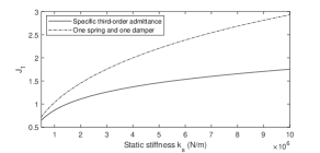
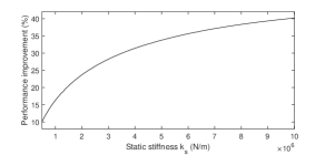
Figure 8: (a) The optimal ride comfort performances $J_{1}$ for the case when each of the admittances $Q_{1}(s)=Q_{2}(s)$ is in the form of (1) (solid line) and the case when each of the admittances $Q_{1}(s)=Q_{2}(s)$ is realizable by the two-element parallel circuit of one spring and one damper (dot-dashed line); (b) the optimal performance improvement in (a), which is $(J_{1}^{(2)}-J_{1}^{(1)})/J_{1}^{(2)}\times 100\%$, where $J_{1}^{(1)}$ and $J_{1}^{(2)}$ are optimal performance values corresponding to the above two cases, respectively. Here, the static stiffness $k_{s}$ ranges from $0.5\times 10^{6}$ N/m to $10\times 10^{6}$ N/m.

Example 3

When $k_{s}=4\times 10^{6}$ N/m, the optimal performance satisfies $J_{1}=1.3722$ and the corresponding positive-real admittance $Q_{1}(s)=Q_{2}(s)$ is in the form of (1) where $\alpha_{3}=3.905\times 10^{7}$, $\alpha_{2}=1.647\times 10^{8}$, $\alpha_{1}=2.93\times 10^{9}$, $\alpha_{0}=k_{s}\beta_{1}=4\times 10^{6}$, $\beta_{3}=41.181$, $\beta_{2}=732.533$, and $\beta_{1}=1$. It is verified that $Q_{1}(s)=Q_{2}(s)$ does not satisfy any of the conditions in Lemma 4, which means that $Q_{1}(s)=Q_{2}(s)$ cannot be realized by a one-port six-element series-parallel circuit by completely removing the pole at $s=0$. It can be checked that $Q_{1}(s)=Q_{2}(s)$ satisfies any of the conditions in Lemmas 6–8, which means that $Q_{1}(s)=Q_{2}(s)$ can be realized by one of the six-element circuit configurations in Fig. 3. For instance, by the element value expressions in (9) with $x=2.413\times 10^{11}$, $Q_{1}(s)$ and $Q_{2}(s)$ can be realized as the circuit in Fig. 3 with $c_{1}=1.177$ Ns/m, $c_{2}=9.484\times 10^{5}$ Ns/m, $k_{1}=3.9997\times 10^{6}$ N/m, $k_{2}=809.474$ N/m, $k_{3}=485.188$ N/m, and $b_{1}=53314.9$ kg. In comparison, by utilizing the Bott-Duffin circuit synthesis procedure, $Q_{1}(s)=Q_{2}(s)$ is realizable by a one-port ten-element series-parallel circuit as shown in Fig. 9 with $c_{1}=8.701\times 10^{6}$ Ns/m, $c_{2}=1.355\times 10^{5}$ Ns/m, $c_{3}=1.064\times 10^{6}$ Ns/m, $k_{1}=k_{s}=4\times 10^{6}$ N/m, $k_{2}=182.143$ N/m, $k_{3}=4.206\times 10^{6}$ N/m, $k_{4}=7.583\times 10^{6}$ N/m, $c_{1}=8.701\times 10^{6}$ Ns/m, $c_{2}=1.355\times 10^{5}$ Ns/m, and $c_{3}=1.064\times 10^{6}$ Ns/m. Therefore, the results of this paper can save four elements for each mechanical circuit realization.

Remark 2

The circuit synthesis results of this paper can guarantee that the six-element series-parallel damper-spring-inerter circuit realizations in Examples 1–3 contain the minimal number of elements. In most cases, if a given admittance satisfies one of the realizability conditions in this paper, any of the corresponding circuit realizations cannot be equivalent to another circuit containing fewer elements by other circuit synthesis approaches.

Figure 9: (a) The one-port six-element series-parallel circuit realizing the optimal positive-real admittances $Q_{1}(s)$ and $Q_{2}(s)$ in Example 3, which is the configuration in Figure 3; (b) the one-port ten-element series-parallel circuit realizing $Q_{1}(s)$ and $Q_{2}(s)$ in Example 3 by making use of the Bott-Duffin circuit synthesis procedure.

6 Conclusion

This paper has solved the passive circuit synthesis problem for a bicubic (third-order) admittance with a simple pole at the origin to be realizable by a one-port series-parallel damper-spring-inerter circuit consisting of at most six elements. Necessary and sufficient conditions have been derived for such a specific bicubic admittance to be realizable as this class of passive circuits, where the conditions are related to the function coefficients and the roots of certain algebraic equations. Moreover, a group of circuit configurations that can realize the admittances satisfying the conditions have been presented, where the element value expressions are explicitly given. Compared with the Bott-Duffin circuit synthesis procedure, much fewer elements are needed to achieve the circuit realizations by using the results of this paper. Finally, numerical examples and the control system design for a train suspension system have been presented. The results derived in this paper can be applied to design and to realize the passive controllers in many inerter-based control systems, and can contribute to the development of passive circuit synthesis and many other related fields.

Appendix A Inerter-Based Mechanical Control Using Passive Controllers

In this appendix, the design procedure of a general class of inerter-based control systems will be formulated. There are $m$ positive-real admittances with a pole at $s=0$, which constitute the passive controller to be determined such that the closed-loop system is stable and the system performance is optimized.

Consider the augmented model of a linear time-invariant vibration system $G(s)$ to be controlled, such as a suspension system, wind turbine vibration system, building vibration system, etc., whose state-space equations are

$$\begin{split}\dot{x}&=Ax+Bu+B_{w}w,\\ y&=Cx,~{}~{}z=C_{z}x,\end{split}$$ (A.1)

where $x$ denotes the state vector, $u$ denotes the input vector consisting of forces provided by passive mechanical circuits, $y$ denotes the measured output for control, $z$ is the controlled output related to system performances, and $w$ denotes the noise vector.

Suppose that there are $m$ one-port spring-damper-inerter circuits, and the admittance of each circuit is positive-real and contains a pole at $s=0$, which is expressed as

$$Q_{i}(s)=\frac{\alpha_{i,n_{i}}s^{n_{i}}+\alpha_{i,n_{i}-1}s^{n_{i}-1}+\cdots+\alpha_{i,1}s+\alpha_{i,0}}{\beta_{i,n_{i}}s^{n_{i}}+\beta_{i,n_{i}-1}s^{n_{i}-1}+\cdots+\beta_{i,1}s}=\frac{\alpha_{i,0}}{\beta_{i,1}s}+Q_{i,1}(s),$$ (A.2)

for $i=1,2,\ldots,m$, where

$$Q_{i,1}(s)=\frac{\alpha_{i,n_{i}-1}^{\prime}s^{n_{i}-1}+\alpha_{i,n_{i}-2}^{\prime}s^{n_{i}-2}+\cdots+\alpha_{i,0}^{\prime}}{\beta_{i,n_{i}}s^{n_{i}-1}+\beta_{i,n_{i}-1}s^{n_{i}-2}+\cdots+\beta_{i,1}}$$ (A.3)

is also a positive-real function with

$$\alpha_{i,n_{i}-1}^{\prime}=\alpha_{i,n_{i}},~{}~{}~{}\alpha_{i,j}^{\prime}=\frac{\alpha_{i,j+1}\beta_{i,1}-\alpha_{i,0}\beta_{i,j+2}}{\beta_{i,1}},$$

for $j=0,1,\ldots,n_{i}-2$.

Then, one aims to design an inerter-based control system whose diagram is as shown in Fig. 10, where the above $m$ admittances constitute the passive controller $K(s)$.

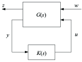
Figure 10: Control synthesis diagram, where $G(s)$ is the transfer (function) matrix of the vibration system (A.1) to be controlled, $K(s)$ is the passive controller, $y$ is the measured output, $u$ is the control input, $w$ is the noise signal, and $z$ is the controlled output.

Let the measured output $y=\left[y_{1}^{\mathrm{T}},y_{2}^{\mathrm{T}}\right]^{\mathrm{T}}\in\mathbb{R}^{2m}$ consist of the relative displacements $y_{1}\in\mathbb{R}^{m}$ and the relative velocities $y_{2}\in\mathbb{R}^{m}$ of two terminals for $m$ circuits. Referring to [13], the $m$ passive circuits $Q_{i}(s)$ as in (A.2) for $i=1,2,\ldots,m$ can constitute the passive controller $K(s)$ whose input is $y$ and output is the force $u$ as in (A.1), that is, $u=K(s)y$. Here, the controller $K(s)$ can be expressed as

$$K(s)=\left[\begin{array}[]{ccc;{2pt/2pt}ccc}\displaystyle\frac{\alpha_{1,0}}{\beta_{1,1}}&&&Q_{1,1}&&\\ &\ddots&&&\ddots&\\ &&\displaystyle\frac{\alpha_{m,0}}{\beta_{m,1}}&&&Q_{m,1}\end{array}\right],$$ (A.4)

with $Q_{i,1}(s)$ for $i=1,2,\ldots,m$ being expressed as in (A.3). Assume that $Q_{i,1}(s)$ for $i=1,2,\ldots,m$ as in (A.3) does not contain any common factor. Based on the results in [1], a minimal state-space realization $\{A_{q_{i}},B_{q_{i}},C_{q_{i}},D_{q_{i}}\}$ of the positive-real function $Q_{i,1}(s)$ for $i=1,2,\ldots,m$ can be obtained as

$$\begin{split}&A_{q_{i}}=\left[\begin{array}[]{cccc}0&1&\cdots&0\\ \vdots&\vdots&\ddots&\vdots\\ 0&0&\cdots&1\\ -\displaystyle\frac{\beta_{i,1}}{\beta_{i,n_{i}}}&-\displaystyle\frac{\beta_{i,2}}{\beta_{i,n_{i}}}&\cdots&-\displaystyle\frac{\beta_{i,n_{i}-1}}{\beta_{i,n_{i}}}\end{array}\right],B_{q_{i}}=\left[\begin{array}[]{c}0\\ \vdots\\ 0\\ 1\end{array}\right],\\ &~{}~{}C_{q_{i}}=\left[\begin{array}[]{cccc}\gamma_{i,0}&\gamma_{i,1}&\cdots&\gamma_{i,n_{i}-2}\end{array}\right],~{}~{}D_{q_{i}}=\left[\begin{array}[]{c}\displaystyle\frac{\alpha_{i,n_{i}}}{\beta_{i,n_{i}}}\end{array}\right],\end{split}$$

where

$$\gamma_{i,k}=\frac{\alpha_{i,k}^{\prime}\beta_{i,n_{i}}-\alpha_{i,n_{i}-1}^{\prime}\beta_{i,k+1}}{\beta_{i,n_{i}}^{2}}=\frac{(\alpha_{i,k+1}\beta_{i,1}-\alpha_{i,0}\beta_{i,k+2})\beta_{i,n_{i}}-\alpha_{i,n_{i}}\beta_{i,1}\beta_{i,k+1}}{\beta_{i,1}\beta_{i,n_{i}}^{2}},$$

for $k=0,1,\ldots,n_{i}-2$. Furthermore, a minimal state-space realization $\{A_{k},B_{k},C_{k},D_{k}\}$ of the controller $K(s)$ as in (A.4) satisfies

$$\begin{split}\dot{x}_{k}=A_{k}x_{k}+B_{k}y,~{}~{}u=C_{k}x_{k}+D_{k}y,\end{split}$$ (A.5)

where the dimension of $x_{k}$ is equal to the McMillan degree of $K(s)$, and $A_{k}$, $B_{k}$, $C_{k}$, and $D_{k}$ are expressed as

$$\begin{split}A_{k}=\left[\begin{array}[]{ccc}A_{q_{1}}&&\\ &\ddots&\\ &&A_{q_{m}}\end{array}\right],~{}~{}B_{k}=\left[\begin{array}[]{ccc;{2pt/2pt}ccc}\mathbf{0}&&&B_{q_{1}}&&\\ &\ddots&&&\ddots&\\ &&\mathbf{0}&&&B_{q_{m}}\end{array}\right],\\ C_{k}=\left[\begin{array}[]{ccc}C_{q_{1}}&&\\ &\ddots&\\ &&C_{q_{m}}\end{array}\right],~{}~{}D_{k}=\left[\begin{array}[]{ccc;{2pt/2pt}ccc}\displaystyle\frac{\alpha_{1,0}}{\beta_{1,1}}&&&D_{q_{1}}&&\\ &\ddots&&&\ddots&\\ &&\displaystyle\frac{\alpha_{m,0}}{\beta_{m,1}}&&&D_{q_{m}}\end{array}\right].\end{split}$$ (A.6)

Combining (A.1) and (A.5), the closed-loop state-space equation can be obtained as

$$\begin{split}\dot{x}_{cl}=A_{cl}x_{cl}+B_{cl}w,~{}~{}z=C_{cl}x_{cl},\end{split}$$ (A.7)

where $x_{cl}=[x^{\mathrm{T}},x_{k}^{\mathrm{T}}]^{\mathrm{T}}$, and

$$A_{cl}=\left[\begin{array}[]{cc}A+BD_{k}C&BC_{k}\\ B_{k}C&A_{k}\\ \end{array}\right],~{}~{}B_{cl}=\left[\begin{array}[]{c}B_{w}\\ \mathbf{0}\\ \end{array}\right],~{}~{}C_{cl}=\left[\begin{array}[]{cc}C_{z}&\mathbf{0}\end{array}\right].$$ (A.8)

Let $H_{w\rightarrow z}(s)=C_{cl}(sI-A_{cl})^{-1}B_{cl}$ denote the transfer (function) matrix from $w$ to $z$. Then, suppose that a system performance is proportional to the $\mathcal{H}_{2}$ norm of $H_{w\rightarrow z}(s)$, that is,

$$J_{\mathrm{passive}}\propto\|H_{w\rightarrow z}\|_{2}.$$ (A.9)

It is implied from [52, Lemma 4.6] that $\|H_{w\rightarrow z}\|_{2}^{2}=\text{Trace}(C_{cl}PC_{cl}^{\mathrm{T}})$, where the positive definite matrix $P>0$ is the unique solution of the Lyapunov equation

$$A_{cl}P+PA_{cl}^{\mathrm{T}}+B_{cl}B_{cl}^{\mathrm{T}}=0.$$ (A.10)

The optimization design procedure for $J_{\mathrm{passive}}$ can be summarized as follows.

Procedure A.1

Consider a vibration system whose state-space equation satisfies (A.1). Then, the steps of designing a passive controller $K(s)$ to minimize the system performance $J_{\mathrm{passive}}\propto\|H_{w\rightarrow z}\|_{2}$ are as follows.

1. Choosing the McMillan degrees of admittances $Q_{i}(s)$ in (A.2) for $i=0,1,\ldots,m$, $K(s)$ can be formulated as in (A.4). Determine the positive-real conditions and further choose the constraint conditions of $Q_{i}(s)$ such that $Q_{i}(s)$ is realizable as a specific class of passive spring-damper-inerter circuits, where the coefficients of $Q_{i}(s)$ are optimization variables.

2. Formulate a minimal state-space realization $\{A_{k},B_{k},C_{k},D_{k}\}$ of $K(s)$ by (A.6).

3. Formulate $A_{cl}$, $B_{cl}$, and $C_{cl}$ by (A.8).

4. Solve the following optimization problem to determine the optimal $J_{\mathrm{passive}}$ and the positive-real admittances $Q_{i}(s)$ for $i=1,2,\ldots,m$:

   $$\begin{split}&\min_{\alpha_{i,j},\beta_{i,k}}~{}\|H_{w\rightarrow z}\|_{2}^{2}=\text{Trace}(C_{cl}PC_{cl}^{\mathrm{T}})\\ &~{}\text{s.t.}~{}~{}A_{cl}~{}\text{is stable}\\ &~{}~{}~{}~{}~{}~{}P>0~{}\text{is the solution of \eqref{eq: Lyapunov equation}}\\ &~{}~{}~{}~{}~{}~{}Q_{i}(s)~{}\text{is a class of positive-real functions in Step~{}1}.\end{split}$$

5. By utilizing the results of passive circuit synthesis, realize the positive-real functions $Q_{i}(s)$ for $i=1,2,\ldots,m$ corresponding to the optimal performance as the admittances of the required spring-damper-inerter circuits.

Remark A.1

By properly modifying the objective function, Procedure A.1 can be similarly applied to the control system design when the system performances are in other forms, such as the $\mathcal{H}_{\infty}$ norm of transfer functions, the weighting sum of multiple performances, etc.

As shown in Procedure A.1, the circuit synthesis results can be utilized as the further optimization constraints in Step 4 and can be utilized to physically realize the positive-real admittances as passive mechanical circuits in Step 5. Therefore, it is both theoretically and practically significant to solve the realization problems of positive-real admittances in the form of (A.2) as passive mechanical circuits containing the least number of elements, where this paper investigates the low-complexity passive circuit synthesis problem when the McMillan degree of the admittance in (A.2) is three.

Appendix B Proof of Lemma 5

To prove Lemma 5, the following lemmas are presented.

Lemma B.1

For any admittance $Y(s)$ in (1) that satisfies Assumption 1 and does not satisfy the conditions of Lemma 4, if $Y(s)$ can be realized by the one-port series-parallel damper-spring-inerter circuit containing at most six elements as in Fig. 1, which satisfies Assumption 2, then the graph of the subcircuit $N_{2}$ must have $k$-$\mathcal{P}(a,a^{\prime})$ and cannot have any of $b$-$\mathcal{P}(a,a^{\prime})$, $k$-$\mathcal{C}(a,a^{\prime})$, or $b$-$\mathcal{C}(a,a^{\prime})$.

Proof: The assumption that the conditions of Lemma 4 do not hold implies that the admittance (or impedance) of circuit $N_{2}$ is not in the biquadratic form, which is obtained by the partial removal of the pole of $Y(s)$ at $s=0$. Therefore, it is implied that $k_{1}\in(0,\alpha_{0}/\beta_{1})$. Then, the admittance of $N_{2}$ is also in the form of (1) with all the coefficients being positive, which has a pole at $s=0$, does not have any pole at $s=\infty$, and does not have any zero at $s=0$ or $s=\infty$. By Lemma 2, one can prove this lemma. $\blacksquare$

Lemma B.2

For any admittance $Y(s)$ in (1) that satisfies Assumption 1 and does not satisfy the conditions of Lemma 4, if $Y(s)$ can be realized by a one-port series-parallel damper-spring-inerter circuit containing at most six elements as in Fig. 1, then the subcircuit $N_{2}$ cannot contain at most two types of elements.

Proof: As shown in the proof of Lemma B.1, the admittance $Y_{2}(s)$ of $N_{2}$ is also in the form of (1) with positive coefficients. Therefore, it is clear that $N_{2}$ contains at least two types of elements. By Lemma 3, $N_{2}$ cannot be a spring-inerter circuit. By Lemma B.1, the requirement of $k$-$\mathcal{P}(a,a^{\prime})$ implies that $N_{2}$ cannot be a damper-inerter circuit.

Assume that $N_{2}$ is a damper-spring circuit. Then, $Y_{2}(s)$ can be in the form of $Y_{2}(s)=H(s+z_{1})(s+z_{2})(s+z_{3})/(s(s+p_{1})(s+p_{2}))$ where $H>0$ and $0<z_{1}<p_{1}<z_{2}<p_{2}<z_{3}$ [53, Chapter 6]. By the second Foster form [53, Chapter 6], $Z_{3}(s)=1/(Y_{2}(s)-k_{2}/s)=1/(H_{1}/(s+p_{1})+H_{2}/(s+p_{2})+H_{3})$ is a positive-real biquadratic impedance that can be realized by a damper-spring circuit, where $k_{2}$ is the residue of $Y_{2}(s)$ at $s=0$. Furthermore, by [27, Lemma 7], $Z_{3}(s)$ is regular. Therefore, Condition 1 of Lemma 4 holds, which contradicts the assumption. $\blacksquare$

Lemma B.3

Any admittance $Y(s)$ in (1) satisfying Assumption 1 cannot be realized by the one-port circuit configuration in Fig. 11(a).

Proof: The admittance of the circuit in Fig. 11(a) is calculated as $Y(s)=n(s)/d(s)$ where $n(s)=b_{1}b_{2}c_{1}s^{4}+b_{1}b_{2}(k_{1}+k_{3})s^{3}+c_{1}(b_{1}k_{1}+b_{1}k_{3}+b_{2}k_{1}+b_{2}k_{2})s^{2}+b_{2}(k_{1}k_{2}+k_{1}k_{3}+k_{2}k_{3})s+c_{1}(k_{1}k_{2}+k_{1}k_{3}+k_{2}k_{3})$ and $d(s)=b_{1}b_{2}s^{4}+c_{1}(b_{1}+b_{2})s^{3}+b_{2}(k_{2}+k_{3})s^{2}+c_{1}(k_{2}+k_{3})s$. Then, the resultant of $n(s)$ and $d(s)$ in $s$ is calculated as $R_{0}(n,d,s)=b_{1}b_{2}c_{1}^{4}(k_{1}k_{2}+k_{1}k_{3}+k_{2}k_{3})(c_{1}^{2}(b_{1}k_{3}-b_{2}k_{2})^{2}+b_{1}b_{2}^{2}k_{2}k_{3}^{2})^{2}$, which can never be zero. Thus, the circuit in Fig. 11(a) cannot realize the admittance $Y(s)$ in this lemma, whose McMillan degree is three. $\blacksquare$

Necessity. To prove the necessity part, one will show that any circuit realizing the admittance $Y(s)$ in this lemma can be equivalent to one of the configurations in Fig. 3. Since any one-port circuit whose graph is not connected or whose augmented graph is separable can be equivalent to another circuit satisfying Assumption 2, one only needs to discuss the circuits that satisfies Assumption 2 to avoid repeated discussions.

When the circuit $N_{2}$ is further the series connection of two circuits, by Lemma B.1, $Y(s)$ can be realized by the circuit structure in Fig. 11(b) to guarantee the existence of $k$-$\mathcal{P}(a,a^{\prime})$ and to avoid the existence of $k$-$\mathcal{C}(a,a^{\prime})$, where the springs $k_{2}$ and $k_{3}$ and two subcircuits $N_{3}$ and $N_{4}$ constitute $N_{2}$. Based on the symmetry, assume that $N_{3}$ contains one element and $N_{4}$ contains one or two elements. Then, by Lemmas B.1–B.3, the realization can always be equivalent to one of the configurations in Figs. 3 and 3, where Fig. 3 can represent a five-element configuration when $c_{2}=0$ (open-circuited).

When the circuit $N_{2}$ is further the parallel connection of two circuits, to avoid repeated discussions, one assumes that $N_{2}$ cannot be equivalent to the parallel circuit of a spring and a subcircuit due to the parallel spring $k_{1}$. Therefore, the subcircuit of $N_{2}$ providing the $k$-$\mathcal{P}(a,a^{\prime})$ must contain at least two springs. Furthermore, based on the equivalence in Fig. 12 and by Lemma B.1, the realization of $Y(s)$ can be a circuit whose structure is in Fig. 11(c), where the damper $c_{1}$, springs $k_{2}$ and $k_{3}$, and two subcircuits $N_{3}$ and $N_{4}$ constitute $N_{2}$, and each of $N_{3}$ and $N_{4}$ contains only one element. Furthermore, by Lemmas 3, B.1, and B.2, it is implied that only the circuit in Fig. 3 is possible.

Therefore, the proof of the necessity part has been completed.

Sufficiency. The sufficiency part of this lemma obviously holds.

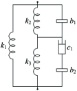
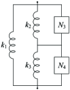
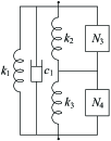
Figure 11: (a) The circuit configuration that cannot realize the admittance $Y(s)$ in Lemma B.3; (b) the realization structure of $Y(s)$ discussed in the proof of Lemma 5, where $k_{2}$, $k_{3}$, $N_{3}$, and $N_{4}$ constitute the circuit $N_{2}$ as in Fig. 1, $N_{3}$ contains one element, and $N_{4}$ contains one or two elements; (c) the realization structure of $Y(s)$ discussed in the proof of Lemma 5, where $c_{1}$, $k_{2}$, $k_{3}$, $N_{3}$, and $N_{4}$ constitute the circuit $N_{2}$ as in Fig. 1, and each of $N_{3}$ and $N_{4}$ contains only one element.

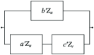
Figure 12: Two equivalent one-port series-parallel passive circuit structures, where $a^{\prime}=a(a+b)/b$, $b^{\prime}=a+b$, $c^{\prime}=c(a+b)^{2}/b^{2}$, and $Z_{u}$ and $Z_{v}$ are positive-real impedances (See [27, Fig. 6]).

Appendix C Proof of Lemma 6

Necessity. The admittance of the circuit configuration in Fig. 3 is computed as $Y(s)=n(s)/d(s)$, where $n(s)=b_{1}c_{1}s^{3}+(b_{1}k_{1}+b_{1}k_{2}+c_{1}c_{2})s^{2}+(c_{1}k_{1}+c_{1}k_{3}+c_{2}k_{1}+c_{2}k_{2})s+k_{1}k_{2}+k_{1}k_{3}+k_{2}k_{3}$ and $d(s)=b_{1}s^{3}+(c_{1}+c_{2})s^{2}+(k_{2}+k_{3})s$. Since $Y(s)$ in (1) satisfying Assumption 1 is realizable by the circuit in Fig. 3, there exists $k>0$ such that $n(s)=k\alpha(s)$ and $d(s)=k\beta(s)$. Then, it follows that

$$b_{1}c_{1} =k\alpha_{3},$$ (C.1a)

$$b_{1}k_{1}+b_{1}k_{2}+c_{1}c_{2} =k\alpha_{2},$$ (C.1b)

$$c_{1}k_{1}+c_{1}k_{3}+c_{2}k_{1}+c_{2}k_{2} =k\alpha_{1},$$ (C.1c)

$$k_{1}k_{2}+k_{1}k_{3}+k_{2}k_{3} =k\alpha_{0},$$ (C.1d)

$$b_{1} =k\beta_{3},$$ (C.1e)

$$c_{1}+c_{2} =k\beta_{2},$$ (C.1f)

$$k_{2}+k_{3} =k\beta_{1},$$ (C.1g)

where $k>0$. Letting

$$x=\frac{\alpha_{3}^{2}}{k\beta_{3}}>0,$$ (C.2)

the expression of $b_{1}$ can be obtained from (C.1e) as in (5). Then, it follows from (C.1a) and (C.1e) that $c_{1}$ can be expressed as in (5), which together with (C.1f) and (C.2) implies that $c_{2}$ can be expressed as in (5). Since $c_{2}\geq 0$, one implies that $x$ satisfies (4b). It follows from (C.1g) and (C.2) that

$$k_{3}=\frac{\alpha_{3}^{2}\beta_{1}}{\beta_{3}x}-k_{2}.$$ (C.3)

Then, substituting (C.1e), (C.3), and the expressions of $c_{1}$, $c_{2}$, and $b_{1}$ shown in (5) into (C.1b) and (C.1c) yields the expressions of $k_{1}$ and $k_{2}$ as in (5), which together with (C.3) implies that $k_{3}$ can be expressed as in (5). By the assumption that $k_{1}>0$, $k_{2}>0$, and $k_{3}>0$, it is implied that $x$ satisfies (4c) and (4d). Furthermore, substituting (C.2) and the expressions of $k_{1}$, $k_{2}$, and $k_{3}$ as in (5) into (C.1d), one implies that $x$ is a positive root of the equation (4a). Now, the proof of the necessity part has been completed.

Sufficiency. Let $c_{1}$, $c_{2}$, $k_{1}$, $k_{2}$, $k_{3}$, and $b_{1}$ satisfy the expressions in (5), where $x$ is a positive root of equation (4a) such that (4b)–(4d). Then, it can be verified that $c_{2}\geq 0$ and other element values are positive and finite. Since (4a) holds, it can be verified that (C.1a)–(C.1g) hold with $k$ satisfying $k=\alpha_{3}^{2}/(\beta_{3}x)$. Therefore, $Y(s)$ can be realized by the circuit in Fig. 3.

Appendix D Proof of Lemma 9

To prove Lemma 9, the following lemmas are presented, which will be utilized for the proof.

Lemma D.1

For any admittance $Y(s)$ in (1) that satisfies Assumption 1 and does not satisfy the conditions of Theorem 1, if $Y(s)$ is realizable as a one-port series-parallel damper-spring-inerter circuit containing at most six elements, then the circuit cannot contain no more than two types of elements.

Proof: The assumption that the conditions of Theorem 1 do not hold implies that the series-parallel realizations of $Y(s)$ containing no more than six elements cannot be as in Fig. 1. Then, this lemma can be proved similar to Lemma B.2. $\blacksquare$

Lemma D.2

For any admittance $Y(s)$ in (1) that satisfies Assumption 1 and does not satisfy the conditions of Theorem 1, if $Y(s)$ is realizable as a one-port series-parallel damper-spring-inerter circuit containing no more than six elements, which satisfies Assumption 2 and is the parallel connection of two subcircuits $N_{1}$ and $N_{2}$, then the subcircuit $N_{2}$ constituting $k$-$\mathcal{P}(a,a^{\prime})$ must contain at least four elements and cannot contain no more than two types of elements.

Proof: Since the conditions of Theorem 1 do not hold, $Y(s)$ cannot be realizable by any circuit as in Fig. 1, which contains at most six elements. Therefore, the subnetwork $N_{2}$ constituting $k$-$\mathcal{P}(a,a^{\prime})$ must contain at least two springs, to avoid the single parallel spring in Fig. 1. Moreover, together with the equivalence in Fig. 12, there must be at least two other elements. Therefore, the total number of elements is at least four. Assume that $N_{2}$ is a damper-spring circuit. Then, similar to the proof of Lemma B.2, this contradicts the assumption that $Y(s)$ cannot be realizable as in Fig. 1 containing no more than six elements. Together with Lemma 3, one can prove that $N_{2}$ cannot contain no more than two types of elements. $\blacksquare$

Lemma D.3

Any admittance $Y(s)$ in (1) satisfying Assumption 1 cannot be realized by any of the circuit configurations in Fig. 13.

Proof: The method of the proof is similar to Lemma B.3. $\blacksquare$

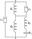
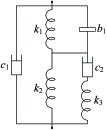
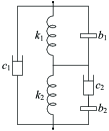
Figure 13: The circuit configurations that cannot realize the admittance $Y(s)$ in Lemma D.3.

Necessity. Similar to the proof of Lemma 5, one will show that any circuit realizing the admittance $Y(s)$ in this lemma can be equivalent to one of the configurations in Figs. 4–5. To avoid repeated discussions, one only needs to discuss the circuits that satisfies Assumption 2.

First, one will investigate the case when the circuit realizing $Y(s)$ is the parallel connection of two subcircuits $N_{1}$ and $N_{2}$. By Lemma 2, at least one of the two subcircuits must constitute $k$-$\mathcal{P}(a,a^{\prime})$, which is assumed to be $N_{2}$. Then, together with Lemmas 2, 3, and D.2, one can imply that the realization can be equivalent to one of the structures in Fig. 14, where $N_{1}$ contains only one element and $N_{2}$ contains one or two elements for the structure in Fig. 14(a), and each of $N_{1}$ and $N_{2}$ contains only one element for each structure in Figs. 14(b) and 14(c). Together with the realization constraints in Lemma 2 and the configurations that cannot realize $Y(s)$ as stated in Lemma D.3, $Y(s)$ is realizable by one of the circuit configurations in Fig. 4 by the method of enumeration.

Then, it turns to discuss the case when the realization of $Y(s)$ is the series connection of two subcircuits $N_{1}$ and $N_{2}$. Here, one can assume that the number of elements in $N_{1}$ is no larger than the number of elements in $N_{2}$ without loss of generality. Thus, $N_{1}$ can only contain one, two, or three elements. By Lemma 2, $N_{1}$ cannot contain only one element, to simultaneously guarantee $k$-$\mathcal{P}(a,a^{\prime})$ and avoid $k$-$\mathcal{C}(a,a^{\prime})$. When $N_{1}$ contain two elements, it is implied that $N_{1}$ can only be the parallel circuit of a damper and a spring, since $N_{1}$ cannot be a spring-inerter circuit by Lemma 3 and $N_{1}$ must contain at least one spring to form $k$-$\mathcal{P}(a,a^{\prime})$. Furthermore, one can prove that $N_{2}$ can only be the parallel connection of two subcircuits. To guarantee $k$-$\mathcal{P}(a,a^{\prime})$ and together with the equivalence in Fig. 12, $N_{2}$ can always be equivalent to the parallel connection of a spring and a subcircuit $N_{3}$, where $N_{3}$ contains two or three elements. The structure is shown in Fig. 14(d). By the method of enumeration and together with Lemmas 3 and D.1, $Y(s)$ is realizable by one of the circuit configurations in Figs. 5–5, where the circuit configuration in Fig. 5 can represent a five-element series-parallel circuit configuration when $c_{2}^{-1}=0$ or $c_{3}=0$ ($c_{2}^{-1}=0$ and $c_{3}=0$ cannot simultaneously hold). Similarly, when $N_{1}$ contain three elements, one can show that any realization of $Y(s)$ can always be equivalent to the structure in Fig. 14(e), where both $N_{3}$ and $N_{4}$ contain two elements. Furthermore, by the method of enumeration and together with Lemmas 3 and D.1, $Y(s)$ is realizable by one of the circuit configurations in Figs. 5 and 5.

Therefore, the necessity part of the proof has been completed.

Sufficiency. The sufficiency part of this lemma obviously holds.

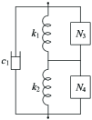
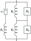
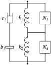
Figure 14: The structures of the circuits realizing $Y(s)$ discussed in the proof of Lemma D.2. For the structure in (a), $N_{3}$ contains only one element, and $N_{4}$ contains two or three elements; for the structures in (b) and (c), each of $N_{3}$ and $N_{4}$ contains one element; for the structure in (d), $N_{3}$ contains two or three elements; for the structure in (e), each of $N_{3}$ and $N_{4}$ contains two elements.

Appendix E Proof of Lemma 12

Necessity. The admittance of the circuit configuration in Fig. 4 is computed as $Y(s)=n(s)/d(s)$, where $n(s)=b_{1}c_{1}c_{2}s^{4}+b_{1}(c_{1}k_{1}+c_{1}k_{2}+c_{2}k_{1})s^{3}+(b_{1}k_{1}k_{2}+c_{1}c_{2}k_{1}+c_{1}c_{2}k_{3})s^{2}+(c_{1}k_{1}k_{2}+c_{1}k_{2}k_{3}+c_{1}k_{1}k_{3}+c_{2}k_{1}k_{3})s+k_{1}k_{2}k_{3}$ and $d(s)=b_{1}c_{1}s^{4}+(b_{1}k_{1}+c_{1}c_{2})s^{3}+(c_{1}k_{2}+c_{1}k_{3}+c_{2}k_{1})s^{2}+k_{1}(k_{3}+k_{3})s$. If the given admittance $Y(s)$ of this lemma is realizable by the circuit in Fig. 4, then the resultant of $n(s)$ and $d(s)$ in $s$ calculated as $R_{0}(n,d,s)=-b_{1}c_{1}^{2}k_{1}^{3}k_{2}k_{3}(b_{1}k_{2}^{2}+c_{2}^{2}k_{3})^{2}(b_{1}k_{1}^{2}+c_{1}^{2}k_{2}+c_{1}^{2}k_{3}-c_{1}c_{2}k_{1})^{2}$ is zero. Therefore, one obtains that $c_{2}$ satisfies the expression in (15), which further implies that the admittance of the configuration in Fig. 4 becomes $Y(s)=\tilde{n}(s)/\tilde{d}(s)$, where $\tilde{n}(s)=b_{1}(b_{1}k_{1}^{2}+k_{2}c_{1}^{2}+k_{3}c_{1}^{2})s^{3}+b_{1}c_{1}k_{1}(k_{1}+k_{2})s^{2}+(k_{3}(b_{1}k_{1}^{2}+c_{1}^{2}k_{2}+c_{1}^{2}k_{3})+c_{1}^{2}k_{1}(k_{2}+k_{3}))s+c_{1}k_{1}k_{2}k_{3}$ and $\tilde{d}(s)=b_{1}c_{1}k_{1}s^{3}+(b_{1}k_{1}^{2}+c_{1}^{2}k_{2}+c_{1}^{2}k_{3})s^{2}+c_{1}k_{1}(k_{2}+k_{3})s$. Therefore, there exists $k>0$ such that $\tilde{n}(s)=k\alpha(s)$ and $\tilde{d}(s)=k\beta(s)$. Then, it follows that

$$b_{1}(b_{1}k_{1}^{2}+k_{2}c_{1}^{2}+k_{3}c_{1}^{2}) =k\alpha_{3},$$ (E.1a)

$$b_{1}c_{1}k_{1}(k_{1}+k_{2}) =k\alpha_{2},$$ (E.1b)

$$k_{3}(b_{1}k_{1}^{2}+c_{1}^{2}k_{2}+c_{1}^{2}k_{3})+c_{1}^{2}k_{1}(k_{2}+k_{3}) =k\alpha_{1},$$ (E.1c)

$$c_{1}k_{1}k_{2}k_{3} =k\alpha_{0},$$ (E.1d)

$$b_{1}c_{1}k_{1} =k\beta_{3},$$ (E.1e)

$$b_{1}k_{1}^{2}+c_{1}^{2}k_{2}+c_{1}^{2}k_{3} =k\beta_{2},$$ (E.1f)

$$c_{1}k_{1}(k_{2}+k_{3}) =k\beta_{1},$$ (E.1g)

where $k>0$. From (E.1a) and (E.1f), it is implied that the value of $b_{1}$ can be expressed as in (15). Let $x$ satisfies

$$x=\beta_{2}(\alpha_{2}-\beta_{3}k_{1}).$$ (E.2)

Then, the expression of $k_{1}$ can be obtained as in (15). Together with (E.2), it is implied from (E.1b) and (E.1e) that $k_{2}$ can be expressed as in (15), which implies that $x>0$. By (E.1e), (E.1g), (E.2), and the expression of $b_{1}$ as in (15), the expression of $k_{3}$ can be derived as in (15). It follows from (E.1d) and (E.1g) that $k_{2}^{-1}+k_{3}^{-1}=\beta_{1}/\alpha_{0}$, which together with the expressions of $k_{2}$ and $k_{3}$ as in (15) implies that

$$x^{2}-\alpha_{3}\beta_{1}x+\alpha_{0}\alpha_{3}\beta_{2}\beta_{3}=0.$$ (E.3)

Therefore, it is clear that (14a) holds and the root of equation (E.3) can be solved as in (14d). Substituting (E.1f) and (E.1g) into (E.1c) implies that $k_{3}\beta_{2}+c_{1}\beta_{1}=\alpha_{1}$, which together with the expressions of $c_{1}$ and $k_{3}$ implies that the value of $c_{1}$ can be expressed as in (15). By the element values of $c_{1}$, $k_{1}$, $k_{2}$, and $k_{3}$, it follows from (E.1g) that

$$k=\frac{\alpha_{3}(\alpha_{2}\beta_{2}-x)(x-\mathcal{B}_{23})}{\beta_{1}\beta_{2}^{2}\beta_{3}^{3}}.$$ (E.4)

Furthermore, by the expressions of $c_{1}$, $k_{1}$, $k_{2}$, $k_{3}$ and $b_{1}$, it follows from (E.1f) that (14b) holds. By the assumption that the element values expressed in (15) are positive and finite, one implies that $x>0$ satisfies (14c). The proof of the necessity part has been completed.

Sufficiency. Let the element values of $c_{1}$, $c_{2}$, $k_{1}$, $k_{2}$, $k_{3}$, and $b_{1}$ satisfy (15), where (14a) holds, and $x$ is a positive root of (14b), such that (14c) and (14d) hold. Then, it can be verified that the element values are positive and finite. Moreover, together with the expression of $c_{2}$ in (15), it can be calculated that the admittance of the configuration in Fig. 4 is $Y(s)=\tilde{n}(s)/\tilde{d}(s)$, where $\tilde{n}(s)=b_{1}(b_{1}k_{1}^{2}+k_{2}c_{1}^{2}+k_{3}c_{1}^{2})s^{3}+b_{1}c_{1}k_{1}(k_{1}+k_{2})s^{2}+(k_{3}(b_{1}k_{1}^{2}+c_{1}^{2}k_{2}+c_{1}^{2}k_{3})+c_{1}^{2}k_{1}(k_{2}+k_{3}))s+c_{1}k_{1}k_{2}k_{3}$ and $\tilde{d}(s)=b_{1}c_{1}k_{1}s^{3}+(b_{1}k_{1}^{2}+c_{1}^{2}k_{2}+c_{1}^{2}k_{3})s^{2}+c_{1}k_{1}(k_{2}+k_{3})s$. Since $x$ satisfies (14b) and (14d), it can be verified that (E.1a)–(E.1g) hold. Therefore, $Y(s)$ is realizable by the circuit in Fig. 4.

References

Kai Wang,  Michael Z. Q. Chen,   and   Fei Liu

1 Introduction

This report presents some supplementary material to the paper entitled “Series-parallel mechanical circuit synthesis of a positive-real third-order admittance using at most six passive elements for inerter-based control” [1], which are omitted from the original paper for brevity. It is assumed that the numbering of lemmas, theorems, equations and figures in this report agrees with that in the original paper.

2 Realizability Conditions of the Configurations in Fig. 3

2.1 The Configuration in Fig. 3(b) (The Proof of Lemma 7)

Necessity. The admittance of the circuit configuration in Fig. 3(b) is calculated as $Y(s)=n(s)/d(s)$, where $n(s)=b_{1}c_{1}c_{2}s^{3}+b_{1}(c_{1}k_{1}+c_{1}k_{3}+c_{2}k_{1}+c_{2}k_{2})s^{2}+(b_{1}k_{1}k_{2}+b_{1}k_{1}k_{3}+b_{1}k_{2}k_{3}+c_{1}c_{2}k_{1}+c_{1}c_{2}k_{3})s+c_{2}(k_{1}k_{2}+k_{2}k_{3}+k_{1}k_{3})$ and $d(s)=b_{1}(c_{1}+c_{2})s^{3}+(b_{1}k_{2}+b_{1}k_{3}+c_{1}c_{2})s^{2}+c_{2}(k_{2}+k_{3})s$. Since $Y(s)$ is realizable by the circuit in Fig. 3(b), there exists $k>0$ such that $n(s)=k\alpha(s)$ and $d(s)=k\beta(s)$. Then, it follows that

$$b_{1}c_{1}c_{2} =k\alpha_{3},$$ (2.1a)

$$b_{1}(c_{1}k_{1}+c_{1}k_{3}+c_{2}k_{1}+c_{2}k_{2}) =k\alpha_{2},$$ (2.1b)

$$b_{1}k_{1}k_{2}+b_{1}k_{1}k_{3}+b_{1}k_{2}k_{3}+c_{1}c_{2}k_{1}+c_{1}c_{2}k_{3} =k\alpha_{1},$$ (2.1c)

$$c_{2}(k_{1}k_{2}+k_{2}k_{3}+k_{1}k_{3}) =k\alpha_{0},$$ (2.1d)

$$b_{1}(c_{1}+c_{2}) =k\beta_{3},$$ (2.1e)

$$b_{1}k_{2}+b_{1}k_{3}+c_{1}c_{2} =k\beta_{2},$$ (2.1f)

$$c_{2}(k_{2}+k_{3}) =k\beta_{1},$$ (2.1g)

where $k>0$. Then, it follows from (2.1a) and (2.1e) that $1/c_{1}+1/c_{2}=\beta_{3}/\alpha_{3}$, which implies the expression of $c_{2}$ as in

$$c_{2}=\frac{\alpha_{3}c_{1}}{\beta_{3}c_{1}-\alpha_{3}}.$$ (2.2)

Furthermore, by (2.1d) and (2.1g), the expression of $k_{3}$ can be obtained as in

$$k_{3}=\frac{k_{2}(\alpha_{0}-\beta_{1}k_{1})}{\beta_{1}(k_{1}+k_{2})-\alpha_{0}}.$$ (2.3)

It follows from (2.1a) and (2.1g) that $(k_{2}+k_{3})/(b_{1}c_{1})=\beta_{1}/\alpha_{3}$, which implies the expression of $b_{1}$ as in

$$b_{1}=\frac{\alpha_{3}k_{2}^{2}}{c_{1}(\beta_{1}(k_{1}+k_{2})-\alpha_{0})},$$ (2.4)

which implies that $\beta_{1}(k_{1}+k_{2})-\alpha_{0}>0$. Substituting (2.2)–(2.4) into (2.1a) yields

$$k=\frac{\alpha_{3}c_{1}k_{2}^{2}}{(\beta_{3}c_{1}-\alpha_{3})(\beta_{1}(k_{1}+k_{2})-\alpha_{0})}.$$ (2.5)

Let

$$x=k_{1}>0,~{}~{}~{}y=k_{2}>0.$$ (2.6)

By (2.2)–(2.4) the element values of $c_{2}$, $k_{3}$, and $b_{1}$ can be further expressed as in (7), which together with (2.1c) and (2.1f) implies that $c_{1}$ can be expressed as in (7). Substituting the element values in (7) and $k$ expressed as in (2.5) into (2.1b) and (2.1c) implies (6a) and (6b), respectively. The assumption that the element values are positive and finite implies that (6c) and (6d) hold. Now, the necessity part is proved.

Sufficiency. Let $c_{1}$, $c_{2}$, $k_{1}$, $k_{2}$, $k_{3}$, and $b_{1}$ satisfy (7), where $x>0$ and $y>0$ are positive roots of the equations in (6a) and (6b) such that (6c) and (6d) hold. Then, it can be verified that the element values are positive and finite. Since (6a) and (6b) hold, it can be verified that (2.1a)–(2.1g) hold with $k$ satisfying (2.5). Therefore, $Y(s)$ is realizable by the circuit in Fig. 3(b).

2.2 The Configuration in Fig. 3(c) (The Proof of Lemma 8)

Necessity. The admittance of the circuit configuration in Fig. 3(c) is calculated as $Y(s)=n(s)/d(s)$ where $n(s)=b_{1}(c_{1}+c_{2})s^{3}+(b_{1}k_{1}+b_{1}k_{2}+c_{1}c_{2})s^{2}+(c_{1}k_{2}+c_{1}k_{3}+c_{2}k_{1}+c_{2}k_{3})s+k_{1}k_{2}+k_{2}k_{3}+k_{1}k_{3}$ and $d(s)=b_{1}s^{3}+c_{2}s^{2}+(k_{2}+k_{3})s$. Since $Y(s)$ is realizable by the circuit in Fig. 3(c), there exists $k>0$ such that $n(s)=k\alpha(s)$ and $d(s)=k\beta(s)$. Then, it follows that

$$b_{1}(c_{1}+c_{2}) =k\alpha_{3},$$ (2.7a)

$$b_{1}k_{1}+b_{1}k_{2}+c_{1}c_{2} =k\alpha_{2},$$ (2.7b)

$$c_{1}k_{2}+c_{1}k_{3}+c_{2}k_{1}+c_{2}k_{3} =k\alpha_{1},$$ (2.7c)

$$k_{1}k_{2}+k_{2}k_{3}+k_{1}k_{3} =k\alpha_{0},$$ (2.7d)

$$b_{1} =k\beta_{3},$$ (2.7e)

$$c_{2} =k\beta_{2},$$ (2.7f)

$$k_{2}+k_{3} =k\beta_{1},$$ (2.7g)

where $k>0$. Substituting (2.7e) and (2.7f) into (2.7a) implies

$$c_{1}=\frac{\alpha_{3}-\beta_{2}\beta_{3}k}{\beta_{3}},$$ (2.8)

which together with (2.7b), (2.7e), and (2.7f) implies that

$$k_{2}=\frac{\beta_{2}^{2}\beta_{3}k-\beta_{3}^{2}k_{1}-\mathcal{B}_{33}}{\beta_{3}^{2}}.$$ (2.9)

Substituting (2.7f)–(2.9) into (2.7c) can imply

$$k_{3}=\frac{\beta_{1}\beta_{2}\beta_{3}k-\beta_{2}\beta_{3}k_{1}-\mathcal{B}_{23}}{\beta_{2}\beta_{3}}.$$ (2.10)

By (2.9) and (2.10), it follows from (2.7g) that

$$k=\frac{2\beta_{2}\beta_{3}^{2}k_{1}+\beta_{3}\mathcal{B}_{23}+\beta_{2}\mathcal{B}_{33}}{\beta_{2}^{3}\beta_{3}}.$$ (2.11)

Letting

$$x=2\beta_{2}\beta_{3}k_{1}>0,$$ (2.12)

it follows from (2.7e), (2.7f), and (2.8)–(2.11) that the values of $c_{1}$, $c_{2}$, $k_{1}$, $k_{2}$, $k_{3}$, and $b_{1}$ can be expressed as in (9). The assumption that the element values are positive and finite implies that $x$ satisfies (8b) and (8c). Finally, substituting the expressions of $k_{1}$, $k_{2}$, and $k_{3}$ as in (9) into (2.7d), it is implied that $x>0$ is a positive root of the equation (8a). Now, the proof of the necessity part has been completed.

Sufficiency. Let the values of $c_{1}$, $c_{2}$, $k_{1}$, $k_{2}$, $k_{3}$, and $b_{1}$ satisfy (9), where $x$ is a positive root of equation (8a) such that (8b) and (8c) hold. Then, it can be verified that all the element values are positive and finite. Since (8a) holds, it can be verified that (2.7a)–(2.7g) hold with $k$ satisfying (2.11). Therefore, $Y(s)$ is realizable by the circuit in Fig. 3(c).

3 Realizability Conditions of the Configurations in Fig. 4

3.1 The Configuration in Fig. 4(a) (The Proof of Lemma 10)

Necessity. The admittance of the circuit configuration in Fig. 4(a) is computed as $Y(s)=n(s)/d(s)$ where $n(s)=b_{1}(c_{1}+c_{2})s^{3}+(b_{1}k_{1}+c_{1}c_{2}+c_{2}c_{3}+c_{1}c_{3})s^{2}+(c_{1}k_{1}+c_{1}k_{2}+c_{2}k_{2}+c_{3}k_{1})s+k_{1}k_{2}$ and $d(s)=b_{1}s^{3}+(c_{2}+c_{3})s^{2}+(k_{1}+k_{2})s$. Since $Y(s)$ can be realized by the circuit in Fig. 4(a), there exists $k>0$ such that $n(s)=k\alpha(s)$ and $d(s)=k\beta(s)$. Then, it follows that

$$b_{1}(c_{1}+c_{2}) =k\alpha_{3},$$ (3.1a)

$$b_{1}k_{1}+c_{1}c_{2}+c_{2}c_{3}+c_{1}c_{3} =k\alpha_{2},$$ (3.1b)

$$c_{1}k_{1}+c_{1}k_{2}+c_{2}k_{2}+c_{3}k_{1} =k\alpha_{1},$$ (3.1c)

$$k_{1}k_{2} =k\alpha_{0},$$ (3.1d)

$$b_{1} =k\beta_{3},$$ (3.1e)

$$c_{2}+c_{3} =k\beta_{2},$$ (3.1f)

$$k_{1}+k_{2} =k\beta_{1},$$ (3.1g)

where $k>0$. Then, it follows from (3.1a) and (3.1e) that $c_{1}+c_{2}=\alpha_{3}/\beta_{3}$, which together with (3.1f) implies that

$$c_{2}=\frac{\alpha_{3}-\beta_{3}c_{1}}{\beta_{3}},~{}~{}~{}c_{3}=\frac{\beta_{2}\beta_{3}k+\beta_{3}c_{1}-\alpha_{3}}{\beta_{3}}.$$ (3.2)

Let $x$ satisfies

$$x=k_{1}>0.$$ (3.3)

From (3.1d) and (3.1g), one obtains

$$k=\frac{x^{2}}{\beta_{1}x-\alpha_{0}},$$ (3.4)

which implies that $\beta_{1}x-\alpha_{0}>0$. Substituting (3.1g) and (3.2)–(3.4) into (3.1c), it is implied that $c_{1}$ can be expressed as in (11). Furthermore, substituting the expression of $k$ in (3.4) into (3.1e), (3.1g), and (3.2), one can obtain the expressions of $b_{1}$, $k_{2}$, $c_{2}$, and $c_{3}$ as in (11). Together with the element value expressions in (11) and the expression of $k$ in (3.4), it follows from (3.1b) that (10a) holds. The assumption that $c_{3}\geq 0$ and other element values are positive and finite implies that $x$ satisfies (10b)–(10d). Now, the proof of the necessity part has been completed.

Sufficiency. Let $c_{1}$, $c_{2}$, $c_{3}$, $k_{1}$, $k_{2}$, and $b_{1}$ satisfy (11), where $x$ is a positive root of equation (10a) such that (10b)–(10d). Then, it can be verified that $c_{3}\geq 0$ and other element values can be positive and finite. Since (10a) holds, one can verify that (3.1a)–(3.1g) hold with $k$ satisfying (3.4). Therefore, $Y(s)$ is realizable by the circuit configuration in Fig. 4(a).

3.2 The Configuration in Fig. 4(b) (The Proof of Lemma 11)

Necessity. The admittance of the circuit configuration in Fig. 4(b) is calculated as $Y(s)=n(s)/d(s)$ where $n(s)=b_{1}(c_{1}c_{2}+c_{2}c_{3}+c_{1}c_{3})s^{3}+(c_{1}(b_{1}k_{1}+b_{1}k_{2}+c_{2}c_{3})+b_{1}(c_{2}k_{2}+c_{3}k_{1}))s^{2}+(b_{1}k_{1}k_{2}+c_{1}c_{3}k_{1}+c_{1}c_{3}k_{2}+c_{2}c_{3}k_{2})s+c_{3}k_{1}k_{2}$ and $d(s)=b_{1}(c_{2}+c_{3})s^{3}+(b_{1}k_{1}+b_{1}k_{2}+c_{2}c_{3})s^{2}+c_{3}(k_{1}+k_{2})s$. Since the admittance $Y(s)$ is realizable by the circuit in Fig. 4(b), there exists $k>0$ such that $n(s)=k\alpha(s)$ and $d(s)=k\beta(s)$. Then, it follows that

$$b_{1}(c_{1}c_{2}+c_{2}c_{3}+c_{1}c_{3}) =k\alpha_{3},$$ (3.5a)

$$c_{1}(b_{1}k_{1}+b_{1}k_{2}+c_{2}c_{3})+b_{1}(c_{2}k_{2}+c_{3}k_{1}) =k\alpha_{2},$$ (3.5b)

$$b_{1}k_{1}k_{2}+c_{1}c_{3}k_{1}+c_{1}c_{3}k_{2}+c_{2}c_{3}k_{2} =k\alpha_{1},$$ (3.5c)

$$c_{3}k_{1}k_{2} =k\alpha_{0},$$ (3.5d)

$$b_{1}(c_{2}+c_{3}) =k\beta_{3},$$ (3.5e)

$$b_{1}k_{1}+b_{1}k_{2}+c_{2}c_{3} =k\beta_{2},$$ (3.5f)

$$c_{3}(k_{1}+k_{2}) =k\beta_{1},$$ (3.5g)

where $k>0$. It follows from (3.5d) and (3.5g) that $1/k_{1}+1/k_{2}=\beta_{1}/\alpha_{0}$, which implies that

$$k_{2}=\frac{\alpha_{0}k_{1}}{\beta_{1}k_{1}-\alpha_{0}}.$$ (3.6)

The assumption that $k_{1}>0$ and $k_{2}>0$ implies that $\beta_{1}k_{1}-\alpha_{0}>0$. Similarly, it follows from (3.5a) and (3.5e) that

$$c_{1}=\frac{\alpha_{3}(c_{2}+c_{3})-\beta_{3}c_{2}c_{3}}{\beta_{3}(c_{2}+c_{3})}.$$ (3.7)

Substituting (3.6) into (3.5d) yields

$$c_{3}=\frac{k(\beta_{1}k_{1}-\alpha_{0})}{k_{1}^{2}},$$ (3.8)

which together with (3.5e) implies that $b_{1}$ can be expressed as in

$$b_{1}=\frac{k\beta_{3}k_{1}^{2}}{(\beta_{1}k_{1}-\alpha_{0})k+c_{2}k_{1}^{2}}.$$ (3.9)

Therefore, it is implied that $(\beta_{1}k_{1}-\alpha_{0})k+c_{2}k_{1}^{2}>0$. Let

$$x=k_{1}>0,~{}~{}~{}y=c_{2}>0.$$ (3.10)

Then, by (3.5f), (3.6), and (3.8)–(3.10), one obtains

$$k=\frac{x^{2}((\beta_{1}x-\alpha_{0})^{2}y^{2}-\beta_{2}x^{2}(\beta_{1}x-\alpha_{0})y+\beta_{1}\beta_{3}x^{4})}{(\beta_{1}x-\alpha_{0})^{2}(\beta_{2}x^{2}-(\beta_{1}x-\alpha_{0})y)}.$$ (3.11)

Since $\beta_{2}x^{2}-(\beta_{1}x-\alpha_{0})y<0$ can imply $(\beta_{1}x-\alpha_{0})^{2}y^{2}-\beta_{2}x^{2}(\beta_{1}x-\alpha_{0})y+\beta_{1}\beta_{3}x^{4}>0$, it follows from (3.11) and $k>0$ that $\beta_{2}x^{2}-(\beta_{1}x-\alpha_{0})y>0$ and $(\beta_{1}x-\alpha_{0})^{2}y^{2}-\beta_{2}x^{2}(\beta_{1}x-\alpha_{0})y+\beta_{1}\beta_{3}x^{4}>0$. Combining (3.6)–(3.11), the element values can be expressed as in (13), which together with (3.5b) and (3.5c) implies that (12a) and (12b) hold. The assumption that the element values are positive and finite implies that (12c) and (12d) hold. The proof of the necessity part has been completed.

Sufficiency. Let the element values of $c_{1}$, $c_{2}$, $c_{3}$, $k_{1}$, $k_{2}$, and $b_{1}$ satisfy (13), where $x>0$ and $y>0$ are positive roots of the equations (12a) and (12b), such that (12c) and (12d) hold. Then, it can be verified that the element values are positive and finite. Since (12a) and (12b) hold, it can be verified that (3.5a)–(3.5g) hold with $k$ satisfying (3.11). Therefore, $Y(s)$ is realizable by the circuit configuration in Fig. 4(b).

3.3 The Configuration in Fig. 4(d) (The Proof of Lemma 13)

Necessity. The admittance of the configuration in Fig. 4(d) is calculated as $Y(s)=\alpha(s)/\beta(s)$, where $\alpha(s)=b_{1}b_{2}(c_{1}+c_{2})s^{4}+(b_{1}b_{2}k_{1}+b_{1}c_{1}c_{2}+b_{2}c_{1}c_{2})s^{3}+(b_{1}c_{1}k_{1}+b_{1}c_{1}k_{2}+b_{1}c_{2}k_{2}+b_{2}c_{1}k_{1})s^{2}+k_{2}(b_{1}k_{1}+c_{1}c_{2})s+c_{1}k_{1}k_{2}$ and $\beta(s)=b_{1}b_{2}s^{4}+(b_{1}c_{2}+b_{2}c_{1})s^{3}+(b_{1}k_{1}+b_{1}k_{2}+c_{1}c_{2})s^{2}+c_{1}(k_{1}+k_{2})s$. If the given admittance $Y(s)$ of this lemma is realizable as in Fig. 4(d), then the resultant of $\alpha(s)$ and $\beta(s)$ in $s$ calculated as $R_{0}(\alpha,\beta,s)=b_{1}b_{2}c_{1}^{4}k_{1}k_{2}(b_{2}k_{1}^{2}+c_{2}^{2}k_{2})^{2}(b_{1}^{2}k_{1}+b_{1}^{2}k_{2}+c_{1}^{2}b_{2}-b_{1}c_{1}c_{2})^{2}$ is zero. Therefore, one obtains that $c_{2}$ satisfies the expression in (17), which further implies that the admittance of the configuration in Fig. 4(d) becomes $Y(s)=\alpha^{\prime}(s)/\beta^{\prime}(s)$, where $\alpha^{\prime}(s)=b_{2}(b_{1}^{2}k_{1}+b_{1}^{2}k_{2}+b_{1}c_{1}^{2}+b_{2}c_{1}^{2})s^{3}+b_{1}c_{1}(b_{1}k_{1}+b_{1}k_{2}+b_{2}k_{1})s^{2}+k_{2}(b_{1}^{2}k_{1}+b_{1}^{2}k_{2}+b_{2}c_{1}^{2})s+b_{1}c_{1}k_{1}k_{2}$ and $\beta^{\prime}(s)=b_{1}b_{2}c_{1}s^{3}+(b_{1}^{2}k_{1}+b_{1}^{2}k_{2}+b_{2}c_{1}^{2})s^{2}+b_{1}c_{1}(k_{1}+k_{2})s$. Then, it follows that

$$b_{2}(b_{1}^{2}k_{1}+b_{1}^{2}k_{2}+b_{1}c_{1}^{2}+b_{2}c_{1}^{2}) =k\alpha_{3},$$ (3.12a)

$$b_{1}c_{1}(b_{1}k_{1}+b_{1}k_{2}+b_{2}k_{1}) =k\alpha_{2},$$ (3.12b)

$$k_{2}(b_{1}^{2}k_{1}+b_{1}^{2}k_{2}+b_{2}c_{1}^{2}) =k\alpha_{1},$$ (3.12c)

$$b_{1}c_{1}k_{1}k_{2} =k\alpha_{0},$$ (3.12d)

$$b_{1}b_{2}c_{1} =k\beta_{3},$$ (3.12e)

$$b_{1}^{2}k_{1}+b_{1}^{2}k_{2}+b_{2}c_{1}^{2} =k\beta_{2},$$ (3.12f)

$$b_{1}c_{1}(k_{1}+k_{2}) =k\beta_{1},$$ (3.12g)

where $k>0$. Then, it follows from (3.12c) and (3.12f) that $k_{2}$ can be expressed as in (17). From (3.12d) and (3.12g), one implies that $k_{1}^{-1}+k_{2}^{-1}=\beta_{1}/\alpha_{0}$, which together with the expression of $k_{2}$ further implies the expression of $k_{1}$ as in (17). The assumption that the value of $k_{1}$ is positive and finite implies that $\tilde{\mathcal{B}}_{11}>0$. Furthermore, it follows from (3.12d) and (3.12e) that $b_{2}=\beta_{3}k_{1}k_{2}/\alpha_{0}$, which together with the expressions of $k_{1}$ and $k_{2}$ yields the expression of $b_{2}$ as in (17). Similarly, from (3.12b) and (3.12e), one obtains $b_{1}k_{1}+b_{1}k_{2}+b_{2}k_{1}=\alpha_{2}b_{2}/\beta_{3}$. Together with the expressions of $k_{1}$, $k_{2}$, and $b_{2}$, one implies that $b_{1}$ can be expressed as in (17), which together with the assumption that $b_{1}>0$ can imply that (16b) holds. Let

$$x=c_{1}\tilde{\mathcal{B}}_{11},$$ (3.13)

which is positive since $\tilde{\mathcal{B}}_{11}>0$. Then, it is implied from (3.13) that the value of $c_{1}$ can be expressed as in (17). Substituting the expressions of $c_{1}$, $k_{1}$, $k_{2}$, $b_{1}$, and $b_{2}$ into (3.12a) and (3.12f) yields (16c) and $\beta_{1}\beta_{3}x^{2}-\beta_{2}(\alpha_{2}\tilde{\mathcal{B}}_{11}+\alpha_{1}\mathcal{B}_{13})x+(\alpha_{2}\tilde{\mathcal{B}}_{11}+\alpha_{1}\mathcal{B}_{13})^{2}=0$. Then, from the latter equation, it is implied that (16a) holds and $x$ satisfies (16d). From (3.12e) and the element values of $c_{1}$, $b_{1}$, and $b_{2}$ as in (17), the expression of $k$ can be obtained as

$$k=\frac{\alpha_{1}^{2}x(\alpha_{2}\tilde{\mathcal{B}}_{11}+\alpha_{1}\mathcal{B}_{13})}{\beta_{1}\beta_{2}\tilde{\mathcal{B}}_{11}^{3}}.$$ (3.14)

Now, the necessity part is proved.

Sufficiency. Let the element values of $c_{1}$, $c_{2}$, $k_{1}$, $k_{2}$, $b_{1}$, and $b_{2}$ satisfy (17), where (16a) and (16b) hold, and $x$ is a positive root of (16c), such that (16d) holds. Then, it can be verified that the element values are positive and finite. Moreover, together with the expression of $c_{2}$ in (17), it can be calculated that the admittance of the configuration in Fig. 4(d) is $Y(s)=\alpha^{\prime}(s)/\beta^{\prime}(s)$, where $\alpha^{\prime}(s)=b_{2}(b_{1}^{2}k_{1}+b_{1}^{2}k_{2}+b_{1}c_{1}^{2}+b_{2}c_{1}^{2})s^{3}+b_{1}c_{1}(b_{1}k_{1}+b_{1}k_{2}+b_{2}k_{1})s^{2}+k_{2}(b_{1}^{2}k_{1}+b_{1}^{2}k_{2}+b_{2}c_{1}^{2})s+b_{1}c_{1}k_{1}k_{2}$ and $\beta^{\prime}(s)=b_{1}b_{2}c_{1}s^{3}+(b_{1}^{2}k_{1}+b_{1}^{2}k_{2}+b_{2}c_{1}^{2})s^{2}+b_{1}c_{1}(k_{1}+k_{2})s$. Since $x$ satisfies (16c) and (16d), it can be verified that (3.12a)–(3.12g) hold with $k$ satisfying (3.14). Therefore, $Y(s)$ is realizable as the configuration in Fig. 4(d).

4 Realizability Conditions of the Configurations in Fig. 5

4.1 The Configuration in Fig. 5(a) (The Proof of Lemma 14)

Necessity. It can be proved that $c_{2}^{-1}=0$ and $c_{3}=0$ cannot simultaneously hold. Assume that $c_{2}^{-1}\neq 0$ and $c_{3}\geq 0$, which means that the value of $c_{2}$ is positive and finite. The admittance of the circuit configuration in Fig. 5(a) is computed as $Y(s)=n(s)/d(s)$, where $n(s)=b_{1}c_{1}(c_{2}+c_{3})s^{3}+(b_{1}c_{1}k_{2}+b_{1}c_{2}k_{1}+b_{1}c_{3}k_{1}+c_{1}c_{2}c_{3})s^{2}+(b_{1}k_{1}k_{2}+c_{1}c_{2}k_{2}+c_{2}c_{3}k_{1})s+c_{2}k_{1}k_{2}$ and $d(s)=b_{1}(c_{1}+c_{2}+c_{3})s^{3}+(b_{1}k_{1}+b_{1}k_{2}+c_{1}c_{2}+c_{2}c_{3})s^{2}+c_{2}(k_{1}+k_{2})s$. Since the admittance $Y(s)$ in this lemma can be realized by the circuit in Fig. 5(a), there exists $k>0$ such that $n(s)=k\alpha(s)$ and $d(s)=k\beta(s)$. Then, it follows that

$$b_{1}c_{1}(c_{2}+c_{3}) =k\alpha_{3},$$ (4.1a)

$$b_{1}c_{1}k_{2}+b_{1}c_{2}k_{1}+b_{1}c_{3}k_{1}+c_{1}c_{2}c_{3} =k\alpha_{2}$$ (4.1b)

$$b_{1}k_{1}k_{2}+c_{1}c_{2}k_{2}+c_{2}c_{3}k_{1} =k\alpha_{1},$$ (4.1c)

$$c_{2}k_{1}k_{2} =k\alpha_{0},$$ (4.1d)

$$b_{1}(c_{1}+c_{2}+c_{3}) =k\beta_{3},$$ (4.1e)

$$b_{1}k_{1}+b_{1}k_{2}+c_{1}c_{2}+c_{2}c_{3} =k\beta_{2},$$ (4.1f)

$$c_{2}(k_{1}+k_{2}) =k\beta_{1},$$ (4.1g)

where $k>0$. Then, it follows from (4.1d) and (4.1g) that $1/k_{1}+1/k_{2}=\beta_{1}/\alpha_{0}$, which implies that $k_{2}$ can be expressed as in

$$k_{2}=\frac{\alpha_{0}k_{1}}{\beta_{1}k_{1}-\alpha_{0}},$$ (4.2)

which implies that $\beta_{1}k_{1}-\alpha_{0}>0$. Substituting (4.2) into (4.1d) implies that $c_{2}$ can be expressed as in

$$c_{2}=\frac{k(\beta_{1}k_{1}-\alpha_{0})}{k_{1}^{2}}.$$ (4.3)

Combining (4.1a) and (4.1e), one obtains $1/c_{1}+1/(c_{2}+c_{3})=\beta_{3}/\alpha_{3}$, which together with (4.3) implies that

$$c_{3}=-\frac{(\beta_{3}c_{1}-\alpha_{3})(\beta_{1}k_{1}-\alpha_{0})k-c_{1}k_{1}^{2}\alpha_{3}}{k_{1}^{2}(\beta_{3}c_{1}-\alpha_{3})}.$$ (4.4)

Then, substituting (4.3) and (4.4) into (4.1a) implies that

$$b_{1}=\frac{k(\beta_{3}c_{1}-\alpha_{3})}{c_{1}^{2}}.$$ (4.5)

The assumption that $b_{1}>0$ and $c_{3}\geq 0$ implies that $\beta_{3}c_{1}-\alpha_{3}>0$ and $(\beta_{3}c_{1}-\alpha_{3})(\beta_{1}k_{1}-\alpha_{0})k-c_{1}k_{1}^{2}\alpha_{3}\leq 0$. Furthermore, let

$$y=-\frac{k_{1}}{c_{1}}<0.$$ (4.6)

Together with (4.2)–(4.6), it follows from (4.1b) and (4.1c) that (18) holds. Similarly, together with (18) and (4.2)–(4.6), it follows from (4.1b) and (4.1f) that $k_{1}$ can be expressed as in (20). Together with (4.2)–(4.6), one can obtain from (4.1f) that $k$ satisfies

$$k=\frac{k_{1}^{4}(\beta_{1}y^{2}(\alpha_{3}y+\beta_{3}k_{1})^{2}+\beta_{3}(\beta_{1}k_{1}-\alpha_{0})^{2}+\beta_{2}y(\alpha_{3}y+\beta_{3}k_{1})(\beta_{1}k_{1}-\alpha_{0}))}{-y(\beta_{1}k_{1}-\alpha_{0})^{3}(\alpha_{3}y+\beta_{3}k_{1})}.$$ (4.7)

Since $\beta_{1}k_{1}-\alpha_{0}>0$, $y<0$, and $k>0$, it is clear that $\beta_{1}y^{2}(\alpha_{3}y+\beta_{3}k_{1})^{2}+\beta_{3}(\beta_{1}k_{1}-\alpha_{0})^{2}+\beta_{2}y(\alpha_{3}y+\beta_{3}k_{1})(\beta_{1}k_{1}-\alpha_{0})$ and $\alpha_{3}y+\beta_{3}k_{1}$ are nonzero and have the same sign. Since it can be verified that $\alpha_{3}y+\beta_{3}k_{1}<0$ implies $\beta_{1}y^{2}(\alpha_{3}y+\beta_{3}k_{1})^{2}+\beta_{3}(\beta_{1}k_{1}-\alpha_{0})^{2}+\beta_{2}y(\alpha_{3}y+\beta_{3}k_{1})(\beta_{1}k_{1}-\alpha_{0})>0$, one can indicate that $\alpha_{3}y+\beta_{3}k_{1}>0$ and $\beta_{1}y^{2}(\alpha_{3}y+\beta_{3}k_{1})^{2}+\beta_{3}(\beta_{1}k_{1}-\alpha_{0})^{2}+\beta_{2}y(\alpha_{3}y+\beta_{3}k_{1})(\beta_{1}k_{1}-\alpha_{0})>0$, together with $\beta_{1}k_{1}-\alpha_{0}>0$, $\beta_{3}c_{1}-\alpha_{3}>0$, $(\beta_{3}c_{1}-\alpha_{3})(\beta_{1}k_{1}-\alpha_{0})k-c_{1}k_{1}^{2}\alpha_{3}\leq 0$, and the expression of $k_{1}$ in (20) imply that $\Gamma_{1}$, $\Gamma_{2}$, $\Gamma_{3}$, $\Gamma_{4}$, $\Gamma_{5}$, and $\Gamma_{6}$ have the same sign, where $\Gamma_{k}$ is nonzero for $k=1,2,...,5$ and $\Gamma_{6}$ can be zero. Furthermore, by (4.7) and the expression of $k_{1}$ in (20), the element values in (4.2)–(4.6) can be further expressed as in (20).

The realization condition for the case when $c_{2}^{-1}=0$ and $c_{3}>0$ can be similarly derived as Condition 2, and the element value expressions are as in (21).

Sufficiency. Assume that Condition 1 holds. Let $c_{1}$, $c_{2}$, $c_{3}$, $k_{1}$, $k_{2}$, and $b_{1}$ satisfy (20), where $y$ is a negative root of (18), and $\Gamma_{1}$, $\Gamma_{2}$, $\Gamma_{3}$, $\Gamma_{4}$, $\Gamma_{5}$, and $\Gamma_{6}$ have the same sign, where $\Gamma_{k}$ is nonzero for $k=1,2,...,5$ and $\Gamma_{6}$ can be zero. Then, it can be verified that $c_{3}\geq 0$ and other element values are positive and finite. Since (18) holds, it can be verified that (4.1a)–(4.1g) hold with $k$ satisfying (4.7). Therefore, the given admittance $Y(s)$ is realizable as the circuit in Fig. 5(a). Similarly, the case when Condition 2 holds can be also proved.

4.2 The Configuration in Fig. 5(b) (Proof of Lemma 15)

Necessity. The admittance of the circuit configuration in Fig. 5(b) is computed as $Y(s)=n(s)/d(s)$, where $n(s)=b_{1}c_{1}c_{2}s^{4}+b_{1}(c_{1}k_{2}+c_{1}k_{3}+c_{2}k_{1})s^{3}+(b_{1}k_{1}k_{2}+b_{1}k_{1}k_{3}+c_{1}c_{2}k_{3})s^{2}+k_{3}(c_{1}k_{2}+c_{2}k_{1})s+k_{1}k_{2}k_{3}$ and $d(s)=b_{1}(c_{1}+c_{2})s^{4}+b_{1}(k_{1}+k_{2}+k_{3})s^{3}+k_{3}(c_{1}+c_{2})s^{2}+k_{3}(k_{1}+k_{2})s$. If the given admittance $Y(s)$ of this lemma is realizable by the circuit in Fig. 5(b), then the resultant of $n(s)$ and $d(s)$ in $s$ calculated as $R_{0}(n,d,s)=-b_{1}^{3}k_{1}k_{2}k_{3}^{5}(k_{1}(b_{1}k_{1}^{2}+c_{1}^{2}k_{3})c_{2}-c_{1}(b_{1}k_{1}^{2}k_{2}+b_{1}k_{1}^{2}k_{3}+c_{1}^{2}k_{2}k_{3}))^{2}$ is zero. Therefore, one obtains that $c_{2}$ satisfies the expression in (23), which further implies that the admittance of the circuit is equivalent to $Y(s)=\tilde{n}(s)/\tilde{d}(s)$, where $\tilde{n}(s)=b_{1}c_{1}(b_{1}k_{1}^{2}k_{2}+b_{1}k_{1}^{2}k_{3}+c_{1}^{2}k_{2}k_{3})s^{3}+b_{1}k_{1}(k_{2}+k_{3})(b_{1}k_{1}^{2}+c_{1}^{2}k_{3})s^{2}+c_{1}k_{3}(b_{1}k_{1}^{2}k_{2}+b_{1}k_{1}^{2}k_{3}+c_{1}^{2}k_{2}k_{3})s+k_{1}k_{2}k_{3}(b_{1}k_{1}^{2}+c_{1}^{2}k_{3})$ and $\tilde{d}(s)=b_{1}(b_{1}k_{1}^{3}+b_{1}k_{1}^{2}k_{2}+b_{1}k_{1}^{2}k_{3}+c_{1}^{2}k_{1}k_{3}+c_{1}^{2}k_{2}k_{3})s^{3}+b_{1}c_{1}k_{1}k_{3}^{2}s^{2}+k_{3}(k_{1}+k_{2})(b_{1}k_{1}^{2}+c_{1}^{2}k_{3})s$. Therefore, there exists $k>0$ such that $\tilde{n}(s)=k\alpha(s)$ and $\tilde{d}(s)=k\beta(s)$. Then, it follows that

$$b_{1}c_{1}(b_{1}k_{1}^{2}k_{2}+b_{1}k_{1}^{2}k_{3}+c_{1}^{2}k_{2}k_{3}) =k\alpha_{3},$$ (4.8a)

$$b_{1}k_{1}(k_{2}+k_{3})(b_{1}k_{1}^{2}+c_{1}^{2}k_{3}) =k\alpha_{2}$$ (4.8b)

$$c_{1}k_{3}(b_{1}k_{1}^{2}k_{2}+b_{1}k_{1}^{2}k_{3}+c_{1}^{2}k_{2}k_{3}) =k\alpha_{1},$$ (4.8c)

$$k_{1}k_{2}k_{3}(b_{1}k_{1}^{2}+c_{1}^{2}k_{3}) =k\alpha_{0},$$ (4.8d)

$$b_{1}(b_{1}k_{1}^{3}+b_{1}k_{1}^{2}k_{2}+b_{1}k_{1}^{2}k_{3}+c_{1}^{2}k_{1}k_{3}+c_{1}^{2}k_{2}k_{3}) =k\beta_{3},$$ (4.8e)

$$b_{1}c_{1}k_{1}k_{3}^{2} =k\beta_{2},$$ (4.8f)

$$k_{3}(k_{1}+k_{2})(b_{1}k_{1}^{2}+c_{1}^{2}k_{3}) =k\beta_{1},$$ (4.8g)

where $k>0$. Then, it follows from (4.8d) and (4.8g) that $1/k_{1}+1/k_{2}=\beta_{1}/\alpha_{0}$, which implies that $k_{2}$ can be expressed as

$$k_{2}=\frac{\alpha_{0}k_{1}}{\beta_{1}k_{1}-\alpha_{0}},$$ (4.9)

which implies that $\beta_{1}k_{1}-\alpha_{0}>0$. Similarly, combining (4.8a) and (4.8c), one obtains

$$b_{1}=\frac{\alpha_{3}}{\alpha_{1}}k_{3}.$$ (4.10)

Then, it is implied from (4.8b) and (4.8d) that

$$k_{3}=\frac{\Delta_{\alpha}k_{1}}{\alpha_{3}(\beta_{1}k_{1}-\alpha_{0})}.$$ (4.11)

Then, it follows from (4.8a) and (4.8f) that

$$c_{1}^{2}=\frac{-\alpha_{2}\beta_{2}k_{1}^{2}+\Delta_{\alpha}k_{1}}{\alpha_{0}\beta_{2}},$$ (4.12)

which together with (4.8e) and (4.8f) implies that $c_{1}$ can be expressed as in

$$c_{1}=\frac{k_{1}(-\beta_{2}(\beta_{1}k_{1}-\alpha_{0})+\alpha_{1}\beta_{1})}{\alpha_{0}\alpha_{1}}.$$ (4.13)

Substituting (4.9)–(4.11) and (4.13) into (4.8f) implies that

$$k=\frac{\Delta_{\alpha}^{3}k_{1}^{5}(-\beta_{2}(\beta_{1}k_{1}-\alpha_{0})+\alpha_{1}\beta_{1})}{\alpha_{0}\alpha_{1}^{2}\alpha_{3}\beta_{2}\beta_{3}(\beta_{1}k_{1}-\alpha_{0})^{3}}.$$ (4.14)

By the element value expressions in (4.9)–(4.11) and (4.13) and the value of $k$ in (4.14), one can obtain from (4.8d) and (4.12) that

$$\alpha_{3}^{2}\beta_{1}^{2}\beta_{2}^{3}k_{1}^{3}-2\alpha_{3}^{2}\beta_{1}\beta_{2}^{2}(\alpha_{0}\beta_{2}+\alpha_{1}\beta_{1})k_{1}^{2}+\beta_{2}(\alpha_{3}^{2}(\alpha_{0}\beta_{2}+\alpha_{1}\beta_{1})^{2}+\alpha_{0}\alpha_{1}^{2}\alpha_{2}\beta_{3}^{2})k_{1}-\alpha_{0}\alpha_{1}^{2}\beta_{3}^{2}\Delta_{\alpha}=0,$$ (4.15)

and

$$\beta_{2}\mathcal{B}_{23}k_{1}-(\alpha_{1}\mathcal{B}_{23}-\alpha_{3}\mathcal{B}_{12})=0.$$ (4.16)

By (4.16), it is clear that $\mathcal{B}_{23}\neq 0$, which further implies that $k_{1}$ can be expressed as in (23). Substituting the expression of $k_{1}$ into (4.15) implies that (22c) holds. Then, by (4.9)–(4.11), (4.13), and the expression of $k_{1}$ as in (23), the element values of $c_{1}$, $k_{2}$, $k_{3}$, and $b_{1}$ can be further expressed as in (23). The assumption that the element values are positive and finite implies that (22a) and (22b) hold. The proof of the necessity part has been completed.

Sufficiency. Let $c_{1}$, $c_{2}$, $k_{1}$, $k_{2}$, $k_{3}$, and $b_{1}$ satisfy (23), where (22a)–(22c) hold. Then, it can be verified that the element values are positive and finite. Moreover, together with the expression of $c_{2}$ in (23), it can be computed that the admittance of the configuration in Fig. 5(b) is $Y(s)=\tilde{n}(s)/\tilde{d}(s)$, where $\tilde{n}(s)=b_{1}c_{1}(b_{1}k_{1}^{2}k_{2}+b_{1}k_{1}^{2}k_{3}+c_{1}^{2}k_{2}k_{3})s^{3}+b_{1}k_{1}(k_{2}+k_{3})(b_{1}k_{1}^{2}+c_{1}^{2}k_{3})s^{2}+c_{1}k_{3}(b_{1}k_{1}^{2}k_{2}+b_{1}k_{1}^{2}k_{3}+c_{1}^{2}k_{2}k_{3})s+k_{1}k_{2}k_{3}(b_{1}k_{1}^{2}+c_{1}^{2}k_{3})$ and $\tilde{d}(s)=b_{1}(b_{1}k_{1}^{3}+b_{1}k_{1}^{2}k_{2}+b_{1}k_{1}^{2}k_{3}+c_{1}^{2}k_{1}k_{3}+c_{1}^{2}k_{2}k_{3})s^{3}+b_{1}c_{1}k_{1}k_{3}^{2}s^{2}+k_{3}(k_{1}+k_{2})(b_{1}k_{1}^{2}+c_{1}^{2}k_{3})s$. Since (23) holds, one can verify that (4.8a)–(4.8g) hold with $k$ satisfying (4.14). Therefore, $Y(s)$ is realizable by the circuit configuration in Fig. 5(b).

4.3 The Configuration in Fig. 5(c) (The Proof of Lemma 16)

Necessity. The admittance of the circuit configuration in Fig. 5(c) is calculated as $Y(s)=n(s)/d(s)$, where $n(s)=b_{1}c_{1}c_{2}s^{4}+b_{1}(c_{1}k_{3}+c_{2}k_{1})s^{3}+(b_{1}k_{1}k_{3}+c_{1}c_{2}k_{2}+c_{1}c_{2}k_{3})s^{2}+(c_{1}k_{2}k_{3}+c_{2}k_{1}k_{2}+c_{2}k_{1}k_{3})s+k_{1}k_{2}k_{3}$ and $d(s)=b_{1}c_{2}s^{4}+(b_{1}k_{3}+c_{1}c_{2})s^{3}+(c_{1}k_{3}+c_{2}k_{1}+c_{2}k_{2}+c_{2}k_{3})s^{2}+k_{3}(k_{1}+k_{2})s$. If the given admittance $Y(s)$ of this lemma is realizable by the circuit in Fig. 5(c), then the resultant of $n(s)$ and $d(s)$ in $s$ calculated as $R_{0}(n,d,s)=-b_{1}c_{2}^{4}k_{1}k_{2}k_{3}^{3}(c_{1}k_{3}(b_{1}k_{1}^{2}+c_{1}^{2}k_{2})-c_{2}k_{1}(b_{1}k_{1}^{2}+c_{1}^{2}k_{2}+c_{1}^{2}k_{3}))^{2}$ is zero. Therefore, one obtains that $c_{2}$ satisfies the expression in (25), which further implies that the admittance of the configuration in Fig. 5(c) becomes $Y(s)=\tilde{n}(s)/\tilde{d}(s)$, where $\tilde{n}(s)=b_{1}c_{1}(b_{1}k_{1}^{2}+c_{1}^{2}k_{2})s^{3}+b_{1}k_{1}(b_{1}k_{1}^{2}+c_{1}^{2}k_{2}+c_{1}^{2}k_{3})s^{2}+c_{1}(k_{2}+k_{3})(b_{1}k_{1}^{2}+c_{1}^{2}k_{2})s+k_{1}k_{2}(b_{1}k_{1}^{2}+c_{1}^{2}k_{2}+c_{1}^{2}k_{3})$ and $\tilde{d}(s)=b_{1}(b_{1}k_{1}^{2}+c_{1}^{2}k_{2})s^{3}+c_{1}(b_{1}k_{1}^{2}+c_{1}^{2}k_{2}+b_{1}k_{1}k_{3})s^{2}+(k_{1}+k_{2})(b_{1}k_{1}^{2}+c_{1}^{2}k_{2}+c_{1}^{2}k_{3})s$. Therefore, there exists $k>0$ such that $n(s)=k\alpha(s)$ and $d(s)=k\beta(s)$. Then, it follows that

$$b_{1}c_{1}(b_{1}k_{1}^{2}+c_{1}^{2}k_{2}) =k\alpha_{3},$$ (4.17a)

$$b_{1}k_{1}(b_{1}k_{1}^{2}+c_{1}^{2}k_{2}+c_{1}^{2}k_{3}) =k\alpha_{2}$$ (4.17b)

$$c_{1}(k_{2}+k_{3})(b_{1}k_{1}^{2}+c_{1}^{2}k_{2}) =k\alpha_{1},$$ (4.17c)

$$k_{1}k_{2}(b_{1}k_{1}^{2}+c_{1}^{2}k_{2}+c_{1}^{2}k_{3}) =k\alpha_{0},$$ (4.17d)

$$b_{1}(b_{1}k_{1}^{2}+c_{1}^{2}k_{2}) =k\beta_{3},$$ (4.17e)

$$c_{1}(b_{1}k_{1}^{2}+c_{1}^{2}k_{2}+b_{1}k_{1}k_{3}) =k\beta_{2},$$ (4.17f)

$$(k_{1}+k_{2})(b_{1}k_{1}^{2}+c_{1}^{2}k_{2}+c_{1}^{2}k_{3}) =k\beta_{1},$$ (4.17g)

where $k>0$. Then, it follows from (4.17a) and (4.17e) that the value of $c_{1}$ can be expressed as in (25). Let

$$x=k_{1}>0.$$ (4.18)

Clearly, it follows from (4.18) that $k_{1}$ can be expressed as in (25). Furthermore, combining (4.17d) and (4.17g), it is implied that $k_{1}^{-1}+k_{2}^{-1}=\beta_{1}/\alpha_{0}$, which together with the expression of $k_{1}$ implies the expression of $k_{2}$ as in (25). From (4.17b) and (4.17d), one obtains $b_{1}=\alpha_{2}k_{2}/\alpha_{0}$, which together with the expression of $k_{2}$ further implies that the value of $b_{1}$ can be expressed as in (25). It follows from (4.17c) and (4.17e) that $c_{1}(k_{2}+k_{3})=\alpha_{1}b_{1}/\beta_{3}$, which together with the expressions of $c_{1}$ and $k_{2}$ implies that $k_{3}$ can be expressed as in (25). Substituting the expressions of $c_{1}$, $k_{1}$, $k_{2}$, and $b_{1}$ into (4.17e) yields

$$k=\frac{\alpha_{2}x^{2}(\alpha_{2}\beta_{3}^{2}x^{2}+\alpha_{0}\alpha_{3}^{2})}{\beta_{3}^{3}(\beta_{1}x-\alpha_{0})^{2}}.$$ (4.19)

Substituting the element values in (25) into (4.17b) and (4.17f) implies (24d) and $\alpha_{2}\beta_{3}^{3}(\alpha_{3}\beta_{1}-\alpha_{2}\beta_{2})x^{3}+\alpha_{2}\beta_{3}^{2}(\alpha_{1}\alpha_{2}-2\alpha_{0}\alpha_{3})x^{2}+\alpha_{0}\alpha_{3}^{2}(\alpha_{3}\beta_{1}-\alpha_{2}\beta_{2})x-\alpha_{0}^{2}\alpha_{3}^{3}=0$, which can further imply (24b). The assumption that the element values are positive and finite implies that (24a) and (24c) hold. The proof of the necessity part has been completed.

Sufficiency. Let the element values of $c_{1}$, $c_{2}$, $k_{1}$, $k_{2}$, $k_{3}$, and $b_{1}$ satisfy (25), where (24a) holds, and $x$ is positive root of (24b), such that (24c) and (24d) hold. Then, it can be verified that the elements values are positive and finite. Moreover, together with the expression of $c_{2}$ in (25), it can be calculated that the admittance of the configuration in Fig. 5(c) is $Y(s)=\tilde{n}(s)/\tilde{d}(s)$, where $\tilde{n}(s)=b_{1}c_{1}(b_{1}k_{1}^{2}+c_{1}^{2}k_{2})s^{3}+b_{1}k_{1}(b_{1}k_{1}^{2}+c_{1}^{2}k_{2}+c_{1}^{2}k_{3})s^{2}+c_{1}(k_{2}+k_{3})(b_{1}k_{1}^{2}+c_{1}^{2}k_{2})s+k_{1}k_{2}(b_{1}k_{1}^{2}+c_{1}^{2}k_{2}+c_{1}^{2}k_{3})$ and $\tilde{d}(s)=b_{1}(b_{1}k_{1}^{2}+c_{1}^{2}k_{2})s^{3}+c_{1}(b_{1}k_{1}^{2}+c_{1}^{2}k_{2}+b_{1}k_{1}k_{3})s^{2}+(k_{1}+k_{2})(b_{1}k_{1}^{2}+c_{1}^{2}k_{2}+c_{1}^{2}k_{3})s$. Since $x$ satisfies (24b) and (24d), it can be verified that (4.17a)–(4.17g) hold with $k$ satisfying (4.19). Therefore, $Y(s)$ is realizable by the circuit in Fig. 5(c).

4.4 The Configuration in Fig. 5(d) (The Proof of Lemma 17)

Necessity. The admittance of the circuit configuration in Fig. 5(d) is calculated as $Y(s)=n(s)/d(s)$, where $n(s)=b_{1}b_{2}c_{1}s^{4}+(b_{1}b_{2}k_{1}+b_{1}c_{1}c_{2}+b_{2}c_{1}c_{2})s^{3}+(b_{1}c_{2}k_{1}+b_{2}c_{1}k_{2}+b_{2}c_{2}k_{1})s^{2}+k_{2}(b_{2}k_{1}+c_{1}c_{2})s+c_{2}k_{1}k_{2}$ and $d(s)=b_{1}b_{2}s^{4}+(b_{1}c_{2}+b_{2}c_{1}+b_{2}c_{2})s^{3}+(b_{2}k_{1}+b_{2}k_{2}+c_{1}c_{2})s^{2}+c_{2}(k_{1}+k_{2})s$. If the given admittance $Y(s)$ of this lemma is realizable by the circuit in Fig. 5(d), then the resultant of $n(s)$ and $d(s)$ in $s$ calculated as $R_{0}(n,d,s)=b_{1}b_{2}^{3}c_{2}^{4}k_{1}k_{2}(b_{2}k_{1}(b_{1}k_{1}^{2}+c_{1}^{2}k_{2})-c_{1}c_{2}(b_{1}k_{1}^{2}+b_{2}k_{1}^{2}+c_{1}^{2}k_{2}))^{2}$ is zero. Therefore, one obtains that $c_{2}$ satisfies the expression in (27), which further implies that the admittance of the configuration in Fig. 5(d) becomes $Y(s)=\tilde{n}(s)/\tilde{d}(s)$, where $\tilde{n}(s)=b_{1}c_{1}(b_{1}k_{1}^{2}+b_{2}k_{1}^{2}+c_{1}^{2}k_{2})s^{3}+k_{1}(b_{1}+b_{2})(b_{1}k_{1}^{2}+c_{1}^{2}k_{2})s^{2}+c_{1}k_{2}(b_{1}k_{1}^{2}+b_{2}k_{1}^{2}+c_{1}^{2}k_{2})s+k_{1}k_{2}(b_{1}k_{1}^{2}+c_{1}^{2}k_{2})$ and $\tilde{d}(s)=b_{1}(b_{1}k_{1}^{2}+b_{2}k_{1}^{2}+c_{1}^{2}k_{2})s^{3}+c_{1}(b_{1}k_{1}^{2}+b_{2}k_{1}^{2}+b_{2}k_{1}k_{2}+c_{1}^{2}k_{2})s^{2}+(k_{1}+k_{2})(b_{1}k_{1}^{2}+c_{1}^{2}k_{2})s$. Therefore, there exists $k>0$ such that $n(s)=k\alpha(s)$ and $d(s)=k\beta(s)$. Then, it follows that

$$b_{1}c_{1}(b_{1}k_{1}^{2}+b_{2}k_{1}^{2}+c_{1}^{2}k_{2}) =k\alpha_{3},$$ (4.20a)

$$k_{1}(b_{1}+b_{2})(b_{1}k_{1}^{2}+c_{1}^{2}k_{2}) =k\alpha_{2}$$ (4.20b)

$$c_{1}k_{2}(b_{1}k_{1}^{2}+b_{2}k_{1}^{2}+c_{1}^{2}k_{2}) =k\alpha_{1},$$ (4.20c)

$$k_{1}k_{2}(b_{1}k_{1}^{2}+c_{1}^{2}k_{2}) =k\alpha_{0},$$ (4.20d)

$$b_{1}(b_{1}k_{1}^{2}+b_{2}k_{1}^{2}+c_{1}^{2}k_{2}) =k\beta_{3},$$ (4.20e)

$$c_{1}(b_{1}k_{1}^{2}+b_{2}k_{1}^{2}+b_{2}k_{1}k_{2}+c_{1}^{2}k_{2}) =k\beta_{2},$$ (4.20f)

$$(k_{1}+k_{2})(b_{1}k_{1}^{2}+c_{1}^{2}k_{2}) =k\beta_{1},$$ (4.20g)

where $k>0$. Then, it follows from (4.20a) and (4.20e) that the value of $c_{1}$ can be expressed as in (27). Let

$$x=k_{1}>0.$$ (4.21)

Clearly, it can be derived from (4.21) that $k_{1}$ can be expressed as in (27). From (4.20d) and (4.20g), one can derive that $k_{1}^{-1}+k_{2}^{-1}=\beta_{1}/\alpha_{0}$, which together with the expression of $k_{1}$ further implies the expression of $k_{2}$ as in (27). Then, it follows from (4.20c) and (4.20e) that $b_{1}=\beta_{3}c_{1}k_{2}/\alpha_{1}$, which together with the expressions of $c_{1}$ and $k_{2}$ can imply the expression of $b_{1}$ as in (27). Furthermore, one can derive from (4.20b) and (4.20d) that $b_{1}+b_{2}=\alpha_{2}k_{2}/\alpha_{0}$, which together with the expressions of $k_{2}$ and $b_{1}$ can further imply that the value of $b_{2}$ can be expressed as in (27). By the element value expressions in (27), it follows from (4.20d) that

$$k=\frac{\alpha_{0}\alpha_{3}x^{3}(\beta_{3}^{2}x^{2}+\alpha_{1}\alpha_{3})}{\alpha_{1}\beta_{3}^{2}(\beta_{1}x-\alpha_{0})^{2}}.$$ (4.22)

Substituting (4.22) and the element values in (27) into (4.20e) and (4.20f) implies (26d) and $\alpha_{0}\beta_{2}\beta_{3}^{3}x^{4}-\alpha_{1}\alpha_{2}\beta_{1}\beta_{3}^{2}x^{3}+\alpha_{0}\alpha_{3}\beta_{3}(\alpha_{0}\beta_{3}+\alpha_{1}\beta_{2})x^{2}-\alpha_{0}\alpha_{1}\alpha_{3}^{2}\beta_{1}x+\alpha_{0}^{2}\alpha_{1}\alpha_{3}^{2}=0$, respectively, which can further imply (26b). The assumption that the element values are positive and finite can imply that (26a) and (26c). The proof of the necessity part has been completed.

Sufficiency. Let the element values of $c_{1}$, $c_{2}$, $k_{1}$, $k_{2}$, $b_{1}$, and $b_{2}$ satisfy (27), where (26a) holds, and $x$ is a positive root of (26b), such that (26c) and (26d) hold. Then, it can be verified that the elements values are positive and finite. Moreover, together with the expression of $c_{2}$ in (26c), it can be calculated that the admittance of the configuration in Fig. 5(d) is $Y(s)=\tilde{n}(s)/\tilde{d}(s)$, where $\tilde{n}(s)=b_{1}c_{1}(b_{1}k_{1}^{2}+b_{2}k_{1}^{2}+c_{1}^{2}k_{2})s^{3}+k_{1}(b_{1}+b_{2})(b_{1}k_{1}^{2}+c_{1}^{2}k_{2})s^{2}+c_{1}k_{2}(b_{1}k_{1}^{2}+b_{2}k_{1}^{2}+c_{1}^{2}k_{2})s+k_{1}k_{2}(b_{1}k_{1}^{2}+c_{1}^{2}k_{2})$ and $\tilde{d}(s)=b_{1}(b_{1}k_{1}^{2}+b_{2}k_{1}^{2}+c_{1}^{2}k_{2})s^{3}+c_{1}(b_{1}k_{1}^{2}+b_{2}k_{1}^{2}+b_{2}k_{1}k_{2}+c_{1}^{2}k_{2})s^{2}+(k_{1}+k_{2})(b_{1}k_{1}^{2}+c_{1}^{2}k_{2})s$. Since $x$ satisfies (26b) and (26d), it can be verified that (4.20a)–(4.20g) hold with $k$ satisfying (4.22). Therefore, $Y(s)$ is realizable by the circuit in Fig. 5(d).

4.5 The Configuration in Fig. 5(e) (The Proof of Lemma 18)

Necessity. The admittance of the circuit configuration in Fig. 5(e) is calculated as $Y(s)=n(s)/d(s)$, where $n(s)=b_{1}c_{1}c_{2}s^{4}+b_{1}(c_{1}k_{2}+c_{2}k_{1})s^{3}+(b_{1}k_{1}k_{2}+c_{1}c_{2}k_{2}+c_{1}c_{2}k_{3})s^{2}+(c_{1}k_{2}k_{3}+c_{2}k_{1}k_{2}+c_{2}k_{1}k_{3})s+k_{1}k_{2}k_{3}$ and $d(s)=b_{1}(c_{1}+c_{2})s^{4}+(b_{1}k_{1}+b_{1}k_{2}+c_{1}c_{2})s^{3}+(c_{1}k_{3}+c_{2}k_{1}+c_{2}k_{2}+c_{2}k_{3})s^{2}+k_{3}(k_{1}+k_{2})s$. If the given admittance $Y(s)$ of this lemma is realizable as in Fig. 5(e), then the resultant of $n(s)$ and $d(s)$ in $s$ calculated as $R_{0}(n,d,s)=-b_{1}c_{2}^{4}k_{1}k_{2}k_{3}^{3}(c_{2}k_{1}(b_{1}k_{1}^{2}+c_{1}^{2}k_{2}+c_{1}^{2}k_{3})-c_{1}k_{2}(b_{1}k_{1}^{2}+c_{1}^{2}k_{3}))^{2}$ is zero. Therefore, one obtains that $c_{2}$ satisfies the expression in (29), which further implies that the admittance of the configuration in Fig. 5(e) becomes $Y(s)=\tilde{n}(s)/\tilde{d}(s)$, where $\tilde{n}(s)=b_{1}c_{1}k_{2}(b_{1}k_{1}^{2}+c_{1}^{2}k_{3})s^{3}+b_{1}k_{1}k_{2}(b_{1}k_{1}^{2}+c_{1}^{2}k_{2}+c_{1}^{2}k_{3})s^{2}+c_{1}k_{2}(k_{2}+k_{3})(b_{1}k_{1}^{2}+c_{1}^{2}k_{3})s+k_{1}k_{2}k_{3}(b_{1}k_{1}^{2}+c_{1}^{2}k_{2}+c_{1}^{2}k_{3})$ and $\tilde{d}(s)=b_{1}(b_{1}k_{1}^{3}+b_{1}k_{1}^{2}k_{2}+c_{1}^{2}k_{1}k_{2}+c_{1}^{2}k_{1}k_{3}+c_{1}^{2}k_{2}k_{3})s^{3}+c_{1}k_{2}(b_{1}k_{1}^{2}+b_{1}k_{1}k_{2}+c_{1}^{2}k_{3})s^{2}+k_{3}(k_{1}+k_{2})(b_{1}k_{1}^{2}+c_{1}^{2}k_{2}+c_{1}^{2}k_{3})s$. Therefore, there exists $k>0$ such that $n(s)=k\alpha(s)$ and $d(s)=k\beta(s)$. Then, it follows that

$$b_{1}c_{1}k_{2}(b_{1}k_{1}^{2}+c_{1}^{2}k_{3}) =k\alpha_{3},$$ (4.23a)

$$b_{1}k_{1}k_{2}(b_{1}k_{1}^{2}+c_{1}^{2}k_{2}+c_{1}^{2}k_{3}) =k\alpha_{2},$$ (4.23b)

$$c_{1}k_{2}(k_{2}+k_{3})(b_{1}k_{1}^{2}+c_{1}^{2}k_{3}) =k\alpha_{1},$$ (4.23c)

$$k_{1}k_{2}k_{3}(b_{1}k_{1}^{2}+c_{1}^{2}k_{2}+c_{1}^{2}k_{3}) =k\alpha_{0},$$ (4.23d)

$$b_{1}(b_{1}k_{1}^{3}+b_{1}k_{1}^{2}k_{2}+c_{1}^{2}k_{1}k_{2}+c_{1}^{2}k_{1}k_{3}+c_{1}^{2}k_{2}k_{3}) =k\beta_{3},$$ (4.23e)

$$c_{1}k_{2}(b_{1}k_{1}^{2}+b_{1}k_{1}k_{2}+c_{1}^{2}k_{3}) =k\beta_{2},$$ (4.23f)

$$k_{3}(k_{1}+k_{2})(b_{1}k_{1}^{2}+c_{1}^{2}k_{2}+c_{1}^{2}k_{3}) =k\beta_{1},$$ (4.23g)

where $k>0$. Then, it follows from (4.23d) and (4.23g) that $k_{2}$ can be expressed as in

$$k_{2}=\frac{\alpha_{0}k_{1}}{\beta_{1}k_{1}-\alpha_{0}}.$$ (4.24)

Similarly, it is derived from (4.23b) and (4.23d) that

$$b_{1}=\frac{\alpha_{2}k_{3}}{\alpha_{0}}.$$ (4.25)

Together with (4.24) and (4.25), one can obtain from (4.23a) and (4.23c) that

$$k_{3}=\frac{\alpha_{0}^{2}\alpha_{3}k_{1}}{\Delta_{\alpha}(\beta_{1}k_{1}-\alpha_{0})}.$$ (4.26)

Then, it follows from (4.23a) and (4.23f) that $k\beta_{2}b_{1}-k\alpha_{3}=b_{1}c_{1}k_{1}k_{2}^{2}$, which further implies that $c_{1}$ can be expressed as in

$$c_{1}=\frac{k\Delta_{\alpha}(\beta_{1}k_{1}-\alpha_{0})^{3}(\alpha_{0}\alpha_{2}\beta_{2}k_{1}-\Delta_{\alpha}(\beta_{1}k_{1}-\alpha_{0}))}{\alpha_{0}^{4}\alpha_{2}^{2}\alpha_{3}k_{1}^{5}}$$ (4.27)

Since $k_{2}>0$ and $k_{3}>0$, it is implied from (4.24) and (4.26) that $\beta_{1}k_{1}-\alpha_{0}>0$ and $\Delta_{\alpha}>0$. Then, combining (4.23b) and (4.23e), one can obtain the expression of $k$ as

$$k=\frac{\alpha_{0}^{4}\alpha_{2}^{3}\alpha_{3}\tilde{\mathcal{B}}_{12}k_{1}^{7}}{\Delta_{\alpha}(\beta_{1}k_{1}-\alpha_{0})^{3}(\alpha_{0}\alpha_{2}\beta_{2}k_{1}-\Delta_{\alpha}(\beta_{1}k_{1}-\alpha_{0}))^{2}},$$ (4.28)

which implies that (28a) holds. Substituting (4.24)–(4.28) into (4.23a) implies the expression of $k_{1}$ as in (29). Together with the expression of $k_{1}$ and (4.28), the element values expressed in (4.24)–(4.27) can be further equivalent to the expressions of $c_{1}$, $k_{2}$, $k_{3}$, and $b_{1}$ in (29), which implies that (28b) holds. By (29) and (4.28), it is implied that (4.23b) can be equivalent to (28c). The proof of the necessity part has been completed.

Sufficiency. Let the element values of $c_{1}$, $c_{2}$, $k_{1}$, $k_{2}$, $k_{3}$, and $b_{1}$ satisfy (29), where (28a)–(28c) hold. Then, it can be verified that the elements values are positive and finite. Moreover, together with the expression of $c_{2}$ in (29), it can be calculated that the admittance of the configuration in Fig. 5(e) is $Y(s)=\tilde{n}(s)/\tilde{d}(s)$, where $\tilde{n}(s)=b_{1}c_{1}k_{2}(b_{1}k_{1}^{2}+c_{1}^{2}k_{3})s^{3}+b_{1}k_{1}k_{2}(b_{1}k_{1}^{2}+c_{1}^{2}k_{2}+c_{1}^{2}k_{3})s^{2}+c_{1}k_{2}(k_{2}+k_{3})(b_{1}k_{1}^{2}+c_{1}^{2}k_{3})s+k_{1}k_{2}k_{3}(b_{1}k_{1}^{2}+c_{1}^{2}k_{2}+c_{1}^{2}k_{3})$ and $\tilde{d}(s)=b_{1}(b_{1}k_{1}^{3}+b_{1}k_{1}^{2}k_{2}+c_{1}^{2}k_{1}k_{2}+c_{1}^{2}k_{1}k_{3}+c_{1}^{2}k_{2}k_{3})s^{3}+c_{1}k_{2}(b_{1}k_{1}^{2}+b_{1}k_{1}k_{2}+c_{1}^{2}k_{3})s^{2}+k_{3}(k_{1}+k_{2})(b_{1}k_{1}^{2}+c_{1}^{2}k_{2}+c_{1}^{2}k_{3})s$. Since (28c) holds, it can be verified that (4.23a)–(4.23g) hold with $k$ satisfying (4.28). Therefore, $Y(s)$ is realizable by the circuit in Fig. 5(e).

4.6 The Configuration in Fig. 5(f) (The Proof of Lemma 19)

Necessity. The admittance of the circuit configuration in Fig. 5(f) is calculated as $Y(s)=n(s)/d(s)$, where $n(s)=b_{1}c_{1}c_{2}s^{4}+b_{1}(c_{1}k_{2}+c_{1}k_{3}+c_{2}k_{1})s^{3}+(b_{1}k_{1}k_{2}+b_{1}k_{1}k_{3}+c_{1}c_{2}k_{2})s^{2}+k_{2}(c_{1}k_{3}+c_{2}k_{1})s+k_{1}k_{2}k_{3}$ and $d(s)=b_{1}(c_{1}+c_{2})s^{4}+(b_{1}k_{1}+b_{1}k_{2}+b_{1}k_{3}+c_{1}c_{2})s^{3}+(c_{1}k_{3}+c_{2}k_{1}+c_{2}k_{2})s^{2}+k_{3}(k_{1}+k_{2})s$. If the given admittance $Y(s)$ of this lemma is realizable as in Fig. 5(f), then the resultant of $n(s)$ and $d(s)$ in $s$ calculated as $R_{0}(n,d,s)=-b_{1}^{3}k_{1}k_{2}k_{3}^{5}(k_{1}(b_{1}k_{1}^{2}+c_{1}^{2}k_{2})c_{2}-c_{1}(b_{1}k_{1}^{2}k_{2}+b_{1}k_{1}^{2}k_{3}+c_{1}^{2}k_{2}k_{3}))^{2}$ is zero. Therefore, one obtains that $c_{2}$ satisfies the expression in (31), which further implies that the admittance of the configuration in Fig. 5(f) becomes $Y(s)=\tilde{n}(s)/\tilde{d}(s)$, where $\tilde{n}(s)=b_{1}c_{1}(b_{1}k_{1}^{2}k_{2}+b_{1}k_{1}^{2}k_{3}+c_{1}^{2}k_{2}k_{3})s^{3}+b_{1}k_{1}(k_{2}+k_{3})(b_{1}k_{1}^{2}+c_{1}^{2}k_{2})s^{2}+c_{1}k_{2}(b_{1}k_{1}^{2}k_{2}+b_{1}k_{1}^{2}k_{3}+c_{1}^{2}k_{2}k_{3})s+k_{1}k_{2}k_{3}(b_{1}k_{1}^{2}+c_{1}^{2}k_{2})$ and $\tilde{d}(s)=b_{1}(b_{1}k_{1}^{3}+b_{1}k_{1}^{2}k_{2}+b_{1}k_{1}^{2}k_{3}+c_{1}^{2}k_{1}k_{2}+c_{1}^{2}k_{2}k_{3})s^{3}+c_{1}(b_{1}k_{1}^{2}k_{2}+b_{1}k_{1}^{2}k_{3}+b_{1}k_{1}k_{2}^{2}+c_{1}^{2}k_{2}k_{3})s^{2}+k_{3}(k_{1}+k_{2})(b_{1}k_{1}^{2}+c_{1}^{2}k_{2})s$. Therefore, there exists $k>0$ such that $n(s)=k\alpha(s)$ and $d(s)=k\beta(s)$. Then, it follows that

$$b_{1}c_{1}(b_{1}k_{1}^{2}k_{2}+b_{1}k_{1}^{2}k_{3}+c_{1}^{2}k_{2}k_{3}) =k\alpha_{3},$$ (4.29a)

$$b_{1}k_{1}(k_{2}+k_{3})(b_{1}k_{1}^{2}+c_{1}^{2}k_{2}) =k\alpha_{2},$$ (4.29b)

$$c_{1}k_{2}(b_{1}k_{1}^{2}k_{2}+b_{1}k_{1}^{2}k_{3}+c_{1}^{2}k_{2}k_{3}) =k\alpha_{1},$$ (4.29c)

$$k_{1}k_{2}k_{3}(b_{1}k_{1}^{2}+c_{1}^{2}k_{2}) =k\alpha_{0},$$ (4.29d)

$$b_{1}(b_{1}k_{1}^{3}+b_{1}k_{1}^{2}k_{2}+b_{1}k_{1}^{2}k_{3}+c_{1}^{2}k_{1}k_{2}+c_{1}^{2}k_{2}k_{3}) =k\beta_{3},$$ (4.29e)

$$c_{1}(b_{1}k_{1}^{2}k_{2}+b_{1}k_{1}^{2}k_{3}+b_{1}k_{1}k_{2}^{2}+c_{1}^{2}k_{2}k_{3}) =k\beta_{2},$$ (4.29f)

$$k_{3}(k_{1}+k_{2})(b_{1}k_{1}^{2}+c_{1}^{2}k_{2}) =k\beta_{1},$$ (4.29g)

where $k>0$. Therefore, it can be calculated that $\alpha_{1}\beta_{1}-\alpha_{0}\beta_{2}=c_{1}k_{2}^{2}k_{3}^{2}(b_{1}k_{1}^{2}+c_{1}^{2}k_{2})^{2}/k>0$, which means that (30b) holds. Let

$$x=k_{1}>0,~{}~{}~{}y=-\frac{k_{1}}{c_{1}}<0.$$ (4.30)

Then, it follows from (4.29d) and (4.29g) that $1/k_{1}+1/k_{2}=\beta_{1}/\alpha_{0}$, which implies that $k_{2}$ can be expressed as in (31), which implies that $x>\alpha_{0}/\beta_{1}$. Then, combining (4.29a) and (4.29c), one obtains $b_{1}=\alpha_{3}k_{2}/\alpha_{1}$, which implies that $b_{1}$ can be expressed as in (31). It follows from (4.29b) and (4.29d) that $b_{1}(1/k_{2}+1/k_{3})=\alpha_{2}/\alpha_{0}$, which implies that $k_{3}$ can be expressed as in (31), which implies that (30a) holds. Together with (4.30) and the element values of $k_{2}$, $k_{3}$, and $b_{1}$ in (31), it is implied from (4.29a) that $k$ can be expressed as in

$$k=-\frac{\alpha_{0}^{3}\alpha_{3}x^{6}(\alpha_{2}y^{2}+\alpha_{0})}{\alpha_{1}\Delta_{\alpha}y^{3}(\beta_{1}x-\alpha_{0})^{3}}.$$ (4.31)

Together with (4.30), (4.31), and the element values of $k_{2}$, $k_{3}$, and $b_{1}$ in (31), it follows that (4.29d), (4.29e), and (4.29f) can be equivalent to (30e),

$$\alpha_{3}(\beta_{1}\Delta_{\alpha}x+\alpha_{0}^{2}\alpha_{3})y^{3}-\alpha_{1}\alpha_{2}\mathcal{B}_{13}xy^{2}+\alpha_{1}(\beta_{1}\Delta_{\alpha}x-\alpha_{0}(\Delta_{\alpha}-\alpha_{0}\alpha_{3}))y-\alpha_{0}\alpha_{1}\mathcal{B}_{13}=0,$$ (4.32)

and

$$(\alpha_{2}\tilde{\mathcal{B}}_{11}x-\alpha_{0}^{2}\alpha_{3})y^{2}+\alpha_{0}(\tilde{\mathcal{B}}_{11}x-\alpha_{0}\alpha_{1})=0,$$ (4.33)

respectively. By (4.33), it is clear that that $\alpha_{2}\tilde{\mathcal{B}}_{11}x-\alpha_{0}^{2}\alpha_{3}=0$ can imply $\tilde{\mathcal{B}}_{11}x-\alpha_{0}\alpha_{1}=0$, which contradicts the assumption that $\Delta_{\alpha}\neq 0$. Therefore, it is implied that $(\tilde{\mathcal{B}}_{11}x-\alpha_{0}\alpha_{1})(\alpha_{0}^{2}\alpha_{3}-\alpha_{2}\tilde{\mathcal{B}}_{11}x)>0$, which together with (4.33) implies that the expression of $y$ can be expressed as in (30f) and together with $\tilde{\mathcal{B}}_{11}>0$ and $x>\alpha_{0}/\beta_{1}$ implies (30d). By (30e) and (30f), it can be derived that (4.32) is further equivalent to (30c). The proof of the necessity part has been completed.

Sufficiency. Let the element values of $c_{1}$, $c_{2}$, $k_{1}$, $k_{2}$, $k_{3}$, and $b_{1}$ satisfy (31), where (30a) and (30b) hold, and $x$ is a positive root of (30c) such that (30d) and (30e) hold with (30f). Then, it can be verified that the elements values are positive and finite. Moreover, together with the expression of $c_{2}$ in (31), it can be calculated that the admittance of the configuration in Fig. 5(f) is $Y(s)=\alpha^{\prime}(s)/\beta^{\prime}(s)$, where $\alpha^{\prime}(s)=b_{1}c_{1}(b_{1}k_{1}^{2}k_{2}+b_{1}k_{1}^{2}k_{3}+c_{1}^{2}k_{2}k_{3})s^{3}+b_{1}k_{1}(k_{2}+k_{3})(b_{1}k_{1}^{2}+c_{1}^{2}k_{2})s^{2}+c_{1}k_{2}(b_{1}k_{1}^{2}k_{2}+b_{1}k_{1}^{2}k_{3}+c_{1}^{2}k_{2}k_{3})s+k_{1}k_{2}k_{3}(b_{1}k_{1}^{2}+c_{1}^{2}k_{2})$ and $\beta^{\prime}(s)=b_{1}(b_{1}k_{1}^{3}+b_{1}k_{1}^{2}k_{2}+b_{1}k_{1}^{2}k_{3}+c_{1}^{2}k_{1}k_{2}+c_{1}^{2}k_{2}k_{3})s^{3}+c_{1}(b_{1}k_{1}^{2}k_{2}+b_{1}k_{1}^{2}k_{3}+b_{1}k_{1}k_{2}^{2}+c_{1}^{2}k_{2}k_{3})s^{2}+k_{3}(k_{1}+k_{2})(b_{1}k_{1}^{2}+c_{1}^{2}k_{2})s$. Since (30c), (30e), and (30f), it can be verified that (4.29a)–(4.29g) hold with $k$ satisfying (4.31). Therefore, $Y(s)$ is realizable by the circuit in Fig. 5(f).

4.7 The Configuration in Fig. 5(g) (The Proof of Lemma 20)

Necessity. The admittance of the circuit configuration in Fig. 5(g) is calculated as $Y(s)=n(s)/d(s)$, where $n(s)=b_{1}b_{2}c_{1}s^{4}+b_{1}(b_{2}k_{1}+c_{1}c_{2})s^{3}+(b_{1}c_{1}k_{2}+b_{1}c_{2}k_{1}+b_{2}c_{1}k_{1})s^{2}+k_{1}(b_{1}k_{2}+c_{1}c_{2})s+c_{1}k_{1}k_{2}$ and $d(s)=b_{1}b_{2}s^{4}+(b_{1}c_{1}+b_{1}c_{2}+b_{2}c_{1})s^{3}+(b_{1}k_{1}+b_{1}k_{2}+c_{1}c_{2})s^{2}+c_{1}(k_{1}+k_{2})s$. It is clear that the resultant of $n(s)$ and $d(s)$ in $s$ calculated as $R_{0}(n,d,s)=b_{1}b_{2}c_{1}^{4}k_{1}k_{2}(((b_{1}k_{2}-b_{2}k_{1})^{2}+b_{1}c_{2}^{2}k_{1})c_{1}^{2}-b_{1}c_{2}k_{1}(b_{1}k_{2}+b_{2}k_{1})c_{1}+b_{1}^{2}b_{2}k_{1}^{2}k_{2})^{2}$ can be zero. Assume that the common factor is $(s+y)$ with $y>0$. Therefore, there exists $k>0$ such that $n(s)=k(s+y)\alpha(s)$ and $d(s)=k(s+y)\beta(s)$. Then, it follows that

$$b_{1}b_{2}c_{1} =k\alpha_{3},$$ (4.34a)

$$b_{1}(b_{2}k_{1}+c_{1}c_{2}) =k(\alpha_{3}y+\alpha_{2}),$$ (4.34b)

$$b_{1}c_{1}k_{2}+b_{1}c_{2}k_{1}+b_{2}c_{1}k_{1} =k(\alpha_{2}y+\alpha_{1}),$$ (4.34c)

$$k_{1}(b_{1}k_{2}+c_{1}c_{2}) =k(\alpha_{1}y+\alpha_{0}),$$ (4.34d)

$$c_{1}k_{1}k_{2} =k\alpha_{0}y,$$ (4.34e)

$$b_{1}b_{2} =k\beta_{3},$$ (4.34f)

$$b_{1}c_{1}+b_{1}c_{2}+b_{2}c_{1} =k(\beta_{3}y+\beta_{2}),$$ (4.34g)

$$b_{1}k_{1}+b_{1}k_{2}+c_{1}c_{2} =k(\beta_{2}y+\beta_{1}),$$ (4.34h)

$$c_{1}(k_{1}+k_{2}) =k\beta_{1}y,$$ (4.34i)

where $k>0$. Then, it follows from (4.34a) and (4.34f) that the value of $c_{1}$ can be expressed as in (33). Let

$$x=k_{1}>0.$$ (4.35)

Combining (4.34e) and (4.34i), one obtains the expression of $k_{2}$ as in (33). The assumption that $k_{2}>0$ implies that (32d) holds. Substituting the expression of $c_{1}$ and $k_{2}$ as in (33) into (4.34e) implies that

$$k=\frac{\alpha_{3}k_{1}^{2}}{\beta_{3}(\beta_{1}k_{1}-\alpha_{0})},$$ (4.36)

together with (4.34d) and (4.34h) further implies that $b_{1}$ can be expressed as in (33). Therefore, one indicates that (32e) holds. Substituting the expression of $b_{1}$ as in (33) into (4.34f) yields the expression of $b_{2}$ as in (33). Then, substituting $k$ in (4.36) and the expressions of $c_{1}$, $k_{2}$, and $b_{1}$ as in (33) into (4.34d), the expression of $c_{2}$ can be obtained as in (33), which implies (32a). Finally, substituting $k$ in (4.36) and the element values expressed in (33) into (4.34b), (4.34c) and (4.34g) implies (32b), (32c) and (32f), respectively. The proof of the necessity part has been completed.

Sufficiency. Let the element values of $c_{1}$, $c_{2}$, $k_{1}$, $k_{2}$, $b_{1}$, and $b_{2}$ satisfy (33), where (32a) holds, and $x>0$ and $y>0$ are positive roots for (32b) and (32c), such that (32d)–(32f) hold. Then, it can be verified that the element values are positive and finite. Since (32b), (32c), and (32f) hold, it can be verified that (4.34a)–(4.34i) hold with $k$ satisfying (4.36). Therefore, $Y(s)$ is realizable by the circuit in Fig. 5(g).

4.8 The Configuration in Fig. 5(h) (The Proof of Lemma 21)

Necessity. The admittance of the circuit configuration in Fig. 5(h) is calculated as $Y(s)=n(s)/d(s)$, where $n(s)=b_{1}b_{2}c_{1}c_{2}s^{4}+b_{1}b_{2}(c_{1}k_{2}+c_{2}k_{1})s^{3}+(b_{1}b_{2}k_{1}k_{2}+b_{1}c_{1}c_{2}k_{2}+b_{2}c_{1}c_{2}k_{1})s^{2}+k_{1}k_{2}(b_{1}c_{2}+b_{2}c_{1})s+c_{1}c_{2}k_{1}k_{2}$ and $d(s)=b_{1}b_{2}(c_{1}+c_{2})s^{4}+(b_{1}b_{2}k_{1}+b_{1}b_{2}k_{2}+b_{1}c_{1}c_{2}+b_{2}c_{1}c_{2})s^{3}+(k_{1}+k_{2})(b_{1}c_{2}+b_{2}c_{1})s^{2}+c_{1}c_{2}(k_{1}+k_{2})s$. It is clear that the resultant of $n(s)$ and $d(s)$ in $s$ calculated as $R_{0}(n,d,s)=b_{1}b_{2}c_{1}^{4}c_{2}^{4}k_{1}k_{2}((c_{2}^{2}(b_{1}k_{2}-b_{2}k_{1})^{2}+b_{1}b_{2}^{2}k_{1}k_{2}^{2})c_{1}^{2}-b_{1}b_{2}c_{2}k_{1}k_{2}(b_{1}k_{2}+b_{2}k_{1})c_{1}+b_{1}^{2}b_{2}c_{2}^{2}k_{1}^{2}k_{2})^{2}$ can be zero. Assume that the common factor is $(s+\gamma)$ with $\gamma>0$. Therefore, there exists $k>0$ such that $n(s)=k(s+\gamma)\alpha(s)$ and $d(s)=k(s+\gamma)\beta(s)$. Then, it follows that

$$b_{1}b_{2}c_{1}c_{2} =k\alpha_{3},$$ (4.37a)

$$b_{1}b_{2}(c_{1}k_{2}+c_{2}k_{1}) =k(\alpha_{3}\gamma+\alpha_{2}),$$ (4.37b)

$$b_{1}b_{2}k_{1}k_{2}+b_{1}c_{1}c_{2}k_{2}+b_{2}c_{1}c_{2}k_{1} =k(\alpha_{2}\gamma+\alpha_{1}),$$ (4.37c)

$$k_{1}k_{2}(b_{1}c_{2}+b_{2}c_{1}) =k(\alpha_{1}\gamma+\alpha_{0}),$$ (4.37d)

$$c_{1}c_{2}k_{1}k_{2} =k\alpha_{0}\gamma,$$ (4.37e)

$$b_{1}b_{2}(c_{1}+c_{2}) =k\beta_{3},$$ (4.37f)

$$b_{1}b_{2}k_{1}+b_{1}b_{2}k_{2}+b_{1}c_{1}c_{2}+b_{2}c_{1}c_{2} =k(\beta_{3}\gamma+\beta_{2}),$$ (4.37g)

$$(k_{1}+k_{2})(b_{1}c_{2}+b_{2}c_{1}) =k(\beta_{2}\gamma+\beta_{1}),$$ (4.37h)

$$c_{1}c_{2}(k_{1}+k_{2}) =k\beta_{1}\gamma,$$ (4.37i)

where $k>0$. Let

$$x=c_{1}>0,~{}~{}~{}y=k_{1}>0,~{}~{}~{}z=b_{1}>0.$$ (4.38)

It is clear from (4.38) that the element values of $c_{1}$, $k_{1}$, and $b_{1}$ can be expressed as in (35). Then, it follows from (4.37a) and (4.37f) that $c_{2}$ can be expressed as in (35), which implies that (34e) holds. Combining (4.37e) and (4.37i), one obtains the expression of $k_{2}$ as in (35), which implies that (34f) holds. By the element value expression of $k_{2}$, it is implied from (4.37d) and (4.37h) that (34a) holds. Substituting the element values of $c_{1}$, $c_{2}$, $k_{1}$, and $k_{2}$ into (4.37e) implies

$$k=\frac{\alpha_{3}^{2}x^{3}y^{2}}{(\beta_{3}x-\alpha_{3})\Theta_{0}},$$ (4.39)

which implies that $\Theta_{0}>0$. Then, it is implied from (4.37a), the element values of $c_{1}$, $c_{2}$, and $b_{1}$ in (35), and $k$ in (4.39) that $b_{2}$ can be expressed in (35). Finally, substituting the element values in (35), and $k$ in (4.39) into (4.37c), (4.37d), and (4.37g) implies (34b)–(34d), respectively. The proof of the necessity part has been completed.

Sufficiency. Let the element values of $c_{1}$, $c_{2}$, $k_{1}$, $k_{2}$, $b_{1}$, and $b_{2}$ satisfy (35), where (34a) holds, and $x>0$, $y>0$, and $z>0$ are positive roots of (34b)–(34d), such that (34e)–(34g) hold. Since (34a)–(34d) hold, it can be verified that (4.37a)–(4.37i) hold with $k$ satisfying (4.39). Therefore, $Y(s)$ is realizable by the circuit in Fig. 5(h).

5 Side-View Train Suspension Model in Fig. 8

By Newton’s Second Law, the motion equations of the side-view train suspension model can be formulated as in (36), that is,

$$M_{g}\ddot{z}_{g}+C_{g}\dot{z}_{g}+K_{g}z_{g}=E_{g}u+K_{r}z_{r},$$

where $z_{g}=\left[z_{s},\theta_{s},z_{b1},\theta_{b1},z_{b2},\theta_{b2},z_{w1},z_{w2},z_{w3},z_{w4}\right]^{\mathrm{T}}$, $u=\left[F_{1},F_{2}\right]^{\mathrm{T}}$, $z_{r}=\left[z_{r1},z_{r2},z_{r3},z_{r4}\right]^{\mathrm{T}}$, and

$$M_{g}=\left[\begin{array}[]{cccccccccc}m_{s}&&&&&&&&&\\ &I_{s}&&&&&&&&\\ &&m_{b}&&&&&&&\\ &&&I_{b}&&&&&&\\ &&&&m_{b}&&&&&\\ &&&&&I_{b}&&&&\\ &&&&&&m_{w}&&&\\ &&&&&&&m_{w}&&\\ &&&&&&&&m_{w}&\\ &&&&&&&&&m_{w}\\ \end{array}\right],$$ (5.1)

$$C_{g}=\left[\begin{array}[]{cccccccccc}0&0&0&0&0&0&0&0&0&0\\ 0&0&0&0&0&0&0&0&0&0\\ 0&0&2c_{p}&0&0&0&-c_{p}&-c_{p}&0&0\\ 0&0&0&2l_{b}^{2}c_{p}&0&0&-l_{b}c_{p}&l_{b}c_{p}&0&0\\ 0&0&0&0&2c_{p}&0&0&0&-c_{p}&-c_{p}\\ 0&0&0&0&0&2l_{b}^{2}c_{p}&0&0&-l_{b}c_{p}&l_{b}c_{p}\\ 0&0&-c_{p}&-l_{b}c_{p}&0&0&c_{p}&0&0&0\\ 0&0&-c_{p}&l_{b}c_{p}&0&0&0&c_{p}&0&0\\ 0&0&0&0&-c_{p}&-l_{b}c_{p}&0&0&c_{p}&0\\ 0&0&0&0&-c_{p}&l_{b}c_{p}&0&0&0&c_{p}\\ \end{array}\right],$$ (5.2)

$$K_{g}=\left[\begin{array}[]{cccccccccc}0&0&0&0&0&0&0&0&0&0\\ 0&0&0&0&0&0&0&0&0&0\\ 0&0&2k_{p}&0&0&0&-k_{p}&-k_{p}&0&0\\ 0&0&0&2l_{b}^{2}k_{p}&0&0&-l_{b}k_{p}&l_{b}k_{p}&0&0\\ 0&0&0&0&2k_{p}&0&0&0&-k_{p}&-k_{p}\\ 0&0&0&0&0&2l_{b}^{2}k_{p}&0&0&-l_{b}k_{p}&l_{b}k_{p}\\ 0&0&-k_{p}&-l_{b}k_{p}&0&0&k_{p}+k_{w}&0&0&0\\ 0&0&-k_{p}&l_{b}k_{p}&0&0&0&k_{p}+k_{w}&0&0\\ 0&0&0&0&-k_{p}&-l_{b}k_{p}&0&0&k_{p}+k_{w}&0\\ 0&0&0&0&-k_{p}&l_{b}k_{p}&0&0&0&k_{p}+k_{w}\\ \end{array}\right],$$ (5.3)

$$E_{g}=\left[\begin{array}[]{cc}-1&-1\\ -l_{s}&l_{s}\\ 1&0\\ 0&0\\ 0&1\\ 0&0\\ 0&0\\ 0&0\\ 0&0\\ 0&0\\ \end{array}\right],$$ (5.4)

and

$$K_{r}=\left[\begin{array}[]{cccc}0&0&0&0\\ 0&0&0&0\\ 0&0&0&0\\ 0&0&0&0\\ 0&0&0&0\\ 0&0&0&0\\ k_{w}&0&0&0\\ 0&k_{w}&0&0\\ 0&0&k_{w}&0\\ 0&0&0&k_{w}\\ \end{array}\right].$$ (5.5)

6 Conclusion

In this report, the proofs of some results in the original paper [1] as well as some other supplementary material have been presented, which are omitted from the paper for brevity.

References

- [1] B.D.O. Anderson, S. Vongpanitlerd, Network Analysis and Synthesis: A Modern Systems Theory Approach, 3rd Edition, Dover Publication, New York, 2006.
- [2] H. Baher, Synthesis of Electrical Networks, Wiley, New York, 1984.
- [3] D.C. Youla, Theory and Synthesis of Linear Passive Time-invariant Networks, Cambridge University Press, Cambridge, 2015.
- [4] A. Morelli, M.C. Smith, Passive Network Synthesis: An Approach to Classification, SIAM, Philadelphia, 2019.
- [5] M.Z.Q. Chen, K. Wang, G. Chen. Passive Network Synthesis: Advances with Inerter, World Scientific, Singapore, 2019.
- [6] R. Bott, R.J. Duffin, Impedance synthesis without use of transformers, Journal of Applied Physics 20 (8) (1949) 816.
- [7] T.H. Hughes, M.C. Smith. Controllability of linear passive network behaviors, System and Control Letters 101 (2017) 58–66.
- [8] M.C. Smith, Synthesis of mechanical networks: The inerter, IEEE Trans. Automatic Control 47 (10) (2002) 1648–1662.
- [9] S. Evangelou, D.J.N. Limebeer, R.S. Sharp, M.C. Smith, Control of motorcycle steering instabilities, IEEE Control Systems Magazine 26 (5) (2006) 78–88.
- [10] C. Papageorgiou, M.C. Smith, Positive real synthesis using matrix inequalities for mechanical networks: Application to vehicle suspension, IEEE Trans. Control Systems Technology 14 (3) (2006) 423–435.
- [11] F.C. Wang, M.K. Liao, B.H. Liao, W.J. Su, H.A. Chan, The performance improvements of train suspension systems with mechanical networks employing inerters, Vehicle System Dynamics 47 (7) (2009) 805–830.
- [12] J.Z. Jiang, A.Z. Matamoros-Sanchez, R.M. Goodall, M.C. Smith, Passive suspension incorporating inerters for railway vehicles, Vehicle System Dynamics 50 (2012) 263–276.
- [13] M.Z.Q. Chen, Y. Hu, F.C. Wang, Passive mechanical control with a special class of positive-real controllers: Application to passive vehicle suspensions, Journal of Dynamic Systems, Measurement, and Control 137 (12) (2015) 121013.
- [14] K. Yamamoto, M.C. Smith, Bounded disturbance amplification for mass chains with passive interconnection, IEEE Trans. Automatic Control 61 (6) (2016) 1565–1574.
- [15] L. Chen, C. Liu, W. Liu, J. Nie, Y. Shen, G. Chen, Network synthesis and parameter optimization for vehicle suspension with inerter, Advances in Mechanical Engineering 9 (1) (2017) 1–7.
- [16] H.J. Chen, W.J. Su, F.C. Wang, Modeling and analyses of a connected multi-car train system employing the inerter, Advances in Mechanical Engineering 9 (8) (2017) 1–13.
- [17] A.A. Taflanidis, A. Giaralis, D. Patsialis, Multi-objective optimal design of inerter-based vibration absorbers for earthquake protection of multi-storey building structures, Journal of the Franklin Institute 356 (14) (2019) 7754–7784.
- [18] X. Wei, B.F. Ng, X. Zhao, Aeroelastic load control of large and flexible wind turbines through mechanically driven flaps, Journal of the Franklin Institute 356 (14) (2019) 7810–7835.
- [19] C. Liu, L. Chen, X. Yang, X. Zhang, and Y. Yang, General theory of skyhook control and its application to semi-active suspension control strategy design, IEEE Access 7 (2019) 101552–101560.
- [20] C. Liu, L. Chen, X. Zhang, Y. Yang, and J. Nie, Design and tests of a controllable inerter with fluid-air mixture condition, IEEE Access 8 (2020) 125620–125629.
- [21] D. Ning, H. Du, N. Zhang, S. Sun, W. Li, Controllable electrically interconnected suspension system for improving vehicle vibration performance, IEEE/ASME Trans. Mechatronics 25 (2) (2020) 859–871.
- [22] Y. Shen, J.Z. Jiang, S.A. Neild, L. Chen, Vehicle vibration suppression using an inerter-based mechatronic device, Proceedings of the Institution of Mechanical Engineers, Part D: Journal of Automobile Engineering 234 (10–11) 2592–2601.
- [23] M. Baduidana, A. Kenfack-Jiotsa, Optimal design of inerter-based isolators minimizing the compliance and mobility transfer function versus harmonic and random ground acceleration excitation, Journal of Vibration and Control 27 (11–12) (2021) 1297–1310.
- [24] L. Yang, R. Wang, R. Ding, W. Liu, Z. Zhu, Investigation on the dynamic performance of a new semi-active hydro-pneumatic inerter-based suspension system with MPC control strategy, Mechanical Systems and Signal Processing 154 (2021) 107569.
- [25] N. Duan, Y. Wu, X.M. Sun, C. Zhong, Vibration control of conveying fluid pipe based on inerter enhanced nonlinear energy sink, IEEE Trans. Circuits and Systems I: Regular Papers 68 (4) (2021) 1610–1623.
- [26] M.Z.Q. Chen, M.C. Smith, A note on tests for positive-real functions, IEEE Trans. Automatic Control 54 (2) (2009) 390–393.
- [27] J.Z. Jiang, M.C. Smith, Regular positive-real functions and five-element network synthesis for electrical and mechanical networks, IEEE Trans. Automatic Control 56 (6) (2011) 1275–1290.
- [28] J.Z. Jiang, M.C. Smith, Series-parallel six-element synthesis of biquadratic impedances, IEEE Trans. Circuits and Systems I: Regular Papers 59 (11) (2012) 2543–2554.
- [29] M.Z.Q. Chen, K. Wang, Z. Shu, C. Li, Realizations of a special class of admittances with strictly lower complexity than canonical forms, IEEE Trans. Circuits and Systems I: Regular Papers 60 (9) (2013) 2465–2473.
- [30] B.S. Yarman, R. Kopru, N. Kumar, C. Prakash, High precision synthesis of a Richards immittance via parametric approach, IEEE Trans. Circuits and Systems I: Regular Papers 61 (4) (2014) 1055–1067.
- [31] K. Wang, M.Z.Q. Chen, Y. Hu, Synthesis of biquadratic impedances with at most four passive elements, Journal of the Franklin Institute 351 (3) (2014) 1251–1267.
- [32] M.S. Sarafraz, M.S. Tavazoei, Passive realization of fractional-order impedances by a fractional element and RLC components: Conditions and procedure, IEEE Trans. Circuits and Systems I: Regular Papers 64 (3) (2017) 585–595.
- [33] T.H. Hughes, Why RLC realizations of certain impedances need many more energy storage elements than expected, IEEE Trans. Automatic Control 62 (9) (2017) 4333–4346.
- [34] S.Y. Zhang, J.Z. Jiang, H.L. Wang, S. Neild, Synthesis of essential-regular bicubic impedances, International Journal of Circuit Theory and Applications 45 (11) (2017) 1482–1496.
- [35] G. Liang, Z. Qi, Synthesis of passive fractional-order LC n-port with three element orders, IET Circuits, Devices and Systems 13 (1) (2018) 61–72.
- [36] K. Wang, M.Z.Q. Chen, C. Li, G. Chen, Passive controller realization of a biquadratic impedance with double poles and zeros as a seven-element series-parallel network for effective mechanical control, IEEE Trans. Automatic Control 63 (9) (2018) 3010–3015.
- [37] T.H. Hughes, A. Morelli, M.C. Smith, On a concept of genericity for RLC networks, Systems and Control Letters 134 (2019) 104562.
- [38] K. Wang, X. Ji, Passive controller realization of a bicubic admittance containing a pole at with no more than five elements for inerter-based mechanical control, Journal of the Franklin Institute 356 (14) (2019) 7896–7921.
- [39] K. Wang, M.Z.Q. Chen, Passive mechanical realizations of bicubic impedances with no more than five elements for inerter-based control design, Journal of the Franklin Institute 358 (10) (2021) 5353–5385.
- [40] T.H. Hughes, Minimal series-parallel network realizations of bicubic impedances, IEEE Trans. Automatic Control 65 (12) (2020) 4997–5011.
- [41] K. Wang, M.Z.Q. Chen, On realizability of specific biquadratic impedances as three-reactive seven-element series-parallel networks for inerter-based mechanical control, IEEE Trans. Automatic Control 66 (1) (2021) 340–345.
- [42] R. Kalman, Old and new directions of research in system theory, Perspectives in Mathematical System Theory, Control, and Signal Processing 398 (2010) 3–13.
- [43] M.C. Smith, Kalman’s last decade: Passive network synthesis, IEEE Control Systems Magazine 37 (2) (2017) 175–177.
- [44] A. Recski, Á. Vékássy, Interconnection, reciprocity and a hierarchical classification of generalized multiports, IEEE Trans. Circuits and Systems I: Regular Papers 68 (9) (2021) 3682–3692.
- [45] J. Lavaei, A. Babakhani, A. Hajimiri, J.C. Doyle, Solving large-scale hybrid circuit-antenna problems, IEEE Trans. Circuits and Systems I: Regular Papers 58 (2) (2011) 374–387.
- [46] R. Deaton, M. Garzon, R. Yasmin, T. Moorse, A model for self-assembling circuits with voltage-controlled growth, International Journal of Circuit Theory and Applications 48 (7) (2020) 1017–1031.
- [47] A.Ü. Keskin, Electrical circuits in biomedical engineering: Problems with solutions, Springer, Berlin, 2017.
- [48] M.S. Tavazoei, Conditions on polynomials involved in admittance functions passively realizable by using RLC and two fractional elements, IEEE Trans. Circuits and Systems II: Express Briefs 67 (6) (2020) 999–1003.
- [49] D. Lin, X. Liao, L. Dong, R. Yang, S.S. Yu, H.H.C. Iu, T. Fernando, Z. Li, Experimental study of fractional-order RC circuit model using the Caputo and Caputo-Fabrizio derivatives, IEEE Trans. Circuits and Systems I: Regular Papers 68 (3) (2021) 1034–1044.
- [50] J. Xiong, A. Lanzon, I.R. Petersen, Negative imaginary lemmas for descriptor systems, IEEE Trans. Automatic Control 61 (2) (2016) 491–496.
- [51] D. Zhao, K. Galkowski, B. Sulikowski, L. Xu, 3-D modelling of rectangular circuits as the particular class of spatially interconnected systems on the plane, Multidimensional Systems and Signal Processing 30 (2019) 1583–1608.
- [52] K. Zhou, J.C. Doyle, K. Glover, Robust and Optimal Control, Prentice Hall, New Jersey, 1995.
- [53] M.E. Van Valkenburg, Introduction to Modern Network Synthesis, Wiley, New York, 1960.
- [54] P.A. Fuhrmann, A Polynomial Approach to Linear Algebra, Second Edition, Springer, New York, 2012.
- [55] S. Seshu, Minimal realizations of the biquadratic minimum function, IRE Trans. Circuit Theory 6 (4) (1959) 345–350.
- [56] S. Seshu, M.B. Reed, Linear Graphs and Electrical Networks, Addison-Wesley, Boston, 1961.
- [57] E.L. Ladenheim, Three-reactive five-element biquadratic structures, IEEE Trans. Circuit Theory 11 (1) (1964) 88–97.
- [58] K. Wang, M.Z.Q. Chen, F. Liu, Supplementary material to: Synthesis of a bicubic admittance containing a pole at the origin as a passive six-element series-parallel mechanical circuit for inerter-based control (technical report to be available in arXiv.org).
Supplementary Material to: Series-Parallel Mechanical Circuit Synthesis of a Positive-Real Third-Order Admittance Using at Most Six Passive Elements for Inerter-Based Control

References

- [1] K. Wang, M. Z. Q. Chen, and F. Liu, “Series-parallel mechanical circuit synthesis of a positive-real third-order admittance using at most six passive elements for inerter-based control,” Journal of the Franklin Institute, under review.