A Hybrid ANN-SNN Architecture
for Low-Power and Low-Latency Visual Perception

Abstract

Spiking Neural Networks (SNN) are a class of bio-inspired neural networks that promise to bring low-power and low-latency inference to edge-devices through the use of asynchronous and sparse processing. However, being temporal models, SNNs depend heavily on expressive states to generate predictions on par with classical artificial neural networks (ANNs). These states converge only after long transient time periods, and quickly decay in the absence of input data, leading to higher latency, power consumption, and lower accuracy. In this work, we address this issue by initializing the state with an auxiliary ANN running at a low rate. The SNN then uses the state to generate predictions with high temporal resolution until the next initialization phase. Our hybrid ANN-SNN model thus combines the best of both worlds: It does not suffer from long state transients and state decay thanks to the ANN, and can generate predictions with high temporal resolution, low latency, and low power thanks to the SNN. We show for the task of event-based 2D and 3D human pose estimation that our method consumes 88% less power with only a 4% decrease in performance compared to its fully ANN counterparts when run at the same inference rate. Moreover, when compared to SNNs, our method achieves a 74% lower error. This research thus provides a new understanding of how ANNs and SNNs can be used to maximize their respective benefits.

1 Introduction

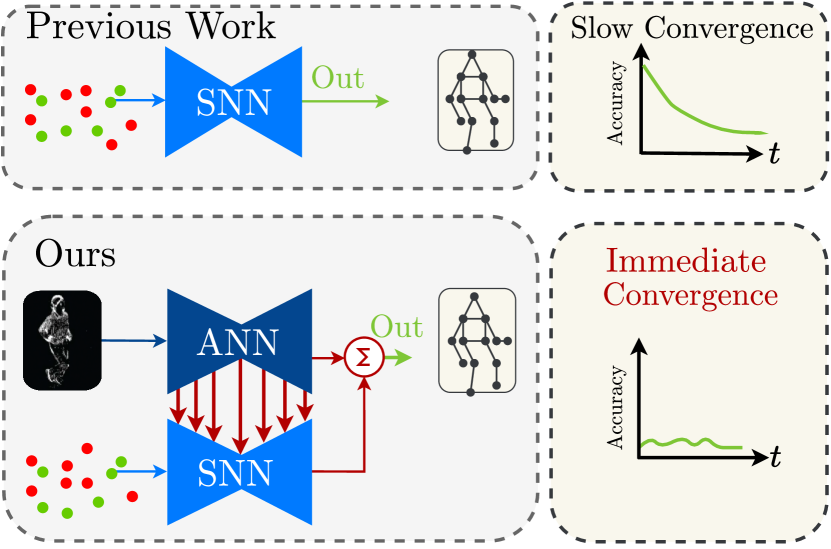
Figure 1: Spiking Neural Networks (SNNs, top) are prone to long transient periods and state decay in the absence of input data, leading to lower accuracy and higher latency and power consumption. In this work (bottom), we solve this with an auxiliary artificial neural network (ANN) that initializes the SNN states at low rates. Our resulting hybrid architecture is simultaneously accurate and maintains the low-power and low-latency aspect of SNNs.

Recent breakthroughs in deep learning have led to accelerating progress on a wide range of computer vision tasks. As this progress speed-ups, practitioners are moving to deeper and deeper models in the pursuit of higher task performance. However, this trend comes at a cost: Today’s large-scale models require increasing amounts of power, which limits their adoption in power-constrained scenarios.

Low-power computation is a crucial requirement for applications running on edge devices and can make the difference between changing the battery of IoT devices once a day or once a year or greatly increasing the mission time of autonomous robots with power-constrained hardware.

Spiking Neural Networks (SNNs) are a novel brain-inspired way to process visual signals, which are orders of magnitude more efficient than their Artificial Neural Network (ANN) counterparts. Instead of processing inputs as synchronous, analog-valued tensor maps, they are dynamical systems that process data as sparse spike trains. Moreover, when deployed on neuromorphic processors, SNNs function asynchronously in an activity-driven fashion, enabling fast inference and low power consumption.

Although previous work has demonstrated SNN applications on a wide range of tasks, they are still limited in their performance due to two shortcomings: First, they are difficult to train due to the non-differentiability of spikes [35] and the vanishing-gradient problem [39, 36]. Second, they require long time windows to converge and match the accuracy of ANNs [27, 10] and are prone to decay in the absence of input data. This is because SNNs, being temporal models, depend on an expressive state to generate predictions on par with classical ANNs. However, this state takes time to converge: Membrane potentials (i.e., states) in the SNN layers need to charge over time, then cross the firing threshold, and finally emit spikes that charge the next layer. In deep SNNs, this charging time generates a long delay, which increases latency and energy consumption due to the need for more iterations.

In this work, we solve this issue by using an auxiliary ANN to initialize the SNN states periodically at low rates, thus eliminating the need for the SNN states to converge. We then use the SNN to generate predictions and propagate the state forward until the next initialization step. The resulting predictions (i) have a high rate, (ii) experience a boost in accuracy due to a well-initialized state, and (iii) maintain the low-power property of SNNs. Crucially, the auxiliary ANN only requires little power due to the low rate of state initialization. The resulting hybrid model thus combines the advantages of both ANNs and SNNs.

We extensively evaluate our method on the tasks of 2D and 3D human pose estimation (HPE) using events from an event camera, where we show consistently that our method reduces the power consumption of standard ANNs by 88% while only achieving a 4% error increase. Instead, when compared to SNNs, our method achieves a 74% lower error.

1. We propose an energy-efficient, low-latency hybrid ANN-SNN architecture, where the ANN is tasked with initializing the SNN states at low frequency, thus overcoming the limitations of both ANNs and SNNs.

2. We show for the task of event-based HPE that this method achieves a balance between being accurate and power efficient. Compared to standard ANNs, it achieves significant improvements in terms of energy consumption and update rate while only experiencing a slight decrease in accuracy.

3. Finally, we show that our method outperforms pure SNN-based HPE algorithms by 74% in terms of accuracy while being 88% more energy efficient than ANN-based methods with only 4% higher error. This opens the door to robust, low-power, and low-latency human pose estimation.

2 Related work

2.1 Hybrid ANN-SNN Architectures

In recent years, there has been a growing interest in exploring the potential benefits of combining Artificial Neural Networks (ANNs) and Spiking Neural Networks (SNNs) [49, 25, 23, 28, 51]. Different combination strategies have been explored for a variety of tasks.

A group of work employs the strategy of processing the accumulated spike train of SNNs with ANNs [23, 28, 25]. In these works, the SNN is used as an efficient encoder of spatio-temporal event data from an event camera. The output of the SNN is accumulated to summarize the temporal dimension before the ANN processes the accumulated features [23, 25]. Liu et al. [28] extend this idea for object classification and use a feedback loop from the ANN to the input to the SNN. The downside of the aforementioned approaches is that they need to execute a full forward pass of the ANN to extract results, which results in high power consumption and high computational latency. In contrast, our SNN directly updates the output of the ANN such that we do not need to execute the ANN for every iteration, thus retaining the low-power property.

A second line of work uses a strategy where the output of the independently operating SNN and ANN is fused [26, 49, 51]. This approach is especially suitable for multimodal processing of frame-based video and event data from event cameras. The ANN is tasked with extracting features from the frames while the SNN processes events directly. Finally, the output of both networks are fused based on heuristics [26], temporal filtering [49], or accumulation based on the output of the ANN [51]. However, these methods do not address the convergence of SNN’s and also do not share features between networks, making their fusion shallow. By contrast, our approach not only reuses the output of the ANN [51] but also reuses the features from the ANN to initialize the SNN states. The initialization of SNN states drastically improves the performance and convergence of the SNN.

2.2 Human Pose Estimation

Frame-based

human pose estimation (HPE) is the task of estimating the 2D or 3D locations of body joints from a single image or video. Current techniques for 3D HPE involve reconstructing the 3D pose from either single [6, 33, 38, 46, 52, 7] or multiple [22, 15, 8, 41] camera views. To estimate the 3D pose from multiple views, the traditional approach involves predicting the 2D pose in each view and using the camera characteristics and positions to triangulate it into the world coordinate [1]. Alternatively, newer approaches include triangulation with neural networks [17, 29, 30, 20] or direct regression of the 3D pose [50, 41]. Both single-view and multi-view approaches can be improved by using multiple frames to extract temporal information that can help disambiguate joint locations over time and reduce jitters [34, 15, 8, 41, 20].

Recently, human pose estimation with event cameras has gained traction due to their inherent ability to filter out temporally redundant information like the background [48, 54, 3, 2, 44]. These works adopt one of two main approaches. The first direction of work utilizes volumetric human body models [31] to estimate both the 3D pose and shape of the human body [48, 54]. EventCap [48] and EventHPE [54] use a low-dimensional human shape representation called SMPL [31] to enable end-to-end shape and pose estimation from images and events. The second approach, in contrast, focuses on extracting the pose information using a skeleton body model [44, 3, 2]. Scarpellini et al. [44] use events from a single camera view and predict the 3D pose with a Convolutional Neural Network (CNN). Calabrese et al. [3] and Baldwin et al. [2] estimate 2D joint locations using a CNN architecture and perform triangulation to obtain the 3D pose. Different from previous work, we target low-power inference for human pose estimation using a hybrid ANN-SNN architecture. Our approach benefits from the high accuracy of ANNs and low power consumption of SNNs to improve the accuracy to power consumption tradeoff.

3 Methodology

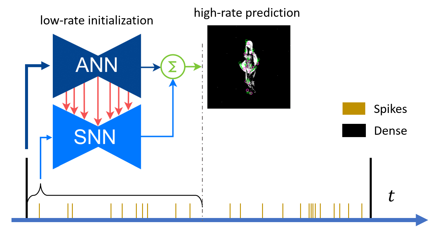
Figure 2: Overview of our method. Our method processes inputs as dense and spike-based representations. The ANN uses the dense representation to perform state and output initialization at low rates. The SNN then uses spikes to generate high-rate outputs until the next dense input.

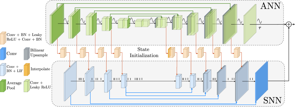
Figure 3: Hybrid ANN - SNN architecture. The ANN (upper row of blocks) is fed with past events at time step $t_{0}$, where an initial output is predicted, and states of spiking neurons are initialized (orange blocks). Events of duration $\Delta T$ are fed sequentially to the SNN (lower row of blocks), for high-rate updates of the prediction.

An overview of our approach is depicted in Fig. 2. In our hybrid ANN-SNN approach, the ANN is utilized to accurately predict joint locations based on prior events and to simultaneously initialize the spiking neuron states. This sets the stage for high-frequency, low-latency updates using the SNN, where events of duration $\Delta T$ are sequentially fed to the SNN. After the sequence duration $T$, the process is repeated where a new prediction is made by the ANN, and states of spiking neurons are re-initialized. The integration of the ANN at low rates and the SNN at high rates enables precise predictions to be made with low-latency while maintaining energy efficiency. The following sections provide a detailed explanation of our hybrid model and its constituent steps.

3.1 Preliminaries

Our method takes as input a sequence of spike-based and dense representations. The dense representation can be an image, if synchronized and aligned with events, or any dense event representation computed from raw events. For the remainder of this section, we let $Y_{i}$ be the dense representation at time $t_{i}$. In this work, we opted for stacked 2D histograms [12] in case of event data. They are computed by stacking $N=10$ two-channel histograms [32] from a total of 7,500 events. We then consider raw binary events up to time $t$ denoted as $X(t)$ with $t>t_{i}$:

$$X(t)=\sum_{j|t_{j}<t}p_{j}\delta(t-t_{j}).$$ (1)

In general, $t_{j}$ is the timestamp of the $j$-th events, and $p_{j}\in\mathbb{R}^{2}$ is the event polarity converted to a one-hot vector. The ANN, $F_{\text{ANN}}$, processes the dense event representation and predicts both the output $o$ at time $t$ as well as the initial SNN states $\{s^{k}\}_{k=1}^{L}$ for all $L$ layers. The SNN, $F_{\text{SNN}}$, then processes the incoming event stream $X$ to continuously update the prediction $o$. The following equations summarize this process:

$$\{s^{k}_{i}\}_{k=1}^{L},o_{i} =F_{\text{ANN}}(Y_{i})$$ (2)

$$o(t) =F_{\text{SNN}}(t;X,\{s^{k}_{i}\}_{k=1}^{L},o_{i}).$$ (3)

Here, $\{s^{k}_{i}\}_{k=1}^{L}$ denote the membrane potential of the SNNs at layers $k=1,...,L$ for timestamp $t_{i}$. The variable $o_{i}$ denotes the output map for timestamp $t_{i}$. Finally, $o(t)$ denotes the human pose estimates at time $t$ represented as 13 heatmaps, one for each body joint. The value at each pixel of the heatmap indicates the probability of finding the joint at that position. It is generated by using the initialization $o_{i}$ and integrating the output of the SNN onto it. In summary, the task of the SNN is to incrementally update the initial prediction that the ANN provides. While the ANN is a standard U-Net [42], the SNN can be interpreted as a continuous-time model that takes a function $X$ (see Eq. (1)) as input and generates a prediction at any time $t$. Next, we will go into more detail on how this model works.

3.2 Spiking Neural Network

SNNs model individual neurons at layer $k$ as dynamical systems that update their membrane potential $V^{k}$ by integrating a series of input spikes in a learnable way. When their membrane potential exceeds a threshold, it generates spikes which are then transmitted to the next layer, followed by some resetting of the membrane potential. In our work, we use the Leaky Integrate & Fire (LIF) neuron model [13]. The sub-threshold dynamics of a LIF neuron are defined as.

$$\tau\frac{dV^{k}(t)}{dt}=-(V^{k}(t)-V_{rest})+X^{k}(t).$$ (4)

Here $V^{k}(t)$ represents the neuron’s membrane potential at time t, and layer $k$, $V_{rest}$ is the resting potential of the neuron, $X^{k}(t)$ denotes the integrated spike train at time t, and $\tau$ is the membrane time constant. After the membrane potential reaches the firing threshold $V_{th}$, a spike is emitted, and the membrane potential is immediately reset back to its resting potential.

While conventionally, membrane potentials are initialized at 0 for all neurons and layers; we use the ANN to initialize these potentials in this work. We thus modify Eq. 4 by adding a boundary condition at time $t_{i}$ for each layer:

$$\tau\frac{dV^{k}(t)}{dt} =-(V^{k}(t)-V_{rest})+X^{k}(t).$$ (5)

$$\text{subj. to: }V^{k}(t_{i}) =s^{k}_{i}$$

where $s^{k}_{i}$ are the activation initialization maps generated by the ANN. As will be shown later, this small change has a major impact on the SNN behavior since it mitigates delays due to convergence in Eq. 4 and improves performance overall by providing a well-initialized state. Next, we will discuss how we emulate such a continuous dynamical system on conventional hardware.

3.3 Discretization and Training

To train our ANN-SNN model, we need to convert the SNN into a recurrent network. This is typically done by applying a forward Euler approximation to the differential Eq. (5). Eq. (6) shows the discretized sub-threshold dynamics, and the spiking mechanism where $H(.)$ is the Heaviside step function and $S_{t}$ denotes the spike output.

$$\begin{split}&V^{k}_{t}=V^{k}_{t-1}+\frac{1}{\tau}(X^{k}_{t}-(V^{k}_{t-1}-V_{rest}))\\ &S^{k}_{t}=H(V^{k}_{t}-V_{th})\\ \text{subj. to: }&V^{k}_{0}=s^{k}_{i}\end{split}$$ (6)

In the discretized version, time $t$ takes integer values and starts at index 0, which previously corresponded to the timestamp $t_{i}$. To emulate the resetting behavior, we apply soft resets, which reduce the potential by the amount of the threshold value. This allows the residual potential to be re-used at the next steps, resulting in reduced information loss. Using soft reset neurons has the effect that potential values can be initialized outside the range $[V_{rest},V_{thr}]$. This allows extreme cases such as dead neurons or always ON neurons. Soft reset neurons are also known as ”Residual Membrane Potential Neurons” [14].

Eqs. (6) can be interpreted as a recurrent neural network that can be unrolled over multiple forward Euler steps and then trained using backpropagation through time [47]. However, a challenge in training the above spiking neural networks lies in its use of the Heaviside step function $H$, which is not differentiable. However, this problem can be addressed by using surrogate gradients [35], i.e., replacing the gradient of the Heaviside function with the approximate

$$H^{\prime}(x)\approx\frac{1}{1+(\pi x)^{2}}$$ (7)

For more details on SNN training, see [35].

3.4 Network Details

The hybrid network details are illustrated in Fig. 3. For the ANN (top row), we use a U-Net structure [43], adapted from Super SloMo [18]. It has a total of 23 layers, comprising a prediction layer, five encoders, and five decoders concatenated with skip connections at the same spatial resolution. The SNN (bottom row) is a variant of the U-Net architecture [43], modified from EVSNN [53]. The architecture consists of 10 layers made up of a prediction layer, residual block, four encoder, and four decoder layers. At every timestep, events are presented to the network in two channels for each polarity. The network is trained with a discretization step of 10 ms. At the output, we use a simple convolutional layer and integrator, which allows predicting analog heatmaps. Each SNN layer is initialized from ANN state initialization modules depicted with orange blocks in Fig. 3. The initialization module reuses the ANN U-Net features and predicts the membrane potential of the SNN spiking neurons. The initialization modules consist of only two convolutional layers followed by batch normalization. An ablation study of the state initialization architectures can be found in Sec. 4.2.2. Additional network details about the ANN and SNN are given in the appendix.

4 Experiments

We evaluate our model on two publicly available event-based human pose estimation datasets, DHP19 [3] and Event-Human3.6M [44]. Sec. 4.1 starts off with details about the datasets, metrics, and training. We then demonstrate the effectiveness of our hybrid model in reducing power consumption while boosting accuracy in the ablation study section (Sec. 4.2). We conclude with a spike activity analysis in Sec. 4.3 and comparison with state-of-the-art event-based human pose estimators in Sec. 4.4.

4.1 Setup

Datasets

The DHP19 dataset [3] is a real-world event camera dataset recorded with 4 synchronized DAVIS346 cameras. Overall, the dataset features 17 different subjects performing a total of 33 movement patterns. DHP19 consists of 556 sequences with labels from a motion capture system at 100 Hz. With this dataset, we analyze our pure event-based implementation using real event data.

The Event-Human3.6M [44] originates from the Human3.6M dataset [16] and uses an event simulator [11] to generate synthetic event data. The dataset features 11 subjects and 17 different activities that are more complex than the movements in the DHP19 dataset. Human3.6M images are captured with 4 synchronized high-resolution cameras and labels with a motion capture system at 50 Hz. Our experiments on Event-Human3.6M examine whether our approach also performs well on more complex motion patterns at the cost of using synthetic event data.

Metrics

We measure the accuracy using the Mean Per Joint Position Error (MPJPE). For each joint, the Euclidean distance between the predicted and ground truth positions of a joint is calculated. The MPJPE score is computed as the mean of these errors across all joints in the skeleton body model. This score is defined for both 2D skeleton estimations (in pixels) and 3D estimation (in millimeters) as:

$$\centering\text{MPJPE}=\frac{1}{J}\sum_{i=1}^{J}\|{x_{i}-\hat{x}_{i}}\|,\@add@centering$$ (8)

where $J$ is the number of joints, $x_{i}$ is the ground truth, and $\hat{x}_{i}$ is the estimation of the joint in 2D or 3D space.

Energy Consumption

To measure energy consumption, we compute the total number of multiply-accumulate (MAC) and accumulate (AC) operations used by a method. While ANNs perform dense MAC operations, SNNs perform sparse AC operations as a result of the binary nature of spikes. In most technologies, the addition operation is less costly than the multiplication operation. For 7nm CMOS technology, one 32-bit MAC operation uses 1.69 pJ, while one AC only uses 0.38 pJ [19], which are the values we use to calculate the power consumption of all methods. For ANNs, we compute the total number of MACs throughout the layers as $k^{2}W_{o}W_{o}C_{i}C_{o}$, where we use the kernel size $k$, output dimension $W_{o}\times H_{o}$ and input and output channel dimension $C_{i}$ and $C_{o}$. For SNNs, we count the total number of ACs as the above value multiplied by the average spiking activity $\zeta^{l}\in[0,1]$. It is the ratio of the total number of spikes in layer $l$ over all timesteps to the total number of neurons in layer $l$ [40, 45, 24]. In these calculations, we assume every spike consumes constant energy [5].

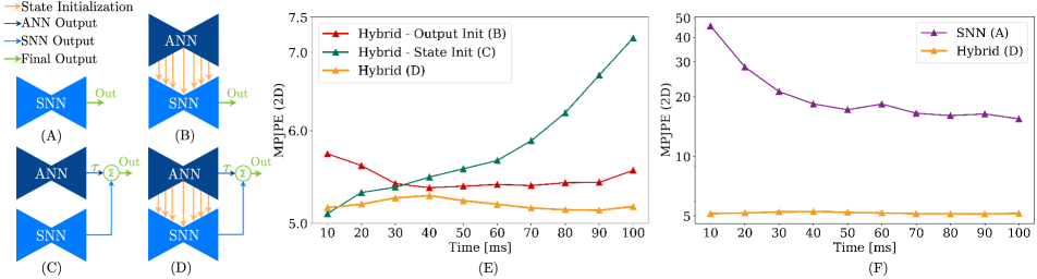
Figure 4: Overview of the ablation experiments. Schematic of (A) pure SNN without state initialization and output initialization, (B) hybrid model without output initialization, (C) hybrid model without state initialization, and (D) our proposed hybrid model with state and output initialization. Plots of accuracy over time of our approach against (E) only output initialization and only state initialization ablated and (F) both ablated. All plots provide 2D MPJPE scores on the entire test set for camera view #2.

Training Details

For SNN training, we use the Spiking Jelly framework [9], an open-source deep learning framework based on PyTorch [37]. The network is unrolled for all time steps to perform BPTT [47] on the average loss of the sequence, $L_{\text{avg}}$. We adopt the loss function from [4], which computes the difference between heatmaps generated by our method and labels generated from 3D joint labels projected to the pixel space. For each 2D joint, ground-truth heatmaps are generated by creating a 2D tensor of zeros at the same spatial resolution as the input with the joint location pixel set to 1. To facilitate learning, Gaussian blurring is applied with a filter size of 11 and a standard deviation of 2 pixels to each heatmap. The loss is computed with respect to the predicted and ground truth heatmaps using the Mean Square Error (MSE) and averaged over several timesteps

$$\centering L_{\text{avg}}=\frac{1}{JT}\sum_{t=1}^{T}\sum_{i=1}^{J}({o_{ti}-\hat{o}_{ti}})^{2},\@add@centering$$ (9)

All experiments were trained on a single GPU, Quadro RTX 8000, for approximately 72 hours. We first train an ANN with the learning rate 1e-4 of batch size 8 for 60,000 iterations. We then train the hybrid model by freezing the ANN weights and only training the SNN. Hybrid experiments were trained for 280,000 iterations with an Adam optimizer [21], batch size 2, and learning rate 5e-5 with the neuronal time constant, firing threshold, and output decay $\tau$ set to 3, 1, and 0.8, respectively. Pure SNN experiments were trained for 160,000 iterations with the same parameters, with the exception of the time constant $\tau=2$.

Table 1: State initialization module ablation study on the validation set. Results are reported on the camera view #2. The last bin provides the score of the $10^{th}$ time step, and the second column reports the average score of the sequence.

State Initialization Mappings	MPJPE (2D) $\downarrow$
	Last Bin	Average
-	9.12	7.08
Conv + BN + LeakyReLU + Conv + BN + Sigmoid	16.59	9.83
Conv + BN + LeakyReLU + Conv + BN + LeakyReLU	6.32	6.14
Conv + BN + LeakyReLU + Conv + BN	6.11	6.02
Conv + BN + LeakyReLU + Conv	6.22	6.23
Conv + BN + LeakyReLU	6.12	6.17

4.2 Ablation Studies

This section first examines the two main contributors to the performance of our proposed model, state initialization and output initialization. Second, we examine different state initialization architectures.

4.2.1 Proposed Method

Fig. 4 reports ablation studies comparing four variants of our method (A-D) in terms of 2D MPJPE on camera view 2 of DHP19. In E-F, we show the MPJPE over 100 ms of events. Model A is a pure SNN with a zero state initialization at time 0. Model B initializes the SNN states from an auxiliary ANN. This ANN processes a dense event representation constructed at time $t=0$ to generate these states, and the SNN then continues predicting within the time interval. Model C does not use state initialization but instead uses the SNN to learn a delta on the ANN prediction at timestamp $t=0$, which we call output initialization. Finally, model D combines the idea of output initialization and state initialization, which is our proposed method.

We see in Fig. 4 (F) that the SNN (A), initialized at 0, achieves a high error due to a slow convergence over the time interval shown. One way to solve this is to use output initialization, which achieves a low error at the beginning (E) but diverges back to pure-SNN error levels the further away we get from the first ANN prediction. Our proposed way to initialize SNN states via the ANN (B) accelerates the convergence of the SNN and thus leads to stable and low error rates in (E). Finally, adding back output initialization further reduces the error rate consistently throughout the interval. Crucially, using output initialization upper bounds the method’s error rate at $t=0$ to that of the ANN.

4.2.2 State Initialization Architecture

We investigate different blocks for mapping ANN features to initialize membrane potentials (Fig. 3, orange blocks) and report the last bin and average bin scores in Tab. 1. For the last bin, we report the error achieved after 100 ms of events, and for the average bin score, we average over 10 time steps.

We compare these scores with membrane potentials initialized with zeros reported in the first row. In general, we found that putting a batch normalization layer at the end led to the best results. Interestingly, since batch normalization can generate values outside of the range [0,1], it can permanently kill or activate neurons which proved to be beneficial. This can be seen when comparing rows 2 to 4, where adding a range limiting function LeakyReLU or Sigmoid degrades performance. Following Tab. 1, we chose Conv + BN + LeakyReLU + Conv + BN.

4.3 Spike Activity Analysis

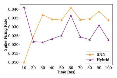
Figure 5: Effect of state initialization on spike firing rates across time steps. The SNN before state initialization consumes 46 mW of energy, while after state initialization, this decreases to 30 mW.

This section compares spike activity before and after state initialization of spiking neurons. Fig. 5 shows the average spike firing rate throughout the network for each time step. The spike rate gradually increases for the SNN experiment as membrane potentials build up and more spikes are emitted over time. In contrast, spike firing rates in the hybrid model show high firing rates in the first time step due to the initialized states. Overall, there is reduced firing activity following state initialization, leading to a 35% decrease in power consumption from 46 mW to 30 mW.

4.4 Comparison with State-of-the-Art

4.4.1 2D Pose Estimation

Here we compare the performance of our approach and its ANN counterpart with previous work on 2D pose estimation. ANN experiments reported at a specific rate are achieved by inputting events in a sliding window manner. Tab. 2 reports 2D results on the test set for DHP19 [3] and compares MPJPE in pixels on the two camera views used in prior work. We compare against Calabrese et al. [4], which uses an Hourglass style network to process dense event representations, and Baldwin et al. [2], which reuses the network from [4] but instead uses specialized TORE volumes as inputs. Both methods use artificial neural networks.

Tab. 2 shows that our pure ANN achieves the best score with 5.03 px compared to all previous methods but consumes the most energy with 3.718 W. In contrast, the hybrid model with 0.424 W is 8x more energy efficient compared to the pure ANN model, with only a 6% and 3% decrease in accuracy for camera views 3 and 2, respectively. In comparison with previous work, the hybrid model is the most energy efficient while outperforming previous works. A key advantage of using SNNs is that outputs are continuous time, meaning that we may increase the discretization step of the SNN to smaller values, i.e., higher rate outputs, without significantly impacting power consumption. Fig. 6 visualizes all methods’ accuracy and power consumption at different rates. The SNN part of our hybrid model only consumes %5 of the energy. Therefore, increasing the update rate allows higher rate predictions with little to no increase in power consumption while maintaining the same accuracy. For approaches relying only on ANNs, power consumption increases linearly with the prediction rate. From Fig. 6, we see that our hybrid model at 200 Hz retains good accuracy with minimal change in power consumption. Fig. 7 visualizes the tracking performance of our approach at 100 Hz for different movements and test subjects, in comparison to ANN at 10 and 100 Hz.

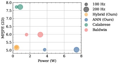
Figure 6: 2D pose estimation performance vs. power consumption at 100 and 200 Hz.

Table 2: 2D pose estimation performance on DHP19 at 100 Hz together with energy consumption results. Best values are highlighted in bold, and second best are underlined.

Method	Model	2D MPJPE $\downarrow$		# Ops/s (G)		Power (W)
		Cam 2	Cam 3	MAC	AC
Calabrese [3]	ANN	7.72	7.61	255	0	0.431
Baldwin [2]	ANN	5.98	5.25	949	0	1.605
Ours	ANN	5.03	4.67	2200	0	3.718
Ours	SNN	21.37	19.17	0.5	121	0.046
Ours	Hybrid	5.19	4.97	233	79	0.424

Next, we evaluate our approach on the Event-Human3.6M [44] dataset. We perform two experiments, feeding either RGB images or event representation to the ANN. This shows our approach’s generality to work with multimodal (events+frames) data. The ANN is deployed at 5 Hz, while the SNN uses a discretization step of 10 ms, resulting in 100 Hz updates. Tab. 3 reports our scores and power consumption. Our hybrid approach with RGB images fed to the ANN reports on par accuracy of 4.66 pixels with previous work while being 26.7 times more energy efficient with 0.21 W power consumption compared to the 5.61 W of previous work. Due to the model complexity of previous work, our hybrid experiments with only events, the last row of Tab. 3, fall short of state-of-the-art but show competitive performance.

Table 3: 2D pose estimation score on Event-Human3.6M at 100 Hz together with energy consumption results.

Method	Model	Modality	2D MPJPE $\downarrow$	# Ops/s (G)		Power (W)
				MAC	AC
Scarpellini [44]	ANN	Events	4.66	3321	0	5.61
Ours	ANN	RGB	4.19	2025	0	3.42
Ours	ANN	Events	5.09	2200	0	3.72
Ours	Hybrid	RGB + Events	4.66	108	75	0.21
Ours	Hybrid	Events	5.76	117	70	0.22

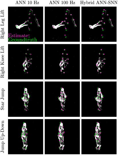
Figure 7: Qualitative 2D pose estimation results for different test subjects and movements. From left to right, samples from ANN at 10 Hz, 100 Hz, and our hybrid ANN - SNN model at 100 Hz with green markers indicating groundtruth and pink markers indicating predictions. Large circles indicate the end prediction of the sequence.

Table 4: 3D pose estimation scores on DHP19. MPJPE is reported in millimeters.

Method	Model	Triang.	3D MPJPE $\downarrow$	# Ops/s (G)		Power (W)
				MAC	AC
Calabrese [3]	ANN	Geom.	87.6	255	0	0.431
Baldwin [2]	ANN	NN	58.4	984	0	1.664
Ours	Hybrid	Geom.	57.7	233	79	0.424
Ours	Hybrid	NN	54.2	268	79	0.483

4.4.2 3D Pose Estimation

For 3D HPE on the DHP19 dataset, we use the 2D detection provided by our method and then use two triangulation methods to generate 3D points: First, we use geometrical triangulation from the two camera views to compare against Calabrese et al. [3]. Second, we use neural network-based (learned) triangulation for a fair comparison with Baldwin et al. [2]. Tab. 4 summarizes the results and shows that our approach yields the best trade-off between performance and energy consumption. Our hybrid approach with geometrical triangulation requires less power than Calabrese et al. [3] while substantially reducing the MPJPE by 34%, from 87.6 mm to 57.7 mm. When using learned triangulation, our method achieves an MPJPE reduction of 4.2 mm compared to Baldwin et al. [2], previous state-of-the-art, while at the same time consuming 3.4 times less energy.

5 Conclusion

We presented a hybrid ANN-SNN architecture that delivers fast and precise inference with reduced computational costs. Our work identified that the slow convergence of SNNs is due to the initialization of spiking neuron membrane states. Our solution to this problem involves initializing both SNN states and the output state with an ANN. This approach enables SNNs to immediately produce accurate predictions without requiring a warm-up phase, thereby reducing latency. Our experimental results demonstrate that this hybrid architecture can reduce energy consumption up to 88%, with only a 4% decrease in performance on human pose estimation with respect to a standard ANN. When compared to SNNs, our method achieves a 74% lower error. We anticipate that this research will inspire further investigations at the intersection of neuromorphic engineering and conventional deep learning.

6 Acknowledgement

This work was supported by the National Centre of Competence in Research (NCCR) Robotics (grant agreement No. 51NF40-185543) through the Swiss National Science Foundation (SNSF), and the European Research Council (ERC) under grant agreement No. 864042 (AGILEFLIGHT).

7 Appendix

7.1 Overview

Here, we provide additional information supporting the main manuscript. In what follows we will refer to Figures, Tables, Sections, and Equations from the main manuscript with the prefix “M-”, and use no prefix for new references in the appendix. We start by providing further analysis of our state initialization scheme (Sec. 7.2), then provide additional network details in Sec. 7.3. We, also attach a supplementary video with visualizations of our low-latency human pose estimation network’s output.

7.2 Initialized Membrane Potential Values

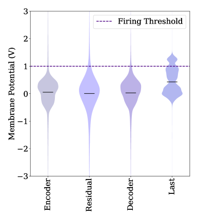
Figure 8: Violin plots of membrane potential values after state initialization across layers of the SNN. Black lines indicate the mean state value at every layer. ‘Last’ indicates the last state initialized layer before the output.

In Fig. 8 we show the distribution of initial membrane potentials predicted by our ANN, grouped by the encoder, residual blocks, decoder, and last initialized layer before the output. Note that the firing threshold is 1, meaning that certain neurons are initialized in a firing state. In particular, the output layer shows a high proportion of these kinds of neurons. We call these states that are initialized close to firing, or even in a firing state meta-stable. This meta-stable state is important to reduce latency since it means that few input events can immediately elicit a network response since the membrane potentials are close to firing. We also see a long tail of inhibited neurons that are initialized with a negative membrane potential.

7.3 Network Details

The CNN and SNN architecture details are given in Tables 5 and 6, respectively. For each layer, padding is calculated to preserve spatial dimensions. Both tables are given with respect to the resolution of the DHP19 dataset, 256x256. For the Event-Human3.6M dataset, the resolution is 320x256.

Each convolutional layer in the CNN is followed by a leaky ReLU layer with a negative slope of 0.1. Columns 1-6, are the encoder layers where an average pooling layer is followed by two convolutions. Columns 7-11 are decoder layers, and operations are as follows: (i) interpolation, (ii) convolutional layer, (iii) concatenation with skip connections of the same resolution, and (iv) convolution. Finally, the last column is a simple prediction layer with no activation function.

Each convolutional layer in the SNN is followed by a batch norm, and leaky integrate & fire neuron layer. The first column is the spike encoder, columns 2-4 are encoder, 5-6 are residual, and 7-9 are decoder layers. Decoder blocks perform concatenation with skip connections at the same spatial resolution and are upsampled together. Finally, the last layer is a single convolutional layer.

Table 5: CNN architecture details. Changes in spatial resolution are due to 2x2 average pooling or bilinear interpolation by a scale of 2. The input channel is of size 20 for event representations or 3 for RGB images.

Layer	1	2	3	4	5	6	7	8	9	10	11	12
Kernel size	7	5	3	3	3	3	3	3	3	3	3	3
Output channel	32	64	128	256	512	512	512	256	128	64	32	13
Output H, W	256	128	64	32	16	8	16	32	64	128	256	256

Table 6: SNN architecture details. Changes in spatial resolution are due to convolutions with stride 2 and bilinear interpolation of scale 2. The input channel is of size 2.

Layer	1	2	3	4	5	6	7	8	9	10
Kernel size	5	5	5	5	3	3	5	5	5	1
Stride	1	2	2	2	1	1	1	1	1	1
Output channel	32	64	128	256	256	256	128	64	32	13
Output H, W	256	128	64	32	32	32	64	128	256	256

References

- [1] Sikandar Amin, Mykhaylo Andriluka, Marcus Rohrbach, and Bernt Schiele. Multi-view pictorial structures for 3d human pose estimation. In British Mach. Vis. Conf. (BMVC), volume 1. Bristol, UK, 2013.
- [2] Raymond Baldwin, Ruixu Liu, Mohammed Mutlaq Almatrafi, Vijayan K Asari, and Keigo Hirakawa. Time-ordered recent event (tore) volumes for event cameras. IEEE Trans. Pattern Anal. Mach. Intell., 2022.
- [3] Enrico Calabrese, Gemma Taverni, Christopher Awai Easthope, Sophie Skriabine, Federico Corradi, Luca Longinotti, Kynan Eng, and Tobi Delbruck. Dhp19: Dynamic vision sensor 3d human pose dataset. In IEEE/CVF Conference on Computer Vision and Pattern Recognition Workshops (CVPRW), pages 1695–1704, 2019.
- [4] Enrico Calabrese, Gemma Taverni, Christopher Awai Easthope, Sophie Skriabine, Federico Corradi, Luca Longinotti, Kynan Eng, and Tobi Delbruck. DHP19: Dynamic vision sensor 3D human pose dataset. In IEEE Conf. Comput. Vis. Pattern Recog. Workshops (CVPRW), 2019.
- [5] Yongqiang Cao, Yang Chen, and Deepak Khosla. Spiking deep convolutional neural networks for energy-efficient object recognition. Int. J. Comput. Vis., 113(1):54–66, 2015.
- [6] Ching-Hang Chen and Deva Ramanan. 3d human pose estimation= 2d pose estimation+ matching. In IEEE Conf. Comput. Vis. Pattern Recog. (CVPR), pages 7035–7043, 2017.
- [7] Yucheng Chen, Yingli Tian, and Mingyi He. Monocular human pose estimation: A survey of deep learning-based methods. Computer Vision and Image Understanding, 192:102897, 2020.
- [8] Ahmed Elhayek, Edilson de Aguiar, Arjun Jain, Jonathan Tompson, Leonid Pishchulin, Micha Andriluka, Chris Bregler, Bernt Schiele, and Christian Theobalt. Efficient convnet-based marker-less motion capture in general scenes with a low number of cameras. In IEEE Conf. Comput. Vis. Pattern Recog. (CVPR), pages 3810–3818, 2015.
- [9] Wei Fang, Yanqi Chen, Jianhao Ding, Ding Chen, Zhaofei Yu, Huihui Zhou, Yonghong Tian, et al. Spikingjelly. https://github.com/fangwei123456/spikingjelly, 2020. Accessed: 2022-11-18.
- [10] Wei Fang, Zhaofei Yu, Yanqi Chen, Tiejun Huang, Timothée Masquelier, and Yonghong Tian. Deep residual learning in spiking neural networks. Conf. Neural Inf. Process. Syst. (NeurIPS), 34:21056–21069, 2021.
- [11] Daniel Gehrig, Mathias Gehrig, Javier Hidalgo-Carrió, and Davide Scaramuzza. Video to events: Recycling video datasets for event cameras. In IEEE Conf. Comput. Vis. Pattern Recog. (CVPR), June 2020.
- [12] Daniel Gehrig, Antonio Loquercio, Konstantinos G. Derpanis, and Davide Scaramuzza. End-to-end learning of representations for asynchronous event-based data. In Int. Conf. Comput. Vis. (ICCV), 2019.
- [13] Wulfram Gerstner, Werner M Kistler, Richard Naud, and Liam Paninski. Neuronal dynamics: From single neurons to networks and models of cognition. Cambridge University Press, 2014.
- [14] Bing Han, Gopalakrishnan Srinivasan, and Kaushik Roy. Rmp-snn: Residual membrane potential neuron for enabling deeper high-accuracy and low-latency spiking neural network. In IEEE Conf. Comput. Vis. Pattern Recog. (CVPR), pages 13558–13567, 2020.
- [15] Michael Hofmann and Dariu M Gavrila. Multi-view 3d human pose estimation in complex environment. Int. J. Comput. Vis., 96:103–124, 2012.
- [16] Catalin Ionescu, Dragos Papava, Vlad Olaru, and Cristian Sminchisescu. Human3.6m: Large scale datasets and predictive methods for 3d human sensing in natural environments. IEEE Trans. Pattern Anal. Mach. Intell., 36(7):1325–1339, 2014.
- [17] Karim Iskakov, Egor Burkov, Victor Lempitsky, and Yury Malkov. Learnable triangulation of human pose. In Int. Conf. Comput. Vis. (ICCV), 2019.
- [18] Huaizu Jiang, Deqing Sun, Varun Jampani, Ming-Hsuan Yang, Erik Learned-Miller, and Jan Kautz. Super slomo: High quality estimation of multiple intermediate frames for video interpolation. In IEEE Conf. Comput. Vis. Pattern Recog. (CVPR), pages 9000–9008, 2018.
- [19] Norman P. Jouppi, Doe Hyun Yoon, Matthew Ashcraft, Mark Gottscho, Thomas B. Jablin, George Kurian, James Laudon, Sheng Li, Peter Ma, Xiaoyu Ma, Thomas Norrie, Nishant Patil, Sushma Prasad, Cliff Young, Zongwei Zhou, and David Patterson. Ten lessons from three generations shaped google’s tpuv4i : Industrial product. In 2021 ACM/IEEE 48th Annual International Symposium on Computer Architecture (ISCA), pages 1–14, 2021.
- [20] Isinsu Katircioglu, Bugra Tekin, Mathieu Salzmann, Vincent Lepetit, and Pascal Fua. Learning latent representations of 3d human pose with deep neural networks. Int. J. Comput. Vis., 126:1326–1341, 2018.
- [21] Diederik P. Kingma and Jimmy L. Ba. Adam: A method for stochastic optimization. Int. Conf. Learn. Representations (ICLR), 2015.
- [22] Muhammed Kocabas, Salih Karagoz, and Emre Akbas. Self-supervised learning of 3d human pose using multi-view geometry. In IEEE Conf. Comput. Vis. Pattern Recog. (CVPR), pages 1077–1086, 2019.
- [23] Alexander Kugele, Thomas Pfeil, Michael Pfeiffer, and Elisabetta Chicca. Hybrid snn-ann: Energy-efficient classification and object detection for event-based vision. In DAGM German Conference on Pattern Recognition, 2021.
- [24] Souvik Kundu, Gourav Datta, Massoud Pedram, and Peter A Beerel. Spike-thrift: Towards energy-efficient deep spiking neural networks by limiting spiking activity via attention-guided compression. In IEEE Winter Conf. Appl. Comput. Vis. (WACV), pages 3953–3962, 2021.
- [25] Chankyu Lee, Adarsh Kumar Kosta, Alex Zihao Zhu, Kenneth Chaney, Kostas Daniilidis, and Kaushik Roy. Spike-flownet: event-based optical flow estimation with energy-efficient hybrid neural networks. In Eur. Conf. Comput. Vis. (ECCV), pages 366–382. Springer, 2020.
- [26] Ashwin Sanjay Lele, Yan Fang, Aqeel Anwar, and Arijit Raychowdhury. Bio-mimetic high-speed target localization with fused frame and event vision for edge application. Frontiers in Neuroscience, 16, 2022.
- [27] Yuhang Li, Shikuang Deng, Xin Dong, Ruihao Gong, and Shi Gu. A free lunch from ann: Towards efficient, accurate spiking neural networks calibration. In Proc. Int. Conf. Mach. Learning (ICML), pages 6316–6325. PMLR, 2021.
- [28] Faqiang Liu and Rong Zhao. Enhancing spiking neural networks with hybrid top-down attention. Frontiers in Neuroscience, 16, 2022.
- [29] Ruixu Liu, Ju Shen, He Wang, Chen Chen, Sen-ching Cheung, and Vijayan Asari. Attention mechanism exploits temporal contexts: Real-time 3d human pose reconstruction. In IEEE Conf. Comput. Vis. Pattern Recog. (CVPR), pages 5064–5073, 2020.
- [30] Ruixu Liu, Ju Shen, He Wang, Chen Chen, Sen-ching Cheung, and Vijayan K Asari. Enhanced 3d human pose estimation from videos by using attention-based neural network with dilated convolutions. Int. J. Comput. Vis., 129:1596–1615, 2021.
- [31] Matthew Loper, Naureen Mahmood, Javier Romero, Gerard Pons-Moll, and Michael J Black. Smpl: A skinned multi-person linear model. ACM transactions on graphics (TOG), 34(6):1–16, 2015.
- [32] Ana I. Maqueda, Antonio Loquercio, Guillermo Gallego, Narciso García, and Davide Scaramuzza. Event-based vision meets deep learning on steering prediction for self-driving cars. In IEEE Conf. Comput. Vis. Pattern Recog. (CVPR), pages 5419–5427, 2018.
- [33] Dushyant Mehta, Oleksandr Sotnychenko, Franziska Mueller, Weipeng Xu, Srinath Sridhar, Gerard Pons-Moll, and Christian Theobalt. Single-shot multi-person 3d pose estimation from monocular rgb. In 3D Vision (3DV), pages 120–130. IEEE, 2018.
- [34] Dushyant Mehta, Srinath Sridhar, Oleksandr Sotnychenko, Helge Rhodin, Mohammad Shafiei, Hans-Peter Seidel, Weipeng Xu, Dan Casas, and Christian Theobalt. Vnect: Real-time 3d human pose estimation with a single rgb camera. Acm transactions on graphics (tog), 36(4):1–14, 2017.
- [35] Emre O Neftci, Hesham Mostafa, and Friedemann Zenke. Surrogate gradient learning in spiking neural networks: Bringing the power of gradient-based optimization to spiking neural networks. IEEE Signal Processing Magazine, 36(6):51–63, 2019.
- [36] Razvan Pascanu, Tomas Mikolov, and Yoshua Bengio. On the difficulty of training recurrent neural networks. In Proc. Int. Conf. Mach. Learning (ICML), pages 1310–1318. PMLR, 2013.
- [37] Adam Paszke, Sam Gross, Francisco Massa, Adam Lerer, James Bradbury, Gregory Chanan, Trevor Killeen, Zeming Lin, Natalia Gimelshein, Luca Antiga, et al. Pytorch: An imperative style, high-performance deep learning library. Conf. Neural Inf. Process. Syst. (NeurIPS), 32, 2019.
- [38] Georgios Pavlakos, Xiaowei Zhou, Konstantinos G Derpanis, and Kostas Daniilidis. Coarse-to-fine volumetric prediction for single-image 3d human pose. In IEEE Conf. Comput. Vis. Pattern Recog. (CVPR), pages 7025–7034, 2017.
- [39] Wachirawit Ponghiran and Kaushik Roy. Spiking neural networks with improved inherent recurrence dynamics for sequential learning. In AAAI Conf. Artificial Intell., volume 36, pages 8001–8008, 2022.
- [40] Nitin Rathi, Gopalakrishnan Srinivasan, Priyadarshini Panda, and Kaushik Roy. Enabling deep spiking neural networks with hybrid conversion and spike timing dependent backpropagation. arXiv preprint arXiv:2005.01807, 2020.
- [41] Helge Rhodin, Nadia Robertini, Dan Casas, Christian Richardt, Hans-Peter Seidel, and Christian Theobalt. General automatic human shape and motion capture using volumetric contour cues. In Eur. Conf. Comput. Vis. (ECCV), pages 509–526. Springer, 2016.
- [42] Olaf Ronneberger, Philipp Fischer, and Thomas Brox. U-net: Convolutional networks for biomedical image segmentation. In International Conference on Medical Image Computing and Computer-Assisted Intervention, 2015.
- [43] Olaf Ronneberger, Philipp Fischer, and Thomas Brox. U-net: Convolutional networks for biomedical image segmentation. In International Conference on Medical Image Computing and Computer-Assisted Intervention, pages 234–241. Springer, 2015.
- [44] Gianluca Scarpellini, Pietro Morerio, and Alessio Del Bue. Lifting monocular events to 3d human poses. In IEEE Conf. Comput. Vis. Pattern Recog. (CVPR), pages 1358–1368, 2021.
- [45] Abhronil Sengupta, Yuting Ye, Robert Wang, Chiao Liu, and Kaushik Roy. Going deeper in spiking neural networks: Vgg and residual architectures. Frontiers in neuroscience, 13:95, 2019.
- [46] Denis Tome, Chris Russell, and Lourdes Agapito. Lifting from the deep: Convolutional 3d pose estimation from a single image. In IEEE Conf. Comput. Vis. Pattern Recog. (CVPR), pages 2500–2509, 2017.
- [47] P.J. Werbos. Backpropagation through time: what it does and how to do it. Proceedings of the IEEE, 78(10):1550–1560, 1990.
- [48] Lan Xu, Weipeng Xu, Vladislav Golyanik, Marc Habermann, Lu Fang, and Christian Theobalt. Eventcap: Monocular 3d capture of high-speed human motions using an event camera. In IEEE Conf. Comput. Vis. Pattern Recog. (CVPR), pages 4968–4978, 2020.
- [49] Zheyu Yang, Yujie Wu, Guanrui Wang, Yukuan Yang, Guoqi Li, Lei Deng, Jun Zhu, and Luping Shi. Dashnet: a hybrid artificial and spiking neural network for high-speed object tracking. arXiv preprint arXiv:1909.12942, 2019.
- [50] Pengfei Yao, Zheng Fang, Fan Wu, Yao Feng, and Jiwei Li. Densebody: Directly regressing dense 3d human pose and shape from a single color image. arXiv preprint arXiv:1903.10153, 2019.
- [51] Rong Zhao, Zheyu Yang, Hao Zheng, Yujie Wu, Faqiang Liu, Zhenzhi Wu, Lukai Li, Feng Chen, Seng Song, Jun Zhu, et al. A framework for the general design and computation of hybrid neural networks. Nature communications, 13(1):1–12, 2022.
- [52] Xingyi Zhou, Qixing Huang, Xiao Sun, Xiangyang Xue, and Yichen Wei. Towards 3d human pose estimation in the wild: a weakly-supervised approach. In IEEE Conf. Comput. Vis. Pattern Recog. (CVPR), pages 398–407, 2017.
- [53] Lin Zhu, Xiao Wang, Yi Chang, Jianing Li, Tiejun Huang, and Yonghong Tian. Event-based video reconstruction via potential-assisted spiking neural network. In IEEE Conf. Comput. Vis. Pattern Recog. (CVPR), pages 3594–3604, 2022.
- [54] Shihao Zou, Chuan Guo, Xinxin Zuo, Sen Wang, Pengyu Wang, Xiaoqin Hu, Shoushun Chen, Minglun Gong, and Li Cheng. Eventhpe: Event-based 3d human pose and shape estimation. In IEEE Conf. Comput. Vis. Pattern Recog. (CVPR), pages 10996–11005, 2021.