How many dimensions are required to find an adversarial example?

Abstract

Past work exploring adversarial vulnerability have focused on situations where an adversary can perturb all dimensions of model input. On the other hand, a range of recent works consider the case where either (i) an adversary can perturb a limited number of input parameters or (ii) a subset of modalities in a multimodal problem. In both of these cases, adversarial examples are effectively constrained to a subspace $V$ in the ambient input space $\mathcal{X}$. Motivated by this, in this work we investigate how adversarial vulnerability depends on $\dim(V)$. In particular, we show that the adversarial success of standard PGD attacks with $\ell^{p}$ norm constraints behaves like a monotonically increasing function of $\epsilon(\frac{\dim(V)}{\dim\mathcal{X}})^{\frac{1}{q}}$ where $\epsilon$ is the perturbation budget and $\frac{1}{p}+\frac{1}{q}=1$, provided $p>1$ (the case $p=1$ presents additional subtleties which we analyze in some detail). This functional form can be easily derived from a simple toy linear model, and as such our results land further credence to arguments that adversarial examples are endemic to locally linear models on high dimensional spaces.

1 Introduction

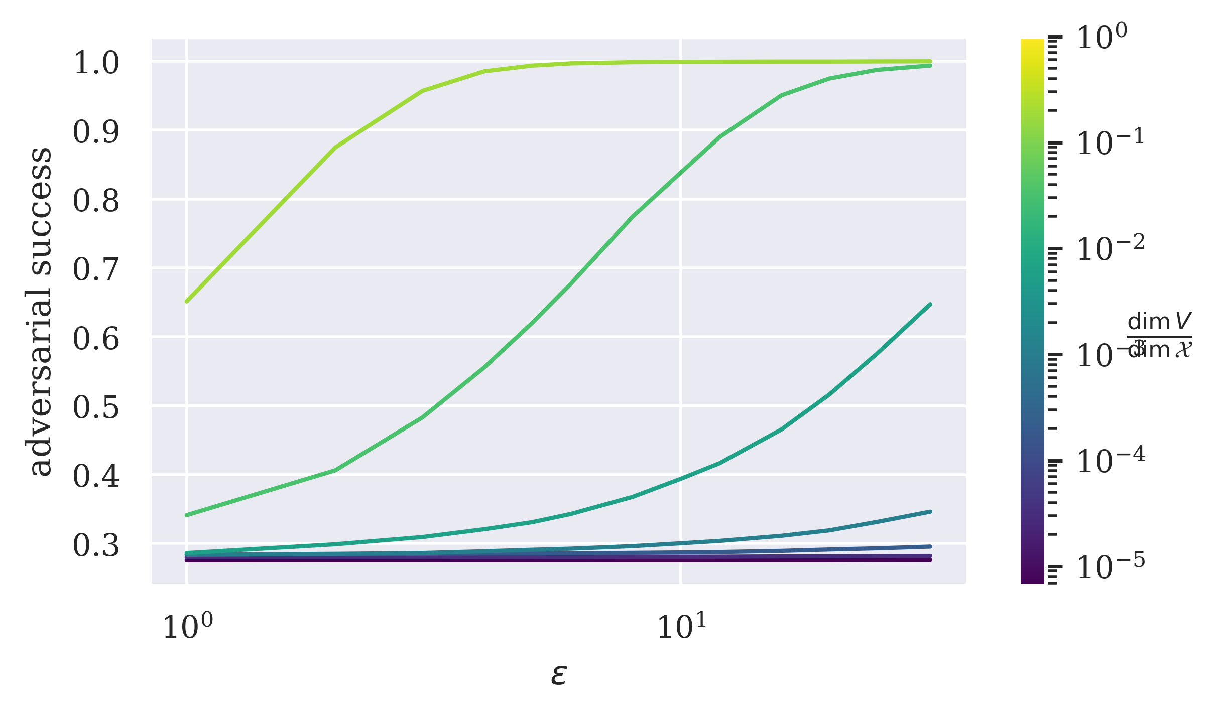
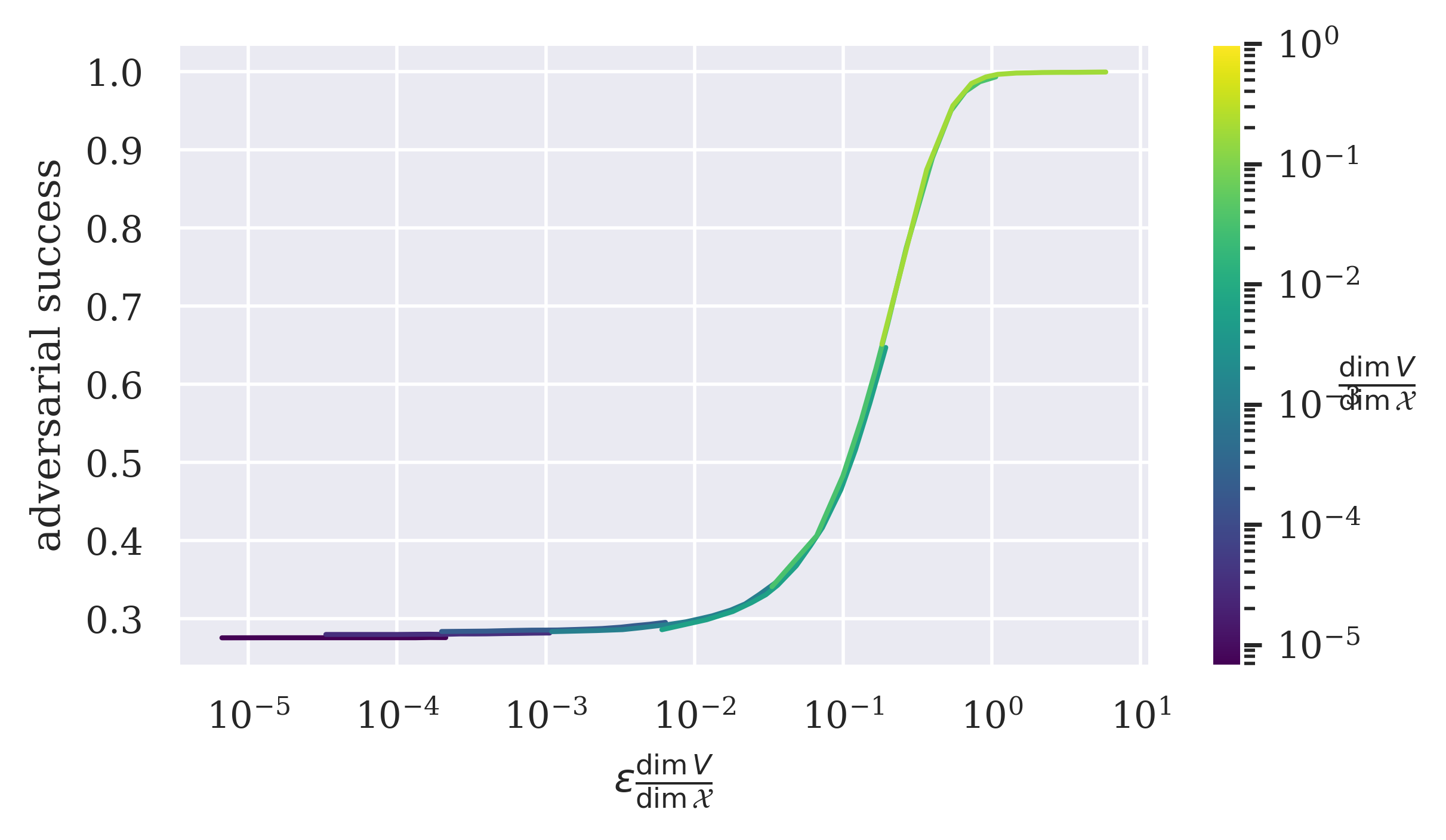
Figure 1: Left: success of PGD adversarial attacks on an ImageNet trained ResNet50, with $\ell^{\infty}$-norm constraints on perturbation budget, constrained to subspaces $V\subseteq\mathcal{X}$ spanned by $\dim V$ randomly selected standard basis vectors. Adversarial examples are computed for a random subsample of 10,000 datapoints from the ImageNet validations set. The $x$-axis is the $\epsilon$-bound used during example generation and the different colored curves indicate the dimension $\dim V$ of the subspace to which the examples were constrained to, relative to the dimension $\dim\mathcal{X}$ ($=3\cdot 224^{2}$) of the ambient space. When only a small number of dimensions can be perturbed, adversarial examples are challenging to generate even with large $\epsilon$-bounds. Right: these curves become aligned when we reparameterize the $x$-axis by scaling by $\frac{\dim V}{\dim\mathcal{X}}$.

Since they were first identified in [33], there has been strong sense that a model’s vulnerability to adversarial examples is strongly connected to the dimension of its input space. This connection has been mined by a range of works which use it as a perspective with which to explain the prevalence of adversarial examples in certain model types (e.g., computer vision) – in Sec. 2 we provide a brief synopsis of this research. As deep learning models are applied to more and more safety critical applications, there is also an increasing practical relevance to understanding any general connections between adversarial vulnerability and the properties of a problem. In such settings, a simple statistic that can be easily computed (such as model input dimension) is useful for gauging the general adversarial risk for a proposed deep learning system.

This is especially true when the proposed system uses less familiar modalities/tasks to which one cannot easily refer to studies in the literature. For example, suppose one needs to evaluate the safety of applying deep learning to the output of a range of different sensors. Past work has considered the ambient dimension in which this data is collected. Should we worry less if a sensor captures a signal as a $50$-dimensional vector rather than a $5,000$-dimensional vector? In this paper we take this line of reasoning a step further and ask how this situation changes when instead of changing the ambient dimension we change the dimension of the subspace in which one is constrained to perturb input. Such a thought experiment has practical relevance. Suppose that of the $500$ input dimensions to our model, we believe that an adversary is only likely to get access to $50$ dimensions (this may happen in multimodal settings where an adversary has much better access to a subset of the modalities). How should we compare this to a situation in which are only able to perturb a fixed $100$-dimensional subspace of the input? How about a $5$-dimensional subspace?

Motivated by this, in this work we revisit the connection between dimension and adversarial vulnerability. Unlike most other works in this space, which look at susceptibility to adversarial examples as a function of the number of input dimensions $\dim(\mathcal{X})$ alone, we explore model susceptibility to adversarial examples constrained to a subspace $V\subseteq\mathcal{X}$ as a function of $\dim(V)/\dim(\mathcal{X})$. We find that unsurprisingly, for fixed $\dim(\mathcal{X})$, as $\dim(V)$ decreases average adversarial success rate (ASR) also decreases, though ASR only drops significantly when the quotient $\dim(V)/\dim(\mathcal{X})$ drops below around $10\%$ (see Figure 1). In other words, a model remains vulnerable when an adversary is only able to perturb a subset of input dimensions, but as this subset covers an ever smaller fraction of the available dimensions an adversary has to put increasing effort into finding adversarial examples.

We further study how the adversarial budget $\epsilon$ with respect to the $\ell^{p}$-norm interacts with $\dim(V)$ and $\dim(\mathcal{X})$. We find that the relationships of $\epsilon$ to ASR for different $\dim(V)$ are nearly identical up to scaling: more specifically, suppose that $C_{V_{1}}:\mathbb{R}\rightarrow[0,1]$ and $C_{V_{2}}:\mathbb{R}\rightarrow[0,1]$ map adversarial budget to ASR when adversarial examples are constrained to subspaces $V_{1}$ and $V_{2}$ respectively. We find that

$$C_{1}\Big{(}\Big{(}\frac{\dim(V_{1})}{\dim(\mathcal{X})}\Big{)}^{1/q}\epsilon\Big{)}\approx C_{1}\Big{(}\Big{(}\frac{\dim(V_{2})}{\dim(\mathcal{X})}\Big{)}^{1/q}\epsilon\Big{)}$$ (1.1)

where $q$ satisfies $1/p+1/q=1$. Emprical results for ImageNet trained ResNet50 models in the case $p=\infty$ are displayed in Fig. 1, and results for other datsets, models and values of $p$ can be found in Secs. 5 and C. Equation 1.1 points to a strong relationship between $\dim(V)$, $p$, and $\epsilon$ that to our knowledge is novel. It further tells us that risk from adversarial examples can be mitigated by either restricting the dimensions that data can be manipulated ($\dim V$) in or restricting the amount they can be manipulated before they are noticed ($\epsilon$). This relationship is consistent across values of $\dim(V)/\dim(\mathcal{X})$: if one wanted to understand the risk of an adversary purturbing data in a $50$-dimensional subspace of a 500-dimensional-input space, one could for example estimate the success rate of an adversary with access to the entire input space and extrapolate using Eq. 1.1. Finally, we provide a theoretical backing for our results as well as analyze their implications on common theories behind the prevalence of adversarial examples in Section 6.

In summary, our contributions in this paper include the following.

• We run a range of experiments restricting adversarial examples to a fixed subspace $V$ of input space and explore how the dimension of $V$ impacts adversarial success rate (ASR).

• Our results show that there are predictable trade-offs between $\epsilon$ and $\dim(V)$. That is, we can scale $\epsilon$ and $\dim(V)$ (dependent on the $\ell^{p}$-norm used) so that ASR remains fixed.

• We provide a theoretical basis for our observations and analyze what this says about different theories explaining the existence of adversarial examples.

2 Related work

Why do adversarial examples exist? There have been many proposed explanations for the phenomena of adversarial examples; we provide an incomplete but representative sample. A number of works such as [29, 5] present explanations in terms of dimensionality curses. In [14] it is argued that adversarial examples are a side-effect of locally linear behavior of deep learning models, an idea that is further investigated both theoretically and empirically in [6]. This theme also appears in [4, 3], which (among many other things) prove ReLU networks with multiple layers are linear on large regions of input space.

Adversarial examples and input dimension: A range of works have looked at the connection between the input dimension of data to a model and the prevalence of adversarial examples. Such works include [31], which simplifies the set-up by approximating neural networks with their gradients, hence reducing the problem to linear classifiers. They vary input dimension by up-sampling CIFAR10. [29] derives formulae relating adversarial vulnerability to model input dimension $\dim\mathcal{X}$, adversarial budget $\epsilon$ (in arbitrary $\ell^{p}$ norms, including $p=0$) and notably properties of the data distribution, and carries out experiments varying input dimension by up-sampling MNIST. [5] includes theoretical results of a similar flavor, and also varies input dimension of image datasets by up-sampling as well as dimension-reducing preprocessing operations like the singular value decomposition. Unlike our work, none of these considered adversarial examples constrained to subspaces $V\subset\mathcal{X}$.

Adversarial examples constrained to subspaces: There is a continually expanding body of work on adversarial perturbations constrained to submanifolds of the input space of a model. [15, 38, 17, 28, 30] all study the vulnerability of neural networks to perturbations constrained to a subspace corresponding to some Fourier frequency range (for instance, high, low or intermediate frequencies). [21, 39] study vulnerability to perturbations which modify color curves simultaneously at all locations of an image.

Among works most in line with the present one, [10] studies the minimal norm perturbation $\delta\in V\subseteq\mathcal{X}$ required to move an input $x\in\mathcal{X}$ across a decision boundary of a classification model $f$. They provided theoretical results for linear classifiers (and more general models in terms of curvature properties of decision boundaries) as well as empirical results for several image classifiers. The main theorems of [10] state that the norm of the minimal perturbation $\delta$ scales like $\sqrt{\frac{\dim\mathcal{X}}{\dim V}}$. However, they do not directly connect these findings with model error (a.k.a. adversarial success) and their analysis is limited to the $\ell^{2}$ norm (hence their theorems do not contradict Fig. 1, which illustrates $\ell^{\infty}$ adversarial success). On the other hand, in this work we consider arbitrary $\ell^{p}$-norm bounds and actually connect $p$ to the rate of growth of adversarial success rate. The work in [10] is also intimately connected with the DeepFool attack [26], as well as [9, 11]. In contrast, we mostly focus on PGD attacks due to their universality [23] and prevalence in the adversarial machine learning literature.

A number of works such as [32, 18, 35] ask the opposite of our question. Namely, what subspace $V\subset\mathcal{X}$ adversarial perturbations tend to lie in. A consistent finding of [32, 18] is that in situations where the data distribution lies on a manifold $M\subseteq\mathcal{X}$, adversarial examples for data points $x\in M$ tend to lie in the normal space $NM_{x}$, whose dimension is the codimension of $M$ — [18] observes increasing vulnerability as this codimension increases.

Perhaps the work most similar to what we present here is [8], which investigates the phenomena of low-dimensional adversarial perturbations with theoretical results and empirical confirmations. Our findings are generally consistent with theirs, and we build on [8] with an extensive empirical analysis of simultaneous dependence of adversarial success on $\dim V$, $\epsilon$ and the metric under consideration (i.e. $\ell^{2}$ or $\ell^{\infty}$). In addition, our experiments involve much larger models and datasets; we hope the description of our methods in Appendix B illustrates that this scaling-up is not trivial.

Finally we note that our results can be tied to a range of studies that look at statistics of adversarial examples with respect to different situations. For example, [6] studies scaling properties of adversarial success with respect to the perturbation constraint $\epsilon$, obtaining results qualitatively similar to ours along that axis of variation.

3 Adversarial examples and subspaces

Let $f:\mathcal{X}\to\mathcal{Y}$ be a classification model, where $\mathcal{X}$ is the space of input data and $\mathcal{Y}$ the space of model outputs. We focus on image classifiers so that $\mathcal{X}$ is a space of pixel values (a hypercube of the form $[0,1]^{n}$ for some $n$ depending on image resolution) and $\mathcal{Y}=\{1,\dots,K\}$ with $K$ the number of classes. The models $f$ we consider are deep neural networks. By definition an adversarial example for a data point $(x,y)\in\mathcal{X}\times\mathcal{Y}$ is a model input $x^{\prime}=x+\delta\in\mathcal{X}$ such that

• $f(x^{\prime})\neq y$ ($x^{\prime}$ is misclassified) and

• $d(x^{\prime},x)<\epsilon$ where $d$ is some chosen metric and $\epsilon>0$ some chosen constraint ($x^{\prime}$ is close to $x$).

We will measure adversarial success as the probability that $f(x^{\prime})\neq y$; this probability depends on the algorithm used to generate $x^{\prime}=x+\delta\in\mathcal{X}$, and empirically can be estimated by generating perturbations for all $x$ in a validation dataset and computing the error of $f$ on the resulting “adversarial dataset.”

Standard methods of generating adversarial examples [33, 14] perturb model inputs by independently modifying all pixel values, however as early as [14] it was observed that sparse perturbations modifying only a subset of pixel values were also effective. By now there exist a plethora of adversarial example generation techniques which optimize for perturbations $\delta$ constrained to a subspace $V\subseteq\mathcal{X}$, in many cases with $\dim V$ a small fraction of $\dim\mathcal{X}$ — a common aim of these methods is to modify $x$ in a way that is perceptually natural (so that $x^{\prime}$ will appear innocuous even to a human-in-the-loop) while using relatively few parameters. We discuss a representative sample of such techniques in Sec. 2. Such widespread interest in constrained adversarial perturbations $\delta\in V\subset\mathcal{X}$ raises a foundational question:

how does adversarial success depend on $$\frac{\dim V}{\dim\mathcal{X}}$$? (3.1)

In Sec. 4 we design experiments to measure this dependency for a variety of families of subspaces $V\subset\mathcal{X}$ (including those spanned by random subsets of pixels or random sets of orthogonal vectors) and metrics (including $\ell^{2}$ and $\ell^{\infty}$). We repeatedly find that success of adversarial attacks constrained in the $\ell^{p}$ metric is a function of $\epsilon\cdot(\frac{\dim V}{\dim\mathcal{X}})^{\frac{1}{q}},$ where $\frac{1}{p}+\frac{1}{q}=1$: this is illustrated in Fig. 1 and described further in Sec. 5.2.

This experiment serves as a lens through which to investigate two common, not-necessarily-mutually-exclusive explanations for the prevalence of adversarial examples in deep learning — these are:

1. Adversarial examples are a result of the curse of dimensionality: a deep learning model $f:\mathcal{X}\to\mathcal{Y}$ subdivides the high dimensional input space $\mathcal{X}$ into decision regions $f^{-1}(y)\subseteq\mathcal{X}$. A variety of well-studied toy models, such as binary linear classification of points on a sphere $S^{n-1}\subset\mathbb{R}^{n}$, have the property that in high dimensions every $x\in f^{-1}(y)$ lies very close to the boundary of $f^{-1}(y)$ (for linear classification of points on $S^{n-1}$ this is the statement that “as $n\to\infty$, all the volume lies near the equator”).

2. Adversarial examples are a consequence of (locally) linear behavior: At least locally, $f$ is well approximated by an affine linear function $Wx+b$, and for appropriately chosen $\delta$ we can make $|W\delta|$ large enough to ensure $f(x+\delta)\neq f(x)$.

These two explanations are more closely related than they might initially appear. For example, in Item ii the number of coefficients of $w$ equals $\dim\mathcal{X}$, and as pointed out in [14] the fast gradient sign method exploits the fact that when $\delta=-\operatorname{sign}(w)$, $w^{T}\delta=-\sum_{i}\lvert w_{i}\rvert=-\lvert w\rvert_{1}$ which scales with $\dim\mathcal{X}$ (provided the scale of the coefficients $w_{1},\dots,w_{\dim\mathcal{X}}$ is fixed). Here the idea is that the number of terms in the sum $\sum_{i}\lvert w_{i}\rvert$ is $\dim\mathcal{X}$, so if the coefficients $w_{i}$ are IID $E[\sum_{i}\lvert w_{i}\rvert]=\dim\mathcal{X}\cdot E[\lvert w_{1}\rvert]$ — in some sense, this is also a curse of dimensionality. In Sec. 6 we compare the various theoretically predicted scaling properties of adversarial success with respect to $\epsilon$ and $\dim V$, lifted from papers arguing for Item i or Item ii.

4 Perturbations in random subspaces

Designing an experiment to measure adversarial success with varying $\dim V$ and $\epsilon$ requires making a number of choices:

1. a distribution of subspaces $V\subseteq\mathcal{X}$ to sample from, or more technically speaking a probability distribution on a Grassmannian $\operatorname{Gr}(\dim V,\dim\mathcal{X})$,

2. a metric $d$ used to define constraints on perturbations, and

3. an adversarial example generation algorithm $\mathcal{A}$.

To establish a baseline, we consider the case where the distribution of subspaces is either uniform or the distribution obtained by taking $V$ to be the span of $\dim V$ standard basis vectors $e_{i}\in\mathcal{X}$ sampled uniformly. In our experiments we restrict attention to the $\ell^{p}$ metrics for $p\in\{1,2,\infty\}$, and look at adversarial examples generated by projected gradient descent as in [23]. We also must specify (i) a dataset $\mathcal{D}\subset\mathcal{X}\times\mathcal{Y}$ of images, and (ii) an image classifer $f:\mathcal{X}\to\mathcal{Y}$.

Having made these decisions, for a fixed dimension $d$ and constraint $\epsilon$ and for each data point $(x,y)\in\mathcal{D}$, we sample a $d$-dimensional subspace $V\subseteq\mathcal{X}$ according to the specified distribution on $\operatorname{Gr}(d,\dim\mathcal{X})$, generate an adversarial perturbation $x^{\prime}=x+\delta\in\mathcal{X}$ such that $\delta$ is constrained to $V$ and with $d(x^{\prime},x)\leq\epsilon$ using the algorithm $\mathcal{A}$, and record whether the attack was successful, that is: $\mathbf{1}(f(x^{\prime})\neq y)$. To obtain a low-variance estimate of adversarial success we average $\mathbf{1}(f(x^{\prime})\neq y)$ over the dataset $\mathcal{D}$ (or a reasonably large subsample thereof) and sample a different subspace $V\subseteq\mathcal{X}$ for each datapoint $(x,y)$ to approximate

$$\operatorname{success}(d,\epsilon)=P(f(x^{\prime})\neq y).$$ (4.1)

It should be emphasized that we are computing statistics for random subspaces; as other works discussed in Sec. 2 have shown, there are specific subspaces in which a higher adversarial success rate can likely be achieved.

5 Experiments

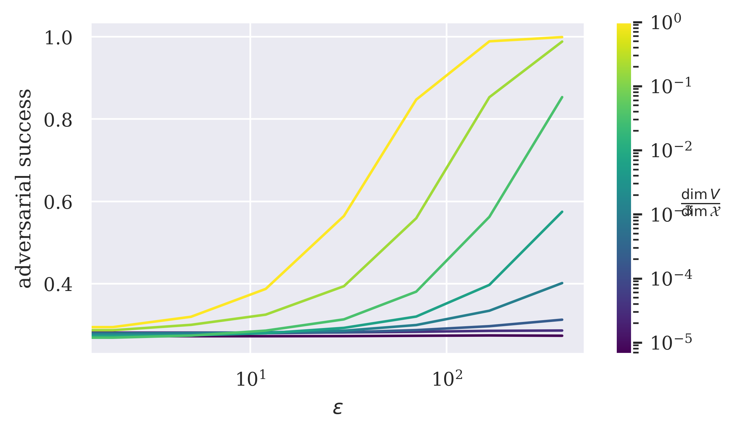
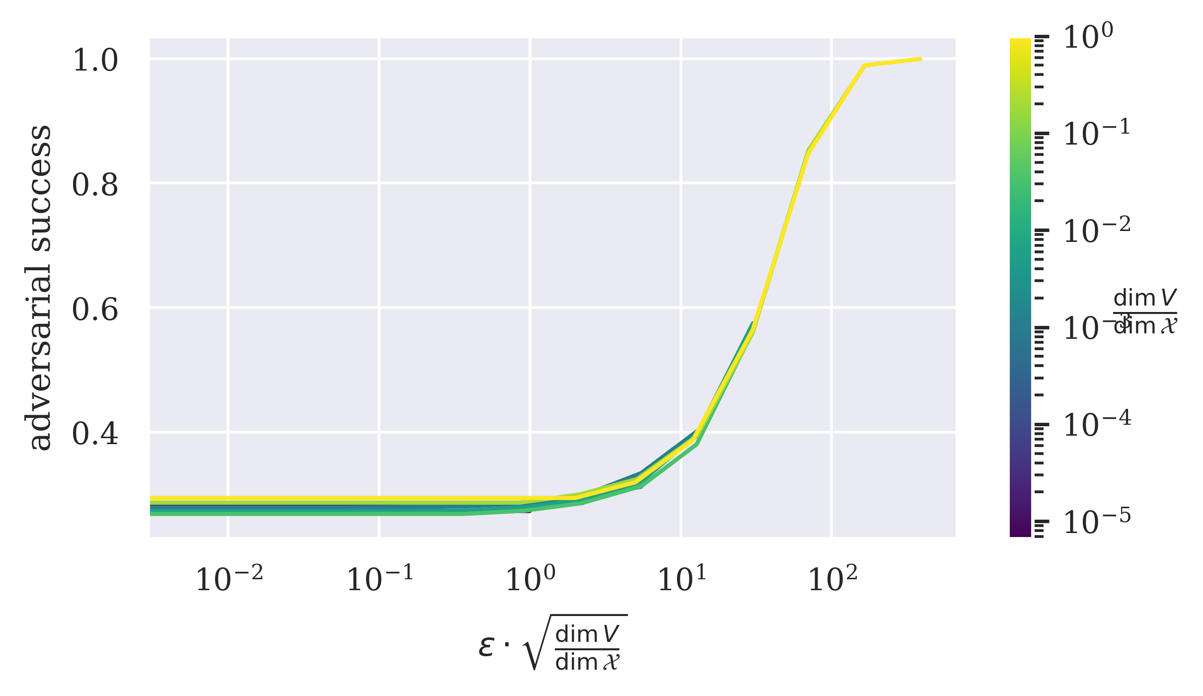
Figure 2: Top: success of PGD adversarial attacks on an ImageNet trained ResNet50, with $\ell^{2}$-norm constraints on perturbation budget (all other experimental details are as in Fig. 1, which displays analogous results for $\ell^{\infty}$-norm constraints). Left: these curves become aligned when we reparameterize the $x$-axis by scaling by $\sqrt{\frac{\dim V}{\dim\mathcal{X}}}$.

5.1 Datasets and models

We experiment with several image classification data sets and model architectures, of increasing image resolution and network capacity:

• The small convolutional network used in [23] trained on the MNIST dataset [22].

• A ResNet9 [16] trained on the CIFAR10 dataset [19].

• A ResNet50 [16] trained on the ImageNet dataset [7].

For further details on model architectures and training, we refer to Sec. B.1.

5.2 Functional form of adversarial success

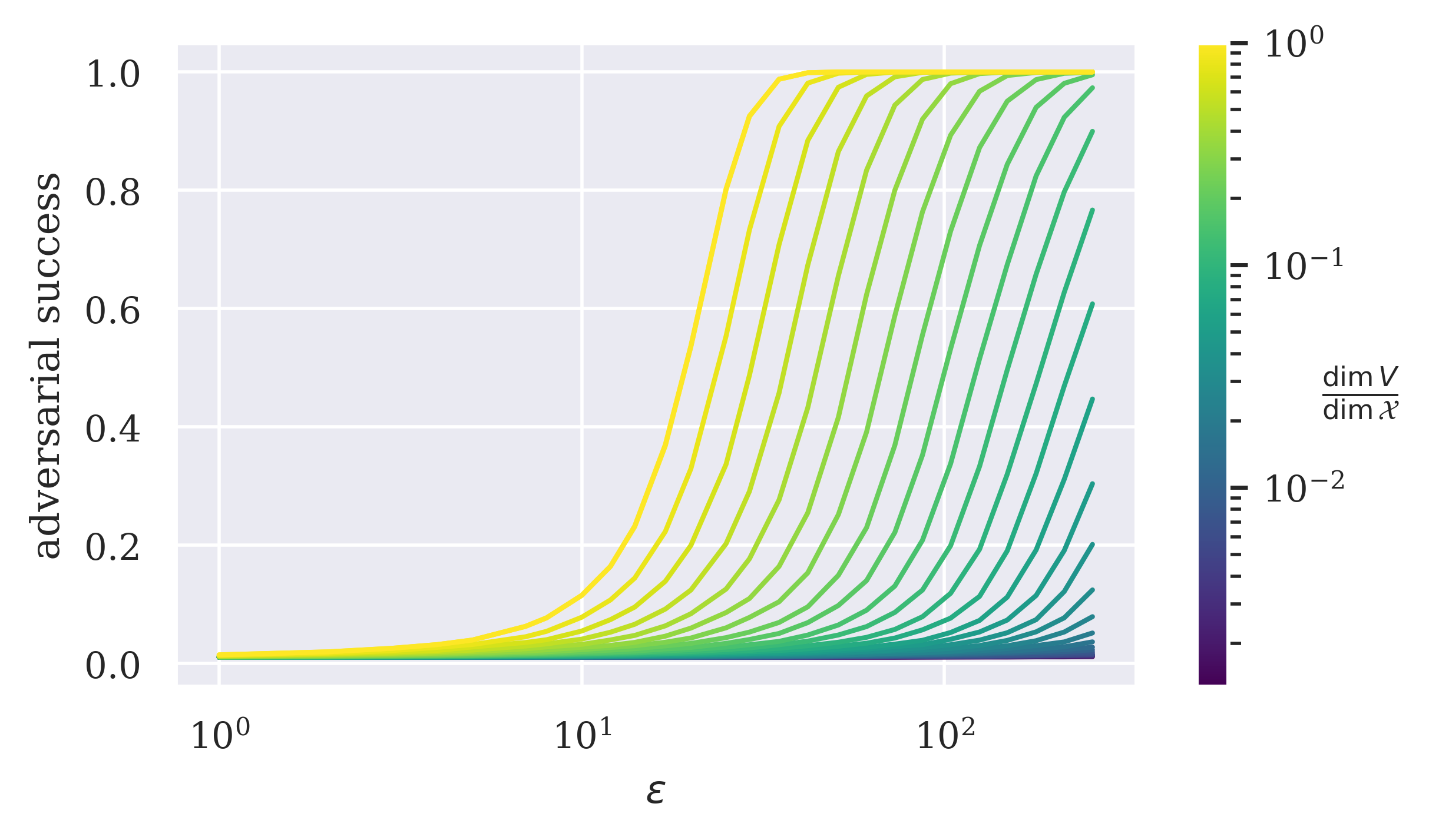
(a)

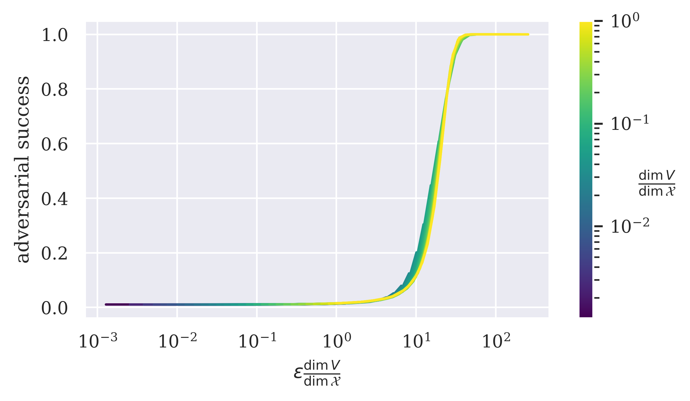
(b)

Figure 5: Plot for experiments analogous to those found in Figure 1 but run with a 2-layer CNN trained and evaluated on MNIST.

We may view the adversarial successes $\operatorname{success}(\dim V,\epsilon)$ as a sequence of functions of $\epsilon$, one for each $\dim V\in\{1,\dots,\dim\mathcal{X}\}$ as shown in the top plot of Fig. 1, which displays results of $\ell^{\infty}$ PGD adversarial attacks constrained to spans of subsets of standard basis vectors for a ResNet50 trained on ImageNet. It appears that for varying $\dim V$, the curves $\operatorname{success}(\dim V,\epsilon)$ differ by $x$-axis scalings, that is, transformations of the form $\operatorname{success}(\dim V,\epsilon)\leftarrow\operatorname{success}(\dim V,\lambda\epsilon)$ for some $\lambda>0$. This is indeed the case: the left plot in Fig. 1 shows that the curves $\operatorname{success}(\dim V,\epsilon\cdot\frac{\dim V}{\dim\mathcal{X}})$ are almost identical. Figures 5 and 6 show the same phenomena for a 2-layer CNN on MNIST and a ResNet9 on CIFAR10.

We can think of this analysis as expressing a decomposition $\operatorname{success}(\dim V,\epsilon)=g(\epsilon\cdot\frac{\dim V}{\dim\mathcal{X}})$ into a composition of two functions, the first being the map $(\dim V,\epsilon)\mapsto\epsilon\cdot\frac{\dim V}{\dim\mathcal{X}}$, the second map $g$ being some single-variable function applied to $\epsilon\cdot\frac{\dim V}{\dim\mathcal{X}}$. We do not attempt to identify this $g$.

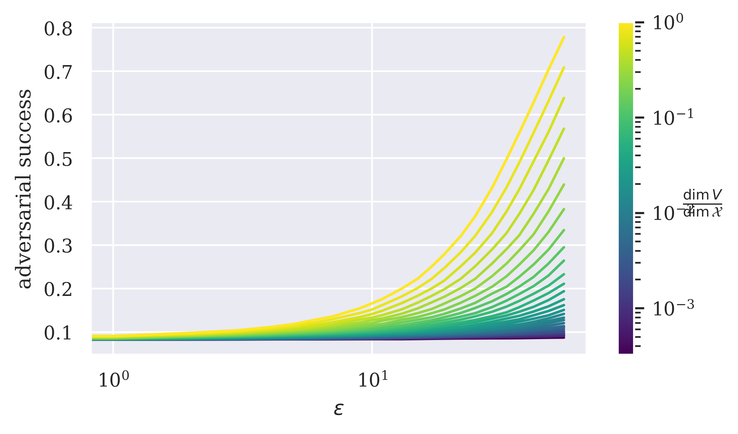
(a)

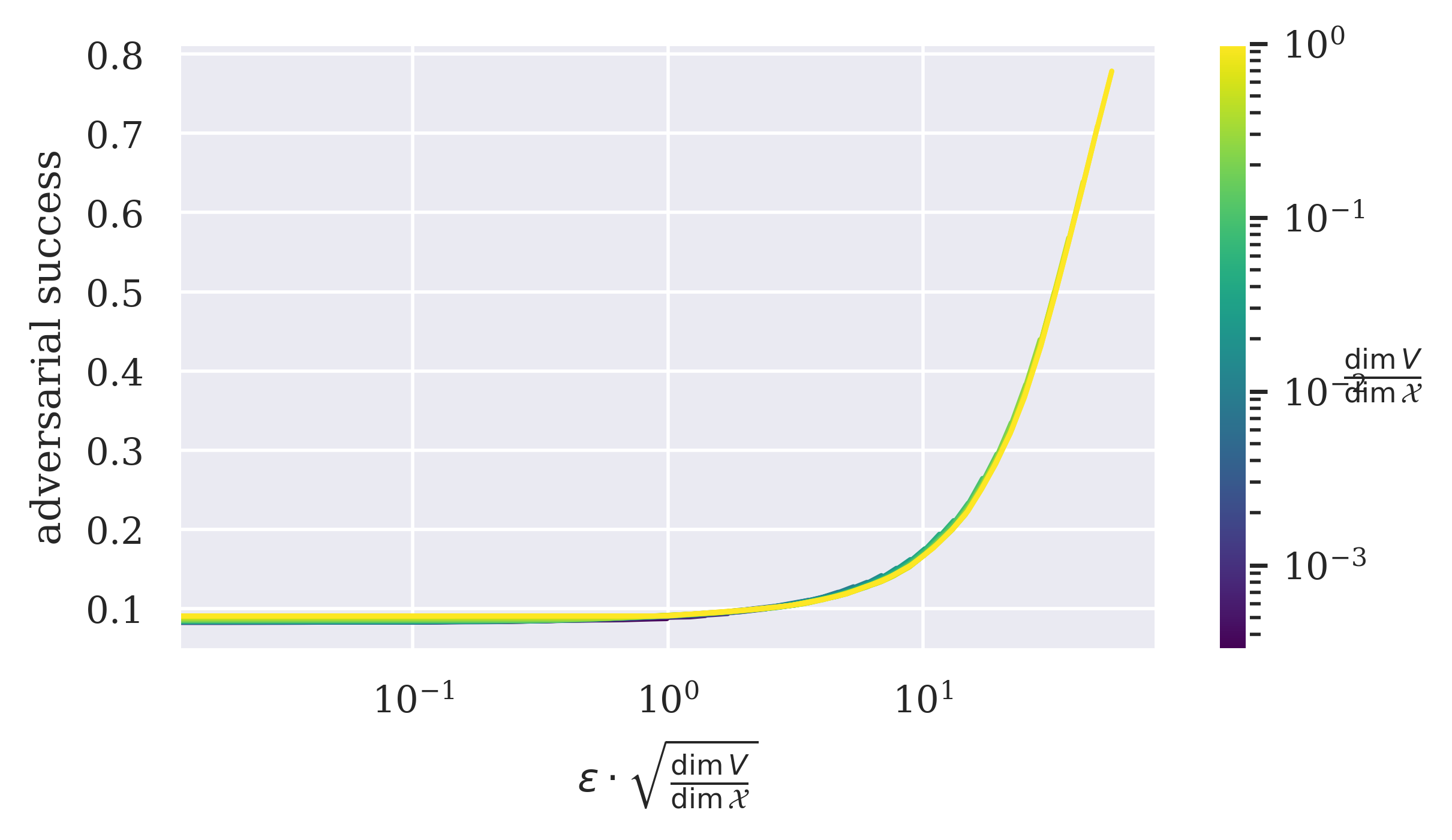
(b)

Figure 8: Plot for experiments analogous to those found in Figure 2 but run with a ResNet9 trained and evaluated on CIFAR10.

Figure 2 shows results analogous to those of Fig. 1 for PGD adversarial examples constrained in the $\ell^{2}$-norm (with plots for other architecture types and models in Figure 7 and Figure 8). In this case, the reparametrization of the $x$-axis that results in almost identical curves is obtained by replacing $\operatorname{success}(\dim V,\epsilon)$ with $\operatorname{success}(\dim V,\epsilon\cdot\sqrt{\frac{\dim V}{\dim\mathcal{X}}})$. This shows that the functional form of adversarial success in terms of $\epsilon$ and $\dim V$ depends on the norm constraining adversarial perturbations. In the following section, we argue that as long as $p>1$ adversarial success with $\ell^{p}$-constraints depends on $\epsilon d^{\frac{1}{q}}$ where $\frac{1}{p}+\frac{1}{q}=1$, a hypothesis consistent with experimental results in Fig. 2 and Fig. 1.

The case $p=1$ is more complicated, and we defer its analysis to Sec. B.5.

6 Comparison with existing theoretical predictions

There are many existing works investigating the mathematical source of adversarial examples for deep learning models. Several of these include (either as a main result or a byproduct of calculations) predictions for the functional form of adversarial success in terms of perturbation budget $\epsilon$ and the dimension $\dim V$ to which perturbations are constrained. We reviewed a subsample of such papers. Note that most of these papers (the exceptions being [10, 8]) focus on the dimension of the input space of a model alone and do not consider the additional constraint that adversarial examples are confined to a subspace.

1. From the analysis in [14] one can predict that adversarial success is a function of $\epsilon\frac{\dim V}{\dim X}$ (for $p=\infty$).

2. [10, 6, 8] predict that adversarial success is a function of $\epsilon(\frac{\dim V}{\dim\mathcal{X}})^{\frac{1}{2}}$ (for $p=2$).

3. From the analysis in [26, 31] one can predict that adversarial success is a function of $\epsilon(\frac{\dim V}{\dim\mathcal{X}})^{\frac{1}{q}}$ (for $\frac{1}{p}+\frac{1}{q}=1$). However, arriving at such a functional form from the derivations in [26, 31] requires multiple non-trivial steps not carried out in those works.

4. [29] predicts that adversarial success is a function of $\epsilon\dim V^{\frac{1}{2}-\frac{1}{\min(2,p)}}$.

The predictions of Items i, ii and iii are all consistent with our experimental results, suggesting that the situation where adversarial examples are constrained to a subspace of dimension $d$ is effectively equivalent to the unconstrained situation where data is found in an ambient space of dimension $d$. Those of Item iv are not obviously consistent with our experimental data, although we refrain from saying that they are inconsistent since the analysis of [29] involves a series of inequalities, and it is unclear how the predictions would change if one used slightly different approximations.

The dependence of adversarial success on $\epsilon(\frac{\dim V}{\dim\mathcal{X}})^{\frac{1}{q}}$ can be derived from the simplest possible toy model, namely binary linear classification. Let $\mathcal{X}=\mathbb{R}^{n}$ and suppose

$$f(x)=w^{T}x+b,\text{ for some }w\in\mathbb{R}^{n},b\in\mathbb{R}.$$ (6.1)

Let $V\subseteq\mathbb{R}^{n}$ be a subspace with $\dim V=d$. We will assume there exists an isometry $U:\mathbb{R}^{d}\xrightarrow{\simeq}V$ with respect to the $\ell^{p}$ metric. The point $x$ admits an $\ell^{p}$ adversarial example in the subspace $V$ with budget $\epsilon$, i.e. there is a $\delta\in V$ such that $\operatorname{sign}f(x+\delta)\neq\operatorname{sign}f(x)$ and $\lvert\delta\rvert_{p}\leq\epsilon$, if and only if the $\ell^{p}$ margin of $x$

$$\min_{\delta\in V}\big{\{}\lvert\delta\rvert_{p}\;\big{|}\;f(x+\delta)=0\big{\}}$$ (6.2)

is at most $\epsilon$.

Lemma 6.3.

With the above definitions and notation and with $\frac{1}{p}+\frac{1}{q}=1$,

$$\min_{\delta\in V}\big{\{}\lvert\delta\rvert_{p}\;\big{|}\;f(x+\delta)=0\big{\}}=\frac{\lvert w^{T}x+b\rvert}{\lvert w^{T}U\rvert_{q}}.$$ (6.4)

Appendix A contains a proof. Our experimental results only measure the probability that $x$ admits an $\ell^{p}$-adversarial example in the subspace $V$ with budget $\epsilon$. By the above lemma, this probability is $P(\frac{\lvert w^{T}x+b\rvert}{\lvert w^{T}U\rvert_{q}}\leq\epsilon)$, which can be rewritten as $P(\lvert w^{T}x+b\rvert\leq\epsilon\lvert w^{T}U\rvert_{q})$. We claim that when $p>1$ and $V$ (equivalently $U$) is sampled with sufficient randomness

$$\mathbb{E}\big{[}\lvert w^{T}U\rvert_{q}\big{]}=\Big{(}\frac{d}{n}\Big{)}^{\frac{1}{q}}\lvert w\rvert_{q}.$$ (6.5)

In the case where $V$ is generated by a subset, say $\{e_{i_{1}},\dots,e_{i_{d}}\}$ of basis vectors, this can be argued as follows:

$$\begin{split}\frac{\lvert w^{T}U\rvert_{q}^{q}}{\lvert w\rvert_{q}^{q}}&=\frac{\sum_{j=1}^{d}\lvert w_{i_{j}}\rvert^{q}}{\sum_{i=1}^{n}\lvert w_{i}\rvert^{q}}\\ &=\frac{d}{n}\frac{\frac{1}{d}\sum_{j=1}^{d}\lvert w_{i_{j}}\rvert^{q}}{\frac{1}{n}\sum_{i=1}^{n}\lvert w_{i}\rvert^{q}}\\ \end{split}$$ (6.6)

When the basis subset $\{e_{i_{1}},\dots,e_{i_{d}}\}$ is sampled uniformly we claim that that the expectation of the term $\frac{1}{d}\sum_{j=1}^{d}\lvert w_{i_{j}}\rvert^{q}$ is exactly $\frac{1}{n}\sum_{i=1}^{n}\lvert w_{i}\rvert^{q}$ (at least when $d=1$ this is immediate). Thus after averaging over many random subspaces $V$,

$$\mathbb{E}\Big{[}\frac{\frac{1}{d}\sum_{j=1}^{d}\lvert w_{i_{j}}\rvert^{q}}{\frac{1}{n}\sum_{i=1}^{n}\lvert w_{i}\rvert^{q}}\Big{]}=1,\text{ hence }\mathbb{E}\Big{[}\frac{\lvert w^{T}U\rvert_{q}^{q}}{\lvert w\rvert_{q}^{q}}\Big{]}=\frac{d}{n}.$$ (6.7)

Taking $q$-th roots and rearranging gives Eq. 6.5.

Note that in our experiments we compute something analogous to $P(\lvert w^{T}x+b\rvert\leq\epsilon\lvert w^{T}U\rvert_{q})$ where probability is with respect to the underlying distribution of $x$ and choice of $U$. Using a “point estimate” and replacing $\lvert w^{T}U\rvert_{q}$ with its mean $(\frac{d}{n})^{\frac{1}{q}}\lvert w\rvert_{q}$, one would simplify to $P(\lvert w^{T}x+b\rvert\leq\epsilon(\frac{d}{n})^{\frac{1}{q}}\lvert w\rvert_{q})$, which since we treat $w,b$ and the distribution of $x$ as given is a function of $\epsilon(\frac{d}{n})^{\frac{1}{q}}$.

When $p=1$, so $q=\infty$, Lemma 6.3 remains valid but the tricks applied in Eqs. 6.6 and 6.7 do not make sense, and indeed our experimental results in Sec. B.5 suggest dependence of adversarial success on $\epsilon(\frac{\dim V}{\dim\mathcal{X}})^{\frac{1}{q}}$ alone breaks down somewhat in this case. For further analysis of this case, we refer to Sec. B.5.

7 Limitations

Adversarial examples given by gradient-based perturbations with $\ell^{p}$ constraints make up only one (and arguably, a narrow) type of distribution-shifted test data causing machine learning model failure. For further discussion of this point see [12, 13]. While we take inspiration from adversarial example generators constraining perturbations to subspaces (surveyed in Sec. 2), our experiments are limited to the baseline of random subspace selection (whereas most subspace-constrained adversarial example generators choose their subspace more carefully). We also only experiment with image classifiers, though adversarial examples have been found to exist for essentially all deep learning systems [25, 20, 37].

8 Conclusion and open questions

We demonstrate that the adversarial success $\operatorname{success}(\dim V,\epsilon)$ of PGD attacks constrained to a (random) $\dim V$-dimensional subspace $V$ of the model input space $\mathcal{X}$ with $\ell^{p}$ budget $\epsilon$ (and $p>1$) is essentially a function of the single variable $\epsilon(\frac{\dim V}{\dim\mathcal{X}})^{\frac{1}{q}}$ where $\frac{1}{p}+\frac{1}{q}=1$ (rather than a function of two variables as considered in prior work). The fact that this relationship can be derived in the toy example of a linear binary classifier, and holds quite sharply in all our experiments, seems to lend further credence to the theory that adversarial examples are a byproduct of the locally linear behavior of neural networks with high dimensional input spaces.

Acknowledgments

The research described in this paper was conducted under the Laboratory Directed Research and Development Program at Pacific Northwest National Laboratory, a multiprogram national laboratory operated by Battelle for the U.S. Department of Energy.

Appendix A Derivations

Proof of Lemma 6.3.

Recall that our goal is to solve the constrained optimization problem

$$\min\{\lvert\delta\rvert_{p}\,|\,\delta\in\mathbb{R}^{d},w^{T}(x+U\delta)+b=0\}$$ (A.1)

Using the method of Lagrange multipliers, we know that a minimizer $\delta\in\mathbb{R}^{d}$ must satisfy the critical point condition

$$\lambda U^{T}w\in\partial\lvert\delta\rvert_{p}$$ (A.2)

where $\partial\lvert\delta\rvert_{p}$ is the subdifferential of the $\ell^{p}$-norm at $\delta\in\mathbb{R}^{d}$. It is a classical fact (see e.g. [1, Prop. 1.2]) that

$$\partial\lvert\delta\rvert_{p}=\begin{cases}\{v\in\mathbb{R}^{d}\,|\,\lvert v\rvert_{q}\leq 1\}&\text{if }\delta=0\\ \{v\in\mathbb{R}^{d}\,|\,\lvert v\rvert_{q}=1\text{ and }v^{T}\delta=\lvert\delta\rvert_{p}\}&\text{otherwise.}\end{cases}$$ (A.3)

If the first case occurs, clearly the minimum of Eq. A.1 is $0$, and since $\delta=0$ we obtain

$$0=w^{T}(x+U\delta)+b=w^{T}x+b,$$ (A.4)

hence in this case $\frac{\lvert w^{T}x+b\rvert}{\lvert w^{T}U\rvert_{q}}=0$ as well and the lemma holds.

In the case where $\delta\neq 0$, combining Eqs. A.2 and A.3 we see that for some $\lambda$

$$\lvert\lambda U^{T}w\rvert_{q}=1\text{ and }\lambda w^{T}U\delta=\lvert\delta\rvert_{p};$$ (A.5)

from the first equation we immediately identify $\lvert\lambda\rvert=\lvert U^{T}w\rvert_{q}^{-1}$, and taking absolute values on both sides of the second then gives

$$\begin{split}\lvert\delta\rvert_{p}&=\lvert\lambda\rvert\lvert w^{T}U\delta\rvert\\ &=\frac{\lvert w^{T}U\delta\rvert}{\lvert U^{T}w\rvert_{q}}.\end{split}$$ (A.6)

Finally, recalling $w^{T}(x+U\delta)+b=0$ gives $\lvert w^{T}U\delta\rvert=\lvert w^{T}x+b\rvert$, completing the proof. ∎

Appendix B Experimental details

B.1 Model architectures and training details

For our MNIST experiments we use the simple 2 layer convolutional network of [23] — we ported the TensorFlow code available at https://github.com/MadryLab/mnist_challenge to PyTorch [27]. We train it using SGD with momentum 0.9, batch size $1024$ and weight decay $10^{-4}$ for 100 epochs, with initial learning rate $10^{-3}$ and learning rate drops by a factor of $0.1$ whenever validation accuracy doesn’t improve by $1\%$ for 10 epochs. We save the weights with the best validation accuracy ($\approx 98.95\%$).

For our CIFAR10 experiments we use the ResNet9 from MosaicML’s Composer library [34]. We train it with SGD with momentum 0.9, batch size $512$ and weight decay $10^{-4}$ for 160 epochs, with initial learning rate $10^{-1}$ and learning rate drops by a factor of $0.1$ whenever validation accuracy doesn’t improve by $1\%$ for 10 epochs. We save the weights with the best validation accuracy ($\approx 91.72\%$).

For our ImageNet experiments we use the ResNet50 from TorchVision [24]. We train it with SGD with momentum 0.9 and weight decay $10^{-4}$ for 100 epochs, with initial learning rate $1.0$ and learning rate drops by a factor of $0.1$ whenever validation accuracy doesn’t improve by $1\%$ for 10 epochs. Due to distributed data parallel training with batches of size 512 on each of 8 GPUs, our effective batch size is $8\cdot 512=4096$. We save the weights with the best validation accuracy ($\approx 72.84\%$).

B.2 Tuning PGD step sizes

In our experiments we generate a large number of PGD adversarial examples for a wide range of perturbation constraints $\epsilon$ and in subspaces of varying dimension. In order for our numerical experiments to address our questions about the behavior of $\operatorname{success}(d,\epsilon)$, it is crucial that our PGD algorithm for optimizing $\delta$ has the capacity to achieve the boundary case $\lvert\delta\rvert_{p}=\epsilon$. We found that with some standard choices of step size, this did not occur, resulting in an unpleasant situation where the effective budget was significantly lower than $\epsilon$ simply due to a too-small PGD step size. Here we briefly discuss a principled choice of PGD step size that accounts for the dimension $d$ of the subspace to which $\delta$ is constrained. First we must specify the PGD algorithm being used.

Our basic PGD implementation (adapted from [23]) iterates the following: we constrain $\delta$ to a $d$-dimensional subspace $V\subseteq\mathcal{X}$ using an isometry $U:\mathbb{R}^{d}\to V$ as in Sec. 6, and initialize $\delta_{0}=0$ . Then, for $t=1,\dots,T$ where $T$ is the maximum number of steps, we let $g_{t}=\nabla_{\delta}\ell(f(x+U\delta),y)$ where $\ell$ is cross entropy, and replace it with the “normalized” gradient

$$\tilde{g}_{t}:=\begin{cases}\frac{g_{t}}{\lvert g_{t}\rvert_{p}},&p\in\{1,2\}\\ \operatorname{sign}{g_{t}},&p=\infty.\end{cases}$$ (B.1)

We then project $\delta_{t-1}+\eta\tilde{g}_{t}$, where $\eta$ is a learning rate, onto the $\ell^{p}$ $\epsilon$-ball centered at $0$ to obtain in the case $p\in\{1,2\}$

$$\delta_{t}=\begin{cases}\epsilon\frac{\delta_{t-1}+\eta\tilde{g}_{t}}{\lvert\delta_{t-1}+\eta\tilde{g}_{t}\rvert_{p}},&\lvert\delta_{t-1}+\eta\tilde{g}_{t}\rvert_{p}>\epsilon\\ \delta_{t-1}+\eta\tilde{g}_{t},&\text{otherwise}\end{cases}$$ (B.2)

and in the case $p=\infty$

$$\delta_{t}=\begin{cases}\epsilon\frac{\delta_{t-1}+\eta\tilde{g}_{t}}{\max\{\delta_{t-1}+\eta\tilde{g}_{t}\}},&\max\{\delta_{t-1}+\eta\tilde{g}_{t}\}>\epsilon\\ \delta_{t-1}+\eta\tilde{g}_{t},&\text{otherwise}.\end{cases}$$ (B.3)

Finally, we must ensure that $x+U\delta$ lies in the image hypercube $[0,1]^{C\times H\times W}$ (in our implementation pixel values lie in $[0,1]$). To do this, we let $\operatorname{clip}:\mathbb{R}\to[0,1]$ be the clipping function, i.e. $\operatorname{clip}(x)=\max\{0,\min\{x,1\}\}$, and replace $\delta$ with

$$U^{T}(\operatorname{clip}(x+U\delta)-x)$$ (B.4)

(here we use the fact that $U$ is orthogonal and so $U^{T}$ is a left inverse for $U$).

To set the step size $\eta$, we can adopt the heuristic that the $\delta_{t}$ behave like a random walk, i.e. that the normalized gradients $\tilde{g}_{t}$ are sampled IID from some distribution (this almost certainly quite false, but we found it to be useful in a back-of-the-envelope sort of way). We will even further assume that for each $t$ the coordinates of $\tilde{g}_{t}$ are IID. Ignoring projection and clipping, we have $\delta_{T}=\eta\sum_{t=1}^{T}\tilde{g}_{t}$. In the case $p=2$, using the supposed IID-ness we see that

$$E[\lvert\delta\rvert_{2}^{2}]=\eta^{2}\sum_{t=1}^{T}\lvert\tilde{g}_{t}\rvert_{2}^{2}=\eta^{2}T.$$ (B.5)

Since we want to ensure the left hand side is at least $\epsilon$, we obtain the step size

$$\eta=\frac{\epsilon}{\sqrt{T}}.$$ (B.6)

In practice we multiply the above by 2 for good measure. In the case $p=\infty$, by our IID-ness assumptions and the fact that by definition $\tilde{g}_{t}=\operatorname{sign}{g_{t}}$, the individual coordinates $\tilde{g}_{t,j}$ for $j=1,\dots,d$ are IID samples from $\{\pm 1\}$ and so

$$\lvert\delta_{T}\rvert_{\infty}=\eta\sqrt{T}\max_{j=1,\dots,d}\{\lvert\frac{1}{\sqrt{T}}\sum_{t=1}^{T}\tilde{g}_{t,j}\rvert\}$$ (B.7)

The distribution of each term $\frac{1}{\sqrt{T}}\sum_{t=1}^{T}\tilde{g}_{t,j}$ tends towards a Gaussian distribution with mean 0 and variance $1$ as $T\to\infty$ by the central limit theorem. Letting $\Phi(x)$ be the standard normal CDF, the CDF of each $\lvert\frac{1}{\sqrt{T}}\sum_{t=1}^{T}\tilde{g}_{t,j}\rvert$ is approximated by

$$F(x):=\Phi(x)-\Phi(-x).$$ (B.8)

By [2], the distribution of the max occuring in Eq. B.7 is concentrated around the $\frac{d-1}{d}$-th quantile of the CDF Eq. B.8, i.e. $F^{-1}(1-\frac{1}{d})$. Assuming $d$ is relatively large, so that $1-\frac{1}{d}$ is near $1$, we ignore the $\Phi(-x)$ term in Eq. B.8 for the purposes of inversion and get

$$F^{-1}(1-\frac{1}{d})\approx\Phi^{-1}(1-\frac{1}{d})$$ (B.9)

Recall that our objective is to ensure that $\lvert\delta_{T}\rvert_{\infty}\geq\epsilon$. By the above arguments, this translates to

$$\begin{split}\epsilon&\leq\eta\sqrt{T}\Phi^{-1}(1-\frac{1}{d}),\text{ i.e. }\\ \eta&\approx\frac{\epsilon}{\sqrt{T}\Phi^{-1}(1-\frac{1}{d})}.\end{split}$$ (B.10)

Again, in practice we multiply by 2 for good measure. Observe that while our $\ell^{2}$ step size is independent of $d$, Eq. B.10 does depend on $d$. In fact, as $d\to\infty$ the step size goes to $0$, but very slowly (for $d=3\cdot 224^{2}$, the dimension of ImageNet images, $\Phi^{-1}(1-\frac{1}{d})\approx 4.36$).

For the $p=1$ case, we use a heuristic similar to that of $p=2$ above; explicitly, we set

$$\eta=\sqrt{2\pi}\frac{\epsilon}{\sqrt{T}}$$

B.3 Adversarial example generation

For each dataset and model, we select a range of perturbation budgets $\epsilon$ and subspace dimensions $d$, in both cases logarithmically spaced between minimum and maximal values of $\epsilon$ and $d$, with as many grid points as we can afford (for MNIST and CIFAR, 32 different values of each, for ImageNet only 8 of each).

For each pair $(\epsilon,d)$ we loop over the entire validation set of the relevant dataset, with the exception of ImageNet where we randomly sample 10,000 of the 50,000 images. We randomly sample a distinct subspace $V_{i}\subset\mathcal{X}$ for each validation datapoint $(x_{i},y_{i})$ (as above, by randomly generating a matrix $U$ whose columns span $V$). We then loop through validation datapoints $(x_{i},y_{i})$ and corresponding matrices $U_{i}$ and compute PGD adversarial examples as described above, with $T=16$ steps. We compute the error over the validation set (subsampled in the case of ImageNet), i.e.

$$1-\frac{1}{N}\sum_{i=1}^{N}\mathbf{1}(f(x_{i}+U\delta_{i})=y_{i}).$$

B.4 Subspaces sampled uniformly from the Grassmannian

In the case of MNIST and for $p=2$, we can also sample subspaces uniformly from the Grassmannian $\operatorname{Gr}(d,\dim\mathcal{X})$ by sampling matrices $U$ of shape $n\times d$ with orthonormal columns using the QR decomposition as in used in the method scipy.stats.ortho_group of [36]. The results, shown in Fig. 3, are similar to those in Figs. 5(a) and 5(b).

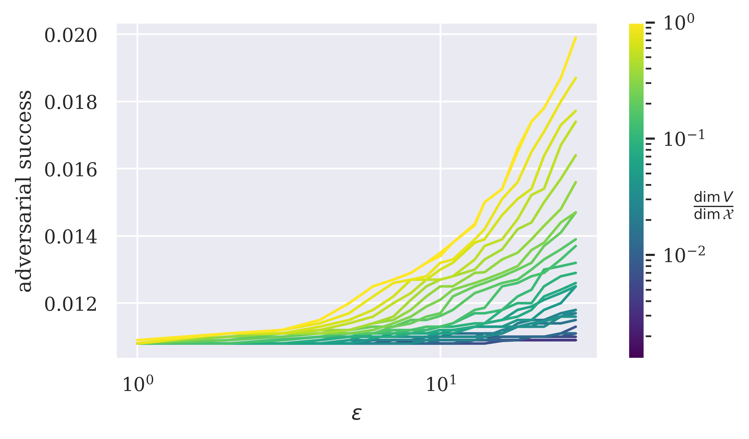
(a)

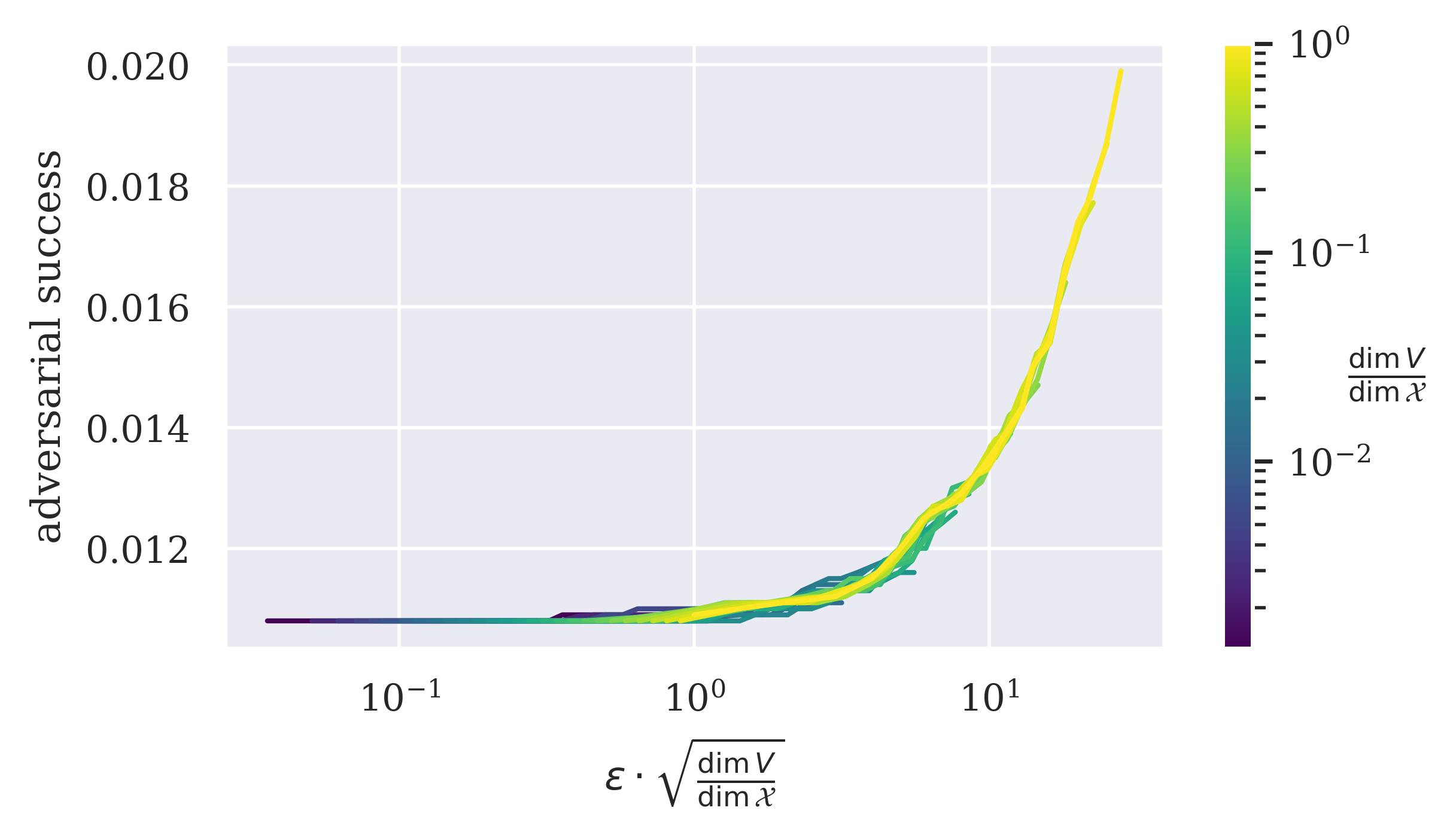
(b)

Figure 3: (a) Projected gradient descent (PGD) adversarial examples for the 2-layer convolutional neural network of [23] on the MNIST validation set. In these experiments we generated the subspaces $V$ by sampling uniformly from the Grassmannian, and constrain perturbations using the $\ell^{2}$ norm. (b) The same data, reparametrized by plotting $\epsilon\cdot\sqrt{\frac{\dim V}{\dim\mathcal{X}}}$ along the $x$-axis. Note: $x$-axes are log-scale.

B.5 Analysis of the 1-norm case

When $p=1$, $q=\infty$ and so the arguments used in Eqs. 6.6 and 6.7 do not make sense as written; moreover, while we have not explicitly verified this, it seems that attempting to take a limit of those equations as $q\to\infty$ one will encounter an “$\infty/\infty$” case, and it’s not clear that e.g. L’Hospital’s rule helps at all.

Instead, we propose a different estimate of the quotient

$$\frac{\lvert w^{T}U\rvert_{\infty}}{\lvert w\rvert_{\infty}},$$ (B.11)

proceeding as follows. We will again assume, as is the case in our experiments, that $U$ is obtained by subsampling basis vectors, say $\{e_{i_{1}},\dots,e_{i_{d}}\}$. Then

$$\frac{\lvert w^{T}U\rvert_{\infty}}{\lvert w\rvert_{\infty}}=\frac{\max_{j}\{\lvert w_{i_{j}}\rvert\}}{\max_{i}\{\lvert w_{i}\rvert\}}$$ (B.12)

The question, then, is how much smaller the $\max$ over a random $\dim V$-element subset of the absolute values $\lvert w_{i}\rvert$ is than the $\max$ over all $\dim\mathcal{X}$ of them. The need to make some assumption on the distribution the $\lvert w_{i}\rvert$ are drawn from seems unavoidable at this point: we suppose the coefficients $w_{i}$ come from a standard normal distribution, so that their absolute values come from a “half-normal” (equivalently $\chi_{1}$) distribution: if $\Phi$ is the standard normal cumulative distribution function, with this assumption the cumulative distribution function of the $\lvert w_{i}\rvert$ is

$$F(x):=\Phi(x)-\Phi(-x).$$ (B.13)

We make a further crude estimate that the numerator and denominator are $\max$s of independent samples of size $\dim V$ and $\dim\mathcal{X}$ respectively; then the theory of quantiles in large samples [2] suggests the estimates

$$\begin{split}\max_{j}\{\lvert w_{i_{j}}\rvert\}&\approx F^{-1}(1-\frac{1}{\dim V})\text{ and}\\ \max_{i}\{\lvert w_{i}\rvert\}&\approx F^{-1}(1-\frac{1}{\dim\mathcal{X}})\end{split}$$ (B.14)

leading to the overall estimate

$$\frac{\lvert w^{T}U\rvert_{\infty}}{\lvert w\rvert_{\infty}}\approx\frac{F^{-1}(1-\frac{1}{\dim V})}{F^{-1}(1-\frac{1}{\dim\mathcal{X}})}$$ (B.15)

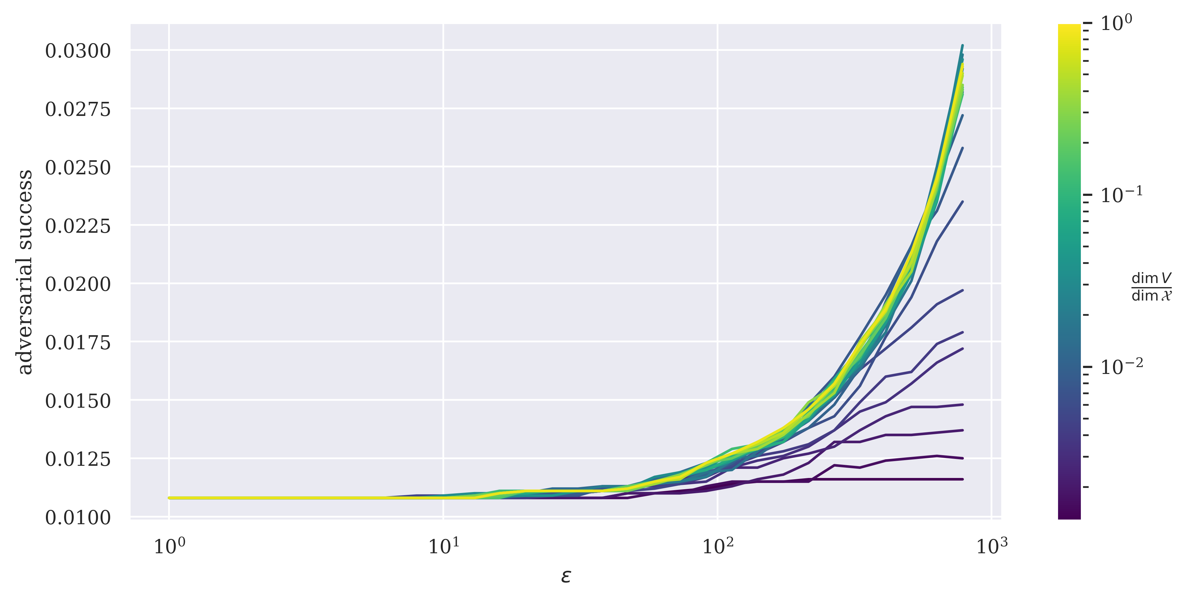
(a)

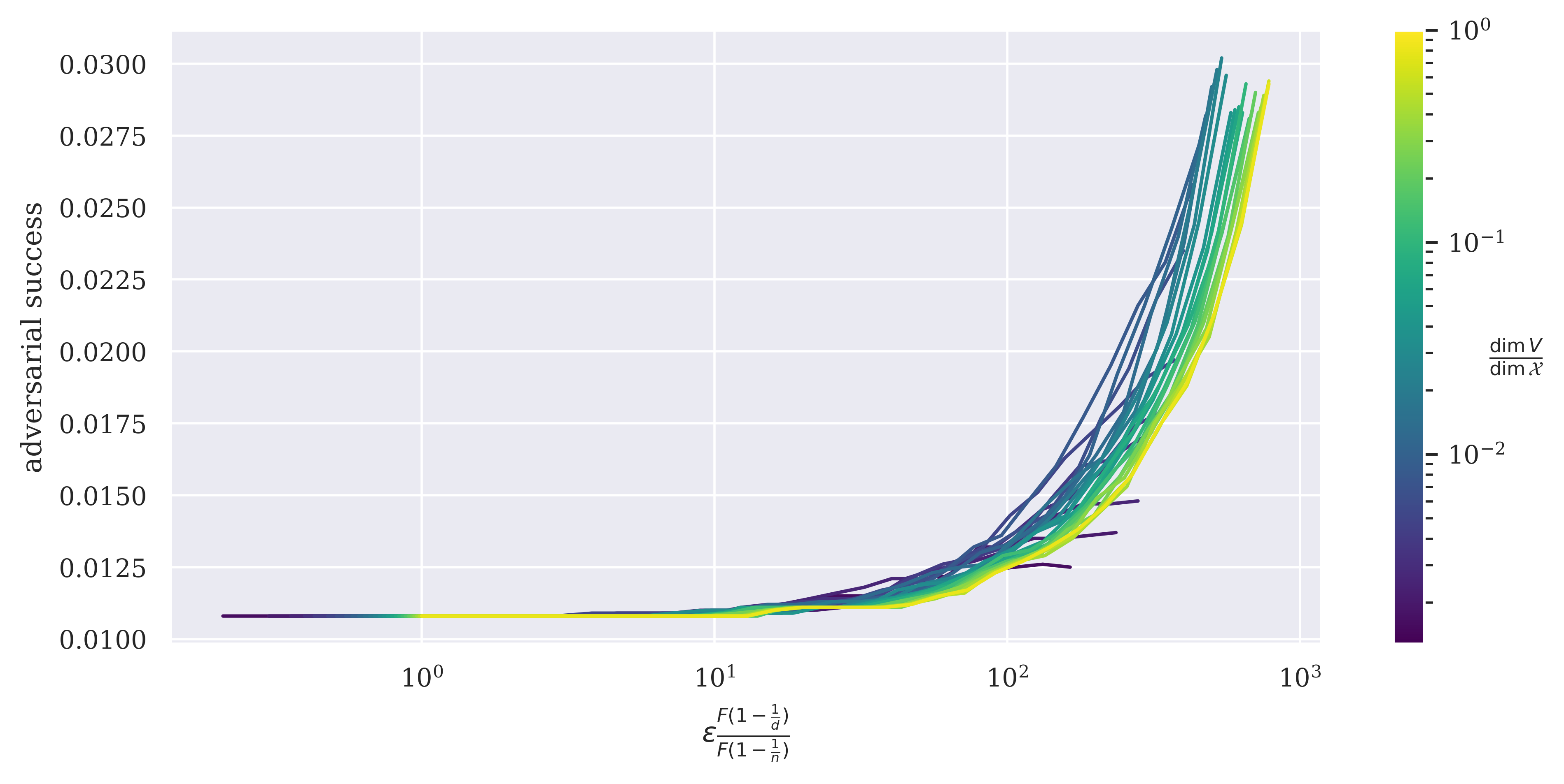
(b)

Figure 4: (a) Success of PGD adversarial attacks on an MNIST trained small convolutional network, with $\ell^{1}$-norm constraints on perturbation budget, constrained to subspaces $V\subseteq\mathcal{X}$ spanned by $\dim V$ randomly selected standard basis vectors. Adversarial examples are computed for all datapoints in the MNIST validation set. The $x$-axis is the $\epsilon$-bound used during example generation and the different colored curves indicate the dimension $\dim V$ of the subspace to which the examples were constrained to, relative to the dimension $\dim\mathcal{X}$ ($=28^{2}$) of the ambient space. (b) These curves become more aligned when we reparameterize the $x$-axis by scaling by $\frac{F(1-\frac{1}{\dim V})}{F(1-\frac{1}{\dim\mathcal{X}})}$, where $F$ is the cummulative distribution function of the absolute value of a standard normal random variable.

Figure 4 shows the result of using Eq. B.15 as a stand-in for $(\frac{\dim V}{\dim\mathcal{X}})^{\frac{1}{q}}$ in the case where $p=1$, on the MNIST dataset. One immediate observation is that at least for $\dim V$ a significant fraction of $\dim\mathcal{X}$ (e.g. $\frac{\dim V}{\dim\mathcal{X}}\geq 0.1$) it does appear that the curves $\operatorname{success}(\dim V,\epsilon)$ converge to a common limit, as one would expect from a naïve application of a factorization $\operatorname{success}(\dim V,\epsilon)=g(\epsilon(\frac{\dim V}{\dim\mathcal{X}})^{\frac{1}{\infty}})=g(\epsilon)$. The reparameterization of Eq. B.15 seems to do okay at accounting for behavior in the lowest dimensions, at the expense of over-compensating and pushing the curves corresponding to low-to-medium values of $\dim V$ to the left of the curve corresponding to $\dim V=\dim\mathcal{X}$. There are various potential causes of this undesirable effect (roughly one per crude oversimplification in the above analysis). Results for CIFAR10 and ImageNet can be found in Fig. 9 and Fig. 10 respectively. One concerning aspect of those two results is we see downturns in the curves $\operatorname{success}(\dim V,\epsilon)$ for the highest values of $\epsilon$, suggesting there may have been issues with our PGD optimizer in the $p=1$ case.

One question we had was whether these results were impacted by sub-optimal PGD optimization. A reason for asking this is that the $p=1$ case of Eq. B.1 is arguably incorrect: the “correct” way of deriving these generalized Fast Gradient Sign Method (FGSM) steps is through the analysis of Appendix A. Assuming $U=I$ for simplicity, one sees that $w^{T}\delta=\lvert w\rvert_{\infty}\lvert\delta\rvert_{1}$, and one can show this occurs if and only if:

• letting $A=\mathrm{arg}\max_{i}\{\lvert w_{i}\rvert\}\subseteq\{1,\dots,n\}$ (the argmax of $\lvert w_{i}\rvert$, which is a set in general although a single index with probability 1), $\delta_{i}=0$ if $i\notin A$.

• $\operatorname{sign}\delta_{i}=\operatorname{sign}w_{i}$ for all $i\in A$.

In the case where $A=\{a\}$ (i.e. $\lvert w_{i}\rvert$ has a unique maximum) we obtain the simplified solution $\delta=(c\operatorname{sign}w_{i})e_{a}$ (where $e_{a}$ is the $a$-th standard basis vector. Hence for $p=1$, one can argue that we should use

$$\tilde{g}_{t}:=e_{\mathrm{arg}\max_{i}\{\lvert w_{i}\rvert\}}$$ (B.16)

We found that while this method performed similarly to that of Eq. B.1 for small values of $\epsilon$, it struggled for large $\epsilon$ and failed at the scale of ImageNet input space (see). A reasonable suspicion is that the number of basis directions selected by Eq. B.16 is bounded by the number of PGD iterations, and that when this number of iterations is far is smaller than the input dimension Eq. B.16 underexplores. However we leave further analysis to future work.

Appendix C Additional experimental results

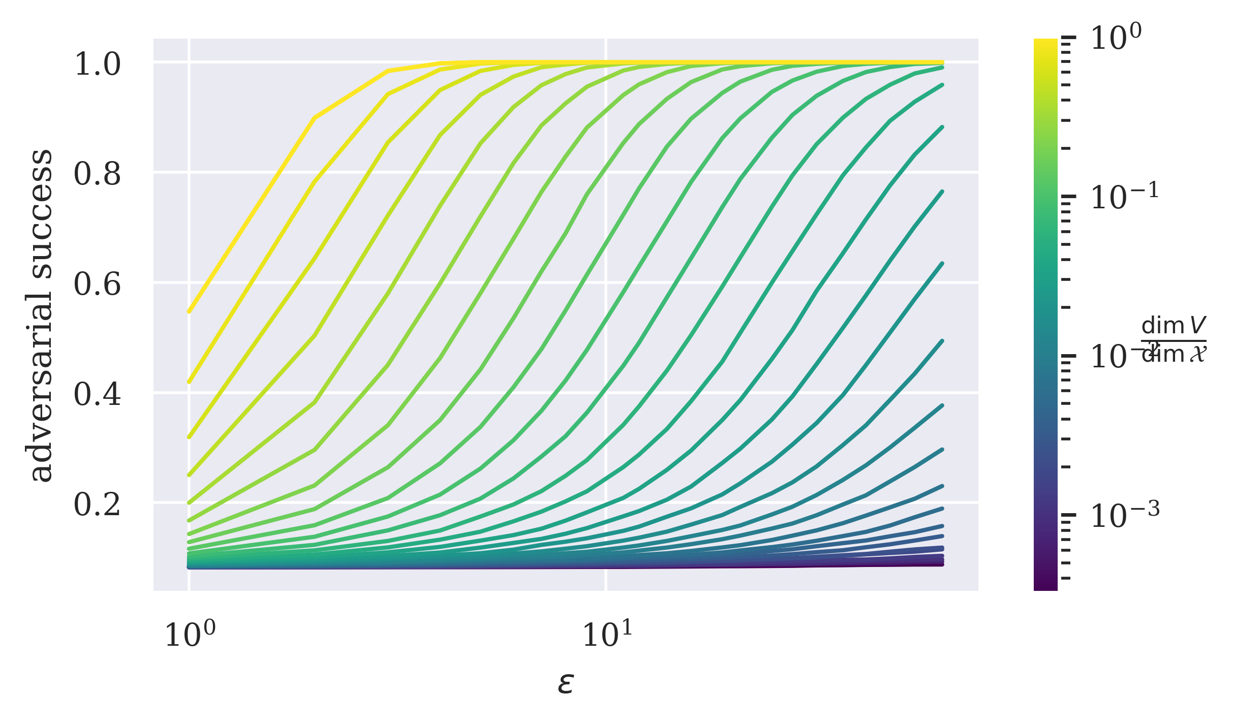
(a)

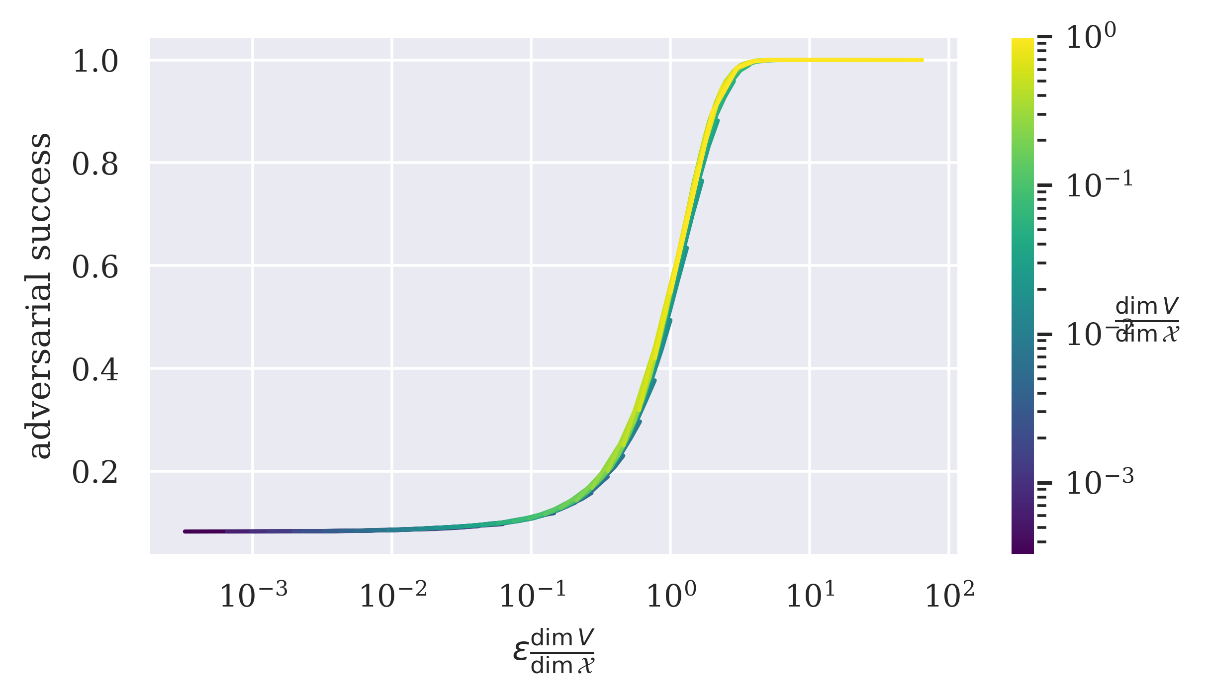
(b)

Figure 6: Plot for experiments analogous to those found in Figure 1 but run with a ResNet9 trained and evaluated on CIFAR10.

(a)

(b)

Figure 7: Plot for experiments analogous to those found in Figure 2 but run with a 2-layer CNN trained and evaluated on MNIST.

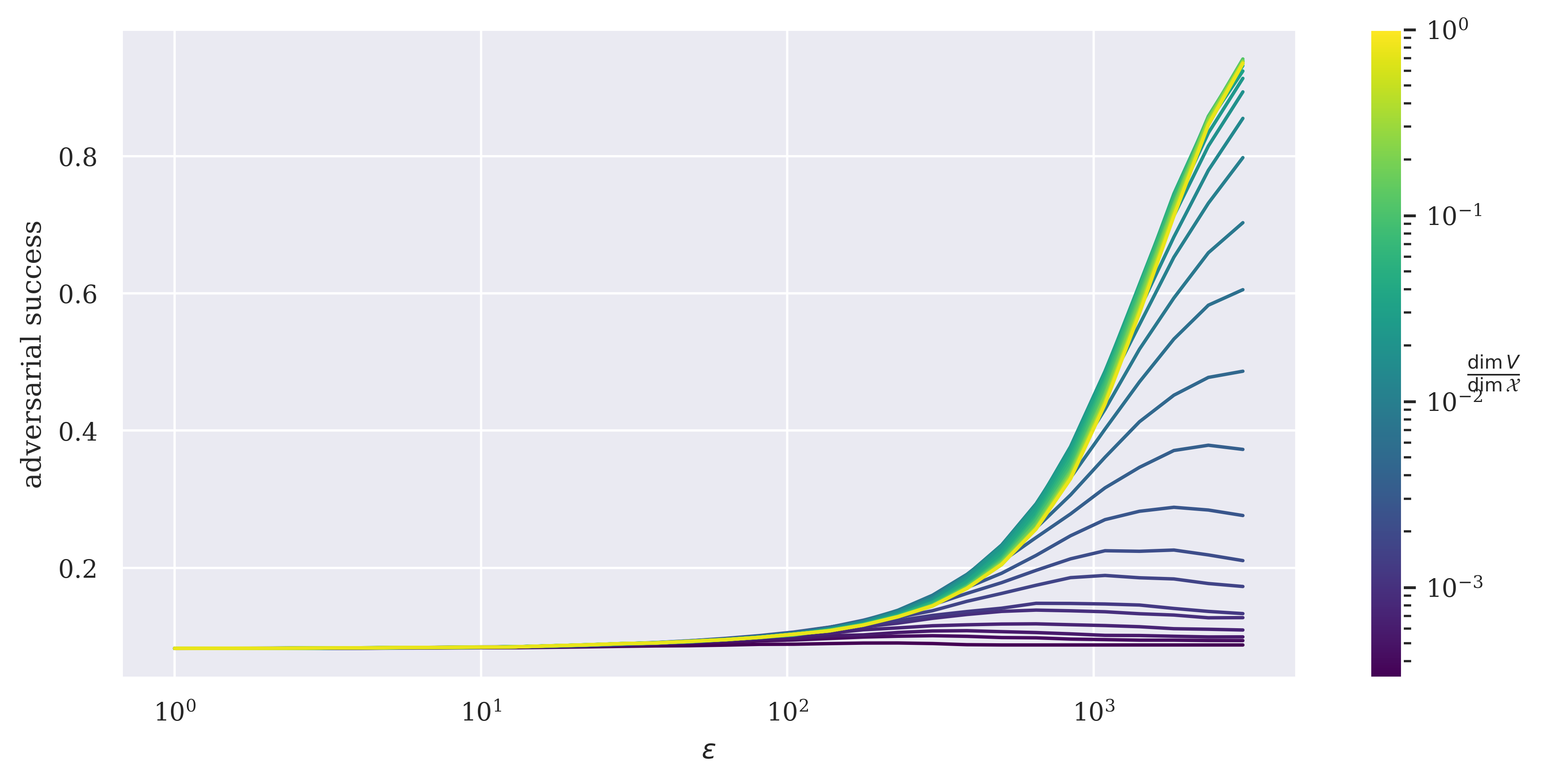
(a)

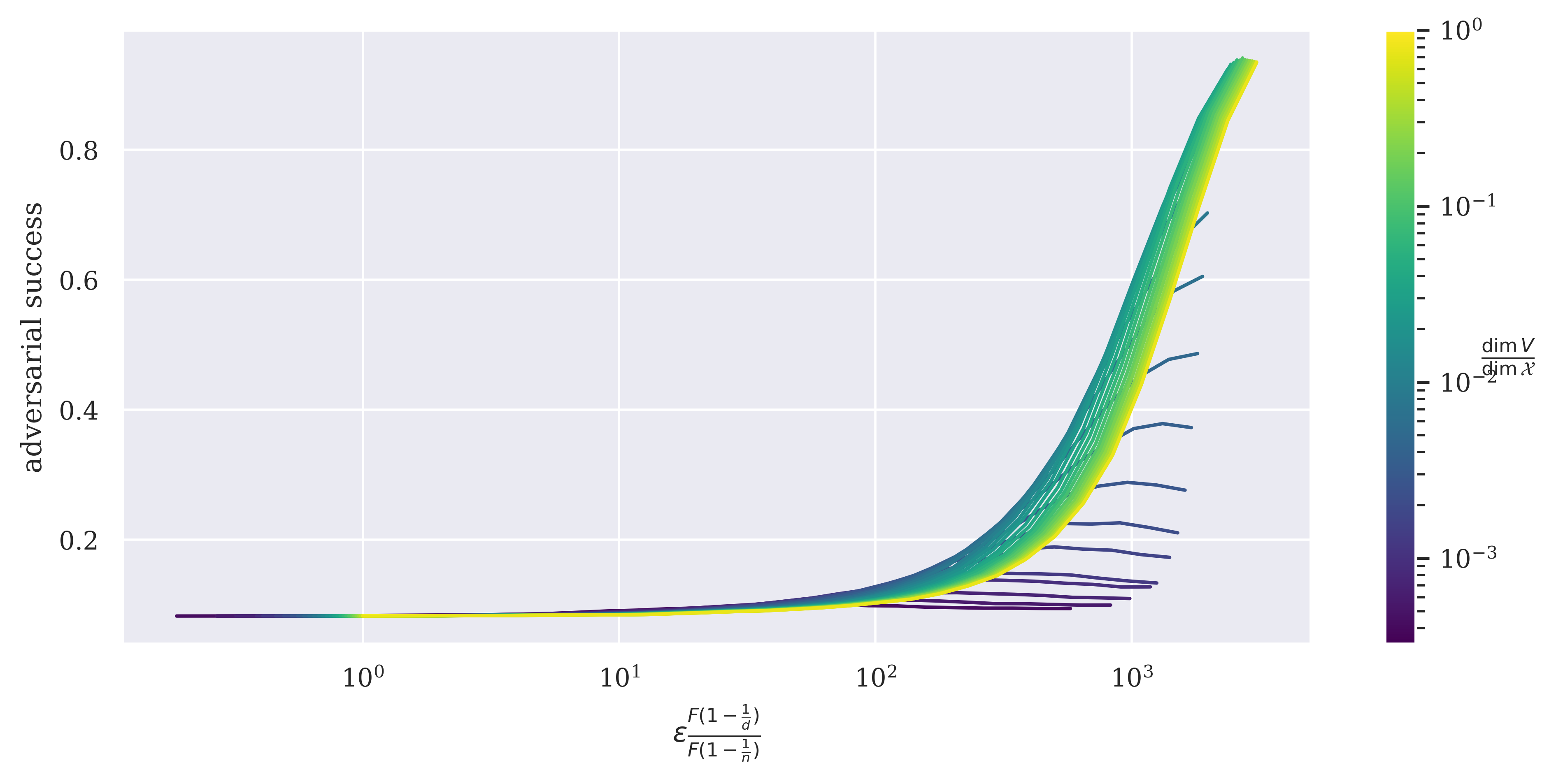
(b)

Figure 9: Plot for experiments analogous to those found in Figure 4 but run with a ResNet9 trained and evaluated on CIFAR10.

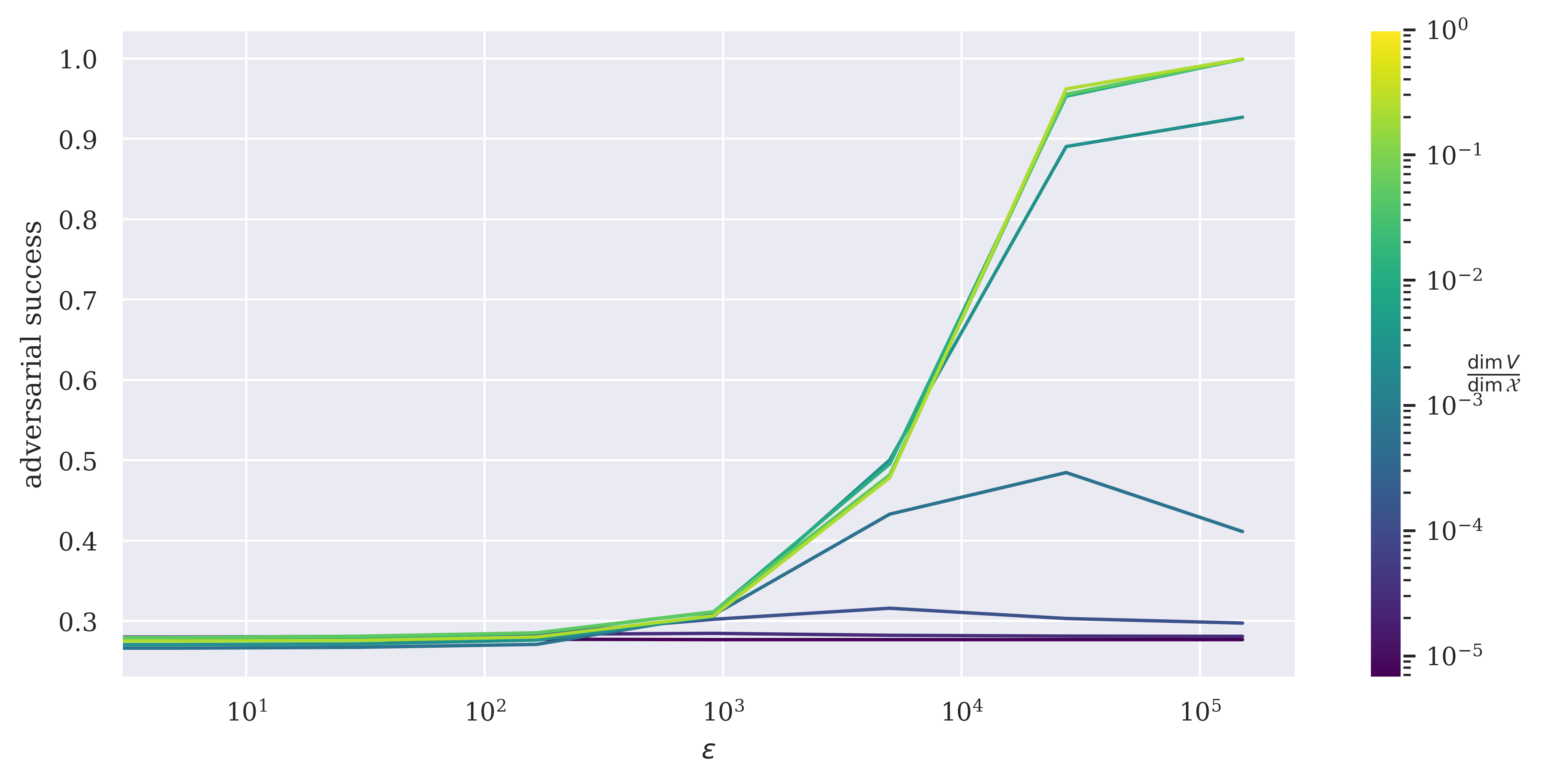
(a)

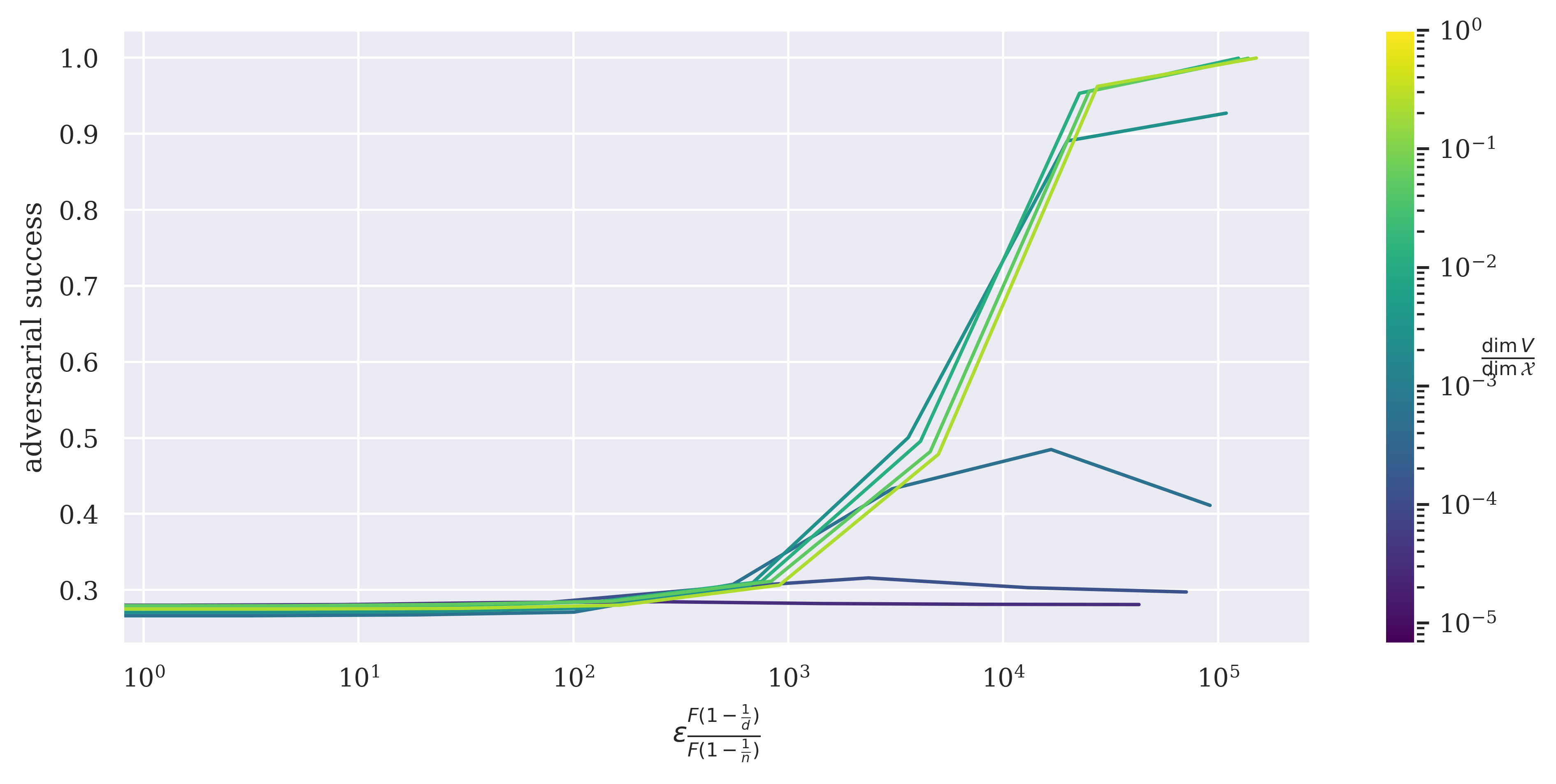
(b)

Figure 10: Plot for experiments analogous to those found in Fig. 4 but run with a ResNet50 trained and evaluated on ImageNet.

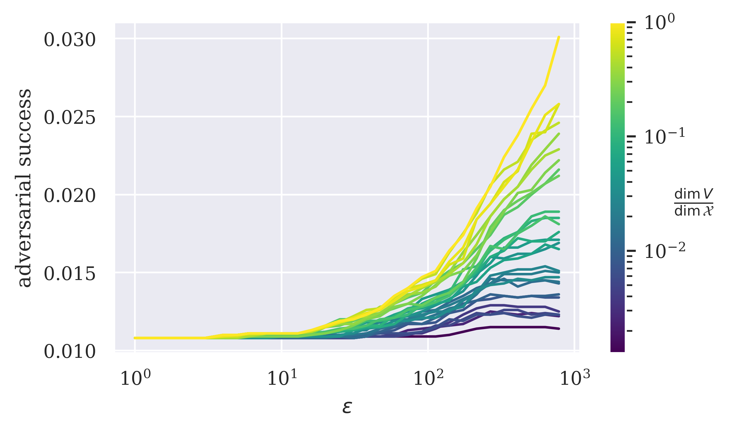
(a)

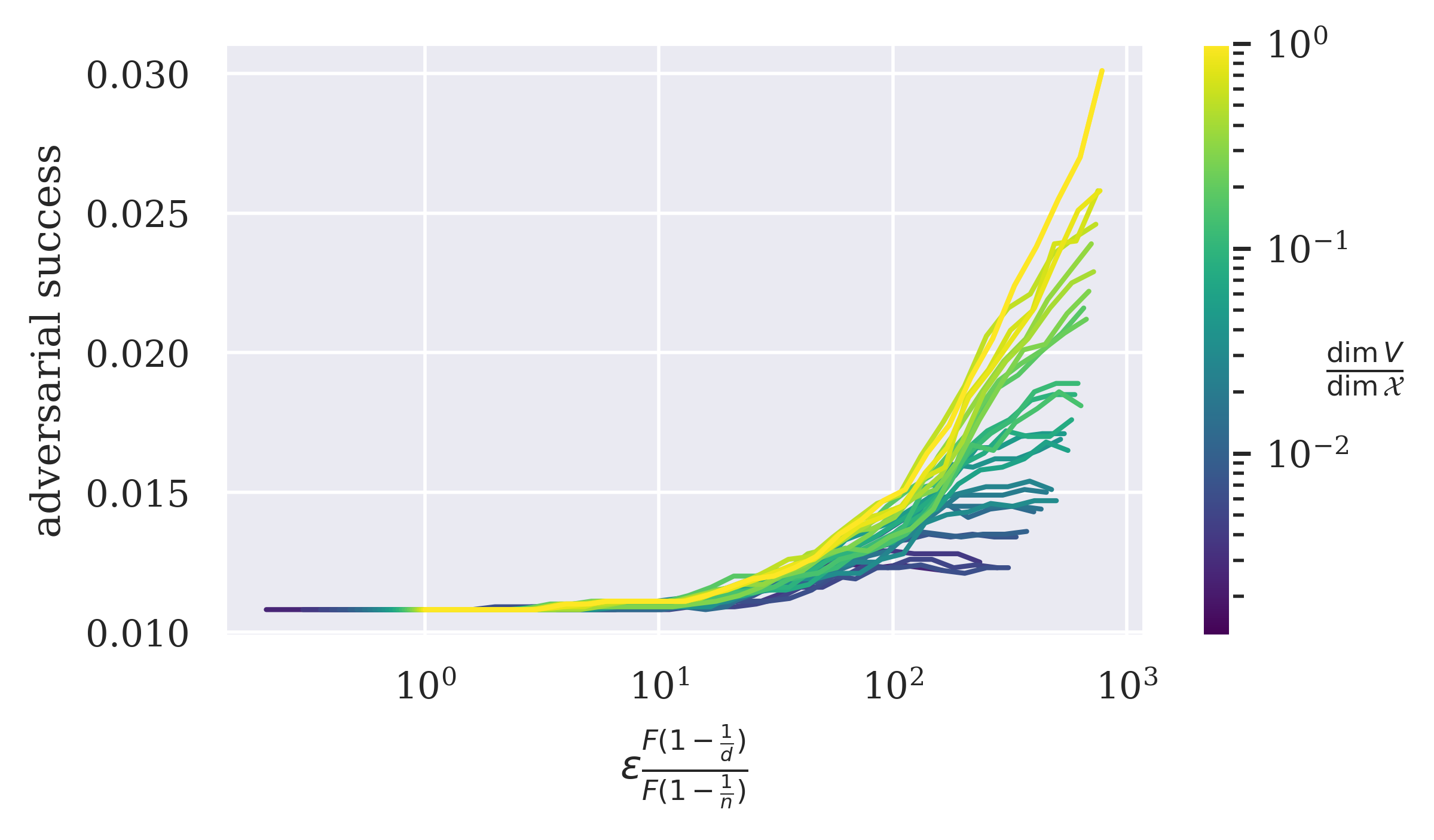
(b)

Figure 11: Plot for experiments analogous to those found in Figure 4, the only difference being that we use the FGSM step of Eq. B.16.

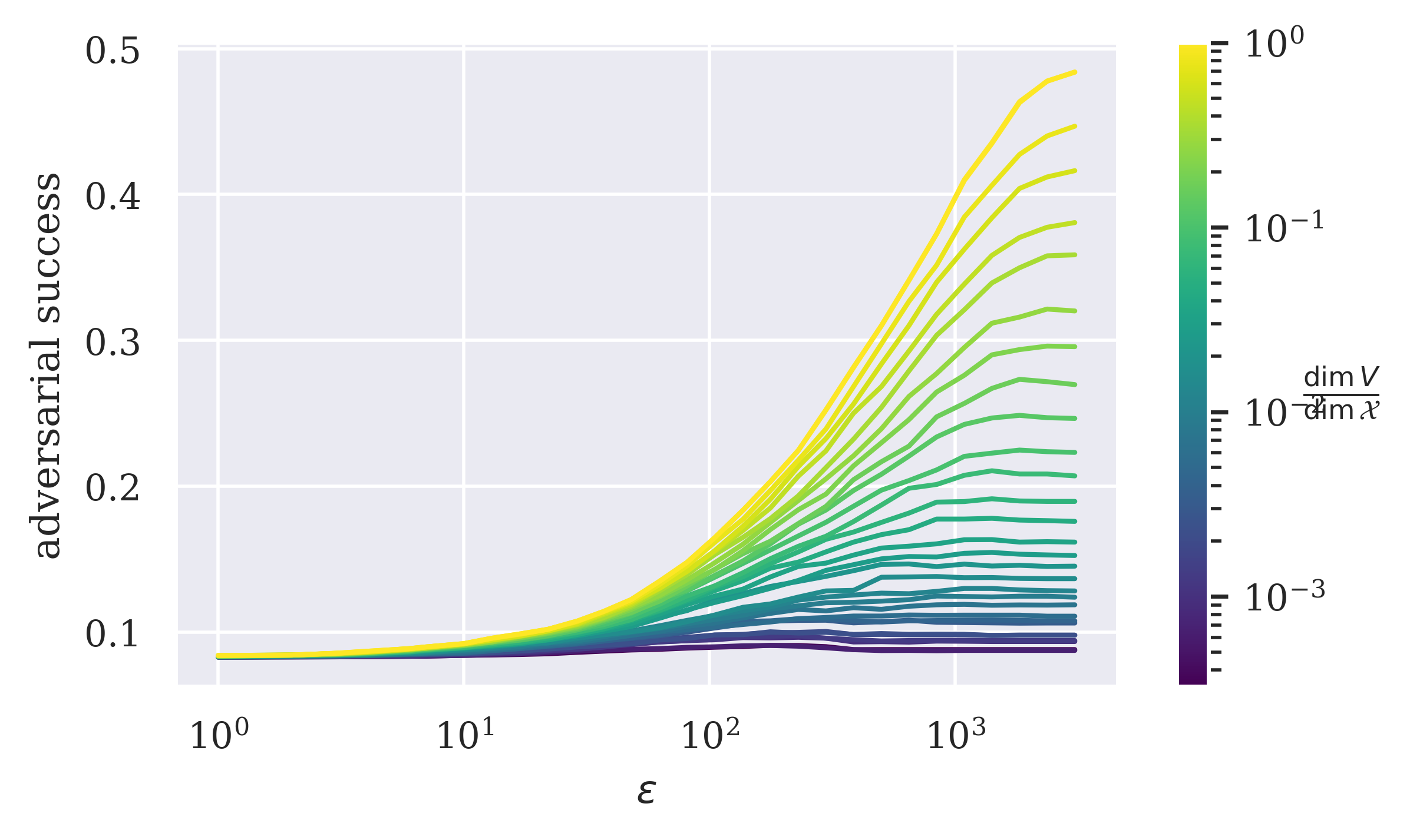
(a)

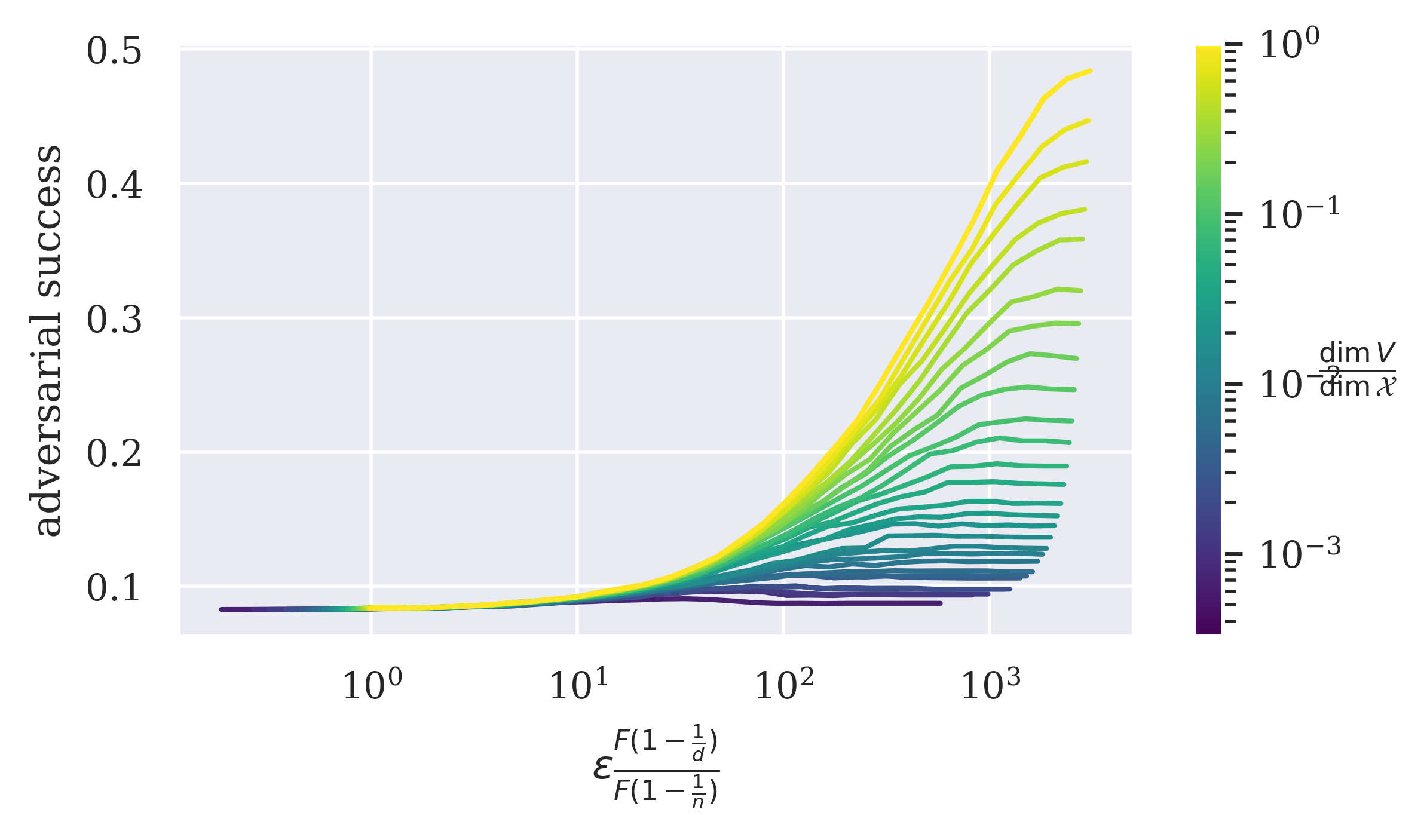
(b)

Figure 12: Plot for experiments analogous to those found in Figure 4 but run with a ResNet9 trained and evaluated on CIFAR10, using the FGSM step of Eq. B.16.

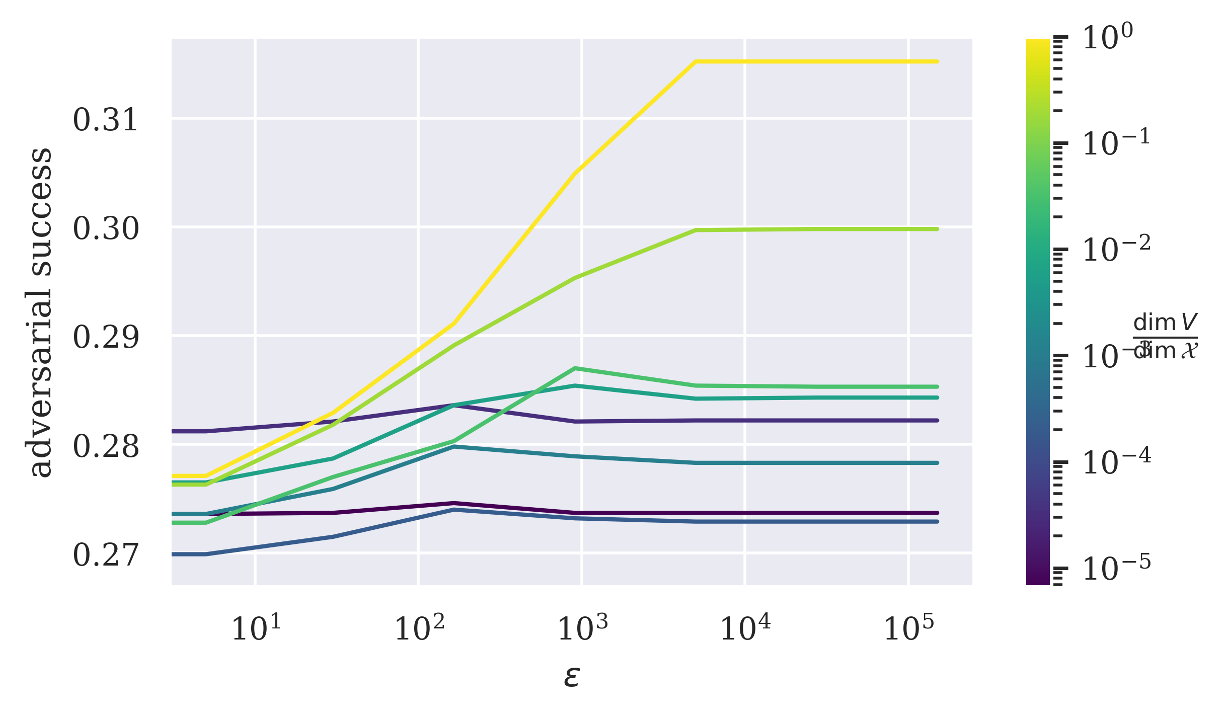
(a)

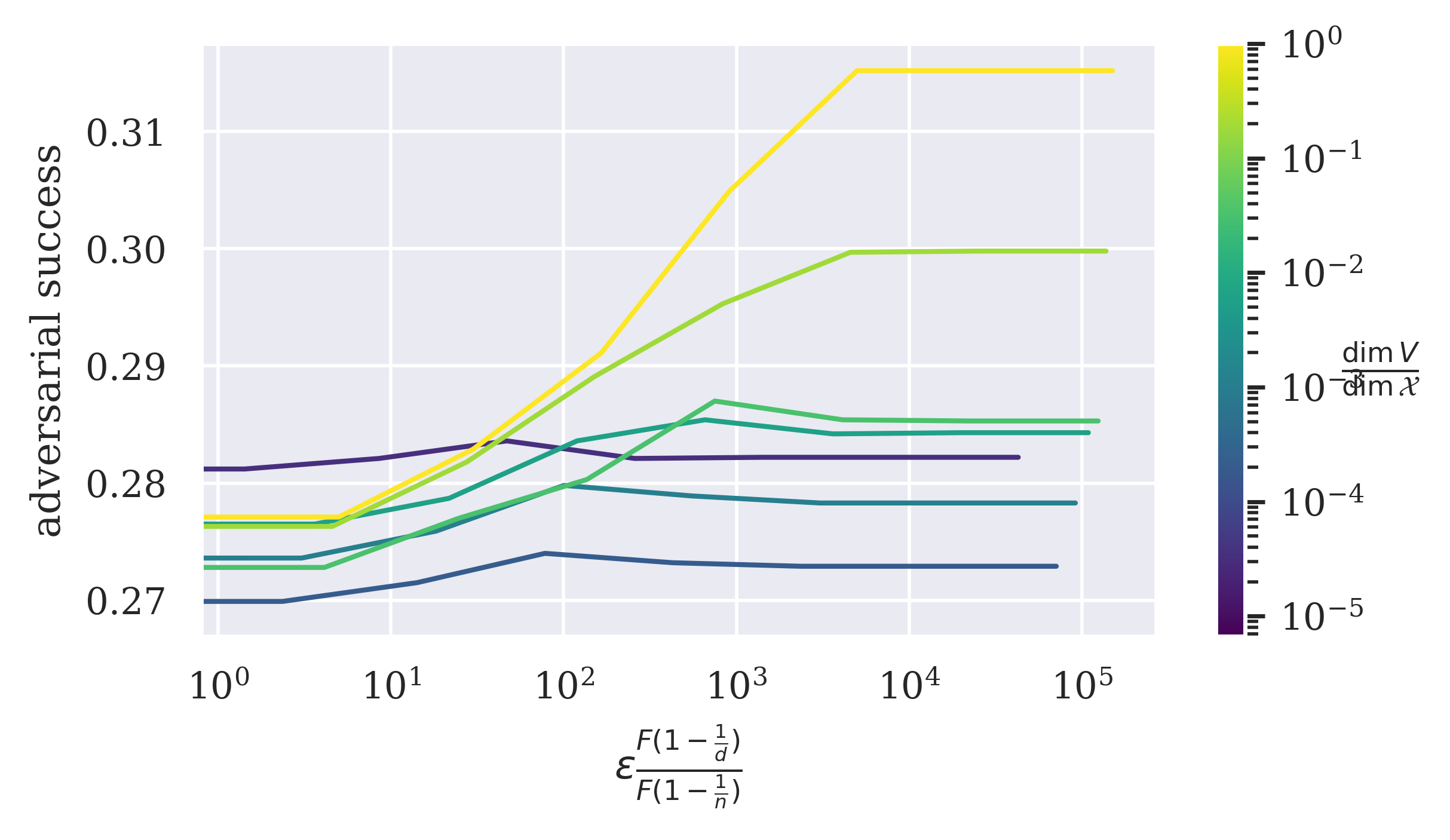
(b)

Figure 13: Plot for experiments analogous to those found in Fig. 4 but run with a ResNet50 trained and evaluated on ImageNet, using the FGSM step of Eq. B.16.

References

- [1] Francis Bach, Rodolphe Jenatton, Julien Mairal, and Guillaume Obozinski. Optimization with Sparsity-Inducing Penalties, Nov. 2011.
- [2] R. R. Bahadur. A Note on Quantiles in Large Samples. The Annals of Mathematical Statistics, 37(3):577–580, June 1966.
- [3] Peter Bartlett, Sebastien Bubeck, and Yeshwanth Cherapanamjeri. Adversarial Examples in Multi-Layer Random ReLU Networks. In Advances in Neural Information Processing Systems, volume 34, pages 9241–9252. Curran Associates, Inc., 2021.
- [4] Sebastien Bubeck, Yeshwanth Cherapanamjeri, Gauthier Gidel, and Remi Tachet des Combes. A single gradient step finds adversarial examples on random two-layers neural networks. In Advances in Neural Information Processing Systems, volume 34, pages 10081–10091. Curran Associates, Inc., 2021.
- [5] Nandish Chattopadhyay, Anupam Chattopadhyay, Sourav Sen Gupta, and Michael Kasper. Curse of dimensionality in adversarial examples. In 2019 International Joint Conference on Neural Networks (IJCNN), pages 1–8, 2019.
- [6] Ekin D. Cubuk, Barret Zoph, Samuel S. Schoenholz, and Quoc V. Le. Intriguing Properties of Adversarial Examples, Nov. 2017.
- [7] J. Deng, W. Dong, R. Socher, L.-J. Li, K. Li, and L. Fei-Fei. ImageNet: A large-scale hierarchical image database. In CVPR09, 2009.
- [8] Elvis Dohmatob, Chuan Guo, and Morgane Goibert. Origins of low-dimensional adversarial perturbations, 2022.
- [9] Alhussein Fawzi, Omar Fawzi, and Pascal Frossard. Analysis of classifiers’ robustness to adversarial perturbations. Mach. Learn., 107(3):481–508, 2018.
- [10] Alhussein Fawzi, Seyed-Mohsen Moosavi-Dezfooli, and Pascal Frossard. Robustness of classifiers: from adversarial to random noise. In D. Lee, M. Sugiyama, U. Luxburg, I. Guyon, and R. Garnett, editors, Advances in Neural Information Processing Systems, volume 29. Curran Associates, Inc., 2016.
- [11] Jean-Yves Franceschi, Alhussein Fawzi, and Omar Fawzi. Robustness of classifiers to uniform and gaussian noise. In Amos Storkey and Fernando Perez-Cruz, editors, Proceedings of the Twenty-First International Conference on Artificial Intelligence and Statistics, volume 84 of Proceedings of Machine Learning Research, pages 1280–1288. PMLR, 09–11 Apr 2018.
- [12] Justin Gilmer, Ryan P. Adams, Ian Goodfellow, David Andersen, and George E. Dahl. Motivating the Rules of the Game for Adversarial Example Research, July 2018.
- [13] Justin Gilmer and Dan Hendrycks. A Discussion of ’Adversarial Examples Are Not Bugs, They Are Features’: Adversarial Example Researchers Need to Expand What is Meant by ’Robustness’. Distill, 4(8):e00019.1, Aug. 2019.
- [14] Ian Goodfellow, Jonathon Shlens, and Christian Szegedy. Explaining and harnessing adversarial examples. In International Conference on Learning Representations, 2015.
- [15] Chuan Guo, Jared S. Frank, and Kilian Q. Weinberger. Low Frequency Adversarial Perturbation. In UAI.
- [16] Kaiming He, X. Zhang, Shaoqing Ren, and Jian Sun. Deep residual learning for image recognition. 2016 IEEE Conference on Computer Vision and Pattern Recognition (CVPR), pages 770–778, 2016.
- [17] Jason Jo and Yoshua Bengio. Measuring the tendency of cnns to learn surface statistical regularities. ArXiv, abs/1711.11561, 2017.
- [18] Marc Khoury and Dylan Hadfield-Menell. On the geometry of adversarial examples. 2018.
- [19] Alex Krizhevsky. Learning multiple layers of features from tiny images. 2009.
- [20] Aditya Kuppa, Slawomir Grzonkowski, Muhammad Rizwan Asghar, and Nhien-An Le-Khac. Black box attacks on deep anomaly detectors. In Proceedings of the 14th international conference on availability, reliability and security, pages 1–10, 2019.
- [21] Cassidy Laidlaw and Soheil Feizi. Functional adversarial attacks. In Hanna M. Wallach, Hugo Larochelle, Alina Beygelzimer, Florence d’Alché-Buc, Emily B. Fox, and Roman Garnett, editors, Advances in Neural Information Processing Systems 32: Annual Conference on Neural Information Processing Systems 2019, NeurIPS 2019, December 8-14, 2019, Vancouver, BC, Canada, pages 10408–10418, 2019.
- [22] Yann LeCun, Corinna Cortes, and CJ Burges. Mnist handwritten digit database. ATT Labs [Online]. Available: http://yann.lecun.com/exdb/mnist, 2, 1998.
- [23] Aleksander Madry, Aleksandar Makelov, Ludwig Schmidt, Dimitris Tsipras, and Adrian Vladu. Towards deep learning models resistant to adversarial attacks. In International Conference on Learning Representations, 2018.
- [24] Sébastien Marcel and Yann Rodriguez. Torchvision the machine-vision package of torch. In Proceedings of the 18th ACM International Conference on Multimedia, MM ’10, page 1485–1488, New York, NY, USA, 2010. Association for Computing Machinery.
- [25] Natalie Maus, Patrick Chao, Eric Wong, and Jacob Gardner. Adversarial prompting for black box foundation models. arXiv preprint arXiv:2302.04237, 2023.
- [26] Seyed-Mohsen Moosavi-Dezfooli, Alhussein Fawzi, and Pascal Frossard. Deepfool: A simple and accurate method to fool deep neural networks. 2016 IEEE Conference on Computer Vision and Pattern Recognition (CVPR), pages 2574–2582, 2016.
- [27] Adam Paszke, Sam Gross, Francisco Massa, Adam Lerer, James Bradbury, Gregory Chanan, Trevor Killeen, Zeming Lin, Natalia Gimelshein, Luca Antiga, Alban Desmaison, Andreas Kopf, Edward Yang, Zachary DeVito, Martin Raison, Alykhan Tejani, Sasank Chilamkurthy, Benoit Steiner, Lu Fang, Junjie Bai, and Soumith Chintala. Pytorch: An imperative style, high-performance deep learning library. In H. Wallach, H. Larochelle, A. Beygelzimer, F. d'Alché-Buc, E. Fox, and R. Garnett, editors, Advances in Neural Information Processing Systems 32, pages 8024–8035. Curran Associates, Inc., 2019.
- [28] Nasim Rahaman, Aristide Baratin, Devansh Arpit, Felix Draxler, Min Lin, Fred Hamprecht, Yoshua Bengio, and Aaron Courville. On the spectral bias of neural networks. In Kamalika Chaudhuri and Ruslan Salakhutdinov, editors, Proceedings of the 36th International Conference on Machine Learning, volume 97 of Proceedings of Machine Learning Research, pages 5301–5310. PMLR, 09–15 Jun 2019.
- [29] Ali Shafahi, W. Ronny Huang, Christoph Studer, Soheil Feizi, and Tom Goldstein. Are adversarial examples inevitable? In International Conference on Learning Representations, 2019.
- [30] Yash Sharma, G. Ding, and Marcus A. Brubaker. On the Effectiveness of Low Frequency Perturbations.
- [31] Carl-Johann Simon-Gabriel, Yann Ollivier, Leon Bottou, Bernhard Schölkopf, and David Lopez-Paz. First-order adversarial vulnerability of neural networks and input dimension. In Kamalika Chaudhuri and Ruslan Salakhutdinov, editors, Proceedings of the 36th International Conference on Machine Learning, volume 97 of Proceedings of Machine Learning Research, pages 5809–5817. PMLR, 09–15 Jun 2019.
- [32] David Stutz, Matthias Hein, and Bernt Schiele. Disentangling adversarial robustness and generalization. 2019.
- [33] Christian Szegedy, Wojciech Zaremba, Ilya Sutskever, Joan Bruna, Dumitru Erhan, Ian Goodfellow, and Rob Fergus. Intriguing properties of neural networks. In International Conference on Learning Representations, 2014.
- [34] The Mosaic ML Team. composer. https://github.com/mosaicml/composer/, 2021.
- [35] Florian Tramèr, Nicolas Papernot, Ian Goodfellow, Dan Boneh, and Patrick McDaniel. The space of transferable adversarial examples. arXiv preprint arXiv:1704.03453, 2017.
- [36] Pauli Virtanen, Ralf Gommers, Travis E. Oliphant, Matt Haberland, Tyler Reddy, David Cournapeau, Evgeni Burovski, Pearu Peterson, Warren Weckesser, Jonathan Bright, Stéfan J. van der Walt, Matthew Brett, Joshua Wilson, K. Jarrod Millman, Nikolay Mayorov, Andrew R. J. Nelson, Eric Jones, Robert Kern, Eric Larson, C J Carey, İlhan Polat, Yu Feng, Eric W. Moore, Jake VanderPlas, Denis Laxalde, Josef Perktold, Robert Cimrman, Ian Henriksen, E. A. Quintero, Charles R. Harris, Anne M. Archibald, Antônio H. Ribeiro, Fabian Pedregosa, Paul van Mulbregt, and SciPy 1.0 Contributors. SciPy 1.0: Fundamental Algorithms for Scientific Computing in Python. Nature Methods, 17:261–272, 2020.
- [37] Cihang Xie, Jianyu Wang, Zhishuai Zhang, Yuyin Zhou, Lingxi Xie, and Alan Yuille. Adversarial examples for semantic segmentation and object detection. In Proceedings of the IEEE international conference on computer vision, pages 1369–1378, 2017.
- [38] Dong Yin, Raphael Gontijo Lopes, Jon Shlens, Ekin Dogus Cubuk, and Justin Gilmer. A fourier perspective on model robustness in computer vision. In NeurIPS, pages 13255–13265, 2019.
- [39] Zhengyu Zhao, Zhuoran Liu, and Martha A. Larson. Adversarial color enhancement: Generating unrestricted adversarial images by optimizing a color filter. In BMVC, 2020.