Onsager coefficients in a coupled-transport model displaying a condensation transition

Abstract

We study nonequilibrium steady states of a one-dimensional stochastic model, originally introduced as an approximation of the Discrete Nonlinear Schrödinger equation. This model is characterized by two conserved quantities, namely mass and energy; it displays a “normal”, homogeneous phase, separated by a condensed (negative-temperature) phase, where a macroscopic fraction of energy is localized on a single lattice site. When steadily maintained out of equilibrium by external reservoirs, the system exhibits coupled transport herein studied within the framework of linear response theory. We find that the Onsager coefficients satisfy an exact scaling relationship, which allows reducing their dependence on the thermodynamic variables to that on the energy density for unitary mass density. We also determine the structure of the nonequilibrium steady states in proximity of the critical line, proving the existence of paths which partially enter the condensed region. This phenomenon is a consequence of the Joule effect: the temperature increase induced by the mass current is so strong as to drive the system to negative temperatures. Finally, since the model attains a diverging temperature at finite energy, in such a limit the energy-mass conversion efficiency reaches the ideal Carnot value.

Keywords: Transport processes (theory); Onsager coefficients; Real-space condensation

1 Introduction

The characterization of non-equilibrium steady states (NESS) is an important research area, as Nature is plenty of systems that steadily exchange physical quantities (e.g., energy, mass) with the surrounding environment. In this area, linear response theory represents a cornerstone; it allows, in fact, expressing transport coefficients in terms of equilibrium fluctuations, under the condition of weak currents. The treatment of systems far from equilibrium is still a challenge although some progress has been recently made thanks to the application of large-deviation theories [1, 2].

Anyway, even in the realm of regimes close to equilibrium, there are nontrivial open questions. For instance, in low-dimensional systems, the long-range correlations which characterize NESS may be so important as to induce anomalous (diverging) conductivity [3, 4, 5]. In this context, additional tools based on fluctuating hydrodynamics [6] are required to account for the resulting scenario, and yet a few challenging exceptions still need be explained (see the summary in [7]).

Another area concerns coupled transport phenomena in systems where two or more quantities are simultaneously transported. For instance, identifying the conditions of an optimal thermoelectric conversion is very important because of potential applications for energy production and storage [8]. A general answer will likely require substantial progress on the basic mechanisms; for instance, in Ref. [9] it has been discovered that combining coupled transport with anomalous transport may be a way to increase the efficiency.

Altogether, the analysis of simple models is potentially very useful because they allow both for the development of analytical treatments and for the performance of detailed numerical investigations. In fact, the one-dimensional setup, where a chain of point-like elements is put in contact with two different reservoirs at its ends, has attracted much attention [3]. The most paradigmatic example is perhaps the asymmetric simple exclusion process (ASEP) [10], introduced to describe the transport of particles through a channel, which revealed quite useful to describe molecular motors [11]. Another celebrated example is the exactly solvable model proposed in 1982 by Kipnis, Marchioro and Presutti to describe energy diffusion in one-dimensional systems [12]. Here, the presence of long-range correlations is explicitly accounted for and the invariant non-equilibrium measure is exactly known. Linear oscillators accompanied by random elastic collisions are another enlightening model, where the stochastic collisions mimic nonlinearities, destroying the integrability of the harmonic chain. This model is indeed an archetypical system displaying anomalous heat conductivity [13].

The above methodology turns out to be useful also in the context of coupled transport problems, as very little is known on the thermodiffusive behavior of interacting systems from the statistical mechanical point of view [8, 14, 15].

In this paper, we focus on a stochastic interacting system, which, roughly speaking, extends the model proposed and solved in Ref. [12]. Here, there is a single set of microscopic-state variables $c_{i}$, and two positive-defined conserved quantities, formally identifiable with total mass and energy. This model can be seen as a simplified stochastic version of the Discrete NonLinear Schrödinger (DNLS) equation, which arises ubiquitously in nonlinear physics and displays important applications in cold-atoms physics and nonlinear optics [16]. In this perspective, the variable $c_{i}$ has the physical meaning of the local norm of the DNLS wavefunction on lattice site (see [17, 18, 19, 20, 21] for related studies and details on the derivation).

The model was originally introduced to investigate the spontaneous onset of energy localization in the DNLS dynamics [17], but it has become a typical example of constraint-driven condensation [22, 23, 24]. In fact, depending on the densities of the two conserved quantities, a finite fraction of energy may eventually condense on a single site, a regime characterized by a negative absolute temperature [25, 26]. At equilibrium, a critical line of infinite-temperature states separates the condensed region from a homogeneous one displaying standard equipartition [27]. In this model, the energy localization mechanism is the direct consequence of the existence of two conservation laws along with the positivity constraint, $c_{i}\geq 0$. For this reason, we refer to it as C2C (condensation with two conserved quantities); see the next section for a more precise definition.

When a C2C chain is attached to two different reservoirs at its boundaries, the corresponding NESS can be visualized as a path in the thermodynamic plane (characterized by either mass and energy density in the microcanonical plane, or chemical potential and temperature in the grand canonical plane). Recently, it has been found that such paths may spontaneously enter the condensed region even when the extrema lie in the homogeneous region [28]. In practice, enegy can robustly localize within an internal portion of the chain, while the boundaries of the system behave smoothly and display standard thermal fluctuations. These examples reveal a novel type of condensation that takes place exclusively in out-of-equilibrium conditions and in the presence of coupled transport.

The accessibility of such unusual nonequilibrium states is manifestly a relevant research subject in the context of irreversible thermodynamics. Here, we thoroughly explore the NESS emerging in the C2C model with the help of linear response theory, devoting a special attention to the behavior close to the critical line. An exact scaling analysis shows that the two-parameter dependence of the thermodynamic states can be reduced to the dependence on a single variable. This includes the coefficients of the Onsager matrix, whose behavior is crucial to reconstruct NESS paths.

We find that the Onsager coefficients are well-defined and finite along the whole critical line of the model, thus making it possible a novel and potentially useful kind of “infinite-temperature transport”. We derive perturbative expressions of the corresponding paths and, more important, we identify the class of paths which are due to enter the condensed phase. Qualitatively, this phenomenon can be seen as an extreme version of a Joule effect: the mass current induced by the external reservoirs heats up the interior of the system forcing it to go beyond the infinite-temperature line, i.e. to condense. Moreover, we show that in proximity to the critical line, the thermodiffusive conversion performance reaches its maximum value (as expressed in terms of the Carnot efficiency).

We are able to show that nonequilibrium correlations arising in NESSs play an important role in the high-temperature limit, thus making the C2C transport substantially different from that of noninteracting dilute gases. Approximate analytic expressions of the Onsager transport coefficients are obtained in the opposite regime of small-temperatures, where spatial correlations are negligible. There, we also find that the Seebeck coefficient, which quantifies the coupling between mass and energy currents, vanishes rather rapidly when the ground state is approached.

The paper is organized as follows. In Sec. 2 we introduce the model, its equilibrium and out-of-equilibrium properties, and show that (local) equilibrium properties depend on one parameter only: a suitable combination of mass and energy in the microcanonical ensemble; a combination of temperature and chemical potential in the grand canonical ensemble. In Sec. 3 we introduce and determine the Onsager coefficients. Because of scaling properties, it is sufficient to determine them for a unitary value of the mass density. In Sec. 4 we evaluate spatial correlations and discuss their increasing importance when temperature grows. In Sec. 5 we estimate the steady-state paths in proximity of the critical line and determine the condition for them to enter the negative-temperature region. In Sec. 6 we discuss the Seebeck coefficient and the conversion efficiency. Finally, in Sec. 7 we provide some concluding remarks. A contains some technical details, and a slightly different model is presented in B.

2 The model and its equilibrium and out-of-equilibrium properties

The C2C model is defined on a lattice whose nodes $i$ host a non negative quantity $c_{i}\geq 0$, here called (local) mass. Its square is called (local) energy, $\epsilon_{i}\equiv c_{i}^{2}$. Both the total mass $(A=\sum_{i}c_{i})$ and the total energy $(H=\sum_{i}\epsilon_{i})$ are conserved and the model is microcanonically defined through the mass density $a=A/N$ and the energy density $h=H/N$, where $N$ is the total number of sites.

The equilibrium properties are well understood [22, 25, 27, 28]. The system has a homogeneous phase for $a^{2}\leq h\leq 2a^{2}$ and a condensed/localized phase for $h>2a^{2}$, characterized in the thermodynamic limit by a single site hosting a finite fraction of the whole energy, equal to $(h-2a^{2})N$. Finite-size effects provide an interesting and unexpected scenario close to the critical line, $h_{c}=2a^{2}$ [24]. When $h$ varies between the ground state $h=a^{2}$ and the upper value of the homogeneous phase, $h=h_{c}$, the temperature varies between $T=0$ and $T=+\infty$. In the localized region, the temperature is constant and equal to $T=+\infty$ but subleading terms in the entropy (i.e., non extensive terms) show that finite-size systems are characterized by a negative temperature when $h_{c}<h<h_{c}+\xi(N)$, where $\xi(N)\simeq 11.05/N^{1/3}$, see Ref. [25]. In such a region the system is effectively delocalized [27].

The grand canonical description is well defined in the homogeneous phase only, $h\leq h_{c}$, where there is ensemble equivalence [25]. The grand canonical partition function reads

$$Z(\beta,\mu)=\left[\int_{0}^{+\infty}dc\,e^{-\beta(c^{2}-\mu c)}\right]^{N}\,.$$ (1)

As already detailed in Ref. [28], the inverse temperature $\beta=1/T$ and the chemical potential $\mu$ are related to the mass density $a$ and to the energy density $h$ through the relations

$$a = \frac{\mu}{2}+\frac{1}{\sqrt{\pi\beta}}\frac{e^{-\beta\mu^{2}/4}}{1+\mbox{erf}\left(\frac{\sqrt{\beta}\mu}{2}\right)},$$ (2)

$$h = \frac{1}{2\beta}+\frac{1}{2}a\mu.$$ (3)

Eqs. (2,3) provide a mapping from grand canonical to microcanonical quantities. While numerical simulations allow for a direct extraction of $(a,h)$, the Onsager coefficients are better expressed in terms of grand canonical quantities. It is therefore useful to invert the above mapping. We start introducing

$$m=\mu\beta.$$ (4)

as this also helps unveiling a general scaling dependence. If we further introduce the auxiliary variable

$$z=\frac{m}{\sqrt{\beta}},$$ (5)

relations (2-3) can be rewritten as

$$a = \frac{1}{m}\left[\frac{z^{2}}{2}+\frac{z}{\sqrt{\pi}}\frac{\mathrm{e}^{-z^{2}/4}}{1+\mathrm{erf}(z/2)}\right]\equiv\frac{\tilde{m}(z)}{m}$$ (6)

$$h = a^{2}\cdot\frac{z^{2}}{2}\left(\frac{1}{\tilde{m}^{2}(z)}+\frac{1}{\tilde{m}(z)}\right)\equiv a^{2}{\tilde{h}}(z).$$ (7)

Eq. (7) demonstrates that the specific energy $\tilde{h}\equiv h/a^{2}$ is a function of $z$ only. Indeed, the invariance of the model under a uniform rescaling of the $c_{i}$’s implies that the mass density $a$ is essentially a unit of measure and that global and local equilibrium properties depend only on $\tilde{h}$, or equivalently on $z$.

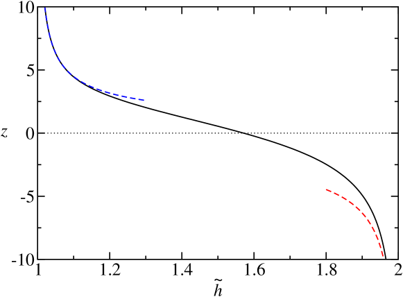
Figure 1: The dependence of $z$ on the effective energy $\tilde{h}$ as determined by Eq. (7). As $\tilde{h}$ varies from $1$ to $2$, the temperature increases from $0$ to $+\infty$, and $z=\mu\sqrt{\beta}$ varies between $+\infty$ and $-\infty$. The change of sign of $z$ corresponds to a change of sign of the chemical potential. The dashed lines represent the analytical approximations of Eq. (10), valid for vanishing and diverging temperature.

In fact, $\tilde{h}(z)$ plays a crucial role to understand the relastionship between the microcanonical and grand canonical representention. First of all, as shown in Fig. 1, this function is one-to-one and thus perfectly invertible. In the same figure we plot also the limiting behavior determined via a perturbative analysis carried out in A,

$$z\simeq\left\{\begin{array}[]{lcc}\displaystyle\sqrt{2/(\tilde{h}-1)}&&\tilde{h}\to 1\\ \displaystyle-2/\sqrt{2-\tilde{h}}&&\tilde{h}\to 2.\end{array}\right.$$ (10)

In practice, from the $a$ and $h$ values, the specific energy $\tilde{h}$ is first obtained and thereby the corresponding $z$ value. Afterwards $m$ can be obtained as $\tilde{m}(z)/a$ and finally $\beta=m^{2}/z^{2}$. A schematic representation of the mapping is presented in Fig. 2.

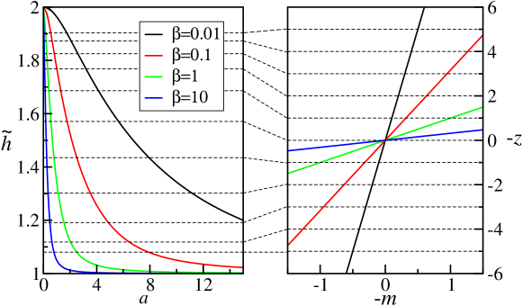
Figure 2: Isothermal lines $\beta=$ const in the $(a,\tilde{h})$ space (left panel) and in the $(m,z)$ one (right panel). Dashed lines are examples of curves at constant $\tilde{h}$ which are mapped to horizontal lines $z=$ const by Eqs. (6-7).

For $\tilde{h}\to 1$ (zero temperature), the chemical potential $\mu$ is finite and positive, while $m$ diverges to infinity; For $\tilde{h}\to 2$ (infinite temperature) $\mu\to-\infty$, while $m$ is finite and negative.

The study of out-of-equilibrium properties requires the definition of some dynamical rule. The C2C dynamics is actually simulated by a Monte Carlo Microcanonical (MMC) algorithm, where the two conservation laws are implemented for randomly selected triplets of neighbouring sites$(i-1,i,i+1)$, so as to satisfy detailed balance [18]. In practice this amounts to pass from $(c_{i-1},c_{i},c_{i+1})$ to $(c^{\prime}_{i-1},c^{\prime}_{i},c^{\prime}_{i+1})$, in such a way that (i) the sum of the three masses and of their squares is conserved and (ii) that the probability of the transition $\{c\}\to\{c^{\prime}\}$ is equal to the probability of the inverse transition, $\{c^{\prime}\}\to\{c\}$. Geometrically, legal configurations of triplet states lie within the intersection between a plane and a sphere in a three-dimensional space, which are representative of mass- and energy conservation, respectively. Since these two constraints define a circle in a three dimensional space, detailed balance is ensured by picking a random angle. Depending on the further constraint posed by the mass positivity, $c^{\prime}_{i}\geq 0$, physically accessible states consist of either a full circle, or the union of three disconnected arcs (see Fig. 3). Here, we have adopted the rule that the new state should be restricted to the same starting arc, but in B we also briefly consider the case when such restriction is removed.

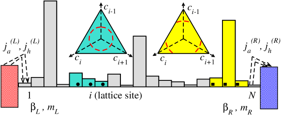
Figure 3: The transport setup: a C2C chain steadily interacts with two reservoirs at its boundaries. Boundary thermal conditions are specified by the couple of values $\beta$ and $m\equiv\beta\mu$. $j_{a}$ and $j_{h}$ represent the mass and the energy current, respectively. A NESS is characterized by equal currents at the boundaries, $j_{a,h}^{L}=j_{a,h}^{R}$. Bulk dynamics is implemented using the MMC algorithm (see text) on random triplets of consecutive sites. Local conservation of energy and mass restricts the available states in the space $(c_{i-1},c_{i},c_{i+1})$ on the intersection between a plane (colored triangles) and a sphere (not shown), restricted to the positive octant $c_{i}\geq 0$. The resulting set of states is either a full circle (left triangle) or a union of three distinct arcs (right triangle): in both cases the intersection is given by the red dashed lines.

Out-of-equilibrium (grand canonical) simulations can be performed by attaching the two lattice ends to thermal reservoirs. Customarily, a Monte Carlo grand canonical heat baths [28] are used. In this paper, we directly impose the exact equilibrium distributions of masses, which allows sampling more efficiently the NESS, especially in proximity of the critical line. In practice we extract at random an integer $k\in[1,N]$. If $k\neq 1,N$ we update the triplet $(k-1,k,k+1)$ as explained here above. If $k=1$ ($k=N$), we extract a random mass $c\geq 0$ according to the grand canonical distribution $P(c)\sim\exp{(-\beta^{(i)}c^{2}+m^{(i)}c)}$ and we assign it to the chosen site. The parameters $\beta^{(i)},m^{(i)}$ define the heat baths attached to the chain ends ($i=L$ for $k=1$ and $i=R$ for $k=N$), see Fig. 3. As usual in Monte Carlo simulations, time is measured in units of Monte Carlo moves divided by the system size $N$.

Suitable definitions of mass and energy fluxes can be employed to measure the rate of exchange of these two quantities from the reservoirs to the chain. For the left boundary, we define

$$j_{a}^{(L)} = \frac{1}{\tau}\sum_{t_{k}<\tau}\delta c_{1}(t_{k})$$

$$j_{h}^{(L)} = \frac{1}{\tau}\sum_{t_{k}<\tau}\delta c_{1}^{2}(t_{k})\,,$$ (11)

where $\delta c_{1}(t_{k})$ and $\delta c_{1}^{2}(t_{k})$ represent respectively the variations of mass and energy on the first lattice site produced by reservoir updates occurring at times $0\leq t_{k}\leq\tau$. An average over a sufficiently long time window $\tau\gg 1$ must be considered. The definitions of $-j_{a}^{(R)}$ and $-j_{h}^{(R)}$ on the right boundary are readily obtained by replacing $c_{1}\rightarrow c_{N}$ in Eqs. (2). According to these definitions, fluxes are positive when they flow from left to right.

When a NESS is attained, the conditions $j_{a}^{(L)}=j_{a}^{(R)}\equiv j_{a}$ and $j_{h}^{(L)}=j_{h}^{(R)}\equiv j_{h}$ hold and stationary spatial profiles of mass and energy are defined respectively as $a_{i}=\langle c_{i}(t)\rangle$ and $h_{i}=\langle c_{i}^{2}(t)\rangle$, where the symbol $\langle\cdot\rangle$ refers to an average over the NESS distribution. Once plotted parametrically in the plane $(a,h)$ or in the plane $(m,\beta)$ (through the mapping in Eqs. (6-7)) the above paths identify a “trajectory” connecting the boundary conditions imposed by the reservoirs.

3 Onsager coefficients

The presence of two conservation laws in the C2C model implies the existence of mass- and energy currents, which are time and site-independent once the system has reached a NESS. In the limit of small thermodynamic forces, local equilibrium sets in and a linear response approach can be adopted. Using the standard formulation in terms of the variables $(m,\beta)$, we can write

$$j_{a} = -L_{aa}m_{y}+L_{ah}\beta_{y}$$ (12)

$$j_{h} = -L_{ha}m_{y}+L_{hh}\beta_{y},$$ (13)

where $L_{uv}$ with $u,v=\{a,h\}$ identify the coefficients of the Onsager matrix [10] and the subscript $y$ denotes a derivative with respect to the continuous spatial variable $y=i/N$.

A first important point worth discussing is that the form of the equilibrium equations Eqs. (6-7) implies a scaling form for the Onsager coefficients. In fact, if $m\to cm$, then $\beta\to c^{2}\beta$ in order to keep constant $z$. Under the same transformation, see Eqs. (6-7), $(a,j_{a})\to(a,j_{a})/c$ and $(h,j_{h})\to(h,j_{h})/c^{2}$. Imposing that Eqs. (12-13) must be invariant under such scale transformation, each term on the RHS of Eq. (12) must rescale as $1/c$ and each term on the RHS of Eq. (13) must rescale as $1/c^{2}$. Using the scaling assumption

$$L_{uv}(m,\beta)=|m|^{\gamma_{uv}}\overline{L}_{uv}(z)$$ (14)

we obtain the following relations for the scaling exponents $\gamma_{uv}$,

$$1+\gamma_{aa}=-1 2+\gamma_{ah}=-1$$

$$1+\gamma_{ha}=-2 2+\gamma_{hh}=-2,$$ (15)

so that

$$L_{aa}(m,\beta) = |m|^{-2}\overline{L}_{aa}(z)$$

$$L_{ah}(m,\beta) = |m|^{-3}\overline{L}_{ah}(z)$$

$$L_{ha}(m,\beta) = |m|^{-3}\overline{L}_{ha}(z)$$

$$L_{hh}(m,\beta) = |m|^{-4}\overline{L}_{hh}(z).$$ (16)

According to Eq. (14), the dependence of the Onsager matrix on the thermodynamic parameters is determined by the one-parameter functions $\overline{L}_{uv}(z)$, with the additional condition $\overline{L}_{ah}(z)=\overline{L}_{ha}(z)$ due to the well known symmetry property of the Onsager coefficients [8, 10]. By recalling that $m=F_{1}(z)/a$ and that $z$ is a function of $\tilde{h}$, Eqs. (14) can be equivalently written in terms of the microcanonical variables $(a,h)$,

$$L_{uv}(a,h)=a^{-\gamma_{uv}}L^{*}_{uv}(\tilde{h})\,,$$ (17)

perhaps preferable, as $a$ is by definition positive.

In order to test the above scaling, we have plotted $L_{uv}a^{\gamma_{uv}}$ as a function of $\tilde{h}$ for different values of $a$, see Fig. 4. Onsager coefficients were computed using Eqs. (12-13) for given values of the thermodynamic forces and inserting the corresponding values of stationary fluxes determined numerically. Since there are four Onsager coefficients (three independent ones) it is necessary to analyze at least two independent paths passing through the same reference point $(m,\beta)$. The agreement between circles $(a=1)$ and diamonds $(a=2)$ confirms the validity of Eq. (17). The curves plotted in Fig. 4 depend smoothly on $\tilde{h}$ and there is no divergence for $\tilde{h}\to 2$. The behavior of Onsager coefficients in proximity of the critical curve will be treated in more detail in Sec. 3.2.

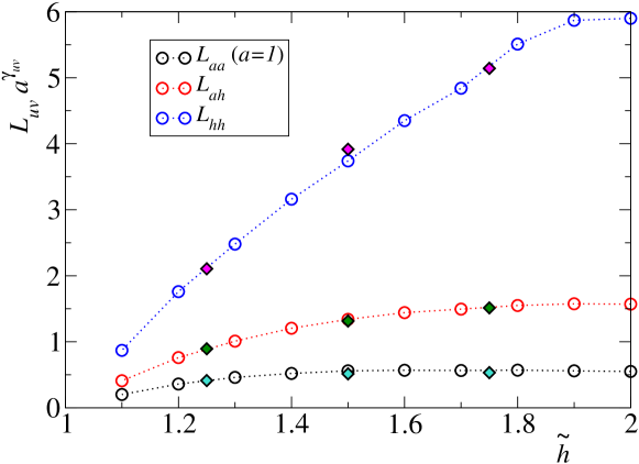
Figure 4: Plots of the Onsager coefficients $L_{aa}$ (lower data), $L_{ah}$ (middle data), and $L_{hh}$ (upper data) as functions of $\tilde{h}$. Circles have been obtained for $a=1$, diamonds for $a=2$. Dotted lines are guides for the eye.

3.1 Low temperature limit

The stochastic move of our MMC algorithm does not allow for a straightforward interpretation of the mass changes. This is because the three-arcs solution, see Fig. 3 and below Eq. (10), depends in a complicated way on the initial triplet. This is no longer the case if the solution is a full circle: in this case, any possible final triplet can be obtained by a random rotation $\theta$, with $0\leq\theta<2\pi$ [18]. Hence, the low$-T$, i.e. $\tilde{h}\to 1$, limit can be treated analytically. In fact, the ground state of the system corresponds to equal masses, $c_{i}\equiv a$, and low$-T$ configurations are characterized by weak spatial fluctuations of the local mass. Therefore, in this limit the intersection between the plane of constant mass and the sphere of constant energy is a full circle. As we are going to argue, this allows to obtain some analytical results.

In formulae, the update $(c_{1},c_{2},c_{3})\rightarrow(c^{\prime}_{1},c^{\prime}_{2},c^{\prime}_{3})$ reads

$$(c^{\prime}_{1},c^{\prime}_{2},c^{\prime}_{3})=R\,(c_{1},c_{2},c_{3})$$ (18)

where $R$ is the rotation matrix around the $(1,1,1)$ direction

$$R=\begin{pmatrix}d&f&s\\ s&d&f\\ f&s&d\end{pmatrix},$$ (19)

with

$$d = \frac{1}{3}+\frac{2}{3}\cos\theta$$

$$f = \frac{1}{3}(1-\cos\theta)-\frac{1}{\sqrt{3}}\sin\theta$$

$$s = \frac{1}{3}(1-\cos\theta)+\frac{1}{\sqrt{3}}\sin\theta.$$ (20)

We now write the mass and energy fluxes as 

$$j_{a}=2\langle\overline{c^{\prime}_{1}}-c_{1}\rangle\quad j_{h}=2\langle\overline{\epsilon^{\prime}_{1}}-\epsilon_{1}\rangle$$ (21)

where the symbol $\overline{\cdots}$ refers to the average over the distribution of $\theta$ for a given initial state $(c_{1},c_{2},c_{3})$, while $\langle\cdots\rangle$ refers to the average over the distribution of the initial triplet, $(c_{1},c_{2},c_{3})$. In the general case, not all $\theta$ angles are allowed because of the constraint $c_{i}^{\prime}\geq 0$. However, if the variance of the three masses is not large, then all $\theta$ are allowed and the average over $\theta$ is trivial .

Let us first consider the expression of the mass flux $j_{a}$. The average of the first of Eq. (21) over the distribution of $\theta$ is easily computed and gives

$$j_{a} = 2\left(\frac{1}{3}\langle c_{1}+c_{2}+c_{3}\rangle-\langle c_{1}\rangle\right)$$ (22)

$$= \frac{2}{3}\langle-2c_{1}+c_{2}+c_{3}\rangle.$$

We now suppose that a mass gradient is present in the triplet:

$$\langle c_{1}\rangle = \langle c_{2}\rangle+\Delta_{m}\equiv a+\Delta_{m}$$

$$\langle c_{3}\rangle = \langle c_{2}\rangle-\Delta_{m}\equiv a-\Delta_{m}.$$ (23)

Inserting these expressions in Eq. (22) we finally obtain

$$j_{a}=-2\Delta_{m}.$$ (24)

Analogous calculations can be performed for the energy flux $j_{h}$. The first average over $\theta$ reads

$$\overline{\epsilon^{\prime}_{1}}-\epsilon_{1} = \overline{[D(\theta)c_{1}+M(\theta)c_{2}+P(\theta)c_{3}]^{2}}-\epsilon_{1}$$ (25)

$$= \frac{1}{3}(-2\epsilon_{1}+\epsilon_{2}+\epsilon_{3}).$$

Then, by assuming an energy gradient

$$\langle\epsilon_{1}\rangle = \langle\epsilon_{2}\rangle+\Delta_{\epsilon}\equiv h+\Delta_{\epsilon}$$

$$\langle\epsilon_{3}\rangle = \langle\epsilon_{2}\rangle-\Delta_{\epsilon}\equiv h-\Delta_{\epsilon}\,,$$ (26)

we obtain

$$j_{h}=-2\Delta_{\epsilon}.$$ (27)

Remarkably, in the low temperature limit both fluxes do not depend on spatial correlations between sites. In a continuum representation we can summarize the above result by writing

$$j_{a} = C_{aa}\,\partial_{y}a+C_{ah}\,\partial_{y}h$$ (28)

$$j_{h} = C_{ah}\,\partial_{y}a+C_{hh}\,\partial_{y}h$$

with

$$C_{aa} = -2$$ (29)

$$C_{ah} = C_{ha}=0$$

$$C_{hh} = -2.$$

Accordingly, in this representation the two currents are decoupled.

In order to determine the proper Onsager coefficients, we need to map Eq. (28) onto Eq. (12). In practice, it is necessary to express the derivatives $\partial_{y}a$ and $\partial_{y}h$ in terms of the thermodynamic forces $\partial_{y}\beta$ and $\partial_{y}m$. In formulae,

$$j_{a} = (C_{aa}\partial_{m}a+C_{ah}\partial_{m}h)\partial_{x}m+(C_{aa}\partial_{\beta}a+C_{ah}\partial_{\beta}h)\partial_{x}\beta$$

$$j_{h} = (C_{ah}\partial_{m}a+C_{hh}\partial_{m}h)\partial_{x}m+(C_{ah}\partial_{\beta}a+C_{hh}\partial_{\beta}h)\partial_{x}\beta$$

By using the relations in Eq. (29), Eq. (3.1) simplifies to

$$j_{a} = -2\partial_{m}a\,\partial_{x}m-2\partial_{\beta}a\,\partial_{x}\beta$$

$$j_{h} = -2\partial_{m}h\,\partial_{x}m-2\partial_{\beta}h\partial_{x}\beta$$

and we obtain

$$L_{aa}=2\partial_{m}a\quad L_{ah}=-2\partial_{\beta}a$$ (30)

$$L_{ha}=2\partial_{m}h\quad L_{hh}=-2\partial_{\beta}h.$$

The derivatives in Eq. (30) are completely determined by the “equation of state” of the model, Eq. (6,7). Moreover, the reciprocity property $L_{ah}=L_{ha}$ is recovered by recalling the standard grand canonical relations $a=\partial_{m}\log Z$ and $h=-\partial_{\beta}\log Z$, where $Z$ is the partition function of the model, see Eq. (1). Indeed, given the regularity of $\log Z$, the equality of off-diagonal coefficients follows from $\partial_{\beta}\partial_{m}\log Z=\partial_{m}\partial_{\beta}\log Z$.

In Fig. 5 we compare the Onsager coefficients determined numerically in Fig. 4 (symbols) with the analytical estimates of Eq. (30) (solid lines). In the limit of vanishing temperature, $\tilde{h}\to 1$, it is possible to derive simple expressions of the coefficients by neglecting the exponential terms in Eq. (6). We find

$$L_{aa}=2a^{2}\left(\tilde{h}-1\right)\quad L_{ah}=4a^{3}\left(\tilde{h}-1\right)$$ (31)

$$L_{ha}=L_{ah}\quad L_{hh}=4a^{4}\left(\tilde{h}^{2}-1\right)\,,$$

which show that all $L_{uv}$ vanish linearly as $(\tilde{h}-1)$ in this limit.

Figure 5 also shows the limits of our analytic approximation of the Onsager coefficients, based on the hypothesis that the new state of a triplet can be always found on the full circle: this hypothesis starts to fail when $\tilde{h}\gtrsim 1.2$.

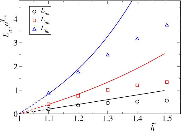
Figure 5: Onsager coefficients versus $\tilde{h}$. Symbols refer to numerical simulations while solid lines are the analytic estimates obtained from Eq. (30). Lower, middle and upper data refer respectively to $L_{aa}$, $L_{ah}$ and $L_{hh}.$ Dashed lines are obtained from the low-temperature expressions in Eq. (31). Simulations were obtained for $a=1$.

It is now interesting to discuss the origin of this discrepancy, because the passage from a full circle to three arcs has two effects on our MMC algorithm. When the three masses of a triplet $(c_{1},c_{2},c_{3})$ are sufficiently heterogeneous, the intersection between the plane of constant mass and the sphere of constant energy is the union of three disjoint arcs rather than a single connected circle [18]. For this class of moves, the analytic result of Eq. (30) overestimates the stationary flux, as it assumes that the rotation angle $\theta$ in Eq. (3.1) always varies in $[0,2\pi)$. In B we clarify that the main contribution to the observed deviations derives from the pinning property of localized states imposed by the C2C dynamics, i.e. the fact that a sufficiently large peak cannot jump to neighboring sites. When pinning is removed (see Ref. [28] for a discussion of this modification of the model), we find a better agreement with the analytic estimate, which extends to higher $\tilde{h}$ values.

3.2 High temperature limit

In this section we determine the Onsager coefficients for a point located in the critical curve at infinite temperature, $(m_{0},\beta_{0})=(-1,0)$, corresponding to $a_{0}=1$ and $\tilde{h}_{0}=2$. Such a critical point calls for caution because results obtained at finite $T$ might not be valid and Onsager coefficients might have some nonanalytic behavior.

For this reason we have performed a detailed numerical investigation in order to ensure significantly accurate simulations. More precisely, we have generated several parametric curves, all starting in $(m_{0},\beta_{0})$ and terminating in different points $(m_{i},\beta_{i})$. The resulting paths are plotted in Fig. 6. All simulations are done in a system of length $N=160$. A comparison with length $N=320$ (not shown) confirms that these results are asymptotic. In order to extract $\beta$ and $m$ from the numerical simulations, we have made use of Eqs. (6,7) with the help of the perturbative expansion in Eq. (10).

Fifteen curves are entirely located in the homogeneous $\beta\geq 0$ region and will be employed to determine the coefficients $L_{uv}(-1,0)$. Note that three curves (the two leftmost ones and the rightmost one) cross the critical line at infinite temperature thus entering the negative-temperature region of the model. We will further investigate this phenomenon in Sec. 5.

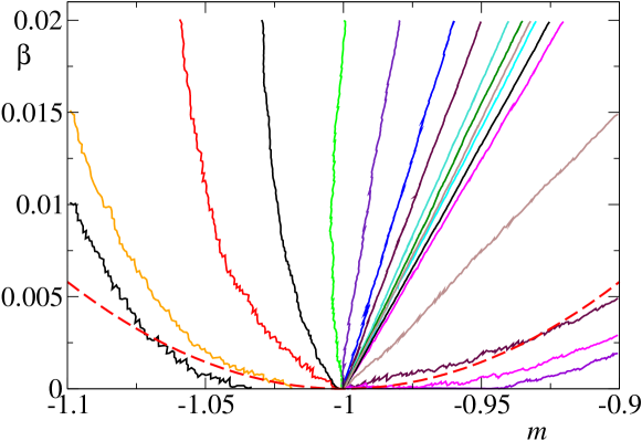
Figure 6: Different stationary paths in the $m$, $\beta$ plane. All curves terminate in the infinite-temperature point $(m_{0},\beta_{0})$. The red dashed line represents the analytic approximation of the path tangent to $\beta=0$ in $m=-1$, see Sec. 5.

We proceed by first averaging Eqs. (12-13) over all simulations, assuming that the coefficients $L_{u,v}(-1,0)$ do not depend on the slope of the path. The consistency of this assumption will be verified a-posteriori. We therefore write

$$\langle j_{a}\rangle = -L_{aa}\langle m_{y}\rangle+L_{ah}\langle\beta_{y}\rangle$$ (32)

$$\langle j_{h}\rangle = -L_{ha}\langle m_{y}\rangle+L_{hh}\langle\beta_{y}\rangle$$ (33)

obtaining

$$L_{ah} = \frac{\langle j_{a}\rangle}{\langle\beta_{y}\rangle}+\frac{\langle m_{y}\rangle}{\langle\beta_{y}\rangle}L_{aa}$$ (34)

$$L_{ha} = -\frac{\langle j_{h}\rangle}{\langle m_{y}\rangle}+\frac{\langle\beta_{y}\rangle}{\langle m_{y}\rangle}L_{hh}.$$ (35)

Then we replace these expressions in the original equations (12-13), now indexed by $i=1,\dots,15$ to clarify that each one refers to a different parameteric curve shown in Fig. 6,

$$-j_{a}^{i}\langle\beta_{y}\rangle+\langle j_{a}\rangle\beta_{y}^{i} = L_{aa}\left(m_{y}^{i}\langle\beta_{y}\rangle-\langle m_{y}\rangle\beta_{y}^{i}\right)$$ (36)

$$-j_{h}^{i}\langle m_{y}\rangle+\langle j_{h}\rangle m_{y}^{i} = L_{hh}\left(m_{y}^{i}\langle\beta_{y}\rangle-\langle m_{y}\rangle\beta_{y}^{i}\right).$$ (37)

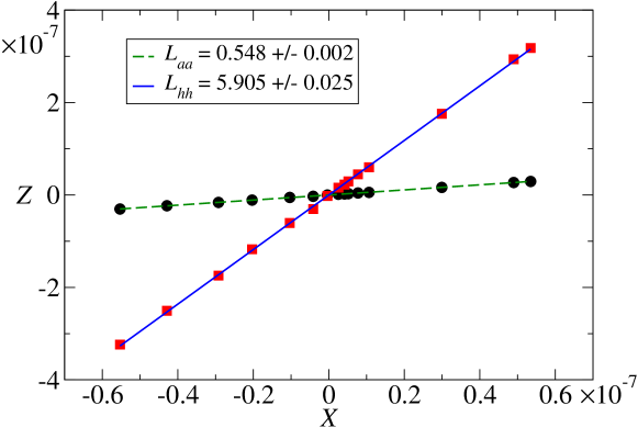
Figure 7: Inferring the diagonal elements of the Onsager matrix in the space $(X,Z)$, see Eqs. (36-37).

The two equations are of the type $Z^{i}=L_{uv}X^{i}$, where $X^{i}=m_{y}^{i}\langle\beta_{y}\rangle-\langle m_{y}\rangle\beta_{y}^{i}$. The resulting data are reported in Fig. 7 in the space $(X,Z)$. As expected, the data are well aligned along straight lines; their slopes yield the two diagonal coefficients of the Onsager matrix. By then using the formulas (34-35) for the off-diagonal elements, we find that $L_{ah}\sim 1.57\pm 0.03$ and $L_{ha}\sim 1.59\pm 0.03$, compatible with the theoretical expectation that they must coincide.

By now invoking the scaling form of the Onsager coefficients of Eq. (3), we can extend the above result to the whole infinite-temperature line. Since the variable $z=m/\sqrt{\beta}$ is constant along this line, and equal to minus infinity, we obtain

$$L_{uv}(m,\beta=0)=|m|^{\gamma_{uv}}L_{uv}(-1,0),$$ (38)

where the coefficients $L_{uv}(-1,0)$ have just been determined. We can therefore conclude that the Onsager matrix remains finite and well-defined on the $\beta=0$ line.

4 Spatial correlations

The analytic approach discussed in Sec. 3.1 clarifies that in the low-temperature regime correlations do not play any role for the determination of the Onsager coefficients. On the other hand, it is reasonable to expect that for sufficiently high temperatures transport coefficients do depend on nonequilibrium correlations. In this section we analyze the role of correlations and quantify their importance for the coupled transport problem. For this purpose we focus on a regime close to $\beta=0$ and consider the following setup. The reservoir on the right boundary imposes $\beta_{R}=0$ and $m_{R}=-1$, while the left reservoir imposes $m_{L}=m_{R}$ and $\beta_{L}=\Delta\beta$, with $\Delta\beta=0.1$ (this corresponds to a line approximately vertical in Fig. 6). To keep the amplitude of finite-size effects under control, two lattice lengths $N=50$ and $N=100$ are here compared.

We compute the covariance matrix

$$C_{ij}=\langle c_{i}c_{j}\rangle-\langle c_{i}\rangle\langle c_{j}\rangle$$ (39)

where $\langle\cdot\rangle$ refers, as before, to the average over the nonequilibrium stationary measure. The diagonal elements $C_{ii}=h_{i}-a_{i}^{2}$ correspond to the local variance of the mass along the chain and do not provide information on correlations.

Off-diagonal elements of $C_{ij}$ are expected to vanish as the gradient of $\beta$ goes to zero. For this reason, it is convenient to rescale the correlation matrix with the gradient of $\beta$,

$$\tilde{C}_{ij}=NC_{ij}/\Delta\beta.$$ (40)

In Fig. 8 we show the main features of $\tilde{C}_{ij}$, as found from numerical simulations. In panel (a) we report the nearest-neighbor correlations (located in the upper diagonal $\tilde{C}_{i,i+1}$) as a function of the rescaled position $y=i/N$. A nontrivial correlation pattern is obtained, characterized by an asymmetric distribution of positive and negative correlations. In panel (b) we show the behavior of $\tilde{C}_{k,i}$ while moving along the entire row corresponding to the central lattice site $k=N/2$. Similarly to other nonequilibrium models (see e.g. Ref. [30]), long-range correlations are found of amplitude $1/N$ across the entire system.

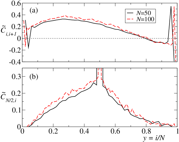
Figure 8: (a) Upper diagonal of the rescaled correlation matrix $\tilde{C}_{ij}$ for $N=50$ (solid line) and $N=100$ (dashed line). The dotted line highlights the zero baseline. (b) Rescaled correlation matrix $\tilde{C}_{N/2,i}$ for the same lattice sizes.

To better understand the role of correlations for the Onsager matrix, we have considered a modified MMC dynamics restricted to a triplet $(N=3)$ in which correlations are intentionally suppressed . This can be realized by imposing on each site of the triplet independent distributions of the local masses, where the distribution on site $i$ is defined by parameters $(\beta_{i},m_{i})$ chosen in order to produce given constant gradients. In Fig. 9 we compare the three Onsager coefficients for the full MMC model (symbols) with those corresponding to the uncorrelated model (solid lines). As expected, in the low-temperature region correlations are very small for the MMC dynamics and $L_{u,v}$ are well described by the fully uncorrelated model. On the other hand, for larger $\tilde{h}$ correlations tend to decrease the values of the Onsager coefficient with respect to the uncorrelated limit. This effect is maximal for the infinite-temperature point $\tilde{h}=2$ and clarifies that the peculiar structure of $L_{uv}$ found in this limit depends at least in part on nonequilibrium correlations.

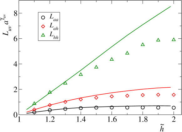
Figure 9: Onsager coefficients versus $\tilde{h}$. Symbols refer to numerical simulations of the MMC model (same data of Fig. 4), while solid lines are obtained for the fully uncorrelated dynamics, see text. Lower, middle and upper data series refer respectively to $L_{aa}$, $L_{ah}$ and $L_{hh}$.

5 Spontaneous emergence of negative temperatures

In Ref. [28], it was shown that nonequilibrium stationary paths can enter the negative-temperature region even when the reservoirs at the chain boundaries impose positive temperatures. As a result, a new kind of condensation phenomenon may arise, produced exclusively in nonequilibrium conditions. In this section, we revisit this process from the point of view of Onsager theory, deriving a perturbative expression of the limiting form of the paths and, accordingly, the condition for them to enter the negative$-T$ region.

We start the analysis by focusing on the shape of the paths that are nearly tangent to the $\beta=0$ line, see e.g. the second rightmost curve in Fig. 6. Each stationary path is by definition characterized by constant mass $(j_{a})$ and energy $(j_{h})$ currents. It is convenient to take their ratio $\rho$ because we can get rid of the explicit spatial dependence of $\beta$ and $m$. In fact, from Eqs. (12) and (13),

$$\rho=\frac{j_{a}}{j_{h}}=\frac{L_{aa}-L_{ah}\beta_{m}}{L_{ha}-L_{hh}\beta_{m}}=\frac{|m|\overline{L}_{aa}(z)-\beta_{m}\overline{L}_{ah}(z)}{|m|\overline{L}_{ha}(z)-\beta_{m}\overline{L}_{hh}(z)}|m|$$ (41)

where $\beta_{m}=d\beta/dm=\beta_{y}/m_{y}$.

A first relevant consequence of the above relation is that the isothermal line $\beta(m)=0$ cannot correspond to a stationary path. Indeed, along this line Eq. (41) would write

$$\rho=\frac{\overline{L}_{aa}(-\infty)}{\overline{L}_{ha}(-\infty)}|m|\;.$$ (42)

Since the ratio of Onsager coefficients is finite along the critical line $\beta=0$ (see Eq. (38)), the ratio $\rho$ would grow linearly with $|m|$, contradicting the physical condition of a constant $\rho$ along a NESS path.

We now relax the condition $\beta(m)=0$ and investigate the occurrence of tangent paths. More precisely we assume

$$\beta(m)=g(m-m_{0})^{2}\equiv g\delta^{2}\,;\quad m=m_{0}+\delta\,;\quad\delta\ll 1,$$ (43)

where $g$ is a coefficient determining the openness of the parabolic shape. In the vicinity of $m=m_{0}$, $|\beta_{m}|\ll 1$. Under this approximation, Eq. (41) can be written as

$$\rho=\frac{\overline{L}_{aa}(\sqrt{\beta}/m)}{\overline{L}_{ha}(\sqrt{\beta}/m)}|m|+\left(\frac{\overline{L}_{aa}(\sqrt{\beta}/m)\overline{L}_{hh}(\sqrt{\beta}/m)}{\overline{L}_{ah}^{2}(\sqrt{\beta}/m)}-1\right)\beta_{m},$$ (44)

where we have expressed the Onsager coefficients $\overline{L}_{uv}$ as functions of $w\equiv 1/z=\sqrt{\beta}/m$, rather than as functions of $z$, which diverges in the limit $\beta=0$.

By inserting the parabolic Ansatz for $\beta(m)$ into Eq. (44) and retaining all terms up to order $\delta$, we obtain

$$\rho=\frac{\overline{L}_{aa}(\sqrt{g}\delta/m_{0})}{\overline{L}_{ha}(\sqrt{g}\delta/m_{0})}(|m_{0}|-\delta)+2g\left(\frac{\overline{L}_{aa}(0)\overline{L}_{hh}(0)}{\overline{L}_{ah}^{2}(0)}-1\right)\delta,$$ (45)

where we have made explicit that the ratio of Onsager coefficients multiplying $(|m_{0}|-\delta)$ should be evaluated in $w=(\sqrt{g}/m_{0})\delta$. Eq. (45) can be further simplified by considering the linear expansion $\overline{L}_{uv}(w)=\overline{L}_{uv}(0)+\overline{L}^{\prime}_{uv}(0)w$. The derivative $\overline{L}^{\prime}_{uv}(0)$ is conveniently determined passing through the variable $\Delta=2-\tilde{h}$,

$$\left.\overline{L}^{\prime}_{uv}(w)\right|_{w=0} = \left.\overline{L}^{\prime}_{uv}(\Delta)\right|_{\Delta=0}\left.\frac{d\Delta}{dw}\right|_{w=0}$$ (46)

$$= \left.\overline{L}^{\prime}_{uv}(\Delta)\right|_{\Delta=0}2w|_{w=0}=0,$$ (47)

where the result follows from the combined numerical observation that: (i) all Onsager coefficients have a finite derivative with respect to $\tilde{h}$ (i.e., with respect to $\Delta$); (ii) $(d\Delta/dw)_{w=0}=2w|_{w=0}=0$.

As a result, the $\delta-$dependence of the Onsager coefficients can be neglected to this order and we obtain

$$\rho=\frac{\overline{L}_{aa}(0)}{\overline{L}_{ha}(0)}(|m_{0}|-\delta)+2g\left(\frac{\overline{L}_{aa}(0)\overline{L}_{hh}(0)}{\overline{L}_{ah}^{2}(0)}-1\right)\delta.$$ (48)

For this equation to be valid, it is necessary that $\rho$ is independent of $\delta$, therefore

$$\rho=\frac{\overline{L}_{aa}(0)}{\overline{L}_{ha}(0)}|m_{0}|$$ (49)

and

$$g=\frac{1}{2}\frac{\overline{L}_{ah}(0)\overline{L}_{aa}(0)}{\det\overline{L}(0)}\;.$$ (50)

The first condition determines the flux ratio along a path crossing tangentially the $\beta=0$ line in $m=m_{0}$. By inserting the value of the coefficients determined from the simulations, we obtain that $\rho\approx-0.348$ for $m_{0}=-1$. This value is consistent with the ratio observed in eventually tangent paths, see the second leftmost (orange) curve in Fig. 6, where $\rho\approx-0.344$. The second condition determines the concavity of the path. Interestingly, it is independent of $m_{0}$, meaning that the concavity is constant along the $\beta=0$ line. More precisely, we find that $g\approx 0.58$, in agreement with the concavity of the various paths, see the red dashed line in Fig. 6.

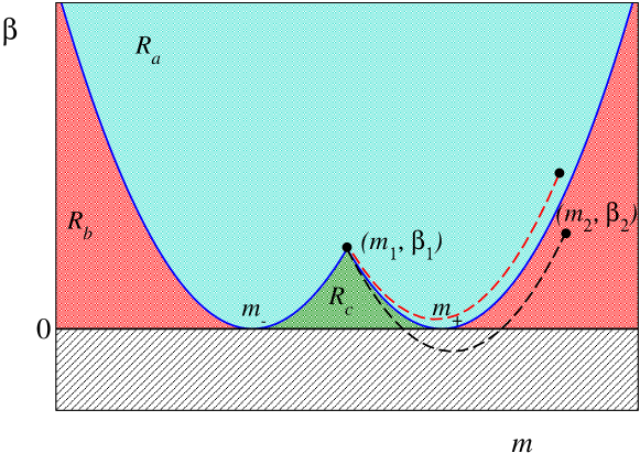
Figure 10: Stationary paths starting from $(m_{1},\beta_{1})$ can be of three types, depending on the region where they terminate. If the second reservoir $(m_{2},\beta_{2})$ is located in $R_{a}$ ($R_{c}$), all the path is contained in $R_{a}$ ($R_{c}$), and negative temperatures do not appear (red dashed line). If the second reservoir is located in $R_{b}$, the path is initially contained in $R_{c}$, then it attains the condensed phase (grey region), and finally it re-enters the positive$-T$ region in $R_{b}$ (black dashed line). $m_{\pm}$ are the values of $m$ where the limiting paths starting from $(m_{1},\beta_{1})$ are tangent to the critical line $\beta=0$.

We now focus our attention on the emergence of paths entering the $T<0$ condensed phase. Let us suppose that one end of the chain is thermalized at $(m_{1},\beta_{1})$ (see Fig. 10). Two NESS paths depart from this point, that are tangent to the infinite temperature line. If $\beta_{1}$ is small, we can rely on the parabolic approximation in Eq. (43) writing $\beta_{\pm}=g(m-m_{\pm})^{2}$, where $g$, given by Eq. (50), is the same in both curves. By imposing that the parabolas pass through $(m_{1},\beta_{1})$, it follows that $m_{\pm}=m_{1}\pm\sqrt{\beta_{1}/g}$. It is easily seen that these two curves partition the parameter space into three regions $R_{a}$, $R_{b}$, and $R_{c}$ (see Fig. 10). If and only if the other end of the system is located in the region $R_{b}$, the corresponding path enters the negative temperature region; otherwise, the entire path is characterized by positive temperatures. This property follows from the fact that the family of all stationary paths departing from $(m_{1},\beta_{1})$ cannot cross the two limiting parabolas. Indeed, upon calling $(m_{c},\beta_{c})$ the point of intersection, this would imply the existence of two distinct paths connecting $(m_{1},\beta_{1})$ with $(m_{c},\beta_{c})$. However, ergodicity implies the existence of a single path, the one minimizing dissipation [31].  Formally, if the two reservoirs are located in $(m_{1},\beta_{1})$ and $(m_{2},\beta_{2})$, with $m_{2}>m_{1}$, the path enters the condensed phase if

$$m_{2}>m_{1}+\sqrt{\frac{\beta_{1}}{g}}$$ (51)

and

$$\beta_{2}<g\left(m_{2}-m_{1}-\sqrt{\frac{\beta_{1}}{g}}\right)^{2}.$$ (52)

These conditions are exact in the limit of large temperatures, i.e. for vanishing $\beta_{1,2}$. In Fig. 10 we show qualitatively a path entering the condensed region (black dashed line) and a path fully confined in the positive-temperature region (red-dashed line). Similar considerations could be done in the microcanonical parameter space $(a,h)$, using Eqs. (6-7). Here we limit to report the expression of the steady path tangent to the critical curve $h=2a^{2}$ in the point $(a_{0},2a_{0}^{2})$:

$$h(a)=2a_{0}^{2}+4a_{0}(a-a_{0})+(2-4g)(a-a_{0})^{2}.$$ (53)

Since $g\simeq 0.58$, the coefficient of the quadratic term is negative and the curvature of the limiting path is therefore opposed to the positive curvature of the critical line.

Non-monotonic temperature profiles are typically observed in one-dimensional Hamiltonian models in the presence of thermomechanical forces [32, 33, 15]. Physically, it is a manifestation of the Joule effect, i.e. the heating of a wire induced by the flow of an irreversible current of mass (or charge). Here, the effect is extreme, as the inner temperatures become so large as to become negative. In more quantitative terms, the local heat production rate $\dot{Q}$ due to Joule heating can be expressed as (see Eq. (20) of Ref. [8])

$$\dot{Q}=\frac{j_{a}^{2}}{\beta L_{aa}}.$$ (54)

In the vicinity of the critical line, still neglecting the dependence of $L_{aa}$ on $\delta$, Eq. (54) rewrites as

$$\dot{Q}=\frac{j_{a}^{2}}{\overline{L}_{aa}(0)}\frac{m^{2}}{\beta}\,,$$ (55)

where $j_{a}$ and $m$ are finite, therefore clarifying that $\dot{Q}$ diverges with temperature. On the other hand, the corresponding contribution to entropy production rate, $\dot{Q}\beta$, remains finite.

For the sake of completeness it is worth mentioning that, as shown in Ref. [28], paths crossing the critical line, may no longer be characterized by a stationary dynamics. This phenomenon, however, does not affect the path shape in the positive-temperature region. Strictly stationary paths are, instead obtained, if the unrestricted variant of the model described in B is adopted [28].

6 Conversion efficiency

Coupled transport can be quantified in terms of the Seebeck coefficient defined as [8]

$$S\equiv\beta\frac{L_{ah}}{L_{aa}}-m\,.$$ (56)

By using the scaling relations for the Onsager coefficients, see Eq. (3), this expression can be rewritten in the form

$$S=m\left(\mbox{sign}(z)\frac{\overline{L}_{ah}(z)}{z^{2}\overline{L}_{aa}(z)}-1\right)\,,$$ (57)

therefore, in analogy with $L_{uv}$, it is sufficient to study $S/m$ as a function of $z$, or equivalently $Sa$ as a function of $\tilde{h}$.

In Fig. 11 we show the behavior of $Sa(\tilde{h})$ in the whole range $1\leq\tilde{h}\leq 2$ as obtained from numerical simulations (open symbols). We find that the Seebeck coefficient is positive and monotonically increasing with $\tilde{h}$.

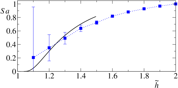
Figure 11: Scaled Seebeck coefficient $Sa$ versus $\tilde{h}$. Symbols refer to numerical simulations performed at $a=1$ while the solid line shows the low-energy analytic prediction obtained from Eq. (30). Vertical bars are an estimate of numerical errors, see the main text.

We also show as a solid line the analytic estimate obtained from Sec. 3.1 valid in the low-energy limit. From this result, we find that $Sa(\tilde{h})$ vanishes as $\tilde{h}\to 1$. The deviations observed in the numerical data in this regime are mostly due to numerical uncertainties in the determination of $L_{aa}$ and $L_{ah}$, which are amplified by the large value of $\beta$ in the definition (56), as highlighted by the increasing error bars with decreasing $\tilde{h}$. In the opposite limit $\tilde{h}\to 2$, $Sa(\tilde{h})$ converges to $1$, as immediately found from Eq. (56) for $\beta\to 0$ and $ma\to-1$, see Eq. (7).

In the presence of coupled transport, a measure of the efficiency of conversion of one current into another is provided by the dimensionless figure of merit

$$ZT=\frac{(L_{ah}-\frac{m}{\beta}L_{aa})^{2}}{\det{L}}$$ (58)

and by the related conversion efficiency

$$\frac{\eta}{\eta_{C}}=\frac{\sqrt{ZT+1}-1}{\sqrt{ZT+1}+1}\,,$$ (59)

where $\eta_{C}$ is the Carnot efficiency, see [8] for details. The ratio $\eta/\eta_{C}$ increases from $0$ for $ZT\ll 1$ to $1$ for $ZT\gg 1$.

The parameter $ZT$ is readily rewritten as a function of the sole variable $z$, namely

$$ZT=\frac{\left(\mbox{sign}(z)\overline{L}_{ah}(z)-z^{2}\overline{L}_{aa}(z)\right)^{2}}{\det\overline{L}(z)}.$$ (60)

The dependence of ZT and $\eta$ on $\tilde{h}$ are reported in Fig. 12 (see the open symbols in panels (a) and (b)); the solid lines correspond to the low-energy analytic estimates.

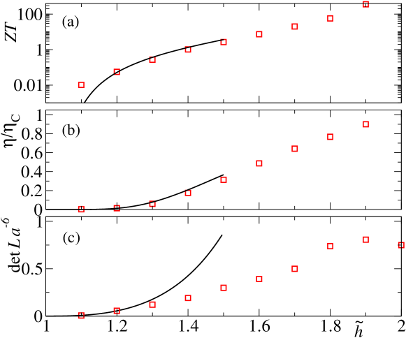
Figure 12: (a) Figure of merit $ZT$; (b) Conversion efficiency; (c) Determinant of the Onsager matrix versus $\tilde{h}$. Symbols refer to numerical simulations while solid curves illustrate the analytic prediction obtained from Eq. (30).

$ZT$ diverges in the infinite-temperature limit where, consequently, the efficiency reaches the Carnot limit. This behavior is not due to the vanishing of the determinant of $L$ in Eq. (58), as found for delta-energy filtering [34]. As it can be easily inferred from Eq. (58), the divergence of $ZT$ is related to: i) the finiteness of $L_{uv}$ and of its determinant (see Fig 12(c)) ii) the divergence of $\mu=m/\beta$.

We can argue that this behavior originates from the fact that infinite-temperature states are attained for a finite energy density $(\tilde{h}=2)$. Let us, in fact, consider the expression of the energy current, $j_{h}\simeq L_{hh}\nabla\beta\simeq-\nabla h$, where, for simplicity, we neglect the off-diagonal term due to the gradient of $m=\mu\beta$ and assume a direct proportionality with the energy density gradient $\nabla h$. From the boundedness of $h$ for vanishing $\beta$, $(2-h)\simeq\beta$ in the C2C model, one obtains $\nabla\beta\sim-\nabla h$. Accordingly, a finite current requires $L_{hh}$ to be finite. Conversely, for standard systems where the energy density diverges with temperature, e.g. $h\sim T^{\alpha}$ with $\alpha>0$, $\nabla\beta\sim\beta^{\alpha+1}\nabla h$ and a finite current implies a diverging $L_{hh}\sim 1/\beta^{\alpha+1}$.

7 Conclusions and perspectives

In this paper we conducted a fairly detailed study of the transport properties of a simple one-dimensional model with two conserved quantities: the mass density $a$ and the energy density $h$. This model is known to display an equilibrium localization transition when $h$ passes through the critical value $h_{c}=2a^{2}$ and an out-of-equilibrium localization transition if the system is boundary-driven by suitable reservoirs attached to its ends.

Because of a scaling relation, the dependence of all thermodynamic variables on $a$ and $h$ can be reduced to the dependence on a single quantity, typically identifiable with the relative energy density $h/a^{2}$. This includes the Onsager coefficients that we have thoroughly explored in the homogeneous region, $h\leq h_{c}$.

One of the main outcomes of our study is that a linear-response description of irreversible transport processes may apply even for arbitrarily large temperatures. Indeed we prove that Onsager coefficients have a smooth behavior up to the critical curve $T=\infty$, along which they exhibit a simple power-law dependence on $m=\mu\beta$. Moreover, we have shown that their behavior along the critical line is such that there exists a class of NESS paths in the $(m,\beta)$ plane that must enter the condensed region. Negative temperatures are therefore naturally attained by an out-of-equilibrium setup employing reservoirs at positive temperature. This mechanism suggests a novel effective protocol for the generation of negative-temperature states, which deserve further studies. In fact, one of the main experimental difficulties in this field concerns the ability to thermalize a system at negative temperature (see [26] for a review on the topic and [35] for a recent experiment).

We have also provided a direct evidence that the Onsager coefficients do depend on nonequilibrium correlations and we have identified the largest contribution in correspondence of the critical line of the model. Some peculiarities occurring for $T\to\infty$, like the divergence of the figure of merit $ZT$, are due to the finiteness of Onsager coefficients in such limit, a property that is strictly related to the finiteness of the energy density when $T$ diverges.

Last but not least, in the low-temperature limit we have obtained an analytic description of the nonequilibrium thermodynamic observables which compares successfully with the numerical results, especially if the dynamical rule allows peaks to diffuse. To our knowledge, this is one of the few examples in which the whole Onsager matrix is exactly computable for an interacting model. We have shown that in this limit, spatial correlations are absent. Nevertheless, coupled transport is still present, with a positive Seebeck coefficient.

Concerning the perspectives of our work, we expect that several features observed in the nonequilibrium C2C model are relevant also for the DNLS equation and its applications. Two important distinctions, however, should be emphasized. First of all no exact scaling properties hold in the DNLS equation because its total energy is made of two terms which scale differently with the mass [36]. The presence of an interaction (hopping) term is particularly relevant at low-temperatures, where we expect substantial differences between the two models. As an example, the Seebeck coefficient was found to change sign in the homogeneous region of the DNLS equation [33, 15], while in the C2C model it is always positive, see Fig. 11. Secondly, the Hamiltonian character of the DNLS dynamics is certainly richer than the stochastic MMC dynamics employed for the C2C model. In particular, we expect that dynamical effects will be relevant in the localized region of the DNLS model, where the existence of an adiabatic invariant freezes the macroscopic dynamics when high peaks appear in the system [37]. Because of that, the investigation of NESS profiles and Onsager coefficients in such a region is computationally very demanding. There are, however, reasons to think that it would be worth investigating their behavior.

More specifically, it is reasonable to expect that, similarly to the C2C model, DNLS profiles can cross the critical line when driven by reservoirs in the homogeneous region. In fact, in Ref. [29] some of us studied the DNLS equation in a nonequilibrium setup analogous to that used later in Ref. [28]: the DNLS chain was attached to a standard reservoir on one boundary and to a dissipator on the other boundary. The dissipator, called sink in the title, steadily removes mass and energy from the lattice and it can be thought of as a boundary condition imposing $a=h=0$. Within such set-up the system enters the localized region accompanied by a complicated dynamics.

Appendix A Perturbative analysis

In this appendix, we derive the limiting expressions (10), using Eqs. (6-7) or, more precisely,

$$\tilde{m}(z) = \frac{z^{2}}{2}+\frac{z}{\sqrt{\pi}}\frac{\mathrm{e}^{-z^{2}/4}}{1+\mathrm{erf}(z/2)},$$ (61)

$$\tilde{h}(z) = \frac{z^{2}}{2}\left(\frac{1}{\tilde{m}^{2}(z)}+\frac{1}{\tilde{m}(z)}\right).$$ (62)

In the limit $T\to 0$, $\tilde{h}\to 1$ and $z\to+\infty$, therefore $\tilde{m}(z)\simeq z^{2}/2$ and $\tilde{h}(z)\simeq 1+2/z^{2}$, i.e.

$$z=\sqrt{\frac{2}{\tilde{h}-1}},\;\;\mbox{for}\;\tilde{h}\to 1.$$ (63)

In the limit $T\to\infty$, $\tilde{h}\to 2$, $z\to-\infty$ and calculations are more lengthy. By accurately expanding the error function,

$$\mathrm{erf}(z/2)=-1+\frac{2\mathrm{e}^{-|z|^{2}/4}}{|z|\sqrt{\pi}}\left[1-\frac{2}{|z|^{2}}+\frac{12}{|z|^{4}}-\frac{120}{|z|^{6}}\right]\;,$$ (64)

we find that $\tilde{m}(z)\simeq-1+(4/z^{2})-(40/z^{4})$ and $\tilde{h}(z)\simeq 2-4/z^{2}$, i.e.

$$z=-\frac{2}{\sqrt{2-\tilde{h}}},\;\;\mbox{for}\;\tilde{h}\to 2.$$ (65)

Appendix B Evolution without pinning

As explained in the main text and sketched in Fig. 3, the new state in each MMC move must be chosen within the intersection between a sphere and a plane with the constraint of positive masses; this means either within a full circle or within three disconnected arcs. In the latter case, there are two selection options: within the same arc as in the original configuration; within any of the three arcs with equal probability.

Since the three-arcs solution appears when one mass is significantly larger than the other two, these two options correspond to either pin a peak, or to allow it diffusing. All of our simulations in the main text have been made following the former option. This choice originates from the DNLS equation, where peaks are dynamically pinned [37]. Here below we consider the second option as it helps singling out the role of diffusion at higher temperatures.

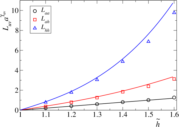
Figure 13: Onsager coefficients versus $\tilde{h}$ for the unpinned MMC dynamics. Continuous lines are analytic estimates obtained from Eq. (30), symbols refer to numerical simulations. Lower, middle and upper data refer respectively to $L_{aa}$, $L_{ah}$ and $L_{hh}$.

In fact, when $T$ increases and the three-arcs solution is increasingly likely, the low-$T$ approximation fails in two respects: i) it averages over angles corresponding to unphysical negative masses; ii) it allows diffusion to the neighboring arcs. If we adopt a no-pinning evolution, only i) applies. In Fig. 13 we compare the low-$T$ approximation with the numerical outcome of the unpinned model. The agreement extends to significantly larger energy densities; in fact, allowing peaks to diffuse, the Onsager (transport) coefficients are now significantly larger.

References

References

- [1] Sornette D 2006 Critical phenomena in natural sciences: chaos, fractals, selforganization and disorder: concepts and tools (Springer Science & Business Media)
- [2] Touchette H 2009 Physics Reports 478 1–69
- [3] Lepri S, Livi R and Politi A 2003 Physics reports 377 1–80
- [4] Lepri S 2016 Thermal transport in low dimensions: from statistical physics to nanoscale heat transfer vol 921 (Springer, Heidelberg)
- [5] Livi R 2022 Physica A: Statistical Mechanics and its Applications 127779
- [6] Spohn H 2023 Hydrodynamic scales of integrable many-particle systems URL https://arxiv.org/abs/2301.08504
- [7] Lepri S, Livi R and Politi A 2020 Physical Review Letters 125 040604
- [8] Benenti G, Casati G, Saito K and Whitney R S 2017 Physics Reports 694 1–124
- [9] Benenti G, Casati G and Mejía-Monasterio C 2014 New Journal of Physics 16 015014
- [10] Livi R and Politi P 2017 Nonequilibrium statistical physics: a modern perspective (Cambridge University Press)
- [11] Klumpp S 2003 Journal of Statistical Physics 113 233
- [12] Kipnis C, Marchioro C and Presutti E 1982 Journal of Statistical Physics 27 65–74
- [13] Basile G, Bernardin C and Olla S 2006 Physical review letters 96 204303
- [14] Maes C and Van Wieren M H 2005 Journal of Physics A: Mathematical and General 38 1005
- [15] Iubini S, Lepri S, Livi R and Politi A 2016 New Journal of Physics 18 083023
- [16] Kevrekidis P G 2009 The discrete nonlinear Schrödinger equation: mathematical analysis, numerical computations and physical perspectives vol 232 (Springer Science & Business Media)
- [17] Iubini S, Franzosi R, Livi R, Oppo G L and Politi A 2013 New Journal of Physics 15 023032
- [18] Iubini S, Politi A and Politi P 2014 Journal of Statistical Physics 154 1057–1073
- [19] Iubini S, Politi A and Politi P 2017 Journal of Statistical Mechanics: Theory and Experiment 2017 073201
- [20] Barré J and Mangeolle L 2018 Journal of Statistical Mechanics: Theory and Experiment 2018 043211
- [21] Arezzo C, Balducci F, Piergallini R, Scardicchio A and Vanoni C 2022 Journal of Statistical Physics 186 1–23
- [22] Szavits-Nossan J, Evans M R and Majumdar S N 2014 Physical review letters 112 020602
- [23] Szavits-Nossan J, Evans M R and Majumdar S N 2014 Journal of Physics A: Mathematical and Theoretical 47 455004
- [24] Gotti G, Iubini S and Politi P 2021 Physical Review E 103 052133
- [25] Gradenigo G, Iubini S, Livi R and Majumdar S N 2021 Journal of Statistical Mechanics: Theory and Experiment 2021 023201 URL https://doi.org/10.1088/1742-5468/abda26
- [26] Baldovin M, Iubini S, Livi R and Vulpiani A 2021 Physics Reports 923 1–50
- [27] Gradenigo G, Iubini S, Livi R and Majumdar S N 2021 The European Physical Journal E 44 1–6
- [28] Gotti G, Iubini S and Politi P 2022 Physical Review E 106 054158
- [29] Iubini S, Lepri S, Livi R, Oppo G L and Politi A 2017 Entropy 19 445
- [30] Bertini L, De Sole A, Gabrielli D, Jona-Lasinio G and Landim C 2009 Journal of Statistical Physics 135 857 URL https://doi.org/10.1007/s10955-008-9670-4
- [31] Onsager L 1945 Ann N Y Acad Sci. 46 241–265
- [32] Iacobucci A, Legoll F, Olla S and Stoltz G 2011 Physical Review E 84 061108
- [33] Iubini S, Lepri S and Politi A 2012 Physical Review E 86 011108
- [34] Mahan G and Sofo J 1996 Proceedings of the National Academy of Sciences 93 7436–7439
- [35] Baudin K, Garnier J, Fusaro A, Berti N, Michel C, Krupa K, Millot G and Picozzi A 2023 Phys. Rev. Lett. 130(6) 063801
- [36] Rasmussen K, Cretegny T, Kevrekidis P G and Grønbech-Jensen N 2000 Physical review letters 84 3740
- [37] Iubini S, Chirondojan L, Oppo G L, Politi A and Politi P 2019 Physical review letters 122 084102