Abstract

In this work, we have developed an FLRW type model of a universe which displays transition from deceleration in the past to the acceleration at the present. For this, we have considered field equations of f(R,T) gravity and have taken $f(R,T)=R+2\lambda T$, $\lambda$ being an arbitrary constant. We have estimated the $\lambda$ parameter in such a way that the transition red shift is found similar in the deceleration parameter, pressure and the equation of state parameter $\omega$. The present value of Hubble parameter is estimated on the basis of the three types of observational data set: latest compilation of $46$ Hubble data set, SNe Ia $580$ data sets of distance modulus and $66$ Pantheon data set of apparent magnitude which comprised of 40 SN Ia bined and 26 high redshift data’s in the range $0.014\leq z\leq 2.26$. These data are compared with theoretical results through the $\chi^{2}$ statistical test. Interestingly, the model satisfies all the three weak, strong and dominant energy conditions. The model fits well with observational findings. We have discussed some of the physical aspects of the model, in particular the age of the universe.

Keywords: $f(R,T)$ theory; FLRW metric; Observational parameters; Transit universe; Observational constraints
PACS number: 98.80-k, 98.80.Jk, 04.50.Kd

1 Introduction

Cosmology as of now has become a very exciting and developing domain of knowledge in which we study how the universe originates(Hot Big bang)and evolve over the time(Inflation, Era of subatomic heavy and light particles, radiation and present day matter dominated Era) [1] $-$ [3]. Latest surveys and observations [4] $-$ [26] predict the presence of ‘Exotic and dynamic dark energy(DE) and opposite to it stationary cold dark matter(CDM) both in abundance. While CDM deviates the path of light and produces gravitational lensing, DE creates negative pressure and separates baryon galaxies and clusters from each other and creates acceleration in them. These two provide a larger observed value of critical density and distance modulus of luminous objects.

Before these developments, the universe was best modeled by a well known standard FLRW spacetime which is spatially homogeneous and isotropic (Refer [3] for details). The model originates with an unavoidable singularity representing bigbang. If the content of the universe can be assumed as a perfect fluid then it represents a decelerating expanding universe. This means that galaxies as fluid particles are moving away from one another with a relatively dampening pace over time.

In order to attribute acceleration in the FLRW model, cosmological constant $\Lambda$ was resurrected and introduced in the Einstein field equation. It opined that $\Lambda$ supports the acceleration $\ddot{a}/a$ and opposes barion pressure so it is anti gravity and produces negative pressure. New cosmology is given the name $\Lambda$ CDM ([27] $-$ [29]). Under this, it is proposed that nearly 27% of the total content of the universe is CDM and $\eqsim 70\%$ is dark energy which is interpreted as $\Lambda$ energy. $\Lambda$ CDM is also called a concordance model, which is accepted by all the scientific community. But this model lacks in explaining fine tuning and cosmic coincidence problems[30]. To avoid this, quintessence and phantom models [31] $-$[35] were developed in which scalar field $\phi$ represents dark energy and satisfies the following equation of motion $\ddot{\phi}+3H\dot{\phi}+V^{\prime}=0.$ It is very interesting that this equation is equivalent to energy conservation equation $\dot{\rho}+3H(p+\rho)=0$ for perfect fluid filled universe, where $\rho=\frac{1}{2}\dot{\phi}^{2}+V(\phi)$ and $p=\frac{1}{2}\dot{\phi}^{2}-V(\phi).$ Later on so many parametrizations were proposed for scalar $\phi$ and some interesting cosmological models surfaced [36] $-$ [42].

Parallelly, a group of scientists thought of a need to modify Einstein Field equations in order to explain the present day acceleration in the universe. For this, in the Einstein-Hilbert action $S=\int(\frac{1}{16\pi G}(R+L_{m})\sqrt{-g}dx^{4},$ they replaced $R$ by arbitrary functions of R, Trace of Einstein $G_{ij}$ and Energy momentum tensor $T_{ij}$. Accordingly so many modified theories of gravity $f(R)$, $f(R,G)$, $f(R,T)$, $f(R,T^{\phi})$, $f(Q)$, $f(T,B)$ and many more were proposed ([43]$-$ [76]). The idea behind this is as follows. Einstein’s basic philosophy lies in the fact that matter and energy are equivalent and their presence in the universe being permanent in nature creates curvature in the spacetime representing it. In the Einstein field equations, the Ricci scalar $R$ represent curvature. In FLRW spacetime scale factor and its derivatives are related functionally with $R$. So by replacing it with some arbitrary non-linear function of R and T, we must see the change in the mechanical equations of General Relativity and we might get the universe accelerating instead of deceleration.

In this work, we tried to obtain an universe model based on the cosmological principle that the physical universe is spatially homogeneous and isotropic and that it displays transition from deceleration in the past to the acceleration at the present. For this, we solve $f(R,T)$ gravity field equations in the background of FLRW space time which represent a spatially homogeneous and isotropic universe. In order to get the desired result we have considered the simplest form of $f(R,T)$ as $f(R,T)=R+2\lambda T$, where $\lambda$ is an arbitrary constant. While working with a universe model, one has to take care of the latest observational findings [20] $-$ [23]. In this contest estimations of present values of cosmological parameters like Hubble $H_{0}$, deceleration parameter $q_{0}$, growth of density, transition behaviour of pressure and equation of state parameter become crucial. Seeing the complex structure of the universe which contains so many exotic energies like dark energy in abundance, dark matter, black holes etc, roll of higher order derivative para meters like jerk, snap and lurk parameters become also crucial. Our universe at large scale is very much discipline. This is the reason that a very simple $\Lambda$CDM concordance model fits well on observational ground. In this model jerk parameter $j=1$. In this paper too, we have been successful to develop a universe model in $f(R,T)$ gravity with constant jerk parameter. The interesting part in the paper is that $\lambda$ parameter is chosen in such a way that the transition red shift is found similar in deceleration parameter, pressure and the equation of state parameter $\omega$ and that the model satisfies all the three weak, strong and Dominant energy conditions. The present value of Hubble parameter is estimated on the basis of the three types of observational data set: latest compilation of $46$ Hubble data set, SNe Ia $580$ data sets of distance modulus and 66 Pantheon data set of apparent magnitude which comprised of 40 SN Ia binned and 26 high redshift data’s in the range $0.014\leq z\leq 2.26$. These data are compared with theoretical results through the $\chi^{2}$ statistical test. The model fits well with observational findings. We have discussed some of the physical aspects of the model in particular age of the universe.

The paper is presented in the following section wise form. In section $2$, the $f(R,T)$ field equations have been presented and are solved for spatially homogeneous and isotropic FLRW space time by taking the content in the universe as perfect fluid and accordingly we have taken energy momentum tensor as that of perfect fluid. We arrive at the two equations in which first one may be called equation of motion of a fluid particle as it contains second order derivative of scale factor in form of deceleration constant and the pressure term in the right hand side of the equation. The other second equation provides rate of expansion as it contains Hubble parameter and density term in the right hand side of the equation. In this section we have solved density, pressure and equation of state parameter $\omega$ in term of Hubble and decelerating parameter so that they can be obtained once we know about the Hubble and decelerating parameter. In section $3$, deceleration and Hubble parameter were obtained by taking jerk parameter constant. It is interesting that decelerating parameter shows transition from negative to positive over red shift which means that in the past universe was decelerating and at present it is accelerating. In section $4$, density, pressure and the equation of state parameter $\omega$ were solved. The latter to show transition from present to past. We have estimated $\lambda$ parameter in such a way that the transition red shift is found similar in deceleration parameter, pressure and the equation of state parameter $\omega$. Energy conditions are evaluated and discussed in section $5$. Interestingly, the model satisfies all the three weak, strong and Dominant energy conditions. In section $6$, we have formulated distance modulus and apparent magnitude for our model and estimation of present value of Hubble parameter is done. As stated earlier, we have used the three types of observational data set: latest compilation of $46$ Hubble data set, SNe Ia $580$ data sets of distance modulus and $66$ Pantheon data set of apparent magnitude which comprised of $40$ SN Ia binned and $26$ high redshift data’s in the range $0.014\leq z\leq 2.26$. Figures and a table are properly presented to describe and analyse the results more clearly……………. In the last Section $8$, conclusions are provided.

2 f(R,T) gravity field equations for FLRW flat spacetime:

As it is said in the introduction that in the $f(R,T)$ gravity [56], the Ricci scar $R$ is replaced by an arbitrary function f(R,T) of $R$ and $T$, so we write the two actions and field equations as follows:

Einstein-Hilbert action:

$${}S=\int(\frac{1}{16\pi G}(R+2\lambda)+L_{m})\sqrt{-g}dx^{4}.$$ (1)

Einstein GR field equations:

$$R_{ij}-\frac{1}{2}Rg_{ij}+\Lambda g_{ij}=\frac{8\pi G}{c^{4}}T_{ij}.$$ (2)

f(R,T) gravity action:

$${}S=\int\Big{(}\frac{1}{16\pi G}f(R,T)+L_{m}\Big{)}\sqrt{-g}dx^{4},$$ (3)

and f(R,T) gravity field equations:

$${}R_{ij}-\frac{1}{2}Rg_{ij}=\frac{8\pi GT_{ij}}{f^{R}(R,T)}+\frac{1}{f^{R}(R,T)}\bigg{(}\frac{1}{2}g_{ij}(f(R,T)-Rf^{R}(R,T))-(g_{ij}\Box-\nabla_{i}\nabla_{j})f^{R}(R,T)+f^{T}(R,T)(T_{ij}+pg_{ij})\bigg{)},$$ (4)

where the energy momentum tensor $T_{ij}$ is related to the matter Lagrangian $L_{m}$ via the following equation

$${}T_{ij}=-\frac{2}{\sqrt{-g}}\frac{\delta(\sqrt{-g}L_{m})}{\delta g^{ij}}.$$ (5)

and $f^{R}$ and $f^{T}$ are the derivative of $f(R,T)$ with respect to $R$ and $T$ respectively. Three particular functional forms for arbitrary function $f(R,T)$ have been proposed for cosmology [56]. They are (a:) $R+2f(T)$ (b:) $f_{1}(R)+f_{2}(T)$ and (c:) $f_{1}(R)+f_{2}(R)f_{3}(T).$

We solve $f(R,T)$ gravity field equations (4 ) for FLRW spatially flat spacetime given by

$${}ds^{2}=dt^{2}-a^{2}(t)(dx^{2}+dy^{2}+dz^{2}),$$ (6)

by taking $L_{m}=-p$ and $f(R,T)=R+2\lambda T$ so that we get $T_{ij}$ as

$$T_{ij}=(\rho+p)u_{i}u_{j}-pg_{ij}.$$ (7)

and

$${}2\dot{H}+3H^{2}=-(8\pi+3\lambda)p+\lambda\rho$$ (8)

and

$${}3H^{2}=(8\pi+3\lambda)\rho-\lambda p,$$ (9)

where $H=\frac{\dot{a}}{a}$ is the Hubble parameter, $u^{i}u_{i}=1$ and $u^{i}u_{i;j}=0$. We assume $\lambda=8\pi\mu$. Then the field equations (8) and (9) are simplified as:

$${}(1-2q)H^{2}=8\pi(\mu\rho-(1+3\mu)p)$$ (10)

and

$${}3H^{2}=8\pi((1+3\mu)\rho-\mu p),$$ (11)

where $q=-\frac{\ddot{a}}{aH^{2}}$ is deceleration parameter and $\dot{H}=-(q+1)H^{2}$. Eqs. (10) and (11) are the two fundamental equations which describe equation of motion of a fluid particle which is commonly a galaxy and they do describe rate of expansion of the universe(Hubble parameter). As is mentioned in the introduction, our universe is accelerating so the two equations must explain it. For this both deceleration constant and the pressure must be negative. The observations tell us that luminous content of the universe (baryon fluid) is at present dust so the baryon pressure must be zero. But the literature [30] says that apart from baryon matter other energies do exist in the universe. It is estimated that nearly 28 % of the total content of the universe is dark matter which is responsible for the phenomenon of gravitating lensing occurring in the universe and nearly 68% of energy exists in the form of dark energy which is responsible for the present day acceleration in the universe. These ideas and how to accommodate them in the theories, have been explained in the introduction. In $f(R,T)$ gravity theory, Ricci scalar $R$ is replaced by an arbitrary function of $R$ and trace of energy momentum tensor $T$. The idea is that we must expect acceleration due to curvature and trace dominance. The authors feel that the pressure term arising in the field equations is not due to the baryonic content of the universe. It is as a result of the over all effect. We mean that terms containing $\mu$ in the field equations (10) and (11) are the extra terms in the original FLRW field equations of general relativity and they will have impact in producing pressure and creates acceleration in the universe. From Eqs. (10) and (11), we get, $\rho$, p and equation of state parameter $\omega=\frac{p}{\rho}$ as follows:

$$8\pi\rho=\frac{H^{2}(2\mu(q+4)+3)}{(2\mu+1)(4\mu+1)}$$ (12)

$$8\pi p=\frac{H^{2}((6\mu+2)q-1)}{(2\mu+1)(4\mu+1)}$$ (13)

and

$$\omega=\frac{p}{\rho}=\frac{(6\mu+2)q-1}{2\mu(q+4)+3}$$ (14)

3 Model with Constant Jerk and Transition Deceleration Parameters and their Evaluation from OHD Data Set:

There are two more parameters jerk and snap which are related with third and forth order of derivatives of scale factor. They play very important role in examining instability of a cosmological model. jerk is also one of the parameter in statefinder diagnostic. they are defined as: jerk $j=\frac{\dddot{a}}{aH^{3}}$ and snap $s=-\frac{\ddddot{a}}{aH^{4}}.$ The jerk parameter in the terms of deceleration parameter can be written as:

$${}j(z)=q(z)+2{q(z)}^{2}+(1+z)\frac{dq(z)}{dz}.$$ (15)

As jerk parameter ’$j$’ varies very slowly and its present value lies around 1 ( j = $1$ as per $\Lambda$CDM model), so we solve Eq.(15) for constant jerk i.e. we take j = constant. We obtain following expression for deceleration parameter.

$$q=\frac{1}{4}\left(-1+\sqrt{-8j-1}\text{Tan}\left[\frac{1}{2}\left(-2\tan^{-1}\left(\frac{4\sqrt{-8j-1}q_{0}+\sqrt{-8j-1}}{8j+1}\right)-\sqrt{-8j-1}\log(z+1)\right).\right]\right),$$ (16)

where we have used $q=q_{0}~{}\text{at~{} present}~{}i.e.~{}z=0.$ The deceleration parameter $q$ is related to Hubble parameter through the following differential equation.

$$H_{z}(1+z)=(q+1)H$$ (17)

so, using Eq. (16) and integrating Eq. (17), we may get the expression for Hubble parameters,

$$H=H_{0}e^{\int_{0}^{z}\frac{(q+1)dz}{(1+z)}}.$$ (18)

We note that the Eq. (18) has three unknown parameters $H_{0},~{}j~{}\text{and}~{}q_{0}.$

Now, we will estimate present value of Hubble parameter $H_{0}$. This will be done statistically. For this we consider a data set of $77$ observed values of Hubble constant at different red shift using (a). Cosmic chronometric method, (b). BAO signal in galaxy distribution and (c). BAO signal in Ly$\alpha$ forest distribution alone or cross-correlated with QSOs [77]$-$[91]. This data set is commonly known as OHD data set. We compare the data set values from those obtained theoretically from Eq. (18) by forming the following chi squire function of the present value of $H_{0},~{}j~{}\text{and}~{}q_{0}.$

$$\chi^{2}(H_{0},j,q_{0})=\frac{1}{46}\sum\limits_{i=1}^{46}\frac{[Hth(z_{i},H_{0},j,q_{0})-H_{ob}(z_{i})]^{2}}{\sigma{(z_{i})}^{2}},$$ (19)

Now the parameters $H_{0},~{}j~{}\text{and}~{}q_{0}.$ are estimated by getting the minimum value of chi squire for the values of $H_{0},~{}j~{}\text{and}~{}q_{0}.$ taken in the range (65$-$75), (0.95$-$1.05) and(-0.60 $-$ -0.45) respectively. It is found that $H_{0}=68.95,~{}j=0.95~{}\text{and}~{}q_{0}=-0.57$ , for minimum chi squire $\chi 2$ =0.5378. It may be be called a good fit. The fit will be more clear from the error bar and livelihood plots in the figure $1$. Before that, we rewrite Eq. (16) and integrate Eq. (18) by taking $q_{0}=-0.57$ and $j=0.95$ which are estimated values as per OHD data set. We get the following expressions for deceleration and Hubble parameters as:

$$q=\frac{0.483144\left((z+1)^{2.93258}-5.18713\right)}{(z+1)^{2.93258}+2.5491}$$ (20)

and

$$H=0.54H_{0}(1+z)^{0.017}(3.55+z(3+z(3+z)))^{0.489}$$ (21)

Figures $1(a)$ and $1(b)$ describe the growth of Hubble parameter $H$ and expansion rate $H/(1+z)=\dot{a}/a_{0}$ over red shift $`z^{\prime}$ respectively. Hubble parameter is increasing function of red shift which means that in the past Hubble constant was more. It is gradually decreasing over time. Expansion is high at present which indicates that universe is accelerating. These figures also show that theoretical graph passes near by through the dots which are observed values at different red shifts. Vertical lines are error bars. Figure $5(c)$ is likelihood probability curve for Hubble parameter. Estimated value $H_{0}=68.95$ is at the peak.

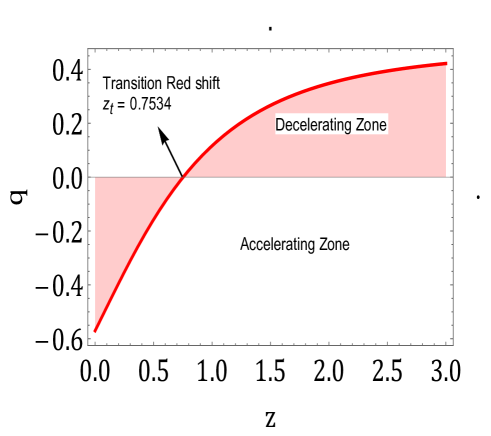
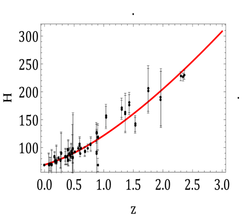
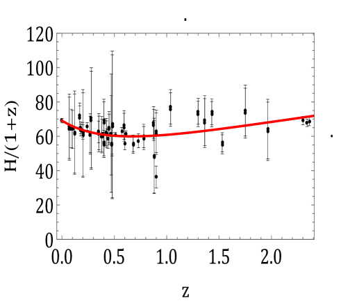
(a) (b) (c) (d)

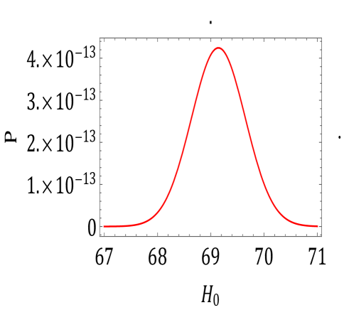
Figure 1: Figure (a) shows the growth of deceleration parameter $`q^{\prime}$ over red shift $`z^{\prime}$. It describes that in the past the universe was decelerating. At transition redshift $z_{t}$=0.7534, where $q\sim 0$, it changed its behaviour and started accelerating. Here $q_{0}=-0.57~{}\text{and}~{}j=0.95.$ Figures (b) and (c) are the error bar plots for Hubble parameter $H$ and expansion rate $H/(1+z)=\dot{a}/a_{0}$ over red shift $`z^{\prime}$ respectively. Figure (d) is likelihood probability curve for Hubble parameter. Estimated value $H_{0}=68.95$ is at the peak.

4 Expressions for Density, Pressure and Equation of State parameter of the Universe:

Having obtained expressions for deceleration, Hubble parameters and the value of $\mu$, we can obtain expressions for density $\rho$, pressure $p$ and equation of state parameter $\omega$from Eqs. (12)-(14) which are given as below:

$$\rho=\rho_{0}\frac{0.2916(z+1)^{0.034}(z(z(z+3)+3)+3.55)^{0.978}\left(2\mu\left(\frac{0.483144\left((z+1)^{2.93258}-5.18713\right)}{(z+1)^{2.93258}+2.54909}+4\right)+3\right)}{6.86\mu+3},$$ (22)

$$p=\text{p0}\frac{0.2916(z+1)^{0.034}(z(z(z+3)+3)+3.55)^{0.978}\left(\frac{0.483144(6\mu+2)\left((z+1)^{2.93258}-5.18713\right)}{(z+1)^{2.93258}+2.54909}-1\right)}{(6\mu+2)\text{q0}-1}$$ (23)

and

$$\omega=\frac{\mu\left(0.323307(z+1)^{2.93258}-1.67704\right)-0.00375986(z+1)^{2.93258}-0.843309}{1.71537\mu+1.\mu(z+1)^{2.93258}+0.334587(z+1)^{2.93258}+0.852892}$$ (24)

From Eq. (24), $\omega_{0}$ can be obtained from the parameter $\mu$ and $q_{0}$ as follows.

$$\omega_{0}=-\frac{0.094}{\mu+0.44}-0.499,$$ (25)

We see here that as universe is accelerating at present, so the pressure should be negative and as such the equation of state parameter $\omega_{0}$($p=\omega\rho)$ should also be negative, As per $\Lambda$ CDM and quintessence dark energy models $\omega_{0}=-1$ and $\omega_{0}\leq-1$. Like deceleration parameter $`q^{\prime}$, Eq. (24) also describe transition of equation of state parameter $\omega$ from negative values to positive values over red shift $`z^{\prime}$. This will make pressure of the universe also transitional which means that in the past pressure was positive and at present it is negative which creates acceleration in the universe. It is very interesting to see that $\omega=-0.0008$ at $z=0.7534$ for the value of parameter $\mu$ = 130. We note transition red shift for deceleration parameter $`q^{\prime}$ is also $z_{t}$=0.7534. So the traditional red shift for both deceleration parameter and equation of state parameter matches for $\mu$ = 130. This is very well seen in the following figure $2$ for $\omega$ and pressure. For drawing plot of pressure, we have replaced $p_{0}$ by $\omega_{0}\rho_{0}$. The value of $\omega_{0}$ is obtained from Eq. (25) as $\omega_{0}$=-0.499264 by taking $\mu$ = 130. The value of $\rho_{0}$ is taken from literature as $1.88\times 10^{-29}gm/cm^{3}$. The unit for pressure is taken as $dyne/cm^{2}$ in C.G.S unit.
The following figure $2$ describes that in the past both the equation of state parameter $\omega$ and pressure were positive which means that universe was deceleration. At transition redshift $z_{t}$= 0.7534, where $\omega\sim 0~{}\&~{}p\sim 0$, they changed their behaviour and become negative which means that universe started accelerating at this junction.

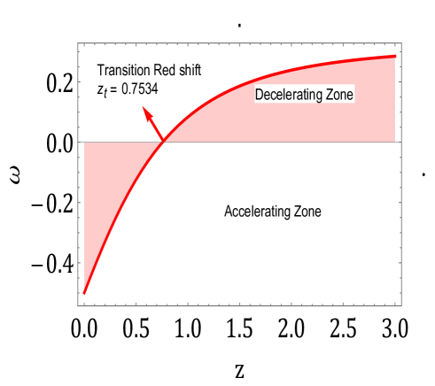
(a) (b)

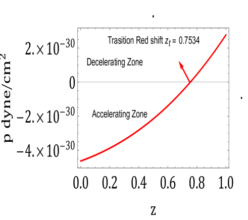
Figure 2: Figures (a) and (b) show the growth of equation of state parameter $\omega$ and pressure over red shift $`z^{\prime}$ respectively. It describes that in the past both the equation of state parameter $\omega$ and pressure were positive which means that universe was deceleration. At transition redshift $z_{t}$= 0.7534, where $\omega\sim 0~{}\&~{}p\sim 0$, they changed their behaviour and become negative which means that universe started accelerating at this junction. Here $\mu=130.$

We can also plot for density of the universe from Eq. (12). The following figure $3$ describes that in the past density was more. It gradually decreases due to expansion of the universe. As we describe earlier, $\rho_{0}$ is taken as $1.88\times 10^{-29}gm/cm^{3}$.

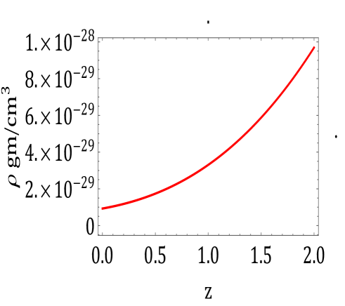
Figure 3: Figure describes the growth of density over red shift which is a increasing function. This means that in the past density was more. It gradually decreases due to expansion of the universe. Here $\mu=130.$

5 Energy Conditions

There are the three types of energy conditions [95] (a) Weak energy condition(WEC) $p+\rho\geq 0$ (b) Strong energy condition(SEC) $3p+\rho\geq 0$ and (c) Dominant energy condition(DEC) $\rho-p\geq 0$. Apart from these, the common condition in all the three is that the density should be positive (i.e. $\rho\geq 0$). The expressions for the above energy condition are as follows:

$$p(z)+\rho(z)=\text{$\rho$0}\frac{0.0145873\left(34.5254(z+1)^{2.96658}+1(z+1)^{0.034}\right)(z(z(z+3)+3)+3.55)^{0.978}}{(z+1)^{2.93258}+2.54909}$$ (26)

$$3~{}p(z)+\rho(z)=\text{$\rho$0}\frac{1.2644\left(-(z+1)^{0.034}+0.592556(z+1)^{2.96658}\right)(z(z(z+3)+3)+3.55)^{0.978}}{(z+1)^{2.93258}+2.54909}$$ (27)

and

$$\rho(z)-p(z)=\text{$\rho$0}\frac{1.29358\left(0.199473(z+1)^{2.96658}+1.(z+1)^{0.034}\right)(z(z(z+3)+3)+3.55)^{0.978}}{(z+1)^{2.93258}+2.54909}.$$ (28)

It is interesting that all the three conditions are being satisfied here despite negative pressure at present. It is more clear from the following figure $4$.

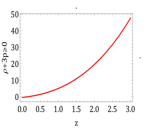
(a) (b) (c)

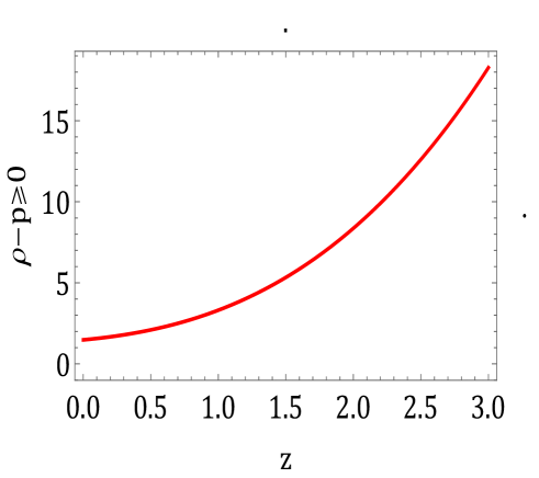
Figure 4: There are the three types of energy conditions (a) Weak energy condition $p+\rho\geq 0$ (b) Strong energy condition $3p+\rho\geq 0$ and (c) Dominant energy condition $\rho-p\geq 0$. It is interesting that all the three conditions are being satisfied here despite negative pressure at present. Here $\mu=130.$

6 Distant Modulus, Apparent Magnitude and Estimation of $H_{0}$ from their Data Set:

On the basis of the observations of some $42$ low red shift super nova’s, Supernova Cosmology Project and Supernova search team [ [4],[5]] headed by noble laureates S. Permutter and M. Riess, found that the distance modulus of these standard candles are more than what was predicted theoretically by standard FLRW model. There after, Some more data set such as Union 2.1 compilation [17], Pantheon Pan-STARRS1 data set [92] and more latest [93] $-$ [95] predict that due to higher values of distance modulus and apparent magnitudes of supernova’s, our universe is accelerating.
The distance modulus $\mu(z)$ is defined by [29]

$$\mu(z)=m_{b}-M=5LogD_{l}(z)+\mu_{0},$$ (29)

where $m_{b}$ and $M$ are the apparent and absolute magnitude of the standard candle respectively. The luminosity distance $D_{l}(z)$ and nuisance parameter $\mu_{0}$ are defined by

$$\mu_{0}=25+5Log\big{(}\frac{c}{H_{0}}\big{)},and$$ (30)

$$D_{l}(z)=(1+z)H_{0}\int_{0}^{z}{\frac{1}{H(z*)}dz*},$$ (31)

respectively.

In this section we will estimate present value of Hubble parameter $H_{0}$, from the two types of data set (a) $580$ distance modulus of supernova’s at the different red shift in the range $0\leq z\leq 1.5$ (b) $66$ Pantheon apparent magnitude $m_{b}$ data’s consisting of the latest compilation of SN Ia $40$ binned plus 26 high redshift data’s in the range $0.014\leq z\leq 2.26$.

6.1 Estimation by Data Set (a):

We compare the data set values from those obtained theoretically from Eqs. (29) $-$ (31) by forming the following chi squire functions of the present value of Hubble parameter $H_{0}$.

$$\chi^{2}(H_{0})=\frac{1}{579}\sum\limits_{i=1}^{580}\frac{[\mu th(z_{i},H_{0})-\mu ob(z_{i})]^{2}}{\sigma{(z_{i})}^{2}},$$ (32)

From Eq. (32), we find minimum $\chi^{2}$ for the set of $H_{0}$’s in the range (65$-$75). We obtain $\{H_{0}\to 69.7171\}\}$ for $\chi^{2}=\{0.97323\}$. This may be called a very good fit. The fit will be more clear from the following error bar and likelihood plots in the figure $6$.

Figure $6(a)$ describes the growth of distant modulus $\mu$ over red shift $`z^{\prime}$. The distant modulus is increasing function of red shift which means that in the past distant modulus was more. It is gradually decreasing over time. The figure also shows that theoretical graph passes near by through the dots which are observed values at different red shifts. Vertical lines are error bars. Figure $6(b)$ is likelihood probability curve for Hubble parameter. Estimated value $H_{0}=69.1434$ is at the peak.

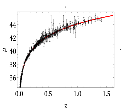
(a) (b)

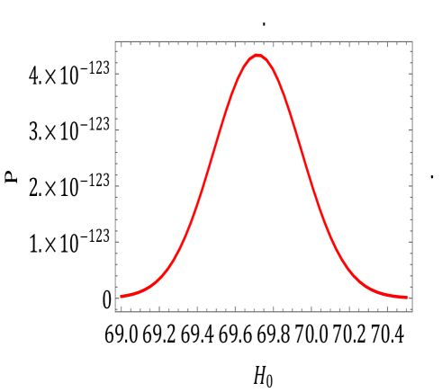
Figure 5: Figure (a) is the error bar plots for distant modulus $\mu$ over red shift $`z^{\prime}$. Figure (c) is likelihood probability curve for Hubble parameter. Estimated value $H_{0}=69.7171$ is at the peak.

6.2 Estimation by Data Set (b):

The data set (b) is comprised of 66 Pantheon apparent magnitude $m_{b}$ data’s in which $40$ are SN Ia binned and $26$ high redshift data’s in the range $0.014\leq z\leq 2.26$. The literature describes that the absolute magnitudes of a standard candles are more or less same. It is found [29] that the absolute magnitude of a supernova is obtained as $M=-19.09$, so we can convert all the apparent magnitude $m_{b}$ data’s into distant modulus data’s and vice-versa by adding or subtracting 19.09 into them. We may define expression for $m_{b}$ as follows:

$$m_{b}=5Log[(1+z)c\int_{0}^{z}{\frac{1}{H(z*)}dz*}]+5.91$$ (33)

We compare the data set values from those obtained theoretically from Eq. (33) by forming the following chi squire functions of the present value of Hubble parameter $H_{0}$.

$$\chi^{2}(H_{0})=\frac{1}{65}\sum\limits_{i=1}^{66}\frac{[m_{b}th(z_{i},H_{0})-m_{b}ob(z_{i})]^{2}}{\sigma{(z_{i})}^{2}},$$ (34)

From Eq. (34), we find minimum $\chi^{2}$ for the set of $H_{0}$’s in the range (65$-$75). We obtain $\{H_{0}\to 78.8906\}\}$ for $\chi^{2}=\{1.1144\}$. As it is nearer to one so it will also be called a good fit statistically. The fit will be more clear from the following error bar and livelihood plots in the figure $7$.

Figure $7(a)$ describes the growth of apparent magnitude $m_{b}$ over red shift $`z^{\prime}$. The apparent magnitude $m_{b}$ is increasing function of red shift which means that in the past distant modulus was more. It is gradually decreasing over time. The figure also shows that theoretical graph passes near by through the dots which are observed values at different red shifts. Vertical lines are error bars. Figure $7(b)$ is likelihood probability curve for Hubble parameter. Estimated value $H_{0}=78.8906$ is at the peak.

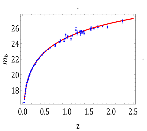
(a) (b)

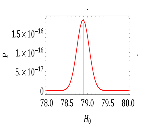
Figure 6: Figure (a) is the error bar plots for apparent magnitude $m_{b}$ over red shift $`z^{\prime}$. Figure (b) is likelihood probability curve for Hubble parameter. Estimated value $H_{0}=78.8906$ is at the peak.

7 Estimations of $H_{0}$ by combing the data sets:

In this section we will combine the various data sets used earlier. It is found that if we combine Hubble $46$ data set with data set (a), we get a data set of $657$ data’s. this gives the estimated value of $H_{0}$ as $H_{0}=69.367$ for minimum chi squire $\chi 2=0.864739$. Similarly on combining data set (a) and (b), we get a data set of 646 data’s. This gives the estimated value of $H_{0}$ as $H_{0}=78.5398$ for minimum chi squire $\chi 2=1.10473$. last if we combine all the three data sets, we get a data set of $657$ data’s. this gives the estimated value of $H_{0}$ as $H_{0}=77.914$ for $\chi 2=1.04471$. We present the following table to display all of our statistical findings.

7.1 Time versus Red Shift, Age of the Universe and Transitional times:

We can calculate the time of any event from the red shift through the following transformation

$$(t_{0}-t_{1})=\intop_{t_{1}}^{t_{0}}dt=\intop_{a_{1}}^{a_{0}}\frac{da}{aH}=\intop_{0}^{z_{1}}\frac{dz}{(1+z)H(z)},$$ (35)

where we have used $\frac{a_{0}}{a}=1+z$ and $\dot{z}=-(1+z)H.$ $t_{0}$ and $t_{1}$ are present and some past time. We note that at present,t=$t_{0}$ and z=0. With the help of expression for Hubble parameter Eq. (18), we can plot the graph of time versus red shift relation. This is given in following the figure $8$.
The figure $8$ describe time versus red shift transformation. There is a asymptote in the curve which gives the present age of the universe as $H_{0}t_{0}$= 0.9410. On the basis of the various estimates of $H_{0}$, the age of the universe comes to $13.5245*10^{9}$ yrs and $12.0854\times 10^{9}$ yrs in our model. The transition time where the universe inters the accelerating phase is also calculated as $4.10953\times 10^{9}$ yrs and $3.67228\times 10^{9}$ yrs as from now.

Table 1: Statistical estimations for Hubble parameter $H_{0}$

Datasets	$H_{0}$	$\chi^{2}$
$OHD$	$68.95$	$0.5378~{}$
D.M $\mu$	$69.7171$	$0.97323~{}$
A.M $m_{b}$	$78.8906$	$1.1144~{}$
$OHD$ + D.M $\mu$	$69.367$	$0.864739~{}$
D.M $\mu$ + A.M $m_{b}$	$78.5398$	$1.10473~{}$
$OHD$ + D.M $\mu$ + A.M $m_{b}$	$77.914$	$1.04471~{}$

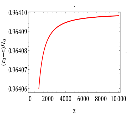
Figure 7: The figure describe time versus red shift transformation. There is a asymptote in the curve which gives the present age of the universe as $H_{0}t_{0}$= 0.9410.

8 Conclusion:

In a brief nutshell, we say that we have developed a FLRW type cosmological model of the universe in $f(R,T)$ gravity theory which deviates from its original features as per the needs of the present day observations. The main findings of our model are stated point wise.

• The model displays transition from deceleration in the past to the acceleration at the present. The three parameters namely the deceleration parameter $q$, pressure $p$ and equation of state parameter $\omega$ carries this transition.
  

• The interesting part in the paper is that the transition red shift is found similar in all the three parameters stated above in the item (i).

• Energy conditions in the model are evaluated and discussed. Interestingly, the model satisfies all the three weak, strong and Dominant energy conditions despite the presence of the negative pressure at present.

• We have considered the simplest form of $f(R,T)$ as $f(R,T)=R+\Lambda T$ and estimated $\mu=8\pi\lambda=130.$

• We will estimate present value of Hubble parameter $H_{0}$, from the three types of data set (a) 580 distance modulus of supernova’s at the different red shift in the range $0\leq z\leq 1.5$ (b) 66 Pantheon apparent magnitude $m_{b}$ data’s consisting of the latest compilation of SN Ia 40 binned plus $26$ high redshift data’s in the range $0.014\leq z\leq 2.26$ (c) latest compilation of $46$( OHD) observational Hubble data set.The out come of these is displayed in Table $1$.

• We have formulated apparent magnitude of a standard candle (see Eq. (31)).

• With the help of the various error bar plots and likelihood plots values of chi-squire, we tried to show how much our theoretical result tallies with the observational ones.

• We have calculated the age of the universe as per our model. one of the estimation is $13.5$ billion yrs. This value is at par with the observed one. Similarly we have also estimated Hubble constant at present as $68.95$ This value is also at par with the present observed values[20] $-$ [23].

• If we look at the table$-$ 1, we find that the present Hubble parameter has variations in its value on the basis of estimations by the three data sets and their combinations. It is observed that the $H_{0}\simeq 69$-$70$ for OHD and SNIa 580 distance modulus data, whereas when we use the pantheon data set, $H_{0}\simeq 78$-$79$. There is considerable difference in these values. We recall that we also face the same issue when we empirically find the present value of the Hubble parameter using calibrated distance ladder techniques and measurements of the cosmic microwave background. The former value comes to $H_{0}\simeq 73$ whereas the CMB based value is $H_{0}\simeq 68$. This is often given the name Hubble Tension.

The authors are confident that readers and researchers will find our work valuable in the final analysis.

References

- [1] Daniel Baumann, Cosmology (Cambridge University Press, 2022).
- [2] Matts Roos, Introduction to Cosmology (John Wiley & Sons Ltd, 2015).
- [3] J. V. Narlikar, Introduction to Cosmology (Cambridge University Press, 2002).
- [4] A. G. Riess, et al. [Supernova Search Team], Observational evidence from supernovae for an accelerating universe and a cosmological constant, Astron. J. 116 (1998) 1009-1038.
- [5] S. Perlmutter, et al. [Supernova Cosmology Project], Measurements of and from 42 high redshift supernovae, Astrophys. J. 517 (1999) 565-586.
- [6] S. Perlmutter, et al., Discovery of a supernova explosion at half the age of the Universe, Nature 391 (1998) 51.
- [7] J. L. Tonry, et al., Cosmological results from high-z supernovae, Astrophys. J. 594 (2003) 1.
- [8] A. Clocchiatti, et al., Hubble Space Telescope and ground-based observations of type Ia Supernovae at redshift 0:5: cosmological implications, Astrophys. J. 642, (2006) 1.
- [9] P. de Bernardis, et al., A flat universe from high-resolution maps of the cosmic microwave background radiation, Nature 404 (2000) 955-959.
- [10] S. Hanany, et al., MAXIMA-1: a measurement of the cosmic microwave background anisotropy on angular scales of 10’ 5, Astrophys. J. 545 L5L9 (2000).
- [11] D. N. Spergel, et al. [WMAP collaboration], First year wilkinson microwave anisotropy probe (WMAP) observations determination of cosmological parameters, Astrophys. J. Suppl. 148 (2003) 175.
- [12] M. Tegmark, et al. [SDSS collaboration], Cosmological parameters from SDSS and WMAP, Phys. Rev. D 69 (2004) 103501.
- [13] U. Seljak, et al., Cosmological parameter analysis including SDSS Ly forest and galaxy bias constraints on the primordial spectrum of fluctuations neutrino mass and dark energy, Phys. Rev. D 71 (2005) 103515.
- [14] J. K. Adelman-McCarthy, et al., The fourth data release of the sloan digital sky survey, Astrophys. J. Suppl. 162 (2006) 38.
- [15] C. L. Bennett, et al., First year wilkinson microwave anisotropy probe (WMAP) observations preliminary maps and basic results, The Astrophys. J. Suppl. 148 (2003) 1-43.
- [16] S. W. Allen, et al., Constraints on dark energy from chandra observations of the largest relaxed galaxy clusters, Mon. Not. R. Astron. Soc. 353 (2004) 457.
- [17] N. Suzuki, et al., The Hubble space telescope cluster supernova survey V improving the darkenergy constraints above z 1 and building an early-type-hosted supernova sample, Astrophys. J. 746 (2012) 85-115.
- [18] T. Delubac, et al. [BOSS Collaboration], 2015. Baryon acoustic oscillations in the Ly forest of BOSS DR11 quasars, Astron. Astrophys. 574 (2015) A59.
- [19] C. Blake, et al. [The Wiggle Z Dark Energy Survey], 2012. The Wiggle Z dark energy survey joint measurements of the expansion and growth history at , Mon. Not. R. Astron. Soc. 425 (2012) 405-414.
- [20] P. A. R. Ade, et al. [Planck Collaboration], 2016. Planck 2015 results XIV dark energy and modified gravity, Astron. Astrophys. 594 (2016) A14.
- [21] E. Komatsu, et al. [WMAP], Five-year wilkinson microwave anisotropy probe (WMAP) observations: Cosmological interpretation, Astrophys. J. Suppl. 180 (2009) 330-376.
- [22] E. Komatsu, et al., Seven-Year Wilkinson Microwave Anisotropy Probe (WMAP) Observations: Cosmological Interpretation, Astrophys. J. Suppl. 192 (2011) 18.
- [23] N. Aghanim et al., Planck 2018 results. VI. Cosmological parameters, Astron. Astrophys. 641 (2020) A6. [erratum: Astron. Astrophys. 652 (2021) C4.
- [24] S. Alam et al. (BOSS Collaboration), The clustering of galaxies in the completed SDSS-III Baryon Oscillation Spectroscopic Survey: cosmological analysis of the DR12 galaxy sample, Mon. Not. Roy. Astron. Soc. 470 (2017) 2617-2652.
- [25] M. M. Ivanov, Cosmological constraints from the power spectrum of eBOSS emission line galaxies, Phys. Rev. D 104 (2021) 103514.
- [26] T. Colas, G. D’amico, L. Senatore, P. Zhang, and F. Beutler, Efficient cosmological analysis of the SDSS/BOSS data from the effective field theory of large-scale structure, JCAP 2020(06) (2020) 001.
- [27] E. J. Copeland, M. Sami, and S. Tsujikawa, Dynamics of dark energy, Int. J. Mod. Phys. D 15 (2006) 1753-1936.
- [28] M. Li, X.-D. Li, S. Wang, and Y. Wang, Dark energy, Commun. Theor. Phys. 56 (2011) 525-604.
- [29] . Gron and S. Hervik, Einstein’s general theory of relativity with modern applications in cosmology (Springer Publication, 2007)
- [30] S. Weinberg,The cosmological constant problem, Rev. Mod. Phys. 61 (1989) 1.
- [31] P. J. E. Peebles and B. Ratra, The Cosmological constant and dark energy, Rev. Mod. Phys. 75 (2003) 559-606.
- [32] P. Steinhardt, L. Wang and I. Zlatev, Cosmological tracking solutions, Phys. Rev. D 59 (1999) 123504.
- [33] V. B. Johri, Genesis of cosmological tracker fields, Phys. Rev. D 63 (2001) 103504.
- [34] R. R.Caldwell, A phantom menace? Cosmological consequences of a dark energy component with super-negative equation of state, Phys. Lett. B 545 (2002) 23-29.
- [35] V. B. Johri, Phantom cosmologies, Phys. Rev. D 70 (2004) 041303.
- [36] Y. Gong and Y. Zhang, Probing the curvature and dark energy, Phys. Rev. D 72 (2005) 043518.
- [37] D. Huterer and M.S. Turner, Probing dark energy: Methods and strategies, Phys. Rev. D 64 (2001) 123527.
- [38] J. Weller and A. Albrecht, Future supernovae observations as a probe of dark energy, Phys. Rev. D 65 (2002) 103512.
- [39] M. Chevallier and D. Polarski, Accelerating universes with scaling dark matter, Int. J. Mod. Phys. D 10 (2001) 213-223.
- [40] T. Roy Choudhary and T. Padmanabhan, Cosmological parameters from supernova observations: A critical comparison of three data sets, Astron. Astrophys. 429 (2005) 807.
- [41] H. K. Jassal, J. S. Bagla and T. Padmanabhan, WMAP constraints on low redshift evolution of dark energy, Monthly Not. Roy. Astron. Soci.: Lett. 356 (2005) L11-L16.
- [42] T. Padmanabhan and T. Roy Choudhury, A theoretician’s analysis of the supernova data and the limitations in determining the nature of dark energy, Monthly Not. Roy. Astron. Soci. 344 (2003) 823-834.
- [43] H. Motohashi, A. A. Starobinsky, and J. Yokoyama, gravity and its cosmological implications, Int. J. Mod. Phys. D 20 (2011) 1347-1355.
- [44] A. S. Agrawal, Francisco Tello-Ortiz, B. Mishra, and A. Alvarez, f(R) wormholes embedded in pseudo-Euclidean space E5, Fortschritte der Physik 70 (2022) 2100177.
- [45] S. A. Narawade, L. Pati, B. Mishra, and S. K. Tripathy, Dynamical system analysis for accelerating models in non-metricity gravity, Phys. Dark Univ. 36 (2022) 101020.
- [46] M. Koussour, S. H. Shekh, M. Govender, and M. Bennai, Thermodynamical aspects of Bianchi type-I universe in quadratic form of gravity and observational constraints, J. High Energy Astrophys, 37 (2022) 15.
- [47] J. Frieman, M. Turner, and D. Huterer, Dark energy and the accelerating universe, Ann. Rev. Astron. Astrophys. 46 (2008) 385-432.
- [48] S. Nojiri and S. D. Odintsov, Introduction to modified gravity and gravitational alternative for dark energy, eConf C0602061 (2006) 06, [arXiv:hep-th/0601213].
- [49] Santosh V. Lohakare, S. K. Tripathy, and B. Mishra, Cosmological model with time varying deceleration parameter in gravity, Physica Scripta 96 (2021) 125039.
- [50] F. S. N. Lobo, The Dark side of gravity: Modified theories of gravity, arXiv preprint arXiv:0807.1640.
- [51] S. Capozziello and M. Francaviglia, Extended theories of gravity and their cosmological and astrophysical applications, Gen. Rel. Grav. 40 (2008) 357-420.
- [52] S. Nojiri, S. D. Odintsov, and O. G. Gorbunova, Dark energy problem: from phantom theory to modified Gauss-Bonnet gravity, Journal of Physics A: Mathematical General, 39 (2006) 6627.
- [53] A. Chudaykin, K. Dolgikh, and M. M. Ivanov, Constraints on the curvature of the universe and dynamical dark energy from the full-shape and BAO data, Phys. Rev. D 103 (2021) 023507.
- [54] T. Harko, F. S. N. Lobo, S. Nojiri, and S. D. Odintsov, gravity, Phys. Rev. D 84 (2011) 024020.
- [55] S. B. Fisher and E.D. Carlson, Reexamining gravity, Phys. Rev. D 100 (2019) 064059.
- [56] T. Harko and P. H. R. S. Moraes, Comment on Reexamining gravity, Phys. Rev. D 101 (2020) 108501.
- [57] A. K. Yadav, P. K. Sahoo, and V. Bhardwaj, Bulk viscus Bianchi-I embedded cosmological model in gravity, Mod. Phys. Lett. A 34 (2019) 1950145.
- [58] L. K. Sharma, B. K. Singh, and A. K. Yadav, Viability of Bianchi type universe in gravity, Int. J. Geom. Methods Mod. Phys. 17 (2020) 2050111.
- [59] U. K. Sharma, M. Kumar, and G. Varshney, Scalar field models of Barrow holographic dark energy in gravity, Universe 12(8) (2022) 642.
- [60] B. Mishra, F. M. D. Esmaeili, and S. Ray: Cosmological model with variable anisotropic parameter in gravity, Indian Jour. Phys. 95 (2021) 2245.
- [61] V. K. Bhardwaj and A. Pradhan, Evaluation of cosmological models in gravity in different dark energy scenario, New Astronomy 91 (2022) 101675.
- [62] G. G. L. Nashed, S. D. Odintsov, and V. K. Oikonomou, Anisotropic compact stars in D-4 limits of Gauss-Bonnet-Gravity, Symmetry 14(3) (2022) 545.
- [63] T. Tangphati, S. Hansraj, A. Banerjee, and A. Pradhan, Quark stars gravity with an interacting quark equation of state, Phys. Dark Univ. 35 (2022) 100990.
- [64] J. M. Z. Pretel, T. Tangphati, A. Banerjee, and A. Pradhan, Charged quark stars in gravity, Chin. Phys. C 46 (2022) 115103.
- [65] K. Bamba, S. Capozziello, S. Nojiri and S. D. Odintsov, Dark energy cosmology: the equivalent description via different theoretical models and cosmography tests, Astrophys. Space Sci. 342 (2012) 155.
- [66] S. Nojiri and S. D. Odintsov, Unified cosmic history in modified gravity: from theory to Lorentz non-invariant models, Phys. Rept. 505 (2011) 59-144.
- [67] A. Pradhan, A. Dixit, and D. C. Maurya, Quintessence, behaviour of an anisotropic bulk viscous cosmological model in modified gravity, Symmetry 14(12) (2022) 2630.
- [68] S. Capozziello and R. D’Agostino, Model-independent reconstruction of non-metric gravity. Phys. Lett. B 832 (2022) 137229.
- [69] I. Ayuso, R. Lazkoz, and V. Salzano, Observational constraints on cosmological solutions of theories, Phys. Rev. D 103 (2021) 063505.
- [70] G. N. Gadbail, S. Mandal, and P. K. Sahoo, Parametrization of deceleration parameter in gravity, Physics 4(4) (2022) 1403.
- [71] L. Pati, B. Mishra, S. K. Tripathy: Model parameters in the context of late time cosmic acceleration in gravity, Physica Scripta 96 (2021) 105003.
- [72] V. Zhong and D. S.-C. Gomez, Inflation in mimetic gravity, Symmetry 10(5) (2018) 170.
- [73] A. Dixit and A. Pradhan, Bulk viscous flat FLRW model with observational constraints in gravity, Universe 8(12) (2022) 650.
- [74] S. H. Shekh, V. R. Chirde, and P. K. Sahoo, Energy conditions of the gravity dark energy model with the validity of thermodynamics, Comm. Theor. Phys. 22 (2020) 085402.
- [75] S. Bahamonde and S. Capozziello, Noether symmetry approach in teleparallel cosmology, Eur. Phys. J. C 77 (2017) 1–10.
- [76] S. Nojiri, S. D. Odintsov and V. K. Oikonomou, Modified Gravity Theories on a Nutshell: Inflation, Bounce and Late-time Evolution, Phys. Rept. 692 (2017) 1-104.
- [77] E. Macaulay, et al. [DES], First cosmological results using Type Ia supernovae from the dark energy survey: Measurement of the Hubble constant, Mon. Not. Roy. Astron. Soc. 486 (2019) 2184-2196.
- [78] C. Zhang, H. Zhang, S. Yuan, T. J. Zhang and Y. C. Sun, four new observational data from luminous red galaxies in the sloan digital sky Survey data release seven, Res. Astron. Astrophys. 14 (2014) 1221-1233.
- [79] D. Stern, R. Jimenez, L. Verde, M. Kamionkowski, SA. Stanford, Cosmic chronometers: constraining the equation of state of dark energy. I: measurements, JCAP 2010(02) (2010) 008.
- [80] E. Gaztanaga, A. Cabre and L. Hui, Clustering of luminous red galaxies IV: Baryon acoustic peak in the line-of-sight direction and a direct measurement of , Mon. Not. Roy. Astron. Soc. 399 (2009) 1663-1680.
- [81] C. H. Chuang and Y. Wang, Modeling the anisotropic two-point galaxy correlation Function on Small Scales and Improved Measurements of , , and from the Sloan Digital Sky Survey DR7 Luminous Red Galaxies, Mon. Not. Roy. Astron. Soc. 435 (2013) 255-262.
- [82] S. Alam et al. [BOSS], The clustering of galaxies in the completed SDSS-III baryon oscillation spectroscopic survey: cosmological analysis of the DR12 galaxy sample, Mon. Not. Roy. Astron. Soc. 470 (2017) 2617-2652.
- [83] C. Blake, S. Brough, M. Colless, C. Contreras, W. Couch, S. Croom, D. Croton, T. Davis, M. J. Drinkwater and K. Forster, et al. The WiggleZ dark energy survey: Joint measurements of the expansion and growth history at z 1, Mon. Not. Roy. Astron. Soc. 425 (2012) 405-414.
- [84] A. L. Ratsimbazafy, S. I. Loubser, S. M. Crawford, C. M. Cress, B. A. Bassett, R. C. Nichol and P. Väisänen, Age-dating luminous red galaxies observed with the Southern African large telescope, Mon. Not. Roy. Astron. Soc. 467 (2017) 3239-3254.
- [85] M. Moresco, Raising the bar: new constraints on the Hubble parameter with cosmic chronometers at , Mont. Not. Royal Astron. Soci. Lett. 450 (2015) L16-L20.
- [86] J. Simon, L. Verde, and R. Jimenez, Constraints on the redshift dependence of the dark energy potential, Phys. Rev. D 71 (2005) 123001.
- [87] M. Moresco, et al. Improved constraints on the expansion rate of the universe up to from the spectroscopic evolution of cosmic chronometers, JCAP 2012(08) (2012) 006.
- [88] M. Moresco, et al. A 6 measurement of the Hubble parameter at direct evidence of the epoch of cosmic re-acceleration, JCAP 2016(05) (2016) 014.
- [89] T. Delubac, J. Rich, S. Bailey, A. Font-Ribera, et al., Baryon acoustic oscillations in the Ly forest of BOSS quasars, Astron. Astrophys. 552 (2013) A96.
- [90] T. Delubac, J. E. Bautista, J. Rich, D. Kirkby, et al. Baryon acoustic oscillations in the Ly forest of BOSS DR11 quasars, Astron. Astrophys. 574 (2015) A59.
- [91] A. Font-Ribera, et al., Quasar-Lyman forest cross-correlation from BOSS DR11: Baryon acoustic oscillations, JCAP 2014(05) (2014) 027.
- [92] M. Visser, Energy conditions in the epoch of galaxy formation, Science 276 (1997) 88-90.
- [93] D. M. Scolnic et al. [Pan-STARRS1], The complete Light-curve sample of spectroscopically confirmed SNe Ia from Pan-STARRS1 and cosmological constraints from the combined Pantheon sample, Astrophys. J. 859 (2018) 101.
- [94] D. Scolnic, D. Brout, A. Carr, A. G. Riess, T. M. Davis, A. Dwomoh, D. O. Jones, N. Ali, P. Charvu and R. Chen, et al. The Pantheon+ Analysis: The Full Data Set and Light-curve Release, Astrophys. J. 938 113 (2022).
- [95] D. Brout, D. Scolnic, B. Popovic, A. G. Riess, J. Zuntz, R. Kessler, A. Carr, T. M. Davis, S. Hinton and D. Jones, et al.‘The Pantheon+ Analysis: Cosmological Constraints, Astrophys. J. 938 110 (2022).