Shannon entropy in quasiparticle states of quantum chains

Abstract

In this paper, we investigate the Shannon entropy of the total system and its subsystems, as well as the subsystem Shannon mutual information, in quasiparticle excited states of free bosonic and fermionic chains and the ferromagnetic phase of the spin-1/2 XXX chain. Our focus is on single-particle and double-particle states, and we derive various analytical formulas for free bosonic and fermionic chains in the scaling limit. These formulas are also applicable to magnon excited states in the XXX chain under certain conditions. We discover that, unlike entanglement entropy, Shannon entropy does not separate when two quasiparticles have a large momentum difference. Moreover, in the large momentum difference limit, we obtain universal results for quantum spin chains that cannot be explained by a semiclassical picture of quasiparticles.

¹Department of Physics, School of Science, Tianjin University,
135 Yaguan Road, Tianjin 300350, China
²Center for Joint Quantum Studies, School of Science, Tianjin University,
135 Yaguan Road, Tianjin 300350, China

1 Introduction

In quantum mechanics, one can express the state of a quantum system in a pure state $|\psi\rangle$ in any orthonormal basis $\{|i\rangle\}$ with $\langle i|j\rangle=\delta_{ij}$ as

$$|\psi\rangle=\sum_{i}c_{i}|i\rangle,$$ (1.1)

where the normalization of the state $\langle\psi|\psi\rangle=1$ implies that $\{p_{i}=|c_{i}|^{2}\}$ forms a well-defined probability distribution, i.e., $p_{i}\geq 0$ and $\sum_{i}p_{i}=1$. A quantum system in a mixed state is characterized by a density matrix $\rho$, which is positive semi-definite and satisfies $\textrm{tr}\rho=1$. One can write the density matrix in the orthonormal basis $\{|i\rangle\}$ as

$$\rho=\sum_{i,j}\rho_{ij}|i\rangle\langle j|,$$ (1.2)

and there is a well-defined probability distribution $\{p_{i}=\rho_{ii}\}$. The Shannon entropy [1, 2]

$$H=-\sum_{i}p_{i}\log p_{i},$$ (1.3)

can be calculated for any arbitrary probability distribution $\{p_{i}\}$, which measures the uncertainty or randomness of the probability distribution. In the case of a quantum system in a pure or mixed state, the Shannon entropy depends on the chosen basis. In quantum spin chains, the direct product of the local basis at each individual site forms a natural basis. In the local basis, the Shannon entropy characterizes a type of interesting correlation between different parts of the quantum system. The Shannon entropy in the local basis of various quantum spin chains has been intensively studied for both the total system [3, 4, 5, 6, 7, 8, 9] and a subsystem [10, 11, 12, 13, 14, 15, 16, 17, 18, 19]. The probabilities of finding different states in this basis are called formation probabilities [17]. These probabilities, especially the empty formation probability, have been the subject of extensive research [20, 21, 22, 23, 24, 25, 26, 5, 11, 17, 27, 28, 29, 30, 31, 32].

Typically, in numerous studies, the entire system is assumed to be in its ground state, while a subsystem is often in a mixed state. In this paper, we examine the Shannon entropy of both the entire system and a connected subsystem in states of quasiparticle excitations of free bosonic and fermionic chains and the spin-1/2 XXX chain. The results are then compared across diverse quantum spin chains and also with classical results. As depicted in Figure 1, we consider a connected subsystem $A=[1,\ell]$ with $\ell$ neighboring sites on a circular chain consisting of $L$ sites. Only translation-invariant states in quantum spin chains and translation-invariant configurations in classical chains are taken into account. We compute the Shannon entropy of the entire system $H(L)$ and the subsystem Shannon entropy $H(\ell)$. Additionally, we evaluate the subsystem Shannon mutual information,

$$M(\ell)=H(\ell)+H(L-\ell)-H(L),$$ (1.4)

which is a measure of the correlation between the subsystem $A$ and its complement $B$. Our focus is on understanding the behaviours in the total system Shannon entropy $H(L)$, the subsystem Shannon entropy $H(\ell)$, and the subsystem mutual information $I(\ell)$ as we approach the scaling limit $L\to+\infty$, $\ell\to+\infty$ while maintaining a constant ratio $x=\ell/L$.

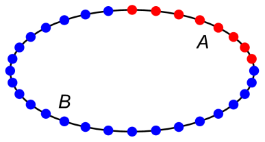
Figure 1: The spin chain consists of $L$ sites arranged in a circle. We consider a connected subsystem $A$ with $\ell$ adjacent sites, defined as $A=[1,\ell]$, and its complement $B=[\ell+1,L]$.

The aim of this paper is to investigate whether there exist universal properties for the total system Shannon entropy, subsystem Shannon entropy, and subsystem Shannon mutual information in excited states of quasiparticles, akin to those observed for entanglement entropy. In a state that is pure, the quantum correlation between a subsystem and its complement is usually described by the entanglement entropy, which refers to the von Neumann entropy of the reduced density matrix. Depending on the particular quantum state of a given many-body system, the entanglement entropy exhibits various behaviors in the scaling limit [33, 34, 35, 36, 37]. In specific scenarios, the entanglement entropy in quasiparticle states of integrable quantum spin chains displays intriguing universal features in the scaling limit [38, 39, 40, 41, 42, 43, 44, 45, 46, 47, 48, 49, 50, 51, 52, 53]. A quasiparticle state could be represented by the momenta $K$ of the excited quasiparticles, denoted as $|K\rangle$. The reduced density matrix of subsystem $A$ can be denoted as $\rho_{A}$, and the entanglement entropy can be calculated as $S_{A,K}=-\textrm{tr}_{A}(\rho_{A}\log\rho_{A})$. It has been discovered that under the large energy condition

$$\max_{k\in K}\frac{1}{\varepsilon_{k}}\ll\min(\ell,L-\ell),$$ (1.5)

where $\varepsilon_{k}$ is energy of the elementary excitation of one quasiparticle with momentum $k$, and the large momentum difference condition

$$|k-k^{\prime}|\gg 1,~{}\forall k\in K,\forall k^{\prime}\in K^{\prime},$$ (1.6)

the entanglement entropy difference is given by [49]

$$S_{A,K\cup K^{\prime}}-S_{A,K^{\prime}}=-\textrm{tr}_{A}(\tilde{\rho}_{A,K}\log\tilde{\rho}_{A,K}),$$ (1.7)

where $\tilde{\rho}_{A,K}$ is an effective low-rank reduced density matrix. In other words, under the conditions (1.5) and (1.6), the spin chain with modes $K^{\prime}$ acts like a background, and contributions from the modes $K$ to the entanglement entropy decouple from the background. Analytical formulas of the entanglement entropy difference in free bosonic and fermionic chains were obtained in [46, 47, 49], and these formulas and their proper combinations also apply to models with interactions such as spin-1/2 XXX chain and XXZ chain under certain conditions [49]. Furthermore, under the extra large momentum difference condition [46, 47]

$$|k_{1}-k_{2}|\gg 1,~{}\forall k_{1},k_{2}\in K,k_{1}\neq k_{2},$$ (1.8)

the effective reduced density matrix $\tilde{\rho}_{A,K}$ has a simple semiclassical quasiparticle picture and the entanglement entropy difference (1.7) becomes the Shannon entropy of the probability distribution of the semiclassical quasiparticles [41, 42]. It was found recently that similar universal properties and semiclassical quasiparticle picture also apply to the subsystem distance in quasiparticle excited states of various quantum spin chains [45, 48, 54].

In this paper, we present analytical formulas for the total and subsystem Shannon entropy and mutual information in single- and double-quasiparticle excited states of free bosonic and fermionic chains, as well as in single- and double-magnon excited states of the ferromagnetic phase of the spin-1/2 XXX chain. In the scaling limit where $L$ and $\ell$ approach infinity with a fixed ratio between subsystem size and total system size $x={\ell}/{L}$, both the total system Shannon entropy and subsystem Shannon entropy follow a logarithmic law, while the subsystem mutual information is a finite function of the ratio $x$. The results obtained for free bosonic and fermionic chains can also be applied to the XXX chain under certain circumstances. We compare our results with those of classical particles. In a single-particle state, the results are trivial and universal. In a double-particle state with a large momentum difference, we derive universal formulas that apply to all three types of quantum chains but cannot be reproduced semiclassically. In the scaling limit, the contributions from different classical particles decouple, whereas this is not the case for quantum quasiparticles, even in the large momentum difference limit.

The rest of this paper is organized in the following way. In sections 2 and 3, we present calculations of the total system Shannon entropy and subsystem Shannon entropy and mutual information in quasiparticle excited states in free bosonic and fermionic chains, respectively. In section 4, we consider magnon excited states in the spin-1/2 XXX chain. The paper concludes with discussions in section 5. In appendix A, we consider the configurations of classical particles. In appendix B, we calculate the Shannon entropy for the probability distribution of subsystem particle numbers in free bosonic and fermionic chains. Finally, in appendix C, we study the Shannon entropy in the local basis of $\sigma_{j}^{x}$ eigenstates of the XXX chain.

2 Free bosonic chain

In this section, we evaluate the total system and subsystem Shannon entropies and mutual information for the free bosonic chain in the single-particle state $|k\rangle$ and the double-particle states $|k^{2}\rangle$ and $|k_{1}k_{2}\rangle$.

2.1 Quasiparticle excited states

The free bosonic chain has the Hamiltonian

$$H=\sum_{j=1}^{L}\Big{(}a_{j}^{\dagger}a_{j}+\frac{1}{2}\Big{)}.$$ (2.1)

We define the global modes

$$b_{k}^{\dagger}\equiv\frac{1}{\sqrt{L}}\sum_{j=1}^{L}\mathrm{e}^{\frac{2\pi\mathrm{i}jk}{L}}a_{j}^{\dagger},~{}b_{k}\equiv\frac{1}{\sqrt{L}}\sum_{j=1}^{L}\mathrm{e}^{-\frac{2\pi\mathrm{i}jk}{L}}a_{j},~{}k=1,2,\cdots,L.$$ (2.2)

The ground state is defined as

$$a_{j}|G\rangle=b_{k}|G\rangle=0,~{}\forall j,\forall k.$$ (2.3)

Using the global modes $b_{k}^{\dagger}$, one could construct the general translation-invariant global state

$$|k_{1}^{r_{1}}k_{2}^{r_{2}}\cdots k_{s}^{r_{s}}\rangle=\frac{(b^{\dagger}_{k_{1}})^{r_{1}}(b^{\dagger}_{k_{2}})^{r_{2}}\cdots(b^{\dagger}_{k_{s}})^{r_{s}}}{\sqrt{r_{1}!r_{2}!\cdots r_{s}!}}|G\rangle.$$ (2.4)

In the free bosonic chain, the natural local basis at each site is the eigenstates of the operator of the excitation number. One could use the local modes $a_{j}^{\dagger}$ to construct the general locally excited state

$$|j_{1}^{r_{1}}j_{2}^{r_{2}}\cdots j_{s}^{r_{s}}\rangle=\frac{(a^{\dagger}_{j_{1}})^{r_{1}}(a^{\dagger}_{j_{2}})^{r_{2}}\cdots(a^{\dagger}_{j_{s}})^{r_{s}}}{\sqrt{r_{1}!r_{2}!\cdots r_{s}!}}|G\rangle,$$ (2.5)

which we will call local state for short. In the Hilbert space of the subsystem $A=[1,\ell]$, one has similarly the subsystem ground state $|G\rangle_{A}$ defined as

$$a_{j}|G\rangle_{A}=0,~{}\forall j\in A,$$ (2.6)

as well as the subsystem local excited states

$$|j_{1}^{r_{1}}j_{2}^{r_{2}}\cdots j_{s}^{r_{s}}\rangle_{A}=\frac{(a^{\dagger}_{j_{1}})^{r_{1}}(a^{\dagger}_{j_{2}})^{r_{2}}\cdots(a^{\dagger}_{j_{s}})^{r_{s}}}{\sqrt{r_{1}!r_{2}!\cdots r_{s}!}}|G\rangle_{A},~{}j_{1},j_{2},\cdots,j_{s}\in A.$$ (2.7)

2.2 Single-particle state $|k\rangle$

We first consider the global single-particle state $|k\rangle=b_{k}^{\dagger}|G\rangle$, which could be written in terms of local states as

$$|k\rangle=\frac{1}{\sqrt{L}}\sum_{j=1}^{L}\mathrm{e}^{\frac{2\pi\mathrm{i}jk}{L}}|j\rangle.$$ (2.8)

In state $|k\rangle$, there are $L$ possible local states $|j\rangle$ with $j\in[1,L]$, and the corresponding probabilities are

$$p_{j}=\frac{1}{L},~{}j\in[1,L].$$ (2.9)

We get the Shannon entropy

$$H^{\textrm{bos}}_{k}(L)=\log L.$$ (2.10)

For the subsystem $A$, there are $\ell+1$ possible local states and the corresponding probabilities are listed in Table 1. We get the Shannon entropy

$$H^{\textrm{bos}}_{k}(\ell)=x\log L-(1-x)\log(1-x),$$ (2.11)

and the Shannon mutual information

$$I_{k}^{\textrm{bos}}(\ell)=-x\log x-(1-x)\log(1-x).$$ (2.12)

local states	probabilities	ranges	numbers
$|G\rangle_{A}$	$p_{0}=1-x$	-	1
$|j\rangle_{A}$	$p_{j}=\frac{1}{L}$	$j\in[1,\ell]$	$\ell$

Table 1: The local states and probabilities of the subsystem $A$ in the single particle state $|k\rangle$ of the free bosonic chain.

The results for the single-particle state $|k\rangle$ are the same with the results for the configuration of one classical particle (A.19), (A.20) and (A.21).

2.3 Double-particle state $|k^{2}\rangle$

In terms of the local states, the global double-particle state $|k^{2}\rangle=\frac{1}{\sqrt{2}}(b_{k}^{\dagger})^{2}|G\rangle$ could be written as

$$|k^{2}\rangle=\frac{1}{L}\sum_{j=1}^{L}\mathrm{e}^{\frac{4\pi ijk}{L}}|j^{2}\rangle+\frac{\sqrt{2}}{L}\sum_{1\leq j_{1}<j_{2}\leq L}e^{\frac{2\pi ik(j_{1}+j_{2})}{L}}|j_{1}j_{2}\rangle.$$ (2.13)

There are $\frac{L(L+1)}{2}$ possible local states, and the probabilities are shown in Table 2, which are the same as the probabilities of the configuration of two identical classical soft-core in Table 8. In the limit $L\to+\infty$, we get the Shannon entropy

$$H^{\textrm{bos}}_{k^{2}}(L)=2\log L-\log 2.$$ (2.14)

local states	probabilities	ranges	numbers
$|j^{2}\rangle$	$p_{j^{2}}=\frac{1}{L^{2}}$	$j\in[1,L]$	$L$
$|j_{1}j_{2}\rangle$	$p_{j_{1}j_{2}}=\frac{2}{L^{2}}$	$1\leq j_{1}<j_{2}\leq L$	$\frac{L(L-1)}{2}$

Table 2: The local states and probabilities of the total system in the double-particle state $|k^{2}\rangle$ of the free bosonic chain.

For the subsystem $A$, there are $\frac{(\ell+1)(\ell+2)}{2}$ possible local states and the corresponding probabilities are shown in Table 3. In the scaling limit, we get the Shannon entropy

$$H^{\textrm{bos}}_{k^{2}}(\ell)=2x\log L-x(2-x)\log 2-2(1-x)\log(1-x),$$ (2.15)

and mutual information

$$I_{k^{2}}^{\textrm{bos}}(\ell)=-x^{2}\log x^{2}-2x(1-x)\log[2x(1-x)]-(1-x)^{2}\log(1-x)^{2}.$$ (2.16)

local states	probabilities	ranges	numbers
$|G\rangle_{A}$	$p_{0}=(1-x)^{2}$	-	1
$|j\rangle_{A}$	$p_{j}=\frac{2(1-x)}{L}$	$j\in[1,\ell]$	$\ell$
$|j^{2}\rangle_{A}$	$p_{j^{2}}=\frac{1}{L^{2}}$	$j\in[1,\ell]$	$\ell$
$|j_{1}j_{2}\rangle_{A}$	$p_{j_{1}j_{2}}=\frac{2}{L^{2}}$	$1\leq j_{1}<j_{2}\leq\ell$	$\frac{\ell(\ell-1)}{2}$

Table 3: The local states and probabilities of the subsystem $A$ in the double-particle state $|k^{2}\rangle$ of the free bosonic chain.

The results for the double-particle state $|k^{2}\rangle$ are the same as the results for the configuration of two identical classical particles (A.22), (A.23), and (A.24). It is easy to check that the results in the general $r$-particle state $|k^{r}\rangle=\frac{1}{\sqrt{r!}}(b_{k}^{\dagger})^{r}|G\rangle$ are the same as the results for the configuration of $r$ identical classical particles (A.28), (A.29), and (A.30). We skip the details of the calculation in this paper.

2.4 Double-particle state $|k_{1}k_{2}\rangle$

In this subsection we calculate the Shannon entropy for the double-particle state $|k_{1}k_{2}\rangle=b^{\dagger}_{k_{1}}b^{\dagger}_{k_{2}}|G\rangle$ in free bosonic chain.

2.4.1 Total system Shannon entropy

The double-particle state $|k_{1}k_{2}\rangle$ could be written in terms of local states as

$$|k_{1}k_{2}\rangle=\frac{\sqrt{2}}{L}\sum_{j=1}^{L}e^{\frac{2\pi\mathrm{i}j(k_{1}+k_{2})}{L}}|j^{2}\rangle+\frac{2}{L}\sum_{1\leq j_{1}<j_{2}\leq L}e^{\frac{\pi\mathrm{i}}{L}(j_{1}+j_{2})(k_{1}+k_{2})}\cos\frac{\pi j_{12}k_{12}}{L}|j_{1}j_{2}\rangle,$$ (2.17)

with the shorthand $j_{12}\equiv j_{1}-j_{2}$ and $k_{12}\equiv k_{1}-k_{2}$. As there is period $L$ for the momentum $k\cong k+L$, we only need to consider the case with $1\leq|k_{12}|\leq\frac{L}{2}$. There are $\frac{L(L+1)}{2}$ possible local states, and the probabilities are shown in Table 4. For general $L$ and $k_{12}$, we get the Shannon entropy of the total system

$$H^{\textrm{bos}}_{k_{1}k_{2}}(L)=2\log L-2\log 2+\frac{2\log 2}{L}-\frac{4}{L}\sum_{j=1}^{L/2-1}\cos^{2}\frac{\pi jk_{12}}{L}\log\cos^{2}\frac{\pi jk_{12}}{L}.$$ (2.18)

For $|k_{12}|\ll L$ in the limit $L\to+\infty$, the Shannon entropy becomes

$$H^{\textrm{bos}}_{k_{1}k_{2}}(L)=2\log L-1,$$ (2.19)

which does not depend on the actual values of the momenta $k_{1},k_{2}$. As we will see in the subsequent section, the formula (2.19) also applies to the free fermionic chain under the condition $|k_{12}|\ll L$. We also call it a universal result

$$H^{\textrm{univ}}_{k_{1}k_{2}}(L)=2\log L-1.$$ (2.20)

local states	probabilities	ranges	numbers
$|j^{2}\rangle$	$p_{j^{2}}=\frac{2}{L^{2}}$	$j\in[1,L]$	$L$
$|j_{1}j_{2}\rangle$	$p_{j_{1}j_{2}}=\frac{4}{L^{2}}\cos^{2}\frac{\pi j_{12}k_{12}}{L}$	$1\leq j_{1}<j_{2}\leq L$	$\frac{L(L-1)}{2}$

Table 4: The local states and probabilities of the total system in the double-particle state $|k_{1}k_{2}\rangle$ of the free bosonic chain.

When $|k_{12}|$ is proportional to $L$ in the scaling limit $L\to+\infty$, the Shannon entropy may take exceptional values for exceptional values of $|k_{12}|$. For $|k_{12}|=\frac{mL}{n}\leq\frac{L}{2}$ with the integer $n=2,3,4,\cdots$ being a divider of $L$ and the integer $m$ being coprime with $n$, we get the total system Shannon entropy

$$\mathcal{H}^{\textrm{bos}}_{k_{1}k_{2}}(L)=2\log L-2\log 2-\frac{2}{n}\sum_{a=1}^{n-1}\cos^{2}\frac{\pi a}{n}\log\cos^{2}\frac{\pi a}{n},$$ (2.21)

which is independent of $m$. Explicitly, for $n=\{2,3,4,5,6\}$, we get respectively

$$\mathcal{H}^{\textrm{bos}}_{k_{1}k_{2}}(L)-2\log L=\Big{\{}-2\log 2,-\frac{4}{3}\log 2,-\frac{3}{2}\log 2,$$

$$\phantom{\mathcal{H}^{\textrm{bos}}_{k_{1}k_{2}}(L)-2\log L=}-\frac{1}{5}\log 2-\frac{1}{10}[(3-\sqrt{5})\log(3-\sqrt{5})+(3+\sqrt{5})\log(3+\sqrt{5})],$$

$$\phantom{\mathcal{H}^{\textrm{bos}}_{k_{1}k_{2}}(L)-2\log L=}-\frac{2}{3}\log 2-\frac{1}{2}\log 3\Big{\}}.$$ (2.22)

For $n=5$, we may have either $m=1$ or $m=2$, and the Shannon entropy $\mathcal{H}^{\textrm{bos}}_{k_{1}k_{2}}(L)$ does not depend on $m$. For a prime integer $L$, there is no $|k_{12}|=\frac{mL}{n}\leq\frac{L}{2}$ with coprime integers $m,n$, and so the formula (2.19) is valid for all $k_{12}$ for a large prime integer $L$. Interestingly, in further $n\to+\infty$ limit, the exceptional formula (2.21) approaches the universal formula (2.20).

We have obtained three formulas for the total system Shannon entropy, i.e. the exact formula (2.18) written in terms of a summation which is valid for general $L$ and $k_{12}$, the formula (2.19), i.e. the universal formula (2.20), which is valid for $|k_{12}|\ll L$ in the scaling limit, and the exceptional formula (2.21) which is valid for exceptional values of the momentum difference $|k_{12}|=\frac{mL}{n}\leq\frac{L}{2}$ with coprime integers $m,n$ in the scaling limit. We show these results in Figure 2. In the left panel of Figure 2, we see that for most values of momentum difference $|k_{12}|$, not only for $|k_{12}|\ll L$, the Shannon entropy of the total system is $(\ref{Hbosk1k2Lk12llL})$, i.e. the universal formula (2.20). Only for a few exceptional values of $|k_{12}|=\frac{mL}{n}\leq\frac{L}{2}$ with coprime integers $m,n$, the Shannon entropy takes the exceptional form (2.21). In the right panel of Figure 2, it is shown that the $n\to+\infty$ limit of exceptional result (2.21) leads to the universal result (2.20).

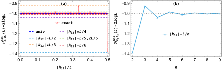
Figure 2: The Shannon entropy of the total system in the double-particle state $|k_{1}k_{2}\rangle$ of the free bosonic chain. Left: The red empty diamonds connected with thin lines are the exact bosonic result (2.18) with $L=840$. The dark blue dashed line is the result (2.19), i.e. the universal (univ) formula (2.20), which is valid for $|k_{12}|\ll L$. The other dashed lines are the exceptional result (2.21) which is valid for exceptional values of the momentum difference $|k_{12}|=\frac{mL}{n}\leq\frac{L}{2}$ with coprime integers $m,n$. Right: The large $n$ limit of exceptional bosonic result (2.21) leads to the universal result (2.20).

2.4.2 Subsystem Shannon entropy

For the subsystem $A$, there are $\frac{(\ell+1)(\ell+2)}{2}$ possible local states and the probabilities are shown in Table 5, where we have

$$p_{0}=(1-x)^{2}+\frac{\sin^{2}(\pi k_{12}x)}{L^{2}\sin^{2}\frac{\pi k_{12}}{L}},$$ (2.23)

$$p_{j}=\frac{2(1-x)}{L}-\frac{2\sin(\pi k_{12}x)\cos\frac{2\pi k_{12}(j-\frac{\ell+1}{2})}{L}}{L^{2}\sin\frac{\pi k_{12}}{L}}.$$ (2.24)

For general $L$, $\ell$, and $k_{12}$, we get the exact subsystem Shannon entropy

$$H^{\textrm{bos}}_{k_{1}k_{2}}(\ell)=-\Big{[}(1-x)^{2}+\frac{\sin^{2}(\pi k_{12}x)}{L^{2}\sin^{2}\frac{\pi k_{12}}{L}}\Big{]}\log\Big{[}(1-x)^{2}+\frac{\sin^{2}(\pi k_{12}x)}{L^{2}\sin^{2}\frac{\pi k_{12}}{L}}\Big{]}$$

$$-\sum_{j=1}^{\ell}\Big{[}\frac{2(1-x)}{L}-\frac{2\sin(\pi k_{12}x)\cos\frac{2\pi k_{12}(j-\frac{\ell+1}{2})}{L}}{L^{2}\sin\frac{\pi k_{12}}{L}}\Big{]}\log\Big{[}\frac{2(1-x)}{L}-\frac{2\sin(\pi k_{12}x)\cos\frac{2\pi k_{12}(j-\frac{\ell+1}{2})}{L}}{L^{2}\sin\frac{\pi k_{12}}{L}}\Big{]}$$

$$+\frac{2x}{L}(2\log L-\log 2)-\sum_{j=1}^{\ell-1}(\ell-j)\frac{4}{L^{2}}\cos^{2}\frac{\pi jk_{12}}{L}\log\Big{(}\frac{4}{L^{2}}\cos^{2}\frac{\pi jk_{12}}{L}\Big{)}.$$ (2.25)

For $|k_{12}|\ll L$ in the scaling limit $L\to+\infty$, $\ell\to+\infty$ with fixed $x={\ell}/{L}$, we get the Shannon entropy

$$H^{\textrm{bos}}_{k_{1}k_{2}}(\ell)=2x\log L-2x\log 2-\Big{[}(1-x)^{2}+\frac{\sin^{2}(\pi k_{12}x)}{\pi^{2}k_{12}^{2}}\Big{]}\log\Big{[}(1-x)^{2}+\frac{\sin^{2}(\pi k_{12}x)}{\pi^{2}k_{12}^{2}}\Big{]}$$

$$\phantom{H^{\textrm{bos}}_{k_{1}k_{2}}(\ell)=}-4\int_{0}^{x/2}\!\!\mathrm{d}y\Big{[}(1-x)-\frac{\sin(\pi k_{12}x)\cos(2\pi k_{12}y)}{\pi k_{12}}\Big{]}\log\Big{[}(1-x)-\frac{\sin(\pi k_{12}x)\cos(2\pi k_{12}y)}{\pi k_{12}}\Big{]}$$

$$\phantom{H^{\textrm{bos}}_{k_{1}k_{2}}(\ell)=}-4\int_{0}^{k_{12}x}\!\!\frac{\mathrm{d}z}{k_{12}}\Big{(}x-\frac{z}{k_{12}}\Big{)}\cos^{2}(\pi z)\log\cos^{2}(\pi z).$$ (2.26)

For $1\ll|k_{12}|\ll L$ in the scaling limit, we get the universal result

$$H^{\textrm{univ}}_{k_{1}k_{2}}(\ell)=2x\log L-2(1-x)\log(1-x)-x^{2}-2x(1-x)\log 2,$$ (2.27)

which is the same as neither the result for two identical classical particles $H^{\textrm{cl}}_{1^{2}}(\ell)$ (A.23) nor the result for two distinguishable classical particles $H^{\textrm{cl}}_{12}(\ell)$ (A.26). As we will see in the subsequent section, the universal result also applies to the double-particle state $|k_{1}k_{2}\rangle$ in the free fermionic theory.

local states	probabilities	ranges	numbers
$|G\rangle_{A}$	$p_{0}$ (2.23)	-	1
$|j\rangle_{A}$	$p_{j}$ (2.24)	$j\in[1,\ell]$	$\ell$
$|j^{2}\rangle_{A}$	$p_{j^{2}}=\frac{2}{L^{2}}$	$j\in[1,\ell]$	$\ell$
$|j_{1}j_{2}\rangle_{A}$	$p_{j_{1}j_{2}}=\frac{4}{L^{2}}\cos^{2}\frac{\pi j_{12}k_{12}}{L}$	$1\leq j_{1}<j_{2}\leq\ell$	$\frac{\ell(\ell-1)}{2}$

Table 5: The local states and probabilities of the subsystem $A$ in the double-particle state $|k_{1}k_{2}\rangle$ of the free bosonic chain.

For exceptional values of the momentum difference $|k_{12}|=\frac{mL}{n}\leq\frac{L}{2}$ with coprime integers $m,n$ in the scaling limit $L\to+\infty$, $\ell\to+\infty$ with fixed $x={\ell}/{L}$, we get exceptional value of the subsystem Shannon entropy

$$\mathcal{H}^{\textrm{bos}}_{k_{1}k_{2}}(\ell)=2x\log L-2x\log 2-2(1-x)\log(1-x)-\frac{2x^{2}}{n}\sum_{a=1}^{n-1}\cos^{2}\frac{\pi a}{n}\log\cos^{2}\frac{\pi a}{n}.$$ (2.28)

Note that the $x\to 1$ limit of (2.28) is just (2.21) as it should be. Also, the $n\to+\infty$ limit of the exceptional result (2.28) leads to the universal result (2.27).

In summary, we have obtained four formulas for the subsystem Shannon entropy, i.e. the exact formula (2.4.2) which is valid for general $L$, $\ell$, and $k_{12}$, the formula (2.4.2) which is valid for $|k_{12}|\ll L$ in the scaling limit $L\to+\infty$, $\ell\to+\infty$ with fixed $x={\ell}/{L}$, the universal formula (2.27) which is valid for $1\ll|k_{12}|\ll L$ in the scaling limit, the exceptional formula (2.28) which is valid for the exceptional values $|k_{12}|=\frac{mL}{n}\leq\frac{L}{2}$ with coprime integers $m,n$ in the scaling limit. We show these results in Figure 3, where in the left panel we see the large $|k_{12}|$ limit of the bosonic result (2.4.2), which gives the universal result (2.27), and in the right panel we see the large $n$ limit of the exceptional result (2.28), which also gives the universal result (2.27).

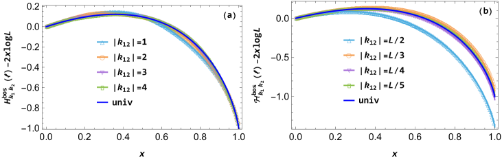
Figure 3: The subsystem Shannon entropy in the double-particle state $|k_{1}k_{2}\rangle$ of the free bosonic chain. The empty symbols are the exact result (2.4.2) with $L=240$. The dark blue solid lines are the universal result (2.27) which is valid for $1\ll|k_{12}|\ll L$. In the left panel the other solid lines are the result (2.4.2) which is valid for $|k_{12}|\ll L$, and in the right panel the other solid lines are the exceptional result (2.28) which is valid for exceptional values $|k_{12}|=\frac{mL}{n}\leq\frac{L}{2}$ with coprime integers $m,n$.

2.4.3 Subsystem Shannon mutual information

Using the results of the total system and subsystem Shannon entropies in different parameter regimes, we evaluate the subsystem Shannon mutual information. From (2.18) and (2.4.2), we obtain the exact mutual information $M^{\textrm{bos}}_{k_{1}k_{2}}(\ell)$ that is valid for general $L$, $\ell$, $k_{12}$. From (2.19) and (2.4.2), we obtain the mutual information

$$M^{\textrm{bos}}_{k_{1}k_{2}}(\ell)=H^{\textrm{bos}}_{k_{1}k_{2}}(\ell)+H^{\textrm{bos}}_{k_{1}k_{2}}(L-\ell)-H^{\textrm{bos}}_{k_{1}k_{2}}(L),$$ (2.29)

which is valid for $|k_{12}|\ll L$ in the scaling limit. From (2.19) and (2.27), we further obtain the universal mutual information

$$M^{\textrm{univ}}_{k_{1}k_{2}}(\ell)=-2x\log{x}-2(1-x)\log{(1-x)}-2x(1-x)(2\log{2}-1),$$ (2.30)

which is valid for $1\ll|k_{12}|\ll L$ in the scaling limit. From (2.21) and (2.28), we obtain the exceptional mutual information

$$\mathcal{M}^{\textrm{bos}}_{k_{1}k_{2}}(\ell)=-2x\log{x}-2(1-x)\log{(1-x)}+\frac{4x(1-x)}{n}\sum_{a=1}^{n-1}\cos^{2}\frac{\pi a}{n}\log\cos^{2}\frac{\pi a}{n},$$ (2.31)

which is valid for the exceptional values $|k_{12}|=\frac{mL}{n}\leq\frac{L}{2}$ with coprime integers $m,n$. In the scaling limit, the Shannon mutual information is a finite function of the ratio $x={\ell}/{L}$. Surprisingly, both the results (2.30) and (2.31) are generally different from the result for two distinguishable classical particles $M^{\textrm{cl}}_{12}(\ell)$ (A.27). Only for the special case with $|k_{12}|=\frac{L}{2}$, there is $\mathcal{M}^{\textrm{bos}}_{k_{1}k_{2}}(\ell)=M^{\textrm{cl}}_{12}(\ell)$. The results (2.30) and (2.31) are also different from the result for two identical classical particles $M^{\textrm{cl}}_{1^{2}}(\ell)$ (A.24). We show the subsystem Shannon mutual information in Figure 4.

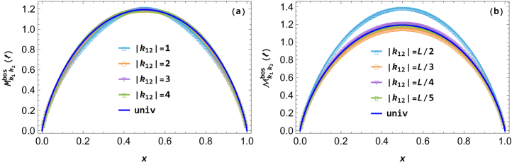
Figure 4: The subsystem Shannon mutual information in the double-particle state $|k_{1}k_{2}\rangle$ of the free bosonic chain. The empty symbols are the exact result with $L=240$. The dark blue solid lines are the universal result (2.30) which is valid for $1\ll|k_{12}|\ll L$. In the left panel the other solid lines are the result which is valid for $|k_{12}|\ll L$, and in the right panel the other solid lines are the exceptional result (2.31) which is valid for the exceptional values $|k_{12}|=\frac{mL}{n}\leq\frac{L}{2}$ with coprime integers $m,n$.

3 Free fermionic chain

This section deals with the single-particle state $|k\rangle$ and double-particle state $|k_{1}k_{2}\rangle$ in the free fermionic chain. The case of the free fermionic chain resembles that of the free bosonic chain, so we will keep it brief in this section.

3.1 Quasiparticle excited states

The free fermionic chain has the Hamiltonian

$$H=\sum_{j=1}^{L}\Big{(}a_{j}^{\dagger}a_{j}-\frac{1}{2}\Big{)}.$$ (3.1)

We define the global modes

$$b_{k}^{\dagger}\equiv\frac{1}{\sqrt{L}}\sum_{j=1}^{L}\mathrm{e}^{\frac{2\pi\mathrm{i}jk}{L}}a_{j}^{\dagger},~{}b_{k}\equiv\frac{1}{\sqrt{L}}\sum_{j=1}^{L}\mathrm{e}^{-\frac{2\pi\mathrm{i}jk}{L}}a_{j},~{}k=1,2,\cdots,L.$$ (3.2)

The ground state is defined as

$$a_{j}|G\rangle=b_{k}|G\rangle=0,~{}\forall j,\forall k.$$ (3.3)

Using the global modes $b_{k}^{\dagger}$, one could construct the general global state

$$|k_{1}k_{2}\cdots k_{s}\rangle=b_{k_{1}}^{\dagger}b_{k_{2}}^{\dagger}\cdots b_{k_{s}}^{\dagger}|G\rangle.$$ (3.4)

Like the free bosonic chain, the natural local basis at each site is the eigenstates of the excitation number operator. One could also use the modes $a_{j}^{\dagger}$ to construct the general locally excited state

$$|j_{1}j_{2}\cdots j_{s}\rangle=a_{j_{1}}^{\dagger}a_{j_{2}}^{\dagger}\cdots a_{j_{s}}^{\dagger}|G\rangle.$$ (3.5)

In the Hilbert space of the subsystem $A=[1,\ell]$, one has similarly the subsystem ground state $|G\rangle_{A}$ defined as

$$a_{j}|G\rangle_{A}=0,~{}\forall j\in A,$$ (3.6)

as well as the subsystem local states

$$|j_{1}j_{2}\cdots j_{s}\rangle_{A}=a_{j_{1}}^{\dagger}a_{j_{2}}^{\dagger}\cdots a_{j_{s}}^{\dagger}|G\rangle_{A},~{}j_{1},j_{2},\cdots,j_{s}\in A.$$ (3.7)

3.2 Single-particle state $|k\rangle$

We can use the same calculations and results as for the single particle state $|k\rangle$ in the free bosonic chain in subsection 2.2. We will skip them here.

3.3 Double-particle state $|k_{1}k_{2}\rangle$

This subsection deals with the calculation of Shannon entropy in the double-particle state $|k_{1}k_{2}\rangle=b^{\dagger}_{k_{1}}b^{\dagger}_{k_{2}}|G\rangle$ in free fermionic chain.

3.3.1 Total system Shannon entropy

We write the double-particle state $|k_{1}k_{2}\rangle$ in terms of local states as

$$|k_{1}k_{2}\rangle=\frac{2\mathrm{i}}{L}\sum_{1\leq j_{1}<j_{2}\leq L}e^{\frac{\pi\mathrm{i}}{L}(j_{1}+j_{2})(k_{1}+k_{2})}\sin\frac{\pi j_{12}k_{12}}{L}|j_{1}j_{2}\rangle,$$ (3.8)

with $j_{12}=j_{1}-j_{2}$ and $k_{12}=k_{1}-k_{2}$.

There are $\frac{L(L-1)}{2}$ possible local states $|j_{1}j_{2}\rangle$ with $1\leq j_{1}<j_{2}\leq L$, and the corresponding probabilities are

$$p_{j_{1}j_{2}}=\frac{4}{L^{2}}\sin^{2}\frac{\pi j_{12}k_{12}}{L},~{}1\leq j_{1}<j_{2}\leq L.$$ (3.9)

For general $L$ and $k_{12}$, we get the Shannon entropy of the total system

$$H^{\textrm{fer}}_{k_{1}k_{2}}(L)=2\log L-2\log 2-\frac{4}{L}\sum_{j=1}^{L/2-1}\sin^{2}\frac{\pi jk_{12}}{L}\log\sin^{2}\frac{\pi jk_{12}}{L}.$$ (3.10)

For $|k_{12}|\ll L$ in the limit $L\to+\infty$, the Shannon entropy becomes

$$H^{\textrm{fer}}_{k_{1}k_{2}}(L)=2\log L-1,$$ (3.11)

which is the same as the bosonic result $H^{\textrm{bos}}_{k_{1}k_{2}}(L)$ (2.19) and the universal result $H^{\textrm{univ}}_{k_{1}k_{2}}(L)$ (2.20).

For the exceptional value $|k_{12}|=\frac{mL}{n}\leq\frac{L}{2}$ with coprime integers $m,n$, we get the exceptional Shannon entropy

$$\mathcal{H}^{\textrm{fer}}_{k_{1}k_{2}}(L)=2\log L-2\log 2-\frac{2}{n}\sum_{a=1}^{n-1}\sin^{2}\frac{\pi a}{n}\log\sin^{2}\frac{\pi a}{n}.$$ (3.12)

Explicitly, for $n=\{2,3,4,5,6\}$, we get respectively

$$\mathcal{H}^{\textrm{fer}}_{k_{1}k_{2}}(L)-2\log L=\Big{\{}-2\log 2,-\log 3,-\frac{3}{2}\log 2,$$

$$\phantom{\mathcal{H}^{\textrm{fer}}_{k_{1}k_{2}}(L)-2\log L=}\log 2-\frac{1}{10}[(5-\sqrt{5})\log(5-\sqrt{5})+(5+\sqrt{5})\log(5+\sqrt{5})],$$

$$\phantom{\mathcal{H}^{\textrm{fer}}_{k_{1}k_{2}}(L)-2\log L=}-\frac{2}{3}\log 2-\frac{1}{2}\log 3\Big{\}},$$ (3.13)

which are generally different from the exceptional bosonic results (2.4.1).

We show these various results in Figure 5.

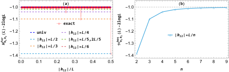
Figure 5: The Shannon entropy of the total system in the double-particle state $|k_{1}k_{2}\rangle$ of the free fermionic chain. Left: The red empty diamonds connected with thin lines are the exact result (3.10) with $L=840$. The dark blue dashed line is the result (3.11), i.e. the universal formula (2.20), which is valid for $|k_{12}|\ll L$. The other dashed lines are the exceptional result (3.12) which is valid for exceptional values of the momentum difference $|k_{12}|=\frac{mL}{n}\leq\frac{L}{2}$ with coprime integers $m,n$. Right: The large $n$ limit of the exceptional result (3.12) leads to the universal result (2.20).

3.3.2 Subsystem Shannon entropy

For the subsystem $A$, there are $\frac{\ell(\ell+1)}{2}+1$ possible local states and the probabilities are shown in Table 6, where we have

$$p_{0}=(1-x)^{2}-\frac{\sin^{2}(\pi k_{12}x)}{L^{2}\sin^{2}\frac{\pi k_{12}}{L}},$$ (3.14)

$$p_{j}=\frac{2(1-x)}{L}+\frac{2\sin(\pi k_{12}x)\cos\frac{2\pi k_{12}(j-\frac{\ell+1}{2})}{L}}{L^{2}\sin\frac{\pi k_{12}}{L}}.$$ (3.15)

For general $L$, $\ell$, and $k_{12}$, we get the exact subsystem Shannon entropy

$$H^{\textrm{fer}}_{k_{1}k_{2}}(\ell)=-\Big{[}(1-x)^{2}-\frac{\sin^{2}(\pi k_{12}x)}{L^{2}\sin^{2}\frac{\pi k_{12}}{L}}\Big{]}\log\Big{[}(1-x)^{2}-\frac{\sin^{2}(\pi k_{12}x)}{L^{2}\sin^{2}\frac{\pi k_{12}}{L}}\Big{]}$$

$$-\sum_{j=1}^{\ell}\Big{[}\frac{2(1-x)}{L}+\frac{2\sin(\pi k_{12}x)\cos\frac{2\pi k_{12}(j-\frac{\ell+1}{2})}{L}}{L^{2}\sin\frac{\pi k_{12}}{L}}\Big{]}\log\Big{[}\frac{2(1-x)}{L}+\frac{2\sin(\pi k_{12}x)\cos\frac{2\pi k_{12}(j-\frac{\ell+1}{2})}{L}}{L^{2}\sin\frac{\pi k_{12}}{L}}\Big{]}$$

$$-\sum_{j=1}^{\ell-1}(\ell-j)\frac{4}{L^{2}}\sin^{2}\frac{\pi jk_{12}}{L}\log\Big{(}\frac{4}{L^{2}}\sin^{2}\frac{\pi jk_{12}}{L}\Big{)}.$$ (3.16)

For $|k_{12}|\ll L$ in the scaling limit $L\to+\infty$, $\ell\to+\infty$ with fixed $x={\ell}/{L}$, we get the Shannon entropy

$$H^{\textrm{fer}}_{k_{1}k_{2}}(\ell)=2x\log L-2x\log 2-\Big{[}(1-x)^{2}-\frac{\sin^{2}(\pi k_{12}x)}{\pi^{2}k_{12}^{2}}\Big{]}\log\Big{[}(1-x)^{2}-\frac{\sin^{2}(\pi k_{12}x)}{\pi^{2}k_{12}^{2}}\Big{]}$$

$$\phantom{H^{\textrm{fer}}_{k_{1}k_{2}}(\ell)=}-4\int_{0}^{x/2}\!\!\mathrm{d}y\Big{[}(1-x)+\frac{\sin(\pi k_{12}x)\cos(2\pi k_{12}y)}{\pi k_{12}}\Big{]}\log\Big{[}(1-x)+\frac{\sin(\pi k_{12}x)\cos(2\pi k_{12}y)}{\pi k_{12}}\Big{]}$$

$$\phantom{H^{\textrm{fer}}_{k_{1}k_{2}}(\ell)=}-4\int_{0}^{k_{12}x}\!\!\frac{\mathrm{d}z}{k_{12}}\Big{(}x-\frac{z}{k_{12}}\Big{)}\sin^{2}(\pi z)\log\sin^{2}(\pi z).$$ (3.17)

For $1\ll k_{12}\ll L$ in the scaling limit, we get the universal result $H^{\textrm{univ}}_{k_{1}k_{2}}(\ell)$ (2.27).

local states	probabilities	ranges	numbers
$|G\rangle_{A}$	$p_{0}$ (3.14)	-	1
$|j\rangle_{A}$	$p_{j}$ (3.15)	$j\in[1,\ell]$	$\ell$
$|j_{1}j_{2}\rangle_{A}$	$p_{j_{1}j_{2}}=\frac{4}{L^{2}}\sin^{2}\frac{\pi j_{12}k_{12}}{L}$	$1\leq j_{1}<j_{2}\leq\ell$	$\frac{\ell(\ell-1)}{2}$

Table 6: The local states and probabilities of the subsystem $A$ in the double-particle state $|k_{1}k_{2}\rangle$ of the free fermionic chain.

For exceptional values of the momentum difference $|k_{12}|=\frac{mL}{n}\leq\frac{L}{2}$ with coprime integers $m,n$ in the scaling limit $L\to+\infty$, $\ell\to+\infty$ with fixed $x={\ell}/{L}$, we get the subsystem Shannon entropy

$$\mathcal{H}^{\textrm{fer}}_{k_{1}k_{2}}(\ell)=2x\log L-2x\log 2-2(1-x)\log(1-x)-\frac{2x^{2}}{n}\sum_{a=1}^{n-1}\sin^{2}\frac{\pi a}{n}\log\sin^{2}\frac{\pi a}{n}.$$ (3.18)

We show the various results in Figure 6.

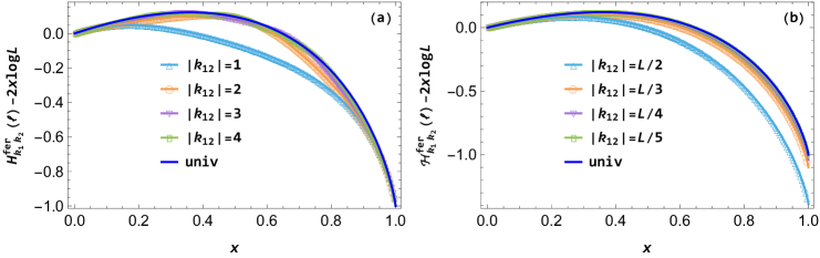
Figure 6: The subsystem Shannon entropy in the double-particle state $|k_{1}k_{2}\rangle$ of the free fermionic chain. The empty symbols are the exact result (3.3.2) with $L=240$. The dark blue solid lines are the universal result (2.27) which is valid for $1\ll|k_{12}|\ll L$. In the left panel the other solid lines are the result (3.3.2) which is valid for $|k_{12}|\ll L$, and in the right panel the other solid lines are the exceptional result (3.18) which is valid for the exceptional values $|k_{12}|=\frac{mL}{n}\leq\frac{L}{2}$ with coprime integers $m,n$.

3.3.3 Subsystem Shannon mutual information

With the results of the total system and subsystem Shannon entropies in different regimes of the parameters, we calculate the subsystem Shannon mutual information. From (3.10) and (3.3.2), we obtain the exact fermionic mutual information $M^{\textrm{fer}}_{k_{1}k_{2}}(\ell)$ that is valid for general $L$, $\ell$, $k_{12}$. From (3.11) and (3.3.2), we obtain

$$M^{\textrm{fer}}_{k_{1}k_{2}}(\ell)=H^{\textrm{fer}}_{k_{1}k_{2}}(\ell)+H^{\textrm{fer}}_{k_{1}k_{2}}(L-\ell)-H^{\textrm{fer}}_{k_{1}k_{2}}(L),$$ (3.19)

which is valid for $|k_{12}|\ll L$ in the scaling limit. From (3.11) and (2.27), we obtain the universal mutual information $M^{\textrm{univ}}_{k_{1}k_{2}}(\ell)$ which is the same as (2.30) and is valid for $1\ll|k_{12}|\ll L$ in the scaling limit. From (3.12) and (3.18), we obtain the exceptional mutual information

$$\mathcal{M}^{\textrm{fer}}_{k_{1}k_{2}}(\ell)=-2x\log{x}-2(1-x)\log{(1-x)}+\frac{4x(1-x)}{n}\sum_{a=1}^{n-1}\sin^{2}\frac{\pi a}{n}\log\sin^{2}\frac{\pi a}{n},$$ (3.20)

which is valid for the exceptional values of the momentum difference $|k_{12}|=\frac{mL}{n}\leq\frac{L}{2}$ with coprime integers $m,n$. We show the subsystem mutual information in Figure 7.

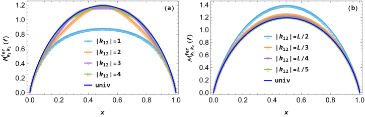
Figure 7: The subsystem Shannon mutual information in the double-particle state $|k_{1}k_{2}\rangle$ of the free fermionic chain. The empty symbols are the exact result with $L=240$. The dark blue solid lines are the universal result (2.30) which is valid for $1\ll|k_{12}|\ll L$. In the left panel the other solid lines are the result (3.19) which is valid for $|k_{12}|\ll L$, and in the right panel the other solid lines are the exceptional result (3.20) which is valid for the exceptional values $|k_{12}|=\frac{mL}{n}\leq\frac{L}{2}$ with coprime integers $m,n$.

4 XXX chain

In this section, we compute the Shannon entropy of the total system and its subsystem and the subsystem mutual information in single- and double-magnon excited states of the spin-1/2 XXX chain. The single-magnon state results are identical to those for the single-particle states in free bosonic and fermionic chains. The double-magnon state is more complex, as it can be either a scattering state or a bound state. The total system Shannon entropy part in this section has overlaps with [9].

4.1 Magnon excited states

We consider the spin-1/2 XXX chain

$$H=-\frac{1}{4}\sum_{j=1}^{L}(\sigma_{j}^{x}\sigma_{j+1}^{x}+\sigma_{j}^{y}\sigma_{j+1}^{y}+\sigma_{j}^{z}\sigma_{j+1}^{z})-\frac{h}{2}\sum_{j=1}^{L}\sigma_{j}^{z},$$ (4.1)

with a positive transverse field $h>0$ and periodic boundary conditions for the Pauli matrices $\sigma_{L+1}^{x,y,z}=\sigma_{1}^{x,y,z}$. For simplicity, we also require that the number of sites $L$ is four times of an integer. The unique ground state is

$$|G\rangle=|\!\uparrow\uparrow\cdots\uparrow\rangle.$$ (4.2)

The low-lying eigenstates are magnon excited states in the ferromagnetic phase and can be obtained from the coordinate Bethe ansatz [55, 56]. One may use the Bethe numbers of the excited magnons $\{I_{1},I_{2},\cdots,I_{s}\}$ to denote magnon excited states as $|I_{1}I_{2}\cdots I_{s}\rangle$.

Unlike for the free bosonic and fermionic chains, there is no natural local basis at each site for the XXX chain. We choose the eigenstates of $\sigma_{j}^{z}$ as the local basis at each site in this paper. There are also local states, such as

$$|j\rangle=|\!\cdots\downarrow_{j}\cdots\rangle,$$ (4.3)

in which only the site $j$ has downward spin and all other sites have upward spins, and

$$|j_{1}j_{2}\rangle=|\!\cdots\downarrow_{j_{1}}\cdots\downarrow_{j_{2}}\cdots\rangle,$$ (4.4)

in which only the sites $j_{1},j_{2}$ have downward spins and all other sites have upward spins. For the subsystem $A$, there are the subsystem local states $|G\rangle_{A}$ in which all the sites in $A$ has upward spins, $|j\rangle_{A}$ in which only the site $j$ in $A$ has downward spin, and $|j_{1}j_{2}\rangle_{A}$ in which only the sites $j_{1},j_{2}$ in $A$ have downward spins.

4.2 Single-magnon state

The single magnon state takes the form

$$|I\rangle=\frac{1}{\sqrt{L}}\sum_{j=1}^{L}\mathrm{e}^{\frac{2\pi\mathrm{i}jI}{L}}|j\rangle,$$ (4.5)

with the Bethe number $I=0,1,\cdots,L-1$. The total system Shannon entropy and the subsystem Shannon entropy and mutual information are the same as those of one-particle states in the free bosonic and fermionic chains in, respectively, subsections 2.2 and 3.2 and the configurations of one soft-core and hard-core classical particles in, respectively, subsections A.1.1 and A.2.1. We will not repeat the calculations here.

4.3 Double-magnon state

We consider the double-magnon state

$$|I_{1}I_{2}\rangle=\frac{1}{\sqrt{\mathcal{N}}}\sum_{1\leq j_{1}<j_{2}\leq L}\mathcal{U}_{j_{1}j_{2}}|j_{1}j_{2}\rangle,$$ (4.6)

with the Bethe numbers $I_{1},I_{2}$ which are integers and satisfy $0\leq I_{1}\leq I_{2}\leq L-1$. There is

$$\mathcal{U}_{j_{1}j_{2}}=\mathrm{e}^{\mathrm{i}(j_{1}p_{1}+j_{2}p_{2}+\frac{\theta}{2})}+\mathrm{e}^{\mathrm{i}(j_{1}p_{2}+j_{2}p_{1}-\frac{\theta}{2})},$$ (4.7)

with $p_{1},p_{2},\theta$ being solutions to the equation

$$\mathrm{e}^{\mathrm{i}\theta}=-\frac{1+\mathrm{e}^{\mathrm{i}(p_{1}+p_{2})}-2\mathrm{e}^{\mathrm{i}p_{1}}}{1+\mathrm{e}^{\mathrm{i}(p_{1}+p_{2})}-2\mathrm{e}^{\mathrm{i}p_{2}}}.$$ (4.8)

The normalization factor is

$$\mathcal{N}=\sum_{1\leq j_{1}<j_{2}\leq L}|\mathcal{U}_{j_{1}j_{2}}|^{2}.$$ (4.9)

In the state $|I_{1}I_{2}\rangle$ there are two magnons with physical momenta $p_{1},p_{2}$ and momenta $k_{1},k_{2}$ related as

$$p_{1}=\frac{2\pi k_{1}}{L},~{}p_{2}=\frac{2\pi k_{2}}{L}.$$ (4.10)

To the equation (4.8), there are three cases of solutions, namely case I solution, case II solutions, and case III solutions. The case III solutions could be further classified into case IIIa solutions and case IIIb solutions.

4.3.1 Case I solution

For the case I solution, there are trivially

$$I_{1}=p_{1}=k_{1}=I_{2}=p_{2}=k_{2}=\theta=0,$$ (4.11)

and the state is

$$|00\rangle=\sqrt{\frac{2}{L(L-1)}}\sum_{1\leq j_{1}<j_{2}\leq L}|j_{1}j_{2}\rangle.$$ (4.12)

The probability of the local state $|j_{1}j_{2}\rangle$ is

$$p^{\textrm{I}}_{j_{1}j_{2}}=\frac{2}{L(L-1)},~{}1\leq j_{1}<j_{2}\leq L,$$ (4.13)

which is the same as the probability distribution (A.11) in the configuration of two identical hard-core classical particles in subsection A.2.2. The total system Shannon entropy $H^{{\textrm{I}}}_{00}(L)$ and subsystem Shannon entropy $H^{{\textrm{I}}}_{00}(\ell)$ and mutual information $M^{{\textrm{I}}}_{00}(\ell)$ in state $|00\rangle$ are, respectively, the same as $H^{\textrm{hard}}_{1^{2}}(L)$ (A.12), $H^{\textrm{hard}}_{1^{2}}(\ell)$ (A.13), and $M^{\textrm{hard}}_{1^{2}}(\ell)$ (A.2.2). We will not repeat the calculations here.

4.3.2 Case II solution

For one case II solution $|I_{1}I_{2}\rangle$, there are

$$k_{1}=I_{1}+\frac{\theta}{2\pi},~{}k_{2}=I_{2}-\frac{\theta}{2\pi},$$ (4.14)

with Bethe numbers $I_{1},I_{2}$ which satisfy $0\leq I_{1}<I_{2}\leq L-1$ and real shift angle $\theta\in[0,\pi]$. We have

$$k_{12}=I_{12}+\frac{\theta}{\pi},$$ (4.15)

with the momentum difference $k_{12}=k_{1}-k_{2}$ and Bethe number difference $I_{12}=I_{1}-I_{2}$. The normalization factor is

$$\mathcal{N}=L(L-1)+\frac{L\cos(\theta-p_{12})-(L-1)\cos\theta-\cos(\theta-Lp_{12})}{1-\cos p_{12}}.$$ (4.16)

The probability that one finds the total system in the local state $|j_{1}j_{2}\rangle$ is

$$p^{\textrm{II}}_{j_{1}j_{2}}=\frac{2}{\mathcal{N}}[1+\cos(j_{12}p_{12}+\theta)],~{}1\leq j_{1}<j_{2}\leq L,$$ (4.17)

with $j_{12}=j_{1}-j_{2}$ and $p_{12}=p_{1}-p_{2}$. For the subsystem $A$, the probabilities of the subsystem local states $|G\rangle_{A}$, $|j\rangle_{A}$, and $|j_{1}j_{2}\rangle_{A}$ are, respectively,

$$p^{\textrm{II}}_{0}=\frac{1}{\mathcal{N}}\Big{[}(L-\ell)(L-\ell-1)+\frac{(L-\ell)\cos(p_{12}-\theta)-(L-\ell-1)\cos\theta-\cos[(L-\ell)p_{12}-\theta]}{1-\cos p_{12}}\Big{]},$$ (4.18)

$$p^{\textrm{II}}_{j}=\frac{2}{\mathcal{N}}\Big{[}L-\ell+\frac{\sin\frac{p_{12}(L-\ell)}{2}\cos[p_{12}(j-\frac{L+\ell+1}{2})+\theta]}{\sin\frac{p_{12}}{2}}\Big{]},~{}j\in[1,\ell],$$ (4.19)

$$p^{\textrm{II}}_{j_{1}j_{2}}=\frac{2}{\mathcal{N}}[1+\cos(j_{12}p_{12}+\theta)],~{}1\leq j_{1}<j_{2}\leq\ell.$$ (4.20)

From these probabilities, we obtain for general parameters $L$, $\ell$, $I_{1}$ and $I_{2}$ the total system Shannon entropy and the subsystem Shannon entropy and mutual information

$$H^{\textrm{II}}_{I_{1}I_{2}}(L)=-\sum_{1\leq j_{1}<j_{2}\leq L}p^{\textrm{II}}_{j_{1}j_{2}}\log p^{\textrm{II}}_{j_{1}j_{2}},$$ (4.21)

$$H^{\textrm{II}}_{I_{1}I_{2}}(\ell)=-p^{\textrm{II}}_{0}\log p^{\textrm{II}}_{0}-\sum_{j=1}^{\ell}p^{\textrm{II}}_{j}\log p^{\textrm{II}}_{j}-\sum_{1\leq j_{1}<j_{2}\leq\ell}p^{\textrm{II}}_{j_{1}j_{2}}\log p^{\textrm{II}}_{j_{1}j_{2}},$$ (4.22)

$$M^{\textrm{II}}_{I_{1}I_{2}}(\ell)=H^{\textrm{II}}_{I_{1}I_{2}}(\ell)+H^{\textrm{II}}_{I_{1}I_{2}}(L-\ell)-H^{\textrm{II}}_{I_{1}I_{2}}(L).$$ (4.23)

We are interested in how the above results (4.21), (4.22) and (4.23) behave in the scaling limit $L\to+\infty$, $\ell\to+\infty$ with fixed ratio $x={\ell}/{L}$. We define the scaled Bethe numbers

$$\iota_{1}=\lim_{L\to+\infty}\frac{I_{1}}{L},~{}\iota_{2}=\lim_{L\to+\infty}\frac{I_{2}}{L}.$$ (4.24)

When $\iota_{1}=\iota_{2}=0$ or $\iota_{1}=\iota_{2}=1$ or $\iota_{1}=0,\iota_{2}=1$, we have $\theta\to 0$ and obtain

$$\lim_{L\to+\infty}H^{\textrm{II}}_{I_{1}I_{2}}(L)=H^{\textrm{bos}}_{k_{1}k_{2}}(L),~{}\lim_{L\to+\infty}H^{\textrm{II}}_{I_{1}I_{2}}(\ell)=H^{\textrm{bos}}_{k_{1}k_{2}}(\ell),$$

$$\lim_{L\to+\infty}M^{\textrm{II}}_{I_{1}I_{2}}(\ell)=M^{\textrm{bos}}_{k_{1}k_{2}}(\ell),~{}k_{12}=I_{12},$$ (4.25)

with $H^{\textrm{bos}}_{k_{1}k_{2}}(L)$ (2.19), $H^{\textrm{bos}}_{k_{1}k_{2}}(\ell)$ (2.4.2) and $M^{\textrm{bos}}_{k_{1}k_{2}}(\ell)$ (2.29) being the bosonic results in the scaling limit. When $\iota_{1}=\iota_{2}\in(0,1)$, we have $\theta\to\pi$ and the results approach to the fermionic results

$$\lim_{L\to+\infty}H^{\textrm{II}}_{I_{1}I_{2}}(L)=H^{\textrm{fer}}_{k_{1}k_{2}}(L),~{}\lim_{L\to+\infty}H^{\textrm{II}}_{I_{1}I_{2}}(\ell)=H^{\textrm{fer}}_{k_{1}k_{2}}(\ell),$$

$$\lim_{L\to+\infty}M^{\textrm{II}}_{I_{1}I_{2}}(\ell)=M^{\textrm{fer}}_{k_{1}k_{2}}(\ell),~{}k_{12}=I_{12}+1,$$ (4.26)

with $H^{\textrm{fer}}_{k_{1}k_{2}}(L)$ (3.11), $H^{\textrm{fer}}_{k_{1}k_{2}}(\ell)$ (3.3.2) and $M^{\textrm{fer}}_{k_{1}k_{2}}(\ell)$ (3.19). When $0\leq\iota_{1}<\iota_{2}\leq 1$, excluding the case $\iota_{1}=0,\iota_{2}=1$, we have $\theta\in[0,\pi)$ and the results approach to the universal results

$$\lim_{L\to+\infty}H^{\textrm{II}}_{I_{1}I_{2}}(L)=H^{\textrm{univ}}_{k_{1}k_{2}}(L),~{}\lim_{L\to+\infty}H^{\textrm{II}}_{I_{1}I_{2}}(\ell)=H^{\textrm{univ}}_{k_{1}k_{2}}(\ell),~{}\lim_{L\to+\infty}M^{\textrm{II}}_{I_{1}I_{2}}(\ell)=M^{\textrm{univ}}_{k_{1}k_{2}}(\ell),$$ (4.27)

with $H^{\textrm{univ}}_{k_{1}k_{2}}(L)$ (2.20), $H^{\textrm{univ}}_{k_{1}k_{2}}(\ell)$ (2.27) and $M^{\textrm{univ}}_{k_{1}k_{2}}(\ell)$ (2.30). Note that the universal results do not depend on the actual values of the momenta $k_{1},k_{2}$. The exact numerical results of the total system Shannon entropy, subsystem Shannon entropy and mutual information, and the corresponding analytical results in the scaling limit are shown in Figure 8.

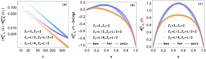
Figure 8: The total system Shannon entropy (left), subsystem Shannon entropy (middle) and mutual information (right) in the case II double-magnon state $|I_{1}I_{2}\rangle$ of the XXX chain. The empty symbols are the exact numerical results. In the middle and right panels we have set $L=240$ for the exact results, and the solid lines are the corresponding analytical results in the scaling limit, namely the bosonic (bos) results $H^{\textrm{bos}}_{k_{1}k_{2}}(\ell)$ (2.4.2) and $M^{\textrm{bos}}_{k_{1}k_{2}}(\ell)$ (2.29) with $|k_{12}|=1$, fermionic (fer) results $H^{\textrm{fer}}_{k_{1}k_{2}}(\ell)$ (3.3.2) and $M^{\textrm{fer}}_{k_{1}k_{2}}(\ell)$ (3.19) with $|k_{12}|=1$, and the universal results $H^{\textrm{univ}}_{k_{1}k_{2}}(\ell)$ (2.27) and $M^{\textrm{univ}}_{k_{1}k_{2}}(\ell)$ (2.30).

4.3.3 Case IIIa solution

For a case IIIa solution, there are Bethe numbers

$$I_{1}=\frac{I-1}{2},~{}I_{2}=\frac{I+1}{2},$$ (4.28)

with the total Bethe number

$$I=\tilde{I},\tilde{I}+2,\cdots,\frac{L}{2}-1,\frac{3L}{2}+1,\frac{3L}{2}+3,\cdots,2L-\tilde{I},$$ (4.29)

where $\tilde{I}$ is an odd integer around $2\sqrt{L}/\pi$ in $L\to+\infty$ limit. Without loss of generality, we only need to consider $I=\tilde{I},\tilde{I}+2,\cdots,\frac{L}{2}-1$. The solution to the Bethe equation is

$$p_{1}=\frac{\pi I}{L}+\mathrm{i}v,~{}p_{2}=\frac{\pi I}{L}-\mathrm{i}v,~{}\theta=\pi+\mathrm{i}Lv.$$ (4.30)

In $L\to+\infty$ limit, there is

$$v=-\log\Big{|}\cos\frac{\pi I}{L}\Big{|},$$ (4.31)

which is in the range

$$\frac{2}{L}\lesssim v\lesssim\log\frac{L}{\pi}.$$ (4.32)

One could understand $1/v$ as the size of the bound state. The normalization factor is

$$\mathcal{N}=L\Big{[}\frac{\sinh[(L-1)v]}{\sinh v}-(L-1)\Big{]}.$$ (4.33)

The probability that one finds the total system in the local state $|j_{1}j_{2}\rangle$ is

$$p^{\textrm{IIIa}}_{j_{1}j_{2}}=\frac{4}{\mathcal{N}}\sinh^{2}\Big{[}v\Big{(}j_{12}+\frac{L}{2}\Big{)}\Big{]},~{}1\leq j_{1}<j_{2}\leq L,$$ (4.34)

with $j_{12}=j_{1}-j_{2}$. For the subsystem $A$, the probabilities of the subsystem local states $|G\rangle_{A}$, $|j\rangle_{A}$, and $|j_{1}j_{2}\rangle_{A}$ are, respectively,

$$p^{\textrm{IIIa}}_{0}=\frac{1}{\mathcal{N}}\Big{[}(L-\ell)\frac{\sinh[v(L-1)]}{\sinh v}-\frac{\sinh(v\ell)\sinh[v(L-\ell)]}{\sinh^{2}v}-(L-\ell)(L-\ell-1)\Big{]},$$ (4.35)

$$p^{\textrm{IIIa}}_{j}=\frac{2}{\mathcal{N}}\Big{[}\frac{\sinh[v(L-\ell)]\cosh[2v(j-\frac{\ell+1}{2})]}{\sinh v}-(L-\ell)\Big{]},~{}j\in[1,\ell],$$ (4.36)

$$p^{\textrm{IIIa}}_{j_{1}j_{2}}=\frac{4}{\mathcal{N}}\sinh^{2}\Big{[}v\Big{(}j_{12}+\frac{L}{2}\Big{)}\Big{]},~{}1\leq j_{1}<j_{2}\leq\ell.$$ (4.37)

From these probabilities, we obtain for general parameters $L$, $\ell$, and $I$ the total system Shannon entropy and the subsystem Shannon entropy and mutual information

$$H^{\textrm{IIIa}}_{I_{1}I_{2}}(L)=-\sum_{1\leq j_{1}<j_{2}\leq L}p^{\textrm{IIIa}}_{j_{1}j_{2}}\log p^{\textrm{IIIa}}_{j_{1}j_{2}},$$ (4.38)

$$H^{\textrm{IIIa}}_{I_{1}I_{2}}(\ell)=-p^{\textrm{IIIa}}_{0}\log p^{\textrm{IIIa}}_{0}-\sum_{j=1}^{\ell}p^{\textrm{IIIa}}_{j}\log p^{\textrm{IIIa}}_{j}-\sum_{1\leq j_{1}<j_{2}\leq\ell}p^{\textrm{IIIa}}_{j_{1}j_{2}}\log p^{\textrm{IIIa}}_{j_{1}j_{2}},$$ (4.39)

$$M^{\textrm{IIIa}}_{I_{1}I_{2}}(\ell)=H^{\textrm{IIIa}}_{I_{1}I_{2}}(\ell)+H^{\textrm{IIIa}}_{I_{1}I_{2}}(L-\ell)-H^{\textrm{IIIa}}_{I_{1}I_{2}}(L).$$ (4.40)

For finite $v$, we have in the limit $L\to+\infty$

$$p^{\textrm{IIIa}}_{j_{1}j_{2}}\to\frac{2\sinh v}{L}\mathrm{e}^{2v(|j_{12}+\frac{L}{2}|-\frac{L-1}{2})},~{}1\leq j_{1}<j_{2}\leq L,$$ (4.41)

and in the scaling limit there are

$$p^{\textrm{IIIa}}_{0}\to 1-x,$$ (4.42)

$$p^{\textrm{IIIa}}_{j}\to\frac{1}{L}\mathrm{e}^{-2v(\frac{\ell-1}{2}-|j-\frac{\ell+1}{2}|)},~{}j\in[1,\ell],$$ (4.43)

$$p^{\textrm{IIIa}}_{j_{1}j_{2}}\to\frac{2\sinh v}{L}\mathrm{e}^{-2v(\frac{L-1}{2}-|j_{12}+\frac{L}{2}|)},~{}1\leq j_{1}<j_{2}\leq\ell.$$ (4.44)

We obtain the tightly bound limit of the Shannon entropies and mutual information

$$H^{\textrm{IIIa}}_{I_{1}I_{2}}(L)=\log L-\log(2\sinh v)+v\coth v,$$ (4.45)

$$H^{\textrm{IIIa}}_{I_{1}I_{2}}(\ell)=x[\log L-\log(2\sinh v)+v\coth v]-(1-x)\log(1-x),$$ (4.46)

$$M^{\textrm{IIIa}}_{I_{1}I_{2}}(\ell)=-x\log x-(1-x)\log(1-x).$$ (4.47)

Note that the total system Shannon entropy (4.45) has been obtained in [9]. Although the bound state has finite width $1/v$, the mutual information (4.47) does not depend on $v$. Further $v\to+\infty$ limit leads to the single-particle results

$$H^{\textrm{IIIa}}_{I_{1}I_{2}}(L)=\log L,$$ (4.48)

$$H^{\textrm{IIIa}}_{I_{1}I_{2}}(\ell)=x\log L-(1-x)\log(1-x),$$ (4.49)

$$M^{\textrm{IIIa}}_{I_{1}I_{2}}(\ell)=-x\log x-(1-x)\log(1-x).$$ (4.50)

For $v=\frac{u}{L}$ with finite $u$, which leads to

$$u=-\lim_{L\to+\infty}L\log\Big{|}\cos\frac{\pi I}{L}\Big{|},$$ (4.51)

we get the loosely bound limit of the results

$$H^{\textrm{IIIa}}_{I_{1}I_{2}}(L)=2\log L+\log\Big{(}\frac{\sinh u}{u}-1\Big{)}-2\log 2-\frac{4}{\frac{\sinh u}{u}-1}\int_{0}^{\frac{u}{2}}\!\frac{\mathrm{d}y}{u}\sinh^{2}y\log\sinh^{2}y,$$ (4.52)

$$H^{\textrm{IIIa}}_{I_{1}I_{2}}(\ell)=2x\log L+\Big{(}x+\frac{\frac{\sinh(ux)\sinh[u(1-x)]}{u^{2}}-x(1-x)}{\frac{\sinh u}{u}-1}\Big{)}\log\Big{(}\frac{\sinh u}{u}-1\Big{)}-2x\log 2$$

$$\phantom{H^{\textrm{IIIa}}_{I_{1}I_{2}}(L)=}-\Big{(}1-x-\frac{\frac{\sinh(ux)\sinh[u(1-x)]}{u^{2}}-x(1-x)}{\frac{\sinh u}{u}-1}\Big{)}\log\Big{(}1-x-\frac{\frac{\sinh(ux)\sinh[u(1-x)]}{u^{2}}-x(1-x)}{\frac{\sinh u}{u}-1}\Big{)}$$

$$\phantom{H^{\textrm{IIIa}}_{I_{1}I_{2}}(L)=}-\frac{4}{\frac{\sinh u}{u}-1}\int_{0}^{\frac{x}{2}}\!\mathrm{d}y\Big{[}\frac{\sinh[u(1-x)]\cosh(2uy)}{u}-(1-x)\Big{]}\log\Big{[}\frac{\sinh[u(1-x)]\cosh(2uy)}{u}-(1-x)\Big{]}$$

$$\phantom{H^{\textrm{IIIa}}_{I_{1}I_{2}}(L)=}-\frac{4}{\frac{\sinh u}{u}-1}\int_{0}^{x}\!\mathrm{d}y(x-y)\sinh^{2}\Big{[}u\Big{(}y-\frac{1}{2}\Big{)}\Big{]}\log\sinh^{2}\Big{[}u\Big{(}y-\frac{1}{2}\Big{)}\Big{]},$$ (4.53)

$$M^{\textrm{IIIa}}_{I_{1}I_{2}}(\ell)=H^{\textrm{IIIa}}_{I_{1}I_{2}}(\ell)+H^{\textrm{IIIa}}_{I_{1}I_{2}}(L-\ell)-H^{\textrm{IIIa}}_{I_{1}I_{2}}(L).$$ (4.54)

We show the total system Shannon entropy, subsystem Shannon entropy and mutual information in the case IIIa double-magnon state $|I_{1}I_{2}\rangle$ of the XXX chain, as well as their tightly bound and loosely bound limits, in Figure 9. We see that in the range $I/L\in(0,0.5)$ the results of the loosely bound limit apply for relatively small $I/L\gtrsim 0$ while the results of the tightly bound limit apply for relatively large $I/L\lesssim 0.5$. For the total system and subsystem Shannon entropies, there is the range $0.1\lesssim I/L\lesssim 0.3$ in which both the results of the loosely bound limit and the results of the tightly bound limit apply.

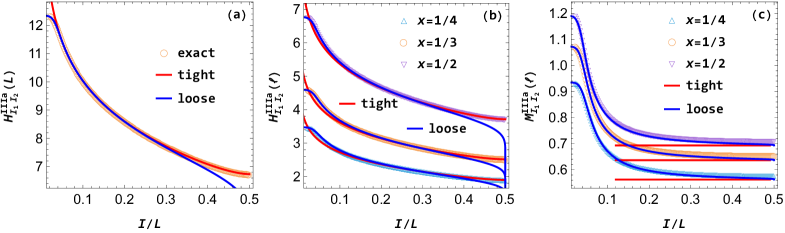
Figure 9: The total system Shannon entropy (left), subsystem Shannon entropy (middle) and mutual information (right) in the case IIIa double-magnon state $|I_{1}I_{2}\rangle$ of the XXX chain. The empty symbols are the exact numerical results. The solid red and blue lines are, respectively, results of the tightly bound limit (4.45), (4.46) and (4.47), and results of the loosely bound limit (4.52), (4.53) and (4.54). We have set $L=840$.

4.3.4 Case IIIb solution

For a case IIIb solution, there are Bethe numbers

$$I_{1}=I_{2}=\frac{I}{2},$$ (4.55)

with the total Bethe number

$$I=2,4,\cdots,\frac{L}{2},\frac{3L}{2},\frac{3L}{2}+2,\cdots,2L-2.$$ (4.56)

In the case with $I=\frac{L}{2}$, the state is extremely bound

$$|I_{1}I_{2}\rangle=\frac{1}{\sqrt{L}}\sum_{j=1}^{L}\mathrm{e}^{\frac{2\pi\mathrm{i}I}{L}(j+\frac{1}{2})}|j,j+1\rangle,$$ (4.57)

the results are the same as the those in the single-magnon state in subsection 4.2, and we will not repeat the calculations in this paper. Without loss of generality, we only consider $I=2,4,\cdots,\frac{L}{2}-2$. The solution to the equation (4.8) is

$$p_{1}=\frac{\pi I}{L}+\mathrm{i}v,~{}p_{2}=\frac{\pi I}{L}-\mathrm{i}v,~{}\theta=\mathrm{i}Lv.$$ (4.58)

In $L\to+\infty$ limit, there is still

$$v=-\log\Big{|}\cos\frac{\pi I}{L}\Big{|},$$ (4.59)

which is in the range

$$\frac{2\pi^{2}}{L^{2}}\lesssim v\lesssim\log\frac{L}{\pi}.$$ (4.60)

The normalization factor is

$$\mathcal{N}=L\Big{[}\frac{\sinh[(L-1)v]}{\sinh v}+(L-1)\Big{]}.$$ (4.61)

The probability that one finds the total system in the local state $|j_{1}j_{2}\rangle$ is

$$p^{\textrm{IIIb}}_{j_{1}j_{2}}=\frac{4}{\mathcal{N}}\cosh^{2}\Big{[}v\Big{(}j_{12}+\frac{L}{2}\Big{)}\Big{]},~{}1\leq j_{1}<j_{2}\leq L,$$ (4.62)

with $j_{12}=j_{1}-j_{2}$. For the subsystem $A$, the probabilities of the subsystem local states $|G\rangle_{A}$, $|j\rangle_{A}$, and $|j_{1}j_{2}\rangle_{A}$ are, respectively,

$$p^{\textrm{IIIb}}_{0}=\frac{1}{\mathcal{N}}\Big{[}(L-\ell)\frac{\sinh[v(L-1)]}{\sinh v}-\frac{\sinh(v\ell)\sinh[v(L-\ell)]}{\sinh^{2}v}+(L-\ell)(L-\ell-1)\Big{]},$$ (4.63)

$$p^{\textrm{IIIb}}_{j}=\frac{2}{\mathcal{N}}\Big{[}\frac{\sinh[v(L-\ell)]\cosh[2v(j-\frac{\ell+1}{2})]}{\sinh v}+(L-\ell)\Big{]},~{}j\in[1,\ell],$$ (4.64)

$$p^{\textrm{IIIb}}_{j_{1}j_{2}}=\frac{4}{\mathcal{N}}\cosh^{2}\Big{[}v\Big{(}j_{12}+\frac{L}{2}\Big{)}\Big{]},~{}1\leq j_{1}<j_{2}\leq\ell.$$ (4.65)

We obtain for general parameters $L$, $\ell$, and $I$ the total system Shannon entropy and the subsystem Shannon entropy and mutual information

$$H^{\textrm{IIIb}}_{I_{1}I_{2}}(L)=-\sum_{1\leq j_{1}<j_{2}\leq L}p^{\textrm{IIIb}}_{j_{1}j_{2}}\log p^{\textrm{IIIb}}_{j_{1}j_{2}},$$ (4.66)

$$H^{\textrm{IIIb}}_{I_{1}I_{2}}(\ell)=-p^{\textrm{IIIb}}_{0}\log p^{\textrm{IIIb}}_{0}-\sum_{j=1}^{\ell}p^{\textrm{IIIb}}_{j}\log p^{\textrm{IIIb}}_{j}-\sum_{1\leq j_{1}<j_{2}\leq\ell}p^{\textrm{IIIb}}_{j_{1}j_{2}}\log p^{\textrm{IIIb}}_{j_{1}j_{2}},$$ (4.67)

$$M^{\textrm{IIIb}}_{I_{1}I_{2}}(\ell)=H^{\textrm{IIIb}}_{I_{1}I_{2}}(\ell)+H^{\textrm{IIIb}}_{I_{1}I_{2}}(L-\ell)-H^{\textrm{IIIb}}_{I_{1}I_{2}}(L).$$ (4.68)

For finite $v$, we obtain the same tightly bound results as those in case IIIa states

$$H^{\textrm{IIIb}}_{I_{1}I_{2}}(L)=\log L-\log(2\sinh v)+v\coth v,$$ (4.69)

$$H^{\textrm{IIIb}}_{I_{1}I_{2}}(\ell)=x[\log L-\log(2\sinh v)+v\coth v]-(1-x)\log(1-x),$$ (4.70)

$$M^{\textrm{IIIb}}_{I_{1}I_{2}}(\ell)=-x\log x-(1-x)\log(1-x).$$ (4.71)

Further $v\to+\infty$ limit leads to the single-particle results

$$H^{\textrm{IIIb}}_{I_{1}I_{2}}(L)=\log L,$$ (4.72)

$$H^{\textrm{IIIb}}_{I_{1}I_{2}}(\ell)=x\log L-(1-x)\log(1-x),$$ (4.73)

$$M^{\textrm{IIIb}}_{I_{1}I_{2}}(\ell)=-x\log x-(1-x)\log(1-x).$$ (4.74)

For $v=\frac{u}{L}$ with fixed $u$ in the scaling limit, we get the loosely bound limit of the results

$$H^{\textrm{IIIb}}_{I_{1}I_{2}}(L)=2\log L+\log\Big{(}\frac{\sinh u}{u}+1\Big{)}-2\log 2-\frac{4}{\frac{\sinh u}{u}+1}\int_{0}^{\frac{u}{2}}\!\frac{\mathrm{d}y}{u}\cosh^{2}y\log\cosh^{2}y,$$ (4.75)

$$H^{\textrm{IIIb}}_{I_{1}I_{2}}(\ell)=2x\log L+\Big{(}x+\frac{\frac{\sinh(ux)\sinh[u(1-x)]}{u^{2}}+x(1-x)}{\frac{\sinh u}{u}+1}\Big{)}\log\Big{(}\frac{\sinh u}{u}+1\Big{)}-2x\log 2$$

$$\phantom{H^{\textrm{IIIb}}_{I_{1}I_{2}}(L)=}-\Big{(}1-x-\frac{\frac{\sinh(ux)\sinh[u(1-x)]}{u^{2}}+x(1-x)}{\frac{\sinh u}{u}+1}\Big{)}\log\Big{(}1-x-\frac{\frac{\sinh(ux)\sinh[u(1-x)]}{u^{2}}+x(1-x)}{\frac{\sinh u}{u}+1}\Big{)}$$

$$\phantom{H^{\textrm{IIIb}}_{I_{1}I_{2}}(L)=}-\frac{4}{\frac{\sinh u}{u}+1}\int_{0}^{\frac{x}{2}}\!\mathrm{d}y\Big{[}\frac{\sinh[u(1-x)]\cosh(2uy)}{u}+(1-x)\Big{]}\log\Big{[}\frac{\sinh[u(1-x)]\cosh(2uy)}{u}+(1-x)\Big{]}$$

$$\phantom{H^{\textrm{IIIb}}_{I_{1}I_{2}}(L)=}-\frac{4}{\frac{\sinh u}{u}+1}\int_{0}^{x}\!\mathrm{d}y(x-y)\cosh^{2}\Big{[}u\Big{(}y-\frac{1}{2}\Big{)}\Big{]}\log\cosh^{2}\Big{[}u\Big{(}y-\frac{1}{2}\Big{)}\Big{]},$$ (4.76)

$$M^{\textrm{IIIb}}_{I_{1}I_{2}}(\ell)=H^{\textrm{IIIb}}_{I_{1}I_{2}}(\ell)+H^{\textrm{IIIb}}_{I_{1}I_{2}}(L-\ell)-H^{\textrm{IIIb}}_{I_{1}I_{2}}(L).$$ (4.77)

A further $u\to 0$ limit of (4.75), (4.76), and (4.77) leads to

$$H^{\textrm{IIIb}}_{I_{1}I_{2}}(L)=2\log L-\log 2,$$ (4.78)

$$H^{\textrm{IIIb}}_{I_{1}I_{2}}(\ell)=2x\log L-2(1-x)\log(1-x)-x(2-x)\log 2,$$ (4.79)

$$M^{\textrm{IIIb}}_{I_{1}I_{2}}(\ell)=-x^{2}\log x^{2}-2x(1-x)\log[2x(1-x)]-(1-x)^{2}\log(1-x)^{2},$$ (4.80)

which are the same as the results of two identical classical particles $H^{\textrm{cl}}_{1^{2}}(L)$ (A.22), $H^{\textrm{cl}}_{1^{2}}(\ell)$ (A.23), and $M^{\textrm{cl}}_{1^{2}}(\ell)$ (A.24). For $v=\frac{w}{L^{2}}$ with fixed $w$ in the scaling limit, we get the same results (4.78), (4.79), and (4.80).

We show the total system Shannon entropy, subsystem Shannon entropy and mutual information in the case IIIb double-magnon state $|I_{1}I_{2}\rangle$ of the XXX chain, as well as their tightly and loosely bound limits, in Figure 10.

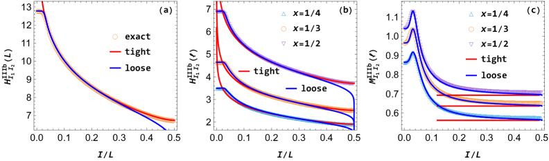
Figure 10: The total system Shannon entropy (left), subsystem Shannon entropy (middle) and mutual information (right) in the case IIIb double-magnon state $|I_{1}I_{2}\rangle$ of the XXX chain. The empty symbols are the exact numerical results. The solid red and blue lines are, respectively, the tightly bound results (4.69), (4.70) and (4.71), and the loosely bound results (4.75), (4.76) and (4.77). We have set $L=840$.

5 Conclusion and discussion

In this paper we have presented an analysis of the total system Shannon entropy, subsystem Shannon entropy, and subsystem Shannon mutual information in quasiparticle excited states of free bosonic and fermionic chains, as well as the XXX chain. We compared the results across different spin chains and contrasted them with those of classical particles. Our findings indicate that, like the entanglement entropy, the formulas for the Shannon entropy in free bosonic and fermionic chains also apply to the Shannon entropy in the XXX chain, subject to certain limits. Additionally, we found that even when two quasiparticles have a large momentum difference, their contributions to the Shannon entropy do not decouple, unlike the entanglement entropy. Furthermore, we discovered universal formulas for the total system Shannon entropy, subsystem Shannon entropy, and mutual information in the limit of large momentum differences, which are valid for free bosonic and fermionic chains, as well as the XXX chain, but differ from any results obtained from classical particles. In other words, we did not observe any semiclassical quasiparticle picture that could reproduce the universal results of the Shannon entropy in quantum spin chains.

The existence of universal formulas in various quantum chains that differ from any classical results is a puzzle. It has been found that the semiclassical quasiparticle picture explains the existence of universal entanglement entropy in quantum chains [41, 42]. However, no such explanation exists for the local basis Shannon entropy. In the main text of the paper, we have calculated the Shannon entropy using a particular basis of local states. However, it is essential to note that the definition of the Shannon entropy is dependent on the chosen basis. If one selects the eigenstates of the density matrix as the basis, the Shannon entropy will become equivalent to the von Neumann entropy for both pure and mixed quantum states of the total system or its subsystem. For quantum spin chains, the eigenstates of the subsystem particle number operator are also a natural basis. In Appendix B, we have studied the Shannon entropy of the subsystem particle number probability distribution in free bosonic and fermionic chains. We have found that the semiclassical quasiparticle picture applies in the large momentum difference limit. In Appendix C, we have calculated the Shannon entropy in the local basis of the $\sigma_{j}^{x}$ eigenstates in the XXX chain. The results are significantly different from those obtained using the $\sigma_{j}^{z}$ basis. Even in the single-magnon state, the $\sigma_{j}^{x}$ basis Shannon entropy is already nontrivial. In certain limits, there exist forms of universal results for which no semiclassical quasiparticle picture applies.

In summary, we have found Shannon entropy in local bases for which no semiclassical quasiparticle picture applies. At the same time, there are the entanglement entropy, subsystem distance and Shannon entropy of the subsystem particle number probability distribution for which the semiclassical quasiparticle picture applies in the large momentum difference limit. We anticipate that the semiclassical picture applies to course-grained properties but not to fine-grained properties. In other words, if one scrutinizes the microscopic details of a quasiparticle excited state, one can distinguish between quasiparticles and real particles. However, for a measure of certain macroscopic properties, quasiparticles behave similarly to real particles.

In this paper, our primary focus has been on one- and double-particle states. However, we believe that exploring states with multiple quasiparticles would be a worthwhile endeavor. We anticipate that the properties described in our study will still hold true for such states.

Experimental realization of excited states in spin chains was demonstrated in trapped atomic ion systems [57, 58, 59]. Recently, a proposal has been put forward to utilize neutral atom arrays to simulate fermionic many-body systems [60]. It would be fascinating to measure the Shannon entropy in quasiparticle excited states of spin chains and compare the experimental outcomes with the results presented in this paper. For example, by measuring the subsystem Shannon entropy in a double-particle state with a small momentum difference, one could tell whether the excitations are bosonic or fermionic.

Appendix A Classical particles

This appendix presents the calculation of the Shannon entropy and mutual information for classical particle configurations on a circular chain. Both soft-core and hard-core particles are considered, corresponding to the classical limits of bosonic and fermionic quantum particles, respectively.

A.1 Soft-core classical particles

We start with soft-core classical particles, which can have any number of particles at one site, i.e. a site can be empty, occupied by one particle, or occupied by more than one particle.

A.1.1 One particle

We consider the macroscopic configuration of the chain in which there is one soft-core classical particle. There are $L$ possible microscopic configurations, i.e. the particle at site $j$ with $j\in[1,L]$, and probabilities are

$$p_{j}=\frac{1}{L},~{}j\in[1,L].$$ (A.1)

The Shannon entropy of the whole system is

$$H^{\textrm{soft}}_{1}(L)=\log{L}.$$ (A.2)

For the subsystem $A$, there are $\ell+1$ possible microscopic configurations, as shown in Table 7. The Shannon entropy of the subsystem $A$ is

$$H^{\textrm{soft}}_{1}(\ell)=x\log L-(1-x)\log(1-x).$$ (A.3)

The Shannon mutual information is

$$M^{\textrm{soft}}_{1}(\ell)=-x\log x-(1-x)\log(1-x),$$ (A.4)

which is just the Shannon entropy of the probability distribution of the coarse-grained subsystem configurations $\{x,1-x\}$. Observe that the values of $1-x$ and $x$ correspond to the presence of no particle and one particle, respectively, in the subsystem $A$.

microscopic configurations	probabilities	ranges	numbers
no particle in $A$	$p_{0}=1-x$	-	1
one particle in $A$ at $j$	$p_{j}=\frac{1}{L}$	$j\in[1,\ell]$	$\ell$

Table 7: The microscopic configurations and probabilities of the subsystem $A$ in the macroscopic configuration of one soft-core classical particle.

A.1.2 Two identical particles

We consider the macroscopic configuration in which there are two identical particles on the chain. For the total system, there are $\frac{L(L+1)}{2}$ possible microscopic configurations as shown in Table 8. In the scaling limit, the Shannon entropy of the total system is

$$H^{\textrm{soft}}_{1^{2}}(L)=2\log L-\log 2.$$ (A.5)

microscopic configurations	probabilities	ranges	numbers
both at $j$	$p_{j^{2}}=\frac{1}{L^{2}}$	$j\in[1,L]$	$L$
one at $j_{1}$ and the other at $j_{2}$	$p_{j_{1}j_{2}}=\frac{2}{L^{2}}$	$1\leq j_{1}<j_{2}\leq L$	$\frac{L(L-1)}{2}$

Table 8: The microscopic configurations and probabilities of the total system in the macroscopic configuration of two identical soft-core classical particles.

For the subsystem $A$, there are $\frac{(\ell+1)(\ell+2)}{2}$ different microscopic configurations, as shown in Table 9. In the scaling limit, we get the Shannon entropy of the subsystem $A$

$$H^{\textrm{soft}}_{1^{2}}(\ell)=2x\log L-x(2-x)\log 2-2(1-x)\log(1-x).$$ (A.6)

In the scaling limit, the mutual information is

$$M^{\textrm{soft}}_{1^{2}}(\ell)=-x^{2}\log x^{2}-2x(1-x)\log[2x(1-x)]-(1-x)^{2}\log(1-x)^{2}$$

$$\phantom{M^{\textrm{soft}}_{1^{2}}(\ell)}=-2x\log x-2(1-x)\log(1-x)-2x(1-x)\log 2,$$ (A.7)

which is just the Shannon entropy of the probability distribution of the coarse-grained subsystem configurations $\{x^{2},2x(1-x),(1-x)^{2}\}$.

microscopic configurations	probabilities	ranges	numbers
no particle in $A$	$p_{0}=(1-x)^{2}$	-	1
only one particle in $A$ at $j$	$p_{j}=\frac{2(1-x)}{L}$	$j\in[1,\ell]$	$\ell$
both in $A$ at $j$	$p_{j^{2}}=\frac{1}{L^{2}}$	$j\in[1,\ell]$	$\ell$
both in $A$ with one at $j_{1}$ and the other at $j_{2}$	$p_{j_{1}j_{2}}=\frac{2}{L^{2}}$	$1\leq j_{1}<j_{2}\leq\ell$	$\frac{\ell(\ell-1)}{2}$

Table 9: The microscopic configurations and probabilities of the subsystem $A$ in the macroscopic configuration of two identical soft-core classical particles.

A.1.3 Two distinguishable particle

We consider two distinguishable particles, say one red particle and one blue particle. There are $L^{2}$ possible microscopic configurations, as shown in Table 10. The Shannon entropy is

$$H^{\textrm{soft}}_{12}(L)=2\log L.$$ (A.8)

microscopic configurations	probabilities	ranges	numbers
both at $j$	$p_{j^{2}}=\frac{1}{L^{2}}$	$j\in[1,L]$	$L$
red at $j_{1}$ with blue at $j_{2}$	$p_{j_{1}j_{2}}=\frac{1}{L^{2}}$	$j_{1},j_{2}\in[1,L]$, $j_{1}\neq j_{2}$	$L(L-1)$

Table 10: The microscopic configurations and probabilities of the total system in the macroscopic configuration of two distinguishable soft-core classical particles.

For the subsystem $A$, there are $(\ell+1)(\ell+2)$ possible configurations, as shown in Table 11. We get the Shannon entropy of the subsystem

$$H^{\textrm{soft}}_{12}(\ell)=2x\log L-2(1-x)\log(1-x).$$ (A.9)

The mutual information is

$$M^{\textrm{soft}}_{12}(\ell)=2[-x\log x-(1-x)\log(1-x)],$$ (A.10)

which is just the Shannon entropy of the probability distribution of the coarse-grained subsystem configurations $\{x,1-x\}\otimes\{x,1-x\}=\{x^{2},x(1-x),x(1-x),(1-x)^{2}\}$.

microscopic configurations	probabilities	ranges	numbers
no particle in $A$	$p_{0}=(1-x)^{2}$	-	1
only red particle in $A$ at $j$	$p_{j}^{\rm red}=\frac{1-x}{L}$	$j\in[1,\ell]$	$\ell$
only blue particle in $A$ at $j$	$p_{j}^{\rm blue}=\frac{1-x}{L}$	$j\in[1,\ell]$	$\ell$
both in $A$ at $j$	$p_{j^{2}}=\frac{1}{L^{2}}$	$j=1,2,\cdots,L$	$\ell$
both in $A$ with red at $j_{1}$ and blue at $j_{2}$	$p_{j_{1}j_{2}}=\frac{1}{L^{2}}$	$j_{1},j_{2}\in[1,\ell]$, $j_{1}\neq j_{2}$	${\ell(\ell-1)}$

Table 11: The microscopic configurations and probabilities of the subsystem $A$ in the macroscopic configuration of two distinguishable soft-core classical particles.

A.2 Hard-core classical particles

We next consider classical particles with the restriction that a site can have only one particle at most.

A.2.1 One particle

This case of one hard-core classical particle is identical to that of one soft-core classical particle in subsection A.1.1. We will skip it here.

A.2.2 Two identical particles

We consider two identical hard-core classical particles. There are $\frac{L(L-1)}{2}$ possible microscopic configurations, i.e. that one particle at site $j_{1}$ and the other particle at site $j_{2}$ with $1\leq j_{1}<j_{2}\leq L$, and the corresponding probabilities are

$$p_{j_{1}j_{2}}=\frac{2}{L(L-1)},~{}1\leq j_{1}<j_{2}\leq L.$$ (A.11)

In the scaling limit, the Shannon entropy of the total system is

$$H^{\textrm{hard}}_{1^{2}}(L)=2\log L-\log 2.$$ (A.12)

For the subsystem $A$, there are $\frac{\ell(\ell+1)}{2}+1$ possible configurations, as shown in Table 12. In the scaling limit, we get the Shannon entropy of the subsystem

$$H^{\textrm{hard}}_{1^{2}}(\ell)=2x\log L-2(1-x)\log(1-x)-x(2-x)\log 2.$$ (A.13)

In the scaling limit, the mutual information is

$$M^{\textrm{hard}}_{1^{2}}(\ell)=-2x\log x-2(1-x)\log(1-x)-2x(1-x)\log 2$$

$$\phantom{M^{\textrm{hard}}_{1^{2}}(\ell)}=-x^{2}\log x^{2}-2x(1-x)\log[2x(1-x)]-(1-x)^{2}\log(1-x)^{2},$$ (A.14)

which is just the Shannon entropy of the probability distribution $\{x^{2},2x(1-x),(1-x)^{2}\}$. In the scaling limit, the results in this subsection are the same as those in subsection A.1.2.

microscopic configurations	probabilities	ranges	numbers
no particle in $A$	$p_{0}=\frac{(L-\ell)(L-\ell-1)}{L(L-1)}$	-	1
only one particle in $A$ at $j$	$p_{j}=\frac{2(L-\ell)}{L(L-1)}$	$j\in[1,\ell]$	$\ell$
both in $A$ with at $j_{1}$, $j_{2}$	$p_{j_{1}j_{2}}=\frac{2}{L(L-1)}$	$1\leq j_{1}<j_{2}\leq\ell$	$\frac{\ell(\ell-1)}{2}$

Table 12: The microscopic configurations and probabilities of the subsystem $A$ in the macroscopic configuration of two identical hard-core classical particles.

A.2.3 Two distinguishable particles

We consider two distinguishable particles, say one red particle and one blue particle. There are $L(L-1)$ possible microscopic configurations, i.e. that the red particle at site $j_{1}$ and the blue particle at site $j_{2}$ with $j_{1},j_{2}\in[1,L]$ and $j_{1}\neq j_{2}$, and the corresponding probabilities are

$$p_{j_{1}j_{2}}=\frac{1}{L(L-1)},~{}j_{1},j_{2}\in[1,L],~{}j_{1}\neq j_{2}.$$ (A.15)

In the scaling limit, the Shannon entropy is

$$H^{\textrm{hard}}_{12}(L)=2\log L.$$ (A.16)

For the subsystem $A$, there are $\ell^{2}+\ell+1$ possible configurations, as shown in Table 13. In the scaling limit, we get the Shannon entropy of the subsystem

$$H^{\textrm{hard}}_{12}(\ell)=2x\log L-2(1-x)\log(1-x).$$ (A.17)

In the scaling limit, the mutual information is

$$M^{\textrm{hard}}_{12}(\ell)=2[-x\log x-(1-x)\log(1-x)],$$ (A.18)

which is just the Shannon entropy of the probability distribution $\{x,1-x\}\otimes\{x,1-x\}=\{x^{2},x(1-x),x(1-x),(1-x)^{2}\}$. In the scaling limit, the results in this subsection are the same as those in subsection A.1.3.

microscopic configurations	probabilities	ranges	numbers
no particle in $A$	$p_{0}=\frac{(L-\ell)(L-\ell-1)}{L(L-1)}$	-	1
only red particle in $A$ at $j$	$p_{j}^{\rm red}=\frac{L-\ell}{L(L-1)}$	$j\in[1,\ell]$	$\ell$
only blue particle in $A$ at $j$	$p_{j}^{\rm blue}=\frac{L-\ell}{L(L-1)}$	$j\in[1,\ell]$	$\ell$
both in $A$ with red at $j_{1}$ and blue at $j_{2}$	$p_{j_{1}j_{2}}=\frac{1}{L(L-1)}$	$j_{1},j_{2}\in[1,\ell]$, $j_{1}\neq j_{2}$	${\ell(\ell-1)}$

Table 13: The microscopic configurations and probabilities of the subsystem $A$ in the macroscopic configuration of two distinguishable hard-core classical particles.

A.3 Summary and generalization

When the number of particles is finite, the Shannon entropy and mutual information in the scaling limit only depend on the number of particles and how distinguishable they are, not on the limit of the number of particles at each site. This means that we get the same results for soft-core and hard-core classical particles in the scaling limit. Moreover, the Shannon mutual information is equal to the Shannon entropy of the probability distribution of the coarse-grained subsystem configurations.

We summarize the results in this appendix as follows. For the macroscopic configuration of one classical particle, in the scaling limit we get the total system Shannon entropy, subsystem Shannon entropy and mutual information

$$H^{\textrm{cl}}_{1}(L)=\log{L},$$ (A.19)

$$H^{\textrm{cl}}_{1}(\ell)=x\log L-(1-x)\log(1-x),$$ (A.20)

$$M^{\textrm{cl}}_{1}(\ell)=-x\log x-(1-x)\log(1-x).$$ (A.21)

For two identical classical particles, we get

$$H^{\textrm{cl}}_{1^{2}}(L)=2\log L-\log 2,$$ (A.22)

$$H^{\textrm{cl}}_{1^{2}}(\ell)=2x\log L-2(1-x)\log(1-x)-x(2-x)\log 2,$$ (A.23)

$$M^{\textrm{cl}}_{1^{2}}(\ell)=-x^{2}\log x^{2}-2x(1-x)\log[2x(1-x)]-(1-x)^{2}\log(1-x)^{2}.$$ (A.24)

For two distinguishable classical particles, we get

$$H^{\textrm{cl}}_{12}(L)=2\log L,$$ (A.25)

$$H^{\textrm{cl}}_{12}(\ell)=2x\log L-2(1-x)\log(1-x),$$ (A.26)

$$M^{\textrm{cl}}_{12}(\ell)=-2x\log x-2(1-x)\log(1-x).$$ (A.27)

For more general cases, we just show the final results without giving any calculation details. For $r$ identical particles with finite $r$ in the scaling limit $L\to+\infty$, $\ell\to+\infty$, and fixed $x={\ell}/{L}$, we obtain

$$H^{\textrm{cl}}_{1^{r}}(L)=r\log L-\log r!,$$ (A.28)

$$H^{\textrm{cl}}_{1^{r}}(\ell)=rx\log L-\sum_{i=0}^{r}C_{r}^{i}x^{i}(1-x)^{r-i}\log[i!C_{r}^{i}(1-x)^{r-i}],$$ (A.29)

$$M^{\textrm{cl}}_{1^{r}}(\ell)=-\sum_{i=0}^{r}C_{r}^{i}x^{i}(1-x)^{r-i}\log[C_{r}^{i}x^{i}(1-x)^{r-i}],$$ (A.30)

with the binomial coefficient $C_{r}^{i}\equiv\frac{r!}{i!(r-i)!}$. For $s$ different kinds of particles with the number of the $i$-th kind of particles being $r_{i}$, $i=1,2,\cdots,s$ and total number of particles $R=\sum_{i=1}^{s}r_{i}$ being finite in the scaling limit, we get

$$H^{\textrm{cl}}_{1^{r_{1}}2^{r_{2}}\cdots s^{r_{s}}}(L)=\sum_{i=1}^{s}H^{\textrm{cl}}_{1^{r_{i}}}(L),$$ (A.31)

$$H^{\textrm{cl}}_{1^{r_{1}}2^{r_{2}}\cdots s^{r_{s}}}(\ell)=\sum_{i=1}^{s}H^{\textrm{cl}}_{1^{r_{i}}}(\ell),$$ (A.32)

$$M^{\textrm{cl}}_{1^{r_{1}}2^{r_{2}}\cdots s^{r_{s}}}(\ell)=\sum_{i=1}^{s}M^{\textrm{cl}}_{1^{r_{i}}}(\ell).$$ (A.33)

In the scaling limit, the contributions of different classical particles to the total system Shannon entropy, subsystem Shannon entropy and mutual information become independent. However, the Shannon entropy and mutual information of quantum quasiparticles do not exhibit such decoupling property even in the limit of large momentum difference, as shown in the main text of the paper.

Appendix B Shannon entropy of particle number probability distribution

In this section, we determine the Shannon entropy for the probability distribution of subsystem particle numbers in free bosonic and fermionic chains. The semiclassical quasiparticle picture applies to the Shannon entropy of particle number probability distribution in the large momentum difference limit.

B.1 Classical particles

For finite number of classical particles in the scaling limit, the subsystem Shannon entropy of particle number probability distribution only depends on the total number of particles $R$, regardless the distinguishability of these particles. The result is also not dependent on the limit of the particle number at one site. In the limit $R\ll\ell<L$, the result is just the Shannon entropy of a binomial probability distribution

$$H_{R}^{\textrm{cl}}(\ell)=-\sum_{r=0}^{R}C_{R}^{r}x^{r}(1-x)^{R-r}\log[C_{R}^{r}x^{r}(1-x)^{R-r}].$$ (B.1)

B.2 Free bosonic chain

In the single-particle state $|k\rangle$ and double-particle state $|k^{2}\rangle$ of the free bosonic chain, the results are trivial and the same as those of classical particles. We skip the calculations here.

In the double-particle state $|k_{1}k_{2}\rangle$, the probability of finding zero, one, and two particles in the subsystem $A=[1,\ell]$ are respectively

$$p^{\textrm{bos}}_{0}=(1-x)^{2}+\frac{\sin^{2}(\pi k_{12}x)}{L^{2}\sin^{2}\frac{\pi k_{12}}{L}},$$

$$p^{\textrm{bos}}_{1}=2\Big{[}x(1-x)-\frac{\sin^{2}(\pi k_{12}x)}{L^{2}\sin^{2}\frac{\pi k_{12}}{L}}\Big{]},$$

$$p^{\textrm{bos}}_{2}=x^{2}+\frac{\sin^{2}(\pi k_{12}x)}{L^{2}\sin^{2}\frac{\pi k_{12}}{L}}.$$ (B.2)

The corresponding Shannon entropy is just

$$H^{\textrm{bos}}_{k_{1}k_{2}}(\ell)=-p^{\textrm{bos}}_{0}\log p^{\textrm{bos}}_{0}-p^{\textrm{bos}}_{1}\log p^{\textrm{bos}}_{1}-p^{\textrm{bos}}_{2}\log p^{\textrm{bos}}_{2}.$$ (B.3)

In the large momentum limit $|k_{12}|\gg 1$, the result approaches that of two classical particles

$$\lim_{|k_{12}|\to+\infty}H^{\textrm{bos}}_{k_{1}k_{2}}(\ell)=H_{2}^{\textrm{cl}}(\ell).$$ (B.4)

B.3 Free fermionic chain

In the double-particle state $|k_{1}k_{2}\rangle$ of the free fermionic chain, the probability of finding zero, one, and two particles in the subsystem $A=[1,\ell]$ are respectively

$$p^{\textrm{fer}}_{0}=(1-x)^{2}-\frac{\sin^{2}(\pi k_{12}x)}{L^{2}\sin^{2}\frac{\pi k_{12}}{L}},$$

$$p^{\textrm{fer}}_{1}=2\Big{[}x(1-x)+\frac{\sin^{2}(\pi k_{12}x)}{L^{2}\sin^{2}\frac{\pi k_{12}}{L}}\Big{]},$$

$$p^{\textrm{fer}}_{2}=x^{2}-\frac{\sin^{2}(\pi k_{12}x)}{L^{2}\sin^{2}\frac{\pi k_{12}}{L}}.$$ (B.5)

The corresponding Shannon entropy is

$$H^{\textrm{fer}}_{k_{1}k_{2}}(\ell)=-p^{\textrm{fer}}_{0}\log p^{\textrm{fer}}_{0}-p^{\textrm{fer}}_{1}\log p^{\textrm{fer}}_{1}-p^{\textrm{fer}}_{2}\log p^{\textrm{fer}}_{2},$$ (B.6)

and in the large momentum limit $|k_{12}|\gg 1$ it also approaches that of two classical particles

$$\lim_{|k_{12}|\to+\infty}H^{\textrm{fer}}_{k_{1}k_{2}}(\ell)=H_{2}^{\textrm{cl}}(\ell).$$ (B.7)

Appendix C Shannon entropy in $\sigma_{j}^{x}$ basis of XXX chain

This appendix focuses on the investigation of the Shannon entropy in the local basis of eigenstates of $\sigma_{j}^{x}$ for the XXX chain.

C.1 The $\sigma_{j}^{x}$ basis

For a single set of Pauli matrices $\{\sigma^{x},\sigma^{y},\sigma^{z}\}$, the eigenstates of $\sigma^{x}$ is

$$|\pm\rangle=\frac{1}{\sqrt{2}}(|\!\uparrow\rangle\pm|\!\downarrow\rangle).$$ (C.1)

In the local basis of $\sigma_{j}^{x}$ eigenstates, there are local states which we denote as $|\mathcal{X}\rangle$ with $\mathcal{X}$ being a set of numbers in the range $[1,L]$. In the state $|\mathcal{X}\rangle$, the site $j\notin\mathcal{X}$ has spin $|+\rangle$ and the site $j\in\mathcal{X}$ has spin $|-\rangle$. For example, in this appendix we use the local states

$$|\varnothing\rangle=|++\cdots+\rangle,$$

$$|j\rangle=|\cdots-_{j}\cdots\rangle,$$

$$|j_{1}j_{2}\rangle=|\cdots-_{j_{1}}\cdots-_{j_{2}}\cdots\rangle,$$ (C.2)

where all the omitted sites have spin $|+\rangle$. For the total system with $L$ sites, there are $2^{L}$ states $\{|\mathcal{X}\rangle\}$ in $\sigma_{j}^{x}$ basis. For the subsystem $A=[1,\ell]$, there are similarly $2^{\ell}$ states $\{|\mathcal{X}\rangle_{A}\}$.

C.2 Ground state

In the ground state of the ferromagnetic XXX chain $|G\rangle=|\!\uparrow\uparrow\cdots\uparrow\rangle$, the probability of the local state $|\mathcal{X}\rangle$ is

$$p_{\mathcal{X}}^{G}=\frac{1}{2^{L}},$$ (C.3)

from which we get the Shannon entropy of the total system

$$H^{\textrm{XXX}}_{G}(L)=L\log 2.$$ (C.4)

Similarly, we get the probability of the local state $|\mathcal{X}\rangle_{A}$

$$p_{\mathcal{X}}^{A,G}=\frac{1}{2^{\ell}},$$ (C.5)

and the subsystem Shannon entropy

$$H^{\textrm{XXX}}_{G}(\ell)=\ell\log 2.$$ (C.6)

Note that the total system and subsystem Shannon entropies take the maximal values. The subsystem Shannon mutual information is trivial

$$M^{\textrm{XXX}}_{G}(\ell)=0.$$ (C.7)

C.3 Single-magnon state

In the single-magnon state

$$|I\rangle=\frac{1}{\sqrt{L}}\sum_{j=1}^{L}\mathrm{e}^{\frac{2\pi\mathrm{i}jI}{L}}|j\rangle,~{}I=0,1,\cdots,L-1,$$ (C.8)

the probability of the local state $|\mathcal{X}\rangle$ of the total system is

$$p_{\mathcal{X}}^{I}=\frac{1}{2^{L}L}\Big{|}\sum_{j=1}^{L}\mathrm{e}^{\frac{2\pi\mathrm{i}jI}{L}}m_{j,\mathcal{X}}\Big{|}^{2},$$ (C.9)

with $m_{j,\mathcal{X}}=1$ for $j\notin\mathcal{X}$ and $m_{j,\mathcal{X}}=-1$ for $j\in\mathcal{X}$. The total system Shannon entropy could be evaluated numerically as

$$H^{\textrm{XXX}}_{I}(L)=-\sum_{\mathcal{X}}p_{\mathcal{X}}^{I}\log p_{\mathcal{X}}^{I}.$$ (C.10)

Similarly, the probability of the subsystem local state $|\mathcal{X}\rangle_{A}$ is

$$p_{\mathcal{X}}^{A,I}=\frac{1}{2^{\ell}}\Big{(}1-\frac{\ell}{L}+\frac{1}{L}\Big{|}\sum_{j=1}^{\ell}\mathrm{e}^{\frac{2\pi\mathrm{i}jI}{L}}m_{j,\mathcal{X}}\Big{|}^{2}\Big{)},$$ (C.11)

from which we calculate the subsystem Shannon entropy as

$$H^{\textrm{XXX}}_{I}(\ell)=-\sum_{\mathcal{X}}p_{\mathcal{X}}^{A,I}\log p_{\mathcal{X}}^{A,I}.$$ (C.12)

The subsystem Shannon mutual information is

$$M^{\textrm{XXX}}_{I}(\ell)=H^{\textrm{XXX}}_{I}(\ell)+H^{\textrm{XXX}}_{I}(L-\ell)-H^{\textrm{XXX}}_{I}(L).$$ (C.13)

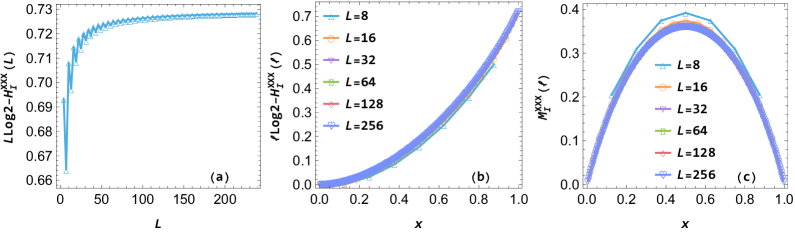
Figure 11: The $\sigma_{j}^{x}$ basis total system and subsystem Shannon entropies and mutual information in the single-magnon state of the XXX chain with Bethe numbers $I=0$ and $I=L/2$.

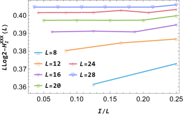
Figure 12: The $\sigma_{j}^{x}$ basis total system Shannon entropy $H^{\textrm{XXX}}_{I}(L)$ (C.10) in the single-magnon state of the XXX chain.

For the special cases $I=0$ and $I=L/2$, the formulas of the Shannon entropies $H^{\textrm{XXX}}_{I}(L)$ (C.10) and $H^{\textrm{XXX}}_{I}(\ell)$ (C.12) could be further simplified, and we obtain

$$H^{\textrm{XXX}}_{0}(L)=H^{\textrm{XXX}}_{L/2}(L)=L\log 2-\frac{1}{2^{L}}\sum_{n=0}^{L}C_{L}^{n}\Big{(}L-4n+\frac{4n^{2}}{L}\Big{)}\log\Big{(}L-4n+\frac{4n^{2}}{L}\Big{)},$$ (C.14)

$$M^{\textrm{XXX}}_{0}(L)=M^{\textrm{XXX}}_{L/2}(L)=\ell\log 2$$

$$~{}~{}~{}~{}~{}~{}~{}~{}~{}~{}~{}~{}~{}~{}~{}~{}~{}~{}~{}-\frac{1}{2^{\ell}}\sum_{n=0}^{\ell}C_{\ell}^{n}\Big{(}1+\frac{\ell^{2}-(4n+1)\ell+4n^{2}}{L}\Big{)}\log\Big{(}1+\frac{\ell^{2}-(4n+1)\ell+4n^{2}}{L}\Big{)}.$$ (C.15)

We show the special results of the total system and subsystem Shannon entropies and mutual information with $I=0$ and $I=L/2$ in Figure 11. From the left panel we see that in large $L$ limit there are

$$H^{\textrm{XXX}}_{0}(L)=H^{\textrm{XXX}}_{L/2}(L)=L\log 2-C_{0}=L\log 2-C_{L/2},$$ (C.16)

with the $L$-independent constant $C_{0}=C_{L/2}\approx 0.730$ From the middle and right panels, we see that in the scaling limit there are

$$H^{\textrm{XXX}}_{0}(\ell)=\ell\log 2-F_{0}(x)=H^{\textrm{XXX}}_{L/2}(\ell)=\ell\log 2-F_{L/2}(x),$$ (C.17)

$$M^{\textrm{XXX}}_{0}(\ell)=G_{0}(x)=M^{\textrm{XXX}}_{L/2}(\ell)=G_{L/2}(x),$$ (C.18)

with the finite functions $F_{0}(x)=F_{L/2}(x)$ and $G_{0}(x)=G_{L/2}(x)$ depending on the ratio $x={\ell}/{L}$.

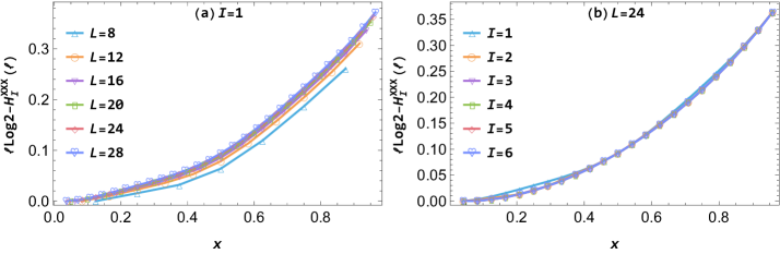
Figure 13: The $\sigma_{j}^{x}$ basis subsystem Shannon entropy $H^{\textrm{XXX}}_{I}(\ell)$ (C.12) in the single-magnon state of the XXX chain.

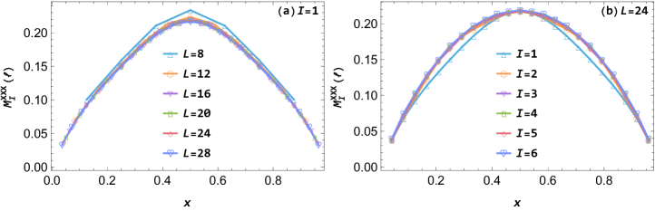
Figure 14: The $\sigma_{j}^{x}$ basis subsystem Shannon mutual information $M^{\textrm{XXX}}_{I}(\ell)$ (C.13) in the single-magnon state of the XXX chain.

For general $I$, the evaluations of the $\sigma_{j}^{x}$ basis total system Shannon entropy and the subsystem Shannon entropy and mutual information are exponentially difficult problems, and we could only numerically calculate them for not so large $L$, say $L\leq 28$. It is easy to see that both the total system and subsystem Shannon entropies $H^{\textrm{XXX}}_{I}(L)$ (C.10) and $H^{\textrm{XXX}}_{I}(\ell)$ (C.12) are invariant under the changes $I\to L-I$ and $I\to\frac{L}{2}-I$, and so without loss of generality we only need to consider $I$ in the range $[1,\frac{L}{4}]$. We show the numerical results of $H^{\textrm{XXX}}_{I}(L)$ (C.10), $H^{\textrm{XXX}}_{I}(\ell)$ (C.12), and $M^{\textrm{XXX}}_{I}(\ell)$ (C.13) in, respectively figures 12, 13 and 14. From Figure 12, we see that in large $L$ limit the total system Shannon entropy takes the form

$$H^{\textrm{XXX}}_{I}(L)=L\log 2-C_{I},$$ (C.19)

with $C_{I}$ being a constant that depends on the relative values of $I$ and $L$. We anticipate that for most values of $I$ there is the universal constant $C_{I}\approx 0.404$, and for a few exception values of $I$ the constant $C_{I}$ may take some exceptional values, like the cases $I=0$ and $I=L/2$ discussed above. From Figure 13, in the scaling limit the subsystem Shannon entropy takes the form

$$H^{\textrm{XXX}}_{I}(\ell)=\ell\log 2-F_{I}(x),$$ (C.20)

with the $I$-dependence function $F_{I}(x)$. From Figure 14, in the scaling limit the subsystem Shannon mutual information takes the form

$$M^{\textrm{XXX}}_{I}(\ell)=G_{I}(x),$$ (C.21)

with the $I$-dependence function $G_{I}(x)$. We expect that in the scaling limit, for $I\gg 1$ with a few possible exceptional values excluded, the functions $F_{I}(x)$ and $G_{I}(x)$ will take on respective universal forms.

References

- [1] M. A. Nielsen and I. L. Chuang, Quantum Computation and Quantum Information. Cambridge University Press, Cambridge, UK, 10th anniversary ed., 2010, 10.1017/CBO9780511976667.
- [2] J. Watrous, The Theory of Quantum Information. Cambridge University Press, Cambridge, UK, 2018, 10.1017/9781316848142.
- [3] M. M. Wolf, F. Verstraete, M. B. Hastings and J. I. Cirac, Area Laws in Quantum Systems: Mutual Information and Correlations, Phys. Rev. Lett. 100, 070502 (2008), [arXiv:0704.3906].
- [4] J.-M. Stéphan, S. Furukawa, G. Misguich and V. Pasquier, Shannon and entanglement entropies of one- and two-dimensional critical wave functions, Phys. Rev. B 80, 184421 (2009), [arXiv:0906.1153].
- [5] J. M. Stéphan, G. Misguich and V. Pasquier, Rényi entropy of a line in two-dimensional Ising models, Phys. Rev. B 82, 125455 (2010), [arXiv:1006.1605].
- [6] D. J. Luitz, F. Alet and N. Laflorencie, Universal Behavior beyond Multifractality in Quantum Many-Body Systems, Phys. Rev. Lett. 112, 057203 (2014), [arXiv:1308.1916].
- [7] D. J. Luitz, F. Alet and N. Laflorencie, Shannon-Rényi entropies and participation spectra across three-dimensional O (3) criticality, Phys. Rev. B 89, 165106 (2014), [arXiv:1402.4813].
- [8] D. J. Luitz, N. Laflorencie and F. Alet, Participation spectroscopy and entanglement Hamiltonian of quantum spin models, J. Stat. Mech. (2014) 08007, [arXiv:1404.3717].
- [9] Z.-Y. Dong and J.-X. Li, Confinement and oscillating deconfinement crossover of two-magnon excitations in quantum spin chains quantified by spin entanglement entropy, Phys. Rev. B 105, L220402 (2022), [arXiv:2206.08018].
- [10] H. W. Lau and P. Grassberger, Information theoretic aspects of the two-dimensional Ising model, Phys. Rev. E 87, 022128 (2013), [arXiv:1210.5707].
- [11] J.-M. Stéphan, Emptiness formation probability, Toeplitz determinants, and conformal field theory, J. Stat. Mech. (2014) 05010, [arXiv:1303.5499].
- [12] F. C. Alcaraz and M. A. Rajabpour, Universal behavior of the Shannon mutual information of critical quantum chains, Phys. Rev. Lett. 111, 017201 (2013), [arXiv:1305.1239].
- [13] J.-M. Stéphan, Shannon and Rényi mutual information in quantum critical spin chains, Phys. Rev. B 90, 045424 (2014), [arXiv:1403.6157].
- [14] F. C. Alcaraz and M. A. Rajabpour, Universal behavior of the Shannon and Rényi mutual information of quantum critical chains, Phys. Rev. B 90, 075132 (2014), [arXiv:1405.1074].
- [15] F. C. Alcaraz and M. A. Rajabpour, Generalized mutual information of quantum critical chains, Phys. Rev. B 91, 155122 (2015), [arXiv:1501.02852].
- [16] J. C. Getelina, F. C. Alcaraz and J. A. Hoyos, Entanglement properties of correlated random spin chains and similarities with conformally invariant systems, Phys. Rev. B 93, 045136 (2016), [arXiv:1511.00618].
- [17] K. Najafi and M. A. Rajabpour, Formation probabilities and Shannon information and their time evolution after quantum quench in the transverse-field XY chain, Phys. Rev. B 93, 125139 (2016), [arXiv:1511.06401].
- [18] F. C. Alcaraz, Universal behavior of the Shannon mutual information in nonintegrable self-dual quantum chains, Phys. Rev. B 94, 115116 (2016), [arXiv:1606.04994].
- [19] B. Tarighi, R. Khasseh, M. N. Najafi and M. A. Rajabpour, Universal logarithmic correction to Rényi (Shannon) entropy in generic systems of critical quadratic fermions, Phys. Rev. B 105, 245109 (2022), [arXiv:2203.13124].
- [20] V. E. Korepin, A. G. Izergin, F. H. L. Essler and D. B. Uglov, Correlation function of the spin 1/2 XXX antiferromagnet, Phys. Lett. A 190, 182–184 (1994), [arXiv:cond-mat/9403066].
- [21] F. H. L. Essler, H. Frahm, A. G. Izergin and V. E. Korepin, Determinant representation for correlation functions of spin 1/2 XXX and XXZ Heisenberg magnets, Commun. Math. Phys. 174, 191–214 (1995), [arXiv:hep-th/9406133].
- [22] F. H. L. Essler, H. Frahm, A. R. Its and V. E. Korepin, Integrodifference equation for a correlation function of the spin 1/2 Heisenberg XXZ chain, Nucl. Phys. B 446, 448–460 (1995), [arXiv:cond-mat/9503142].
- [23] M. Shiroishi, M. Takahashi and Y. Nishiyama, Emptiness formation probability for the one-dimensional isotropic XY model, J. Phys. Soc. Jpn. 70, 3535 (2001), [arXiv:cond-mat/0106062].
- [24] N. Kitanine, J. M. Maillet, N. A. Slavnov and V. Terras, Emptiness formation probability of the XXZ spin-½ Heisenberg chain at = ½, J. Phys. A: Math. Gen. 35, L385–L388 (2002), [arXiv:hep-th/0201134].
- [25] V. E. Korepin, S. Lukyanov, Y. Nishiyama and M. Shiroishi, Asymptotic behavior of the emptiness formation probability in the critical phase of XXZ spin chain, Phys. Lett. A 312, 21–26 (2003), [arXiv:cond-mat/0210140].
- [26] F. Franchini and A. G. Abanov, Asymptotics of Toeplitz determinants and the emptiness formation probability for the XY spin chain, J. Phys. A: Math. Gen. 38, 5069 (2005), [arXiv:cond-mat/0502015].
- [27] M. A. Rajabpour, Formation probabilities in quantum critical chains and Casimir effect, EPL 112, 66001 (2015), [arXiv:1512.01052].
- [28] M. A. Rajabpour, Finite size corrections to scaling of the formation probabilities and the Casimir effect in the conformal field theories, J. Stat. Mech. (2016) 123101, [arXiv:1607.07016].
- [29] F. Ares and J. Viti, Emptiness formation probability and Painlevé V equation in the XY spin chain, J. Stat. Mech. (2020) 013105, [arXiv:1909.01270].
- [30] M. N. Najafi and M. A. Rajabpour, Formation probabilities and statistics of observables as defect problems in free fermions and quantum spin chains, Phys. Rev. B 101, 165415 (2020), [arXiv:1911.04595].
- [31] F. Ares, M. A. Rajabpour and J. Viti, Scaling of the Formation Probabilities and Universal Boundary Entropies in the Quantum XY Spin Chain, J. Stat. Mech. (2020) 083111, [arXiv:2004.10606].
- [32] F. Ares, M. A. Rajabpour and J. Viti, Exact full counting statistics for the staggered magnetization and the domain walls in the X Y spin chain, Phys. Rev. E 103, 042107 (2021), [arXiv:2012.14012].
- [33] L. Amico, R. Fazio, A. Osterloh and V. Vedral, Entanglement in many-body systems, Rev. Mod. Phys. 80, 517 (2008), [arXiv:quant-ph/0703044].
- [34] J. Eisert, M. Cramer and M. B. Plenio, Area laws for the entanglement entropy - a review, Rev. Mod. Phys. 82, 277–306 (2010), [arXiv:0808.3773].
- [35] P. Calabrese, J. Cardy and B. Doyon, Entanglement entropy in extended quantum systems, J. Phys. A: Math. Gen. 42, 500301 (2009).
- [36] N. Laflorencie, Quantum entanglement in condensed matter systems, Phys. Rept. 646, 1 (2016), [arXiv:1512.03388].
- [37] E. Witten, APS Medal for Exceptional Achievement in Research: Invited article on entanglement properties of quantum field theory, Rev. Mod. Phys. 90, 045003 (2018), [arXiv:1803.04993].
- [38] I. Pizorn, Universality in entanglement of quasiparticle excitations, arXiv:1202.3336.
- [39] R. Berkovits, Two-particle excited states entanglement entropy in a one-dimensional ring, Phys. Rev. B 87, 075141 (2013), [arXiv:1302.4031].
- [40] J. Mölter, T. Barthel, U. Schollwöck and V. Alba, Bound states and entanglement in the excited states of quantum spin chains, J. Stat. Mech. (2014) 10029, [arXiv:1407.0066].
- [41] O. A. Castro-Alvaredo, C. De Fazio, B. Doyon and I. M. Szécsényi, Entanglement Content of Quasiparticle Excitations, Phys. Rev. Lett. 121, 170602 (2018), [arXiv:1805.04948].
- [42] O. A. Castro-Alvaredo, C. De Fazio, B. Doyon and I. M. Szécsényi, Entanglement content of quantum particle excitations. Part I. Free field theory, JHEP 10 (2018) 039, [arXiv:1806.03247].
- [43] O. A. Castro-Alvaredo, C. De Fazio, B. Doyon and I. M. Szécsényi, Entanglement content of quantum particle excitations. Part II. Disconnected regions and logarithmic negativity, JHEP 11 (2019) 058, [arXiv:1904.01035].
- [44] O. A. Castro-Alvaredo, C. De Fazio, B. Doyon and I. M. Szécsényi, Entanglement Content of Quantum Particle Excitations III. Graph Partition Functions, J. Math. Phys. 60, 082301 (2019), [arXiv:1904.02615].
- [45] J. Zhang and M. A. Rajabpour, Excited state Rényi entropy and subsystem distance in two-dimensional non-compact bosonic theory. Part I. Single-particle states, JHEP 12 (2020) 160, [arXiv:2009.00719].
- [46] J. Zhang and M. A. Rajabpour, Universal Rényi entanglement entropy of quasiparticle excitations, EPL 135, 60001 (2021), [arXiv:2010.13973].
- [47] J. Zhang and M. A. Rajabpour, Corrections to universal Rényi entropy in quasiparticle excited states of quantum chains, J. Stat. Mech. (2021) 093101, [arXiv:2010.16348].
- [48] J. Zhang and M. A. Rajabpour, Excited state Rényi entropy and subsystem distance in two-dimensional non-compact bosonic theory. Part II. Multi-particle states, JHEP 08 (2021) 106, [arXiv:2011.11006].
- [49] J. Zhang and M. A. Rajabpour, Entanglement of magnon excitations in spin chains, JHEP 02 (2022) 072, [arXiv:2109.12826].
- [50] G. Mussardo and J. Viti, The limit of the entanglement entropy, Phys. Rev. A 105, 032404 (2022), [arXiv:2112.06840].
- [51] L. Capizzi, O. A. Castro-Alvaredo, C. De Fazio, M. Mazzoni and L. Santamaría-Sanz, Symmetry resolved entanglement of excited states in quantum field theory. Part I. Free theories, twist fields and qubits, JHEP 12 (2022) 127, [arXiv:2203.12556].
- [52] L. Capizzi, C. De Fazio, M. Mazzoni, L. Santamaría-Sanz and O. A. Castro-Alvaredo, Symmetry resolved entanglement of excited states in quantum field theory. Part II. Numerics, interacting theories and higher dimensions, JHEP 12 (2022) 128, [arXiv:2206.12223].
- [53] L. Capizzi, M. Mazzoni and O. A. Castro-Alvaredo, Symmetry Resolved Entanglement of Excited States in Quantum Field Theory III: Bosonic and Fermionic Negativity, arXiv:2302.02666.
- [54] J. Zhang and M. A. Rajabpour, Subsystem distances between quasiparticle excited states, JHEP 07 (2022) 119, [arXiv:2202.11448].
- [55] J.-S. Caux, The Bethe Wavefunction. Cambridge University Press, 2014, 10.1017/CBO9781107053885. [Translated from M. Gaudin, La Fonction d’Onde de Bethe. Masson, 1983.]
- [56] M. Karbach and G. Muller, Introduction to the Bethe ansatz I, Comput. Phys. 11, 36 (1997), [arXiv:cond-mat/9809162].
- [57] P. Jurcevic, B. P. Lanyon, P. Hauke, C. Hempel, P. Zoller, R. Blatt and C. F. Roos, Quasiparticle engineering and entanglement propagation in a quantum many-body system, Nature 511, 202–205 (2014), [arXiv:1401.5387].
- [58] P. Jurcevic, P. Hauke, C. Maier, C. Hempel, B. P. Lanyon, R. Blatt and C. F. Roos, Spectroscopy of Interacting Quasiparticles in Trapped Ions, Phys. Rev. Lett. 115, 100501 (2015), [arXiv:1505.02066].
- [59] J. Zhang, G. Pagano, P. W. Hess, A. Kyprianidis, P. Becker, H. Kaplan, A. V. Gorshkov, Z. X. Gong and C. Monroe, Observation of a many-body dynamical phase transition with a 53-qubit quantum simulator, Nature 551, 601–604 (2017), [arXiv:1708.01044].
- [60] D. González-Cuadra, D. Bluvstein, M. Kalinowski, R. Kaubruegger, N. Maskara, P. Naldesi, T. V. Zache, A. M. Kaufman, M. D. Lukin, H. Pichler, B. Vermersch, J. Ye and P. Zoller, Fermionic quantum processing with programmable neutral atom arrays, arXiv:2303.06985.