Relational space-time and de Broglie waves

Abstract.

Relative motion of particles is examined in the context of relational space-time. It is shown that de Broglie waves may be derived as a representation of the coordinate maps between the rest-frames of these particles. Energy and momentum are not absolute characteristics of these particles, they are understood as parameters of the coordinate maps between their rest-frames. It is also demonstrated the position of a particle is not an absolute, it is contingent on the frame of reference used to observe the particle.

1. Introduction

1.1. Relational space-time

In this paper we consider the relative motion of material point particles in the context of relational space-time and aim to show that de Broglie waves may be deduced as a representation of these point particles. In [3] Barbour examines in detail the development of relational concepts of space and time from Leibniz [11] up to and including his own work on relational formulations of dynamics [2, 4, 5]. A central point of discussion in [3] is that the uniformity of space means its points are indiscernible, which are made discernible only by the presence of “substance.” This relational understanding of space and time supposes it is the varied and changing distribution of matter which endows space-time with enough variety to distinguish points therein.

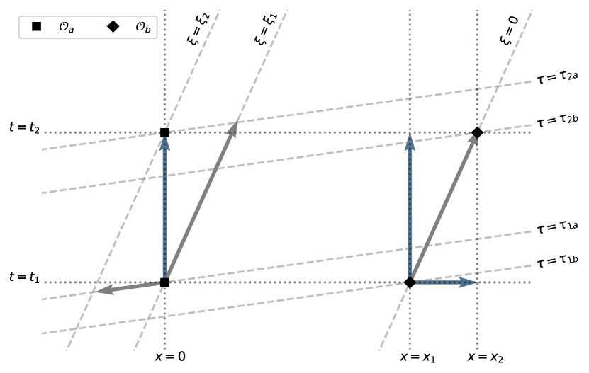
Figure 1. The relative motion of $\mathcal{O}_{a}$ and $\mathcal{O}_{b}$ and the coordinate displacements this defines in the reference frames $K_{a}$ and $K_{b}$.

Figure 1 illustrates point-like observers $\mathcal{O}_{a}$ and $\mathcal{O}_{b}$ with associated rest-frames $K_{a}$ and $K_{b}$, in a state of relative motion. In the frame $K_{a}$ it appears the observer $\mathcal{O}_{b}$ moves between space-time locations $(t_{1},x_{1})$ and $(t_{2},x_{2})$ , while $\mathcal{O}_{a}$ “moves” between locations $(t_{1},0)$ and $(t_{2},0)$. On the other hand the observer $\mathcal{O}_{b}$ is seen to “move” in its rest-frame $K_{b}$ between space-time locations of the form $(\tau_{1b},0)$ and $(\tau_{2b},0)$ while $\mathcal{O}_{a}$ moves between $(\tau_{1a},\xi_{1})$ and $(\tau_{2a},\xi_{2})$. The spatial separation between the points $(t_{1},x_{1})$ and $(t_{2},x_{2})$ is simply not recognised in the rest frame of $\mathcal{O}_{b}$ in the relational framework. On the contrary, the locations $x=x_{1}$ and $x=x_{2}$ are made discernible only because the material point $\mathcal{O}_{b}$ is observed to move between these locations.

Furthermore the instants $t=t_{1}$ and $t=t_{2}$ are made discernible only by the changing location of $\mathcal{O}_{b}$ with respect to $\mathcal{O}_{a}$. Indeed it is such material re-configurations which allow for the measurement of time intervals in practice. For instance, the motion of a sprinter between two fixed positions on a race-track is compared to the number of periodic vibrations of a quartz crystal, typically oscillating at $2^{15}$ Hz in modern watches. The relational viewpoint suggests that the instants $t=t_{1}$ and $t=t_{2}$ have no intrinsic separation (or indeed meaning) without reference to the observed motion of $\mathcal{O}_{b}$ between the locations $x=x_{1}$ and $x=x_{2}$.

The distinction between instants $t_{1}$ and $t_{2}$ and the spatial locations $x_{1}$ and $x_{2}$ is made discernible only because the observer $\mathcal{O}_{b}$ has been observed to move between these space-time locations. Likewise, the distinction between the locations $(\tau_{1b},0)$ and $(\tau_{2b},0)$ in $K_{b}$ is made physical only because $\mathcal{O}_{a}$ is observed to move between locations $(\tau_{1a},\xi_{1})$ and $(\tau_{2a},\xi_{2})$, which are themselves made discernible in $K_{b}$ only because of the observed motion of $\mathcal{O}_{a}$. In particular, it is clear that space-time locations in the frames $K_{a}$ and $K_{b}$ only become physically manifest by the reconfiguration of material observers $\mathcal{O}_{a}$ and $\mathcal{O}_{b}$. This in turn implies that each location in $(t,x)\in K_{a}$ becomes physically manifest only if it has a counterpart $(\tau,\xi)\in K_{b}$, and vice-versa.

On the other hand, it is understood that the coordinate differences in each frame of reference serve to characterise the relative motion, for instance it is the coordinate difference $(t_{2}-t_{1},x_{2}-x_{1})$ which serve to define the velocity and related energy-momentum of $\mathcal{O}_{b}$ with reference to $K_{a}$. It is these coordinate differences and their transformation between reference frames which contains all physical information about the system of observers $\mathcal{O}_{a}$ and $\mathcal{O}_{b}$. In other words, the space-time locations labelled by $K_{a}$ and $K_{b}$ are not in themselves fundamental, however, the transformation of coordinate differences from one reference frame to another is fundamental.

1.2. Relativity and de Broglie waves

It is assumed the observer $\mathcal{O}_{b}$ moves with reference to $K_{a}$ at constant velocity $v=\beta c$, where $\beta\in(-1,1)$ and $c$ is the speed of light. The coordinate map $\bm{\Xi}:K_{a}\to K_{b}$ takes the form

(1) $$\tau=\gamma\left(t-\frac{\beta}{c}x\right)\quad\xi=\gamma\left(x-c\beta t\right);\quad\gamma=\frac{1}{\sqrt{1-\beta^{2}}}.$$

The point emphasised by de Broglie [7, 8] is $\mathcal{O}_{b}$ has an associated angular frequency

(2) $$\omega_{0}=\frac{E_{0}}{\hbar},$$

which may be obtained from the Planck and Einstein relations $E=\hbar\omega$ and $E_{0}=mc^{2}$, where $m$ is the rest mass of $\mathcal{O}_{b}$.

Given this angular frequency, de Broglie postulated that the wave-form $\psi(\tau,\xi)=e^{i\omega_{0}\tau}$ is naturally associated with the observer $\mathcal{O}_{b}$. Meanwhile (1) ensures this wave-form with respect to $K_{a}$ is of the form

(3) $$\psi(t,x)=e^{i\omega_{0}\gamma\left(t-\frac{\beta}{c}x\right)}=e^{i(\omega t-kx)},$$

where $\omega=\gamma\omega_{0}$ and $k=\frac{\omega_{0}\beta\gamma}{c}=\frac{\beta}{c}\omega$. The relativistic energy and momentum of $\mathcal{O}_{b}$ with reference to $K_{a}$ are given by $E=mc^{2}\gamma$ and $p=mc\beta\gamma$, and as such the wave-form $\psi(t,x)$ may be also written as

(4) $$\psi(t,x)=e^{i(\omega t-kx)}:=e^{\frac{i}{\hbar}(Et-px)}.$$

Thus the relativistic energy-momentum $(E,p)$ of the observer $\mathcal{O}_{b}$ are related to the angular frequency $\omega$ and wave-number $k$ of the associated wave-form $\psi$.

A point of importance for de Broglie was that the wave form $\psi(t,x)$ is always in phase with a clock of period $T_{0}=\frac{2\pi}{\omega_{0}}=\frac{mc^{2}}{\hbar}$ at rest in the frame $K_{b}$. This clock is shown in Figure 2 as an oscillator moving along the $y$-axis of the frame $K_{b}$ with angular frequency $\omega_{0}$.

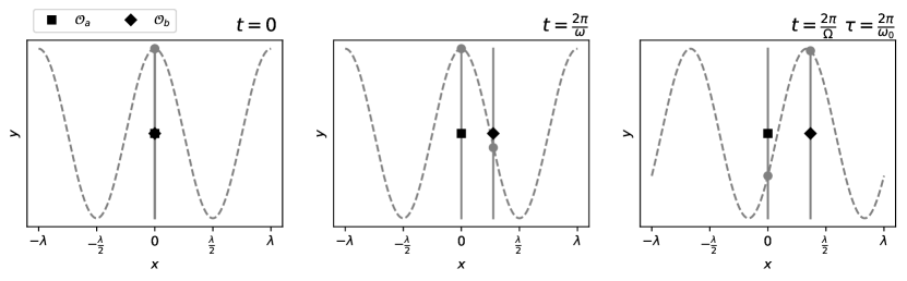
Figure 2. Snapshots of the relative motion of $\mathcal{O}_{a}$ and $\mathcal{O}_{b}$, their local clocks with frequencies $\omega$ and $\omega_{0}$ and the wave-form $\psi(t,x)=\cos(\omega t-kx)$. A related animation may be found at: de Broglie wave animation

The period and angular frequency of this clock relative to $K_{a}$ are

(5) $$T=\gamma T_{0}\quad\Omega=\frac{2\pi}{T}=\frac{\omega_{0}}{\gamma}.$$

The angular frequency $\Omega$ is not to be confused with the angular frequency of $\psi(t,x)$ which is $\omega=\gamma\omega_{0}$ and for reference Figure 2 also shows a similar clock at rest in $K_{a}$ with angular frequency $\omega$.

The clock co-moving with $\mathcal{O}_{b}$ moving between $(t,x)$ and $(t+\differential t,x+\beta c\differential t)$ in $K_{a}$ will undergo a phase-shift $\differential\Phi=\Omega\differential t=\frac{\omega_{0}}{\gamma}\differential t$. Meanwhile, the phase difference of the wave $\psi(t,x)$, between $(t,x)$ and $(t+\differential t,x+\beta cdt)$ is

(6) $$\omega_{0}\gamma\left(dt-\frac{\beta}{c}\beta cdt\right)=\frac{\omega_{0}}{\gamma}\differential t=\differential\Phi,$$

so the moving clock and wave-form $\psi(t,x)$ are in phase, see Figure 2. It is clear then that de Broglie waves are closely connected with the Lorentz transformation between local inertial reference frames $K_{a}$ and $K_{b}$, in particular with the coordinate map $\tau(t,x)$. The aim now is derive the existence of such a wave-form as a representation of this coordinate map between the rest-frames of the observers $\mathcal{O}_{a}$ and $\mathcal{O}_{b}$.

2. Coordinate maps and their governing equations

2.1. Motion and coordinate maps

At any instant of its motion through $K_{a}$, the observer $\mathcal{O}_{b}$ is following a trajectory with tangent vector $(\differential{t},\differential{x})$, while the corresponding trajectory with reference to $K_{b}$ is of the form $(\differential{\tau},0)$. Correspondingly, the observer $\mathcal{O}_{a}$ must be travelling along a trajectory in $K_{b}$ whose tangent vector is of the form $(\differential{\tau},\differential{\xi})$, while this tangent vector has counterpart $(\differential{t},0)$ with reference to $K_{a}$, cf. Figure 1.

In general, coordinate differences $(\differential{\tau},\differential{\xi})$ with reference to $K_{b}$ are related to their counterparts $(\differential{t},\differential{x})$ with reference to $K_{a}$ according to

$$\begin{bmatrix}\differential{\tau}\\ \differential{\xi}\end{bmatrix}=\begin{bmatrix}\tau_{t}&\tau_{x}\\ \xi_{t}&\xi_{x}\end{bmatrix}\begin{bmatrix}\differential{t}\\ \differential{x}\end{bmatrix}\qquad\begin{bmatrix}\differential{t}\\ \differential{x}\end{bmatrix}=\begin{bmatrix}t_{\tau}&t_{\xi}\\ x_{\tau}&x_{\xi}\end{bmatrix}\begin{bmatrix}\differential{\tau}\\ \differential{\xi}\end{bmatrix},$$

where sub-scripts denote differentiation with respect to the relevant variable. To ensure consistency with the special theory of relativity, it is required that tangent vectors of the form $(\differential{t},\beta c\differential{t})$, $(\differential{t},0)$ and $(\differential{t},c\differential{t})$ have counterparts $(\differential{\tau},0)$, $(\differential{\tau},-\beta c\differential{\tau})$ and $(\differential{\tau},c\differential{\tau})$ respectively. This requires the Jacobian matrices of the coordinate maps to be of the form

(7) $$\begin{bmatrix}\differential{\tau}\\ \differential{\xi}\end{bmatrix}=\begin{bmatrix}\tau_{t}&\tau_{x}\\ c^{2}\tau_{x}&\tau_{t}\end{bmatrix}\begin{bmatrix}\differential{t}\\ \differential{x}\end{bmatrix}\iff\begin{bmatrix}\differential{t}\\ \differential{x}\end{bmatrix}=\begin{bmatrix}t_{\tau}&\frac{1}{c^{2}}x_{\tau}\\ x_{\tau}&t_{\tau}\end{bmatrix}\begin{bmatrix}\differential{\tau}\\ \differential{\xi}\end{bmatrix},$$

In addition it is required that the Jacobian of each coordinate map should satisfy

(8) $$J=\tau_{t}^{2}-c^{2}\tau_{x}^{2}=t_{\tau}^{2}-\frac{1}{c^{2}}x_{\tau}^{2}=1$$

2.2. The Hamilton-Jacobi Equations

The action for the coordinate map $\mathbf{X}:K_{b}\to K_{a}$, associated with the motion $(t_{1},x_{1})\to(t,x)$ induced by the motion of $\mathcal{O}_{b}$ along the corresponding trajectory $(\tau_{1},0)\to(\tau,0)$ is given by

(9) $$S[\underline{x}]=\frac{E_{0}}{2c^{2}}\int_{\tau_{1}}^{\tau}\underline{x}_{\tau}.\underline{x}_{\tau}\differential{\tau}=\int_{\tau_{1}}^{\tau}L[\underline{x},\underline{x}_{\tau}]\differential{\tau}.$$

The notation means $\underline{x}(\tau)\equiv\left(ct(\tau,0),x(\tau,0)\right)\in K_{a}$ which is the image of the map $\mathbf{X}:K_{b}\to K_{a}$ applied to the trajectory $\underline{\xi}(\tau)\equiv\left(\tau,0\right)\in K_{b}$. The inner-product is given by

$$\underline{x}_{\tau}.\underline{x}_{\tau}=c^{2}t_{\tau}^{2}-x_{\tau}^{2}=c^{2}J$$

where $J$ is the Jacobian of the coordinate map $\mathbf{X}:K_{b}\to K_{a}$ (cf. equation (8)). The constraint $J=1$ is interpreted as a weak equation, to be applied after variational derivatives are calculated, in line with the terminology of Dirac (cf. [9]).

Under a variation of the form $\underline{x}(\tau)\to\underline{x}(\tau)+\epsilon\underline{u}(\tau)$, Hamilton’s principle is simply the requirement $\evaluated{\frac{d}{d\epsilon}S[\underline{x}+\epsilon\underline{u}]}_{\epsilon=0}=0,$ and can be written for a general Lagrangian $L[\underline{x},\underline{x}_{\tau}]$ according to

(10) $$\int_{\tau_{1}}^{\tau}\left[\frac{\partial L}{\partial\underline{x}}-\derivative{\tau}\frac{\partial L}{\partial\underline{x}_{\tau}}\right].\underline{u}\differential{\tau}+\int_{\tau_{1}}^{\tau}\derivative{\tau}\left(\partialderivative{L}{\underline{x}_{\tau}}.\underline{u}\right)\differential{\tau}=0$$

after integration by parts. Imposing the boundary conditions $\underline{u}(\tau_{1})=\underline{u}(\tau_{b})=\underline{0}$ to an otherwise arbitrary variation $\underline{u}(\tau)$, yields the Euler-Lagrange equations

(11) $$\frac{\partial L}{\partial\underline{x}}-\frac{d}{d\tau}\frac{\partial L}{\partial\underline{x}_{\tau}}=\underline{0}.$$

When $L=\frac{E_{0}}{2c^{2}}\left(c^{2}t_{\tau}^{2}-x_{\tau}^{2}\right)$ specifically, the Euler-Lagrange equations for the coordinate map $\mathbf{X}:K_{b}\to K_{a}$ satisfies $\derivative[2]{\tau}\mathbf{X}(\tau,0)=0$.

The Hamilton-Jacobi equation follow from the condition $\underline{x}(\tau)$ is a physical path (i.e. satisfying (11)), while the variation is now required to satisfy $\underline{u}(\tau_{1})=\underline{0}$ only, while $\underline{u}(\tau)$ may be arbitrarily chosen. The variation of the action under this perturbation is obtained from (10)

(12) $$\lim_{\epsilon\to 0}\frac{S[\underline{x}+\epsilon\underline{u}]-S[\underline{x}]}{\epsilon\underline{u}}=\frac{\partial S}{\partial\underline{x}}=\frac{\partial L}{\partial\underline{x}_{\tau}}.$$

The canonical energy-momentum associated with the trajectory of $\mathcal{O}_{b}$, with reference to the frame $K_{a}$, is given by

(13) $$\begin{cases}\partialderivative{S}{t}&=E_{p}=E_{0}t_{\tau}\implies t_{\tau}=\frac{E_{p}}{E_{0}}\\ \partialderivative{S}{x}&=-p=\frac{E_{0}}{c^{2}}x_{\tau}\implies{x}_{\tau}=\frac{c^{2}p}{E_{0}}\end{cases}$$

The Hamiltonian associated with coordinate map $\mathbf{X}:K_{b}\to K_{a}$ along $(\tau,0)$ is

$$H=\underline{p}.\underline{x}_{\tau}-L=\frac{E_{p}^{2}-c^{2}p^{2}}{2E_{0}},$$

which of course is conserved.

Upon imposing the constraint $J=1$, it follows that

(14) $$\left(\frac{\partial S}{\partial t}\right)^{2}-c^{2}\left(\frac{\partial S}{\partial x}\right)^{2}=E_{0}^{2}.$$

Conservation of energy-momentum in the form $\frac{1}{c^{2}}\partial_{t}E_{p}+\partial_{x}p=0$ or equivalently

(15) $$\partialderivative[2]{S}{t}-c^{2}\partialderivative{S}{x}=0,$$

is consistent with this constraint, since $\partial_{t}\frac{\partial S}{\partial t}=\partial_{t}\frac{\partial L}{\partial t_{\tau}}=\frac{\partial^{2}L}{\partial t\partial t_{\tau}}=0$ and likewise for $\frac{\partial^{2}S}{\partial x^{2}}$.

Upon using the relations (13) and the constraint (14), we also find

(16) $$\frac{dS}{d\tau}=\frac{\partial S}{\partial t}t_{\tau}+\frac{\partial S}{\partial x}\cdot x_{\tau}=E_{0},$$

and so integrating with respect to $\tau$ yields $S[\underline{x}]=E_{0}\tau(\underline{x})$ up to an additive constant. Given $S[\underline{x}]=E_{0}\tau(\underline{x})$, it follows the system (14)–(15) governing the action $S[t,x]$ also governs the component $\tau(t,x)$ of the coordinate map $\bm{\Xi}:K_{a}\to K_{b}$, which similarly satisfies

(17a) $$\partial_{t}^{2}\tau-c^{2}\partial_{x}^{2}\tau =0$$

(17b) $$(\partial_{t}\tau)^{2}-c^{2}(\partial_{x}\tau)^{2} =1.$$

Solutions of the system (17a)–(17b) will form representations of the coordinate map $\tau(t,x)$.

3. Coordinate maps and their representations

3.1. Linearity of the coordinate maps

The main result of this section is that the system (14)–(15) only admits solutions $S[t,x]$ which are linear in $t$ and $x$. However, it will also be shown that $S$ as a solution of (17a)–(17b) may be represented as an exponential function of $t$ and $x$ (cf. [14]).

Without imposing assumptions or restrictions, we consider a general solution of the form

(18) $$S(t,x)=E_{0}\Theta(\psi(t,x)),$$

where $\Theta(\psi(t,x))=\tau(t,x)$ with $\psi(t,x)$ being a representation of $\tau(t,x)$. Substituting (18) into the governing equations (14)–(15) yields

(19a) $$\left[\partial_{t}^{2}\psi-c^{2}\partial^{2}_{x}\psi\right]\Theta^{\prime}(\psi)+\left[\left(\partial_{t}\psi\right)^{2}-c^{2}\left(\partial_{x}\psi\right)^{2}\right]\Theta^{\prime\prime}(\psi)=0$$

(19b) $$\left[\left(\partial_{t}\psi\right)^{2}-c^{2}\left(\partial_{x}\psi\right)^{2}\right]\Theta^{\prime}(\psi)^{2}=1,$$

where $\Theta^{\prime}(\psi)=\derivative{\Theta}{\psi}$.

Equation (19b) applied to equation (19a) now yields

(20) $$\partial^{2}_{t}\psi-c^{2}\partial^{2}_{x}\psi+\frac{\Theta^{\prime\prime}(\psi)}{\Theta^{\prime}(\psi)^{3}}=0.$$

Multiplying by $\partial_{t}\psi$, it now follows that

(21) $$\frac{1}{2}\partial_{t}\left[(\partial_{t}\psi)^{2}-\frac{1}{\Theta^{\prime}(\psi)^{2}}\right]-c^{2}\partial^{2}_{x}\psi\partial_{t}\psi=0,$$

while substituting from equation (19b) we deduce

$$\partial_{x}\psi\partial_{x}\partial_{t}\psi-\partial_{t}\psi\partial_{x}^{2}\psi=0$$

from which it follows $\partial_{x}\left(\frac{\partial_{x}\psi}{\partial_{t}\psi}\right)=0$. Multiplying equation (20) by $\partial_{x}\psi$ we also deduce $\partial_{t}\left(\frac{\partial_{x}\psi}{\partial_{t}\psi}\right)=0,$ and as such $\frac{\partial_{x}\psi}{\partial_{t}\psi}$ is constant.

This means the functions $\partial_{t}\psi$ and $\partial_{x}\psi$ are linearly dependent. It follows that $\psi$ may be written according to

$$\psi(t,x)=\phi(\omega t-kx)\implies\frac{\partial_{x}\psi}{\partial_{t}\psi}=-\frac{k}{\omega},$$

where $\phi(\cdot)$ is yet to be determined while $\omega$ and $k$ are constants. The constraint (17b) or equivalently (19b) now requires

(22) $$\left(\omega_{0}\derivative{\phi}{s}\derivative{\Theta}{\phi}\right)^{2}=1,\quad\omega_{0}^{2}=\omega^{2}-c^{2}k^{2}>0,$$

where we introduce $s=\omega t-kx$. Taking the square-root of (22) we now have $\pm\omega_{0}\derivative{\phi}{s}\derivative{\Theta}{\phi}=1$ and so integrating it follows that $\Theta(\phi(s))=\pm\frac{s}{\omega_{0}}$, or equivalently

(23) $$\tau(t,x)=\Theta(\psi(t,x))=\pm\frac{\omega t-kx}{\omega_{0}}.$$

Formally, we have applied the inverse function theorem to equation (22) which ensures $\pm\omega_{0}\Theta(\cdot)=\phi^{-1}(\cdot)$ (see [18] for instance). It also follows from (13) and (23) with $S=E_{0}\tau$ that

(24) $$\begin{cases}\partialderivative{S}{t}=E\implies\frac{\omega}{\omega_{0}}=\frac{E}{E_{0}}\\ \partialderivative{S}{x}=-p\implies\frac{k}{\omega_{0}}=\frac{p}{E_{0}}.\end{cases}$$

3.2. Representations of the coordinate map

As a functional equation for $\Theta(\phi)$, we note that under the re-scaling $\phi\to r\phi$ for a non-zero constant $r$, equation (22) also requires

(25) $$r^{2}\Theta^{\prime}(r\phi)^{2}\dot{\phi}(s)^{2}=\Theta^{\prime}(\phi)^{2}\dot{\phi}(s)^{2}=1.$$

It follows $r^{2}\Theta^{\prime}(r\phi)^{2}$ is independent of $r$ and so $\Theta^{\prime}(r\phi)\propto\frac{1}{r\phi}$ from which it follows

(26) $$E_{0}\Theta(\psi(t,x))=\alpha\ln\psi=\pm E_{0}\frac{\omega t-kx}{\omega_{0}},$$

where $\alpha$ is a constant action parameter. The representation $\psi(t,x)$ of the coordinate map $\tau(t,x)$ is now explicitly:

(27) $$\psi(t,x)=e^{\pm\frac{1}{\alpha}(Et-px)},$$

having used equation (24) to re-write the ratios $\frac{E_{0}\omega}{\omega_{0}}=E$ and $\frac{E_{0}k}{\omega_{0}}=p$.

The other possible solution of (22) is simply

(28) $$\begin{rcases}\phi(s)=\kappa s\\ \omega_{0}\Theta(\phi)=\pm\frac{\phi}{\kappa}\end{rcases}\implies\Theta(\phi(s))=\pm\frac{s}{\omega_{0}}$$

where $\kappa$ is constant, thereby ensuring $\derivative[2]{\phi}{s}=0$ and $\derivative[2]{\Theta}{\phi}=0$. This in turn ensures (19a) is satisfied while (19b) is satisfied by definition of $\omega_{0}$ and $s$.

3.3. Momentum measurement & de Broglie waves

In §§3.1–3.2 it has been shown that the coordinate map $S=E_{0}\tau(t,x)$ governed by (17b)–(17a), is necessarily linear $E_{0}\tau(t,x)=\pm(Et-px)$ and has a representation of the form $E_{0}\tau(t,x)=\alpha\ln\psi(t,x)$. Combining these observations then it is necessary that the representation $\psi(t,x)$ is of the form

$$\psi(t,x)=\exp{\pm\frac{1}{\alpha}(Et-kx)}.$$

It is already clear $\alpha$ must have the units of action, so the choice $\hbar$ is obvious. To ensure the representation $\psi(t,x)$ corresponds to a de Broglie wave of the form (4), it is also necessary to show $\alpha$ is imaginary, which is the aim of the current section.

Figure 3 shows a very simple apparatus consisting of two massive plates $\mathcal{P}_{l}$ and $\mathcal{P}_{r}$, both initially static at $x_{l}=0$ and $x_{r}=\lambda$ with reference to the frame $K$, with rest energy $\mathscr{E}_{0}$ each. It is supposed the point-like observer $\mathcal{O}_{b}$ is located at some $x\in(x_{l},x_{r})$, and interacts with either plate only by collision. Upon collision $\mathcal{O}_{b}$ undergoes a change of momentum, thereby imparting momentum to one of these plates.

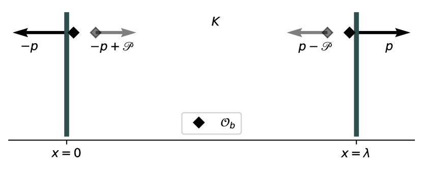
Figure 3. The measurement of $\mathcal{O}_{b}$’s momentum by collision with massive plates of equal rest-energy $\mathscr{E}_{0}$.

Measurement of momentum means $\mathcal{O}_{b}$ impacts one of the plates and sets it in motion relative to the other. Immediately after impact the plates are again inertial observers, since there is no further interaction to impart momentum to either plate.

If $K_{l}\owns(t^{\prime},x^{\prime})$ denotes the rest-frame of $\mathcal{P}_{l}$, then its coordinates with reference to this frame will always be of the form $\left(t^{\prime},0\right)$; those of $\mathcal{P}_{r}$ will be of the form $(t^{\prime},\lambda)$ prior to collision. Similarly, $K_{r}\ni(t^{*},x^{*})$ is the rest-frame of $\mathcal{P}_{r}$ whose coordinates are always of the form $\left(t^{*},0\right)$; those of $\mathcal{P}_{l}$ are of the form $(t^{*},-\lambda)$ initially. Prior to collision it makes sense to identify coordinates $(t,x)\in K$, $(t^{\prime},x^{\prime})\in K_{l}$ and $(t^{*},x^{*})\in K_{r}$ since all three frames see the observers $\mathcal{P}_{l}$ and $\mathcal{P}_{r}$ at rest, and so all are equivalent up to constant translations.

At the moment of measurement as observed from the frame $K_{l}$, it appears the observer $\mathcal{P}_{r}$ changes energy-momentum according to $(\mathscr{E}_{0},0)\to(\mathscr{E},\mathscr{P})$ where $\mathscr{E}^{2}=\mathscr{P}^{2}c^{2}+\mathscr{E}_{0}^{2}$ and $\mathscr{P}>0$ is assumed. Meanwhile the momentum of $\mathcal{O}_{b}$ changes according to $(E,p)\to(E_{1},p-\mathscr{P})$ (cf. Figure 3). Naturally, the energy-momentum of $\mathcal{P}_{l}$ is always $(\mathscr{E}_{0},0)$ in the frame $K_{l}$ while the observer $\mathcal{O}_{b}$ is interpreted to occupy the location $x^{\prime}=\lambda$ upon collision. Conversely, in the frame $K_{r}$ the observer $\mathcal{P}_{l}$ changes its energy-momentum according to $(\mathscr{E}_{0},0)\to(\mathscr{E},-\mathscr{P})$ and the energy-momentum of $\mathcal{O}_{b}$ changes according to $(E,-p)\to(E_{1},-p+\mathscr{P})$. In this frame of reference the observer $\mathcal{O}_{b}$ is interpreted to appear at $x^{*}=-\lambda$ upon impact, and by definition the energy-momentum of $\mathcal{P}_{r}$ is always $(\mathscr{E}_{0},0)$.

Given that $\mathcal{P}_{l}$ and $\mathcal{P}_{r}$ are in uniform relative motion before and after collision with $\mathcal{O}_{b}$, it follows from §3.2 the component $t^{*}(t^{\prime},x^{\prime})$ of the coordinate map $\mathbf{X^{*}}:K_{l}\to K_{r}$ has representation

$$\psi(t^{\prime},x^{\prime})=\begin{cases}e^{\frac{1}{\alpha}\mathscr{E}_{0}(t^{\prime}-t^{\prime}_{0})},\quad t^{\prime}<t^{\prime}_{0}\\ e^{\frac{1}{\alpha}\left(\mathscr{E}(t^{\prime}-t^{\prime}_{0})-\mathscr{P}x^{\prime}\right)}\quad t^{\prime}\geq t^{\prime}_{0}\end{cases}$$

where the impact occurs at time $t^{\prime}_{0}$ with reference to $K_{l}$. Upon impact the proper-time $t^{*}$ of the observer $\mathcal{P}_{r}$ changes according to

$$\frac{\alpha}{\mathscr{E}_{0}}\ln e^{\frac{1}{\alpha}\mathscr{E}_{0}(t^{\prime}-t^{\prime}_{0})}\to\frac{\alpha}{\mathscr{E}_{0}}\ln e^{\frac{1}{\alpha}\left(\mathscr{E}(t^{\prime}-t^{\prime}_{0})-\mathscr{P}x^{\prime}\right)},$$

from the perspective of the observer $\mathcal{P}_{l}$. However, according to the observer $\mathcal{P}_{r}$ its own time coordinate is continuous, while it is the time coordinate of $\mathcal{P}_{l}$ which undergoes a corresponding change during collision with $\mathcal{O}_{b}$. Continuity of the $t^{*}$-coordinate now requires

(29) $$\lim_{t^{\prime}\to t^{\prime}_{0}}e^{\frac{1}{\alpha}\mathscr{E}_{0}(t^{\prime}-t^{\prime}_{0})}=\lim_{t^{\prime}\to t^{\prime}_{0}}e^{\frac{1}{\alpha}\left(\mathscr{E}(t^{\prime}-t^{\prime}_{0})-\mathscr{P}\lambda\right)}\iff e^{-\frac{\mathscr{P}\lambda}{\alpha}}=1.$$

Since $\lambda\neq 0$ and $\mathscr{P}>0$ by assumption, continuity of $\psi(t,x)$ at $t^{\prime}_{0}$ is satisfied only when the argument of the exponential is of the form $2\pi ni$ for $n\in\mathbb{Z}$. Hence, we deduce

$$\alpha=-i\hbar,\quad\mathscr{P}=\frac{2\pi n\hbar}{\lambda},$$

and so the action parameter $\alpha$ is imaginary as anticipated.

With $\alpha=-i\hbar$ it is now clear that the coordinate transformation between the rest frames of inertial observers may be represented by wave-forms

(30) $$\psi(t,x)=e^{\frac{i}{\hbar}\left(E_{p}t-px\right)},$$

whose eigenvalues may be defined as

(31) $$E_{p}=\bar{\psi}(-i\hbar\partial_{t})\psi\qquad p=\bar{\psi}(i\hbar\partial_{x})\psi,$$

where $\bar{\psi}$ denotes the complex conjugate of $\psi$. Both representations $\psi$ and $\bar{\psi}$ satisfy the Klein-Gordon equation

(32) $$\frac{1}{c^{2}}\partialderivative[2]{\psi}{t}-\partialderivative[2]{\psi}{x}+\frac{m^{2}c^{2}}{\hbar^{2}}\psi=0.$$

Thus, de Broglie waves as per Dirac’s terminology (see [10], p. 120) emerge as a representation of the $\tau$-component of the coordinate map $\bm{\Xi}:K_{a}\to K_{b}$, and so represents to trajectory of $\mathcal{O}_{b}$ (i.e. $(\tau,0)\in K_{b}$ with reference to $K_{a}$.

The existence of de Broglie waves was confirmed almost immediately after de Broglie’s first prediction [7], with the interference experiments of Davisson & Germer [6] and the contemporaneous experiments of Thomson & Reid [21]. In the years since, the experimental evidence supporting de Broglie’s conjecture has accumulated steadily (see [1, 19, 20] among others).

3.4. Energy-momentum eigenfunctions

The $\tau$-representation given in equation (30) is an eigenfunction of the linear operators $-i\hbar\partial_{t}$ and $i\hbar\partial_{x}$, whose corresponding eigenvalues are simply the energy-momentum of the observer $\mathcal{O}_{b}$ with reference to the frame $K_{a}$. The nonlinear constraint (17b) has a particularly elegant geometric interpretation in the relational context, since one may reformulate the coordinate map (7) according to

(33) $$\begin{bmatrix}d\tau\\ d\xi\end{bmatrix}=\begin{bmatrix}\tau_{t}&\tau_{x}\\ \xi_{t}&\xi_{x}\end{bmatrix}\begin{bmatrix}dt\\ dx\end{bmatrix}=\begin{bmatrix}\tau_{t}&\tau_{x}\\ c^{2}\tau_{x}&\tau_{t}\end{bmatrix}\begin{bmatrix}dt\\ dx\end{bmatrix}$$

in which case $\tau_{t}^{2}-c^{2}\tau_{x}^{2}=1$ is equivalent to $\det\begin{bmatrix}\tau_{t}&\tau_{x}\\ \xi_{t}&\xi_{x}\end{bmatrix}=1.$

Hence, the Jacobian of the coordinate transformation $\bm{\Xi}:K_{a}\to K_{b}$ is required to be one, thus ensuring this map is invertible. Specifically, it means that a trajectory $(\differential{t},\differential{x})$ in $K_{a}$ has as counterpart $(\differential{\tau},\differential{\xi})$ with reference to $K_{b}$ and vice-versa. In particular it means that a trajectory of $\mathcal{O}_{b}$ in $K_{b}$ given by $(\differential{\tau},0)$ has a counterpart $(\differential{t},\differential{x})$ in $K_{a}$, while simultaneously the trajectory of $\mathcal{O}_{a}$ in $K_{a}$ given by $(\differential{t},0)$ has a counterpart $(\differential{\tau},\differential{\xi})$ in $K_{b}$, cf. Figure 1. As such, these observers appear as point-like bodies moving with reference to the rest-frame of their counterpart (cf. Figure 1). This is only possible since the conditions (17a)–(17b) are both satisfied for the coordinate map $E_{0}\tau(t,x)=-i\hbar\ln\psi(t,x)$ when $\psi(t,x)$ is an energy-momentum eigenfunction.

Contrarily, given the linearity of (32) it is clear that superpositions of the form $\varphi(t,x)=\iint\delta(E^{2}-E_{p}^{2})a(E,p)e^{\frac{i}{\hbar}(Et-px)}dEdp$ are also valid solutions of this wave equation. Such a superposition cannot represent a physically realisable coordinate map from $K_{a}$ to $K_{b}$ since the non-linear constraint (17b) is not satisfied for $-i\hbar\ln\varphi$. This is not to say $\mathcal{O}_{b}$ becomes somehow de-localised, it always has a precise location $(\tau,0)\in K_{b}$. Rather, it is the case there is no longer a precise correspondence of the form (7) between the frames $K_{a}$ and $K_{b}$, and so the trajectory $(\differential{\tau},0)$ in $K_{b}$ no longer has a precise counterpart with reference to $K_{a}$ satisfying all the required axioms of special relativity.

4. Discussion

A central point of the argument in §3.3 is that the observers $\mathcal{P}_{l}$ and $\mathcal{P}_{r}$ are both always inertial in their own rest-frames, and the acceleration of the pair upon impact with $\mathcal{O}_{b}$ is only defined in relative terms. This is apparently consistent only in the relational space-time framework. Moreover, the derivation presented here appears to be consistent with Rovelli’s Relational Quantum Mechanics (RQM) [15, 17], whereby the properties of a system are not absolutes. In particular, the perceived location and momentum of $\mathcal{O}_{b}$ upon impact with the apparatus depends on the frame of reference adopted for the measurement.

Indeed the physical properties of a system, in this case the energy-momentum of $\mathcal{P}_{l}$ and $\mathcal{P}_{r}$, is a characteristic of interaction between the observers, specifically it is a property of the coordinate maps between their respective rest-frames (cf. [12]). It is also clear the observer $\mathcal{O}_{b}$ does not have an absolute location in this experiment, its apparent location is contingent on the frame of reference used for the observation. Thus the derivation presented here also appears to lend support to Rovelli’s hypothesis (see [16] pp. 220–221) that the relational character of states in RQM is connected to the relational framework of space and time.

Declarations

Conflicts of Interest

The author declares there are no conflicts of interest, financial or otherwise, related to this work.

Funding

No funding was obtained for the preparation of this manuscript.

References

• [1] Arndt, M, Nairz, O, Vos-Andreae, J, Keller, C, VanΒ der Zouw, G, and Zeilinger, A. Wave–particle duality of $\mathrm{{C}_{60}}$ molecules. Nature, 401:680–682, 1999.
• [2] Barbour, JΒ B. Relative-distance Machian theories. Nature, 249:328–329, 1974.
• [3] Barbour, JΒ B. Relational concepts of space and time. Brit. J. Philos. Sci., 33:251–274, 1982.
• [4] Barbour, JΒ B and Bertotti, B. Gravity and inertia in a Machian framework. Nuovo Ciment. B, 38:1–27, 1977.
• [5] Barbour, JΒ B and Bertotti, B. Mach’s principle and the structure of dynamical theories. Proc. R. Soc. Lon. Ser. A., 382:295–306, 1982.
• [6] Davisson, C and Germer, LΒ H. The scattering of electrons by a single crystal of nickel. Nature, 119:558–560, 1927.
• [7] deΒ Broglie, L. Recherches sur la thΓ©orie des quanta. In Ann. de Phys., volumeΒ 10, pages 22–128, 1925. Translation by A F Kraklauer (2004).
• [8] deΒ Broglie, L. An Introduction to the Study of Wave Mechanics. Methuen & Co., London, 1930.
• [9] Dirac, P AΒ M. Lectures on Quantum Mechanics. Belfer Graduate School of Science, Yeshiva University, New York, 1964.
• [10] Dirac, P AΒ M. The Principles of Quantum Mechanics. Oxford University Press, Oxford, 2007.
• [11] Leibniz, GΒ W and Clarke, S. Leibniz and Clarke: Correspondence. Hackett Publishing, 2000. Edited by: Ariew, R.
• [12] Loveridge, L, Miyadera, T, and Busch, P. Symmetry, reference frames, and relational quantities in quantum mechanics. Found. Phys., 48:135–198, 2018.
• [13] Minkowski, H. Space and time. In Space and Time: Minkowski’s Papers on Relativity, pages 39–54. Minkowski Institute Press, Montreal, 2012.
• [14] Motz, L and Selzer, A. Quantum mechanics and the relativistic Hamilton-Jacobi equation. Phys. Rev., 133:B1622, 1964.
• [15] Rovelli, C. Relational quantum mechanics. Int. J. Theor. Phys., 35:1637–1678, 1996.
• [16] Rovelli, C. Quantum Gravity. Cambridge University Press, 2004.
• [17] Rovelli, C. Space is blue and birds fly through it. Philos. Trans. Royal Soc. A, 376:20170312, 2018.
• [18] Rudin, W. Principles of Mathematical Analysis, volumeΒ 3. McGraw-Hill, New York, 1976.
• [19] Schmidt, HΒ T, Fischer, D, Berenyi, Z, Cocke, CΒ L, Gudmundsson, M, Haag, N, Johansson, H AΒ B, KΓ€llberg, A, Levin, SΒ B, Reinhed, P, etΒ al. Evidence of wave-particle duality for single fast hydrogen atoms. Phys. Rev. Lett., 101:083201, 2008.
• [20] Shayeghi, A, Rieser, P, Richter, G, Sezer, U, Rodewald, JΒ H, Geyer, P, Martinez, TΒ J, and Arndt, M. Matter-wave interference of a native polypeptide. Nature Communications, 11:1–8, 2020.
• [21] Thomson, GΒ P and Reid, A. Diffraction of cathode rays by a thin film. Nature, 119:890–890, 1927.