Optimal transport and Wasserstein distances for causal models

Abstract

In this paper we introduce a variant of optimal transport adapted to the causal structure given by an underlying directed graph. Different graph structures lead to different specifications of the optimal transport problem. For instance, a fully connected graph yields standard optimal transport, a linear graph structure corresponds to adapted optimal transport, and an empty graph leads to a notion of optimal transport related to CO-OT, Gromov–Wasserstein distances and factored OT. We derive different characterizations of causal transport plans and introduce Wasserstein distances between causal models that respect the underlying graph structure. We show that average treatment effects are continuous with respect to causal Wasserstein distances and small perturbations of structural causal models lead to small deviations in causal Wasserstein distance. We also introduce an interpolation between causal models based on causal Wasserstein distance and compare it to standard Wasserstein interpolation.

Keywords Optimal transport, causality, directed graphs, causal Wasserstein distance, average treatment effect
MSC 2020 Subject Classification 62H22; 60D99; 90C15; 62H22

1 Introduction

Originally, optimal transport problems were introduced by Monge [43] and, in a more general form, by Kantorovich [34] to study the most efficient way to transport goods from a set of production sites to different destinations. But in addition to this immediate application, optimal transport theory has also lead to the the notion of Wasserstein distance [33, 64, 66], which defines a metric between different probability distributions. Over the years, optimal transport has found applications in different areas of economics [16, 26, 53], probability theory [55, 56] statistics [25, 27, 44], differential geometry [22, 24, 61], robust optimization [10, 42, 69], machine learning and data science [4, 19, 50, 60], just to name a few. At the same time, various variants and extensions of optimal transport have emerged, like multi-marginal versions [2, 23, 47], optimal transport with additional constraints [9, 14, 15, 20, 36, 45], optimal transport between measures with different masses [17, 59], relaxations [12, 39] and regularizations [18, 40]. Causal research examines causal relationships between different events; see e.g. [30, 48, 49, 58]. In probabilistic theories of causality, the underlying causal structure is typically described by a directed graph, leading to graphical causal models [11].

In this paper we introduce a version of optimal transport that is adapted to the causal structure given by an underlying directed graph and investigate corresponding Wasserstein distances between different causal models. The structure of the graph determines the exact specification of the optimal transport problem. A fully connected graph corresponds to standard optimal transport, which consists in finding an optimal transport plan transforming a given distribution into another one. Missing edges translate into additional constraints, which increase the causal Wasserstein distance and therefore, lead to a finer topology on the corresponding set of causal models. For instance, a linear graph requires transport plans to respect the temporal structure. This results in so-called adapted transport problems, which have been studied in [5, 6, 8, 37]. An empty graph restricts transport plans the most and is related to CO-OT problems [62], the Gromov–Wasserstein distance [41] and factored OT [63].

The remainder of this paper is organized as follows: In Section 2 we introduce the setup and provide definitions of causal transport plans together with the corresponding optimal transport problems in Definitions 2.1 and 2.2. In Section 2.4 we showcase the relation to existing concepts of optimal transport from the literature. In Section 3 we focus on causal transport maps for directed acyclic graphs. We derive alternative characterizations of causal transport plans in Theorem 3.4 and Corollary 3.5 and study the structure of sets of causal transport plans in Proposition 3.6. In Section 4 we introduce Wasserstein distances between causal models that respect the structure of the underlying graph. We show that they satisfy all properties of a metric except for the triangle inequality in Proposition 4.3. In Section 4.1, we prove that average treatment effects, which estimate the causal effect of a treatment or intervention, are continuous with respect to causal Wasserstein distance under a change of the underlying probability model while this is not the case for standard Wasserstein distances. On the other hand, in Section 4.2, we show that small perturbations of a structural causal model correspond to small deviations in causal Wasserstein distance. Finally, in Section 4.3 we study a Wasserstein interpolation between causal models that respects the causal structure and compare it to standard Wasserstein interpolation.

2 Notation and definitions

2.1 Causal structures described by directed graphs

We consider a finite set $V=\left\{1,\dots,n\right\}$ for some $n\in\mathbb{N}$, endowed with a causal structure given by a set of directed edges $E\subseteq\{(i,j)\in V\times V:i\neq j\}$. This turns $G=(V,E)$ into a directed graph. For $j\in V$, we denote by $\text{\rm pa}_{j}$ the parents of $j$, given by

$$\text{\rm pa}_{j}:=\{i\in V:(i,j)\in E\},$$

and for a subset $A\subseteq V$, we define

$$\text{\rm pa}_{A}:=\bigcup_{j\in A}\text{\rm pa}_{j}.$$

We order both sets $\text{\rm pa}_{j}$ and $\text{\rm pa}_{A}$ according to the natural ranking of $V=\{1,\dots,n\}$.

If $G$ has no cycles, it is called a directed acyclic graph (DAG). By reordering the vertices, a DAG can always assumed to be sorted, which means that it only contains edges $(i,j)$ such that $i<j$; see e.g. [11, 38, 48].

2.2 Spaces and measures

We consider two product spaces of the form $\mathcal{X}=\mathcal{X}_{1}\times\dots\times\mathcal{X}_{n}$ and $\mathcal{Y}=\mathcal{Y}_{1}\times\dots\times\mathcal{Y}_{n}$ for non-empty Polish spaces ${\cal X}_{i},{\cal Y}_{i}$, $i=1,\dots,n$. We endow $\mathcal{X}$, $\mathcal{Y}$ and $\mathcal{X}\times\mathcal{Y}$ with the product topologies, which makes them again Polish; see e.g. [13, Chapter IX, §6.1, Proposition I]. By $\mathcal{P}(\mathcal{X})$, $\mathcal{P}(\mathcal{Y})$ and $\mathcal{P}(\mathcal{X}\times\mathcal{Y})$ we denote the set of all Borel probability measures on $\mathcal{X}$, $\mathcal{Y}$ and $\mathcal{X}\times\mathcal{Y}$, respectively. If we write $X\sim\mu$ for a measure $\mu\in\mathcal{P}(\mathcal{X})$, we mean that $X$ is an $\mathcal{X}$-valued random variable with distribution $\mu$ defined on some underlying probability space. Moreover, we use the notation $X_{1:i}$ to denote the tuple $(X_{1},\dots,X_{i})$ for $i\in V=\{1,\dots,n\}$, and similarly, $X_{A}$ for any ordered subset $A$ of $V=\{1,\dots,n\}$. $X_{1:0}$ will be understood as $\emptyset$.

2.3 Transport plans and causal couplings

A transport map between two probability measures $\mu\in\mathcal{P}(\mathcal{X})$ and $\nu\in\mathcal{P}(\mathcal{Y})$ in the sense of Monge [43] is a measurable mapping $T\colon\mathcal{X}\to\mathcal{Y}$ such that $T_{\#}\mu=\nu$, where $T_{\#}\mu$ denotes the push-forward $\mu\circ T^{-1}$ of $\mu$ along $T$. A Monge transport map does not always exist, e.g., if $\mu$ is a Dirac measure and $\nu$ is not. Therefore, Kantorovich [34] extended the set of transport plans by considering couplings between $\mu$ and $\nu$, which are probability measures $\pi\in\mathcal{P}(\mathcal{X}\times\mathcal{Y})$ with marginals $\mu$ and $\nu$. The set $\Pi(\mu,\nu)$ of all couplings between $\mu$ and $\nu$ always contains the product measure $\mu\otimes\nu$, and therefore, is non-empty. Moreover, for every Monge transport map $T\colon\mathcal{X}\to\mathcal{Y}$ between $\mu$ and $\nu$, the distribution of the mapping $(\mbox{id},T)\colon\mathcal{X}\to\mathcal{X}\times\mathcal{Y}$ under $\mu$ is a coupling in $\Pi(\mu,\nu)$. On the other hand, every coupling $\pi\in\Pi(\mu,\nu)$ can be realized as a randomized transport map. Indeed, since $\mathcal{Y}$ is Polish, $\pi$ admits a disintegration of the form $\pi(dx,dy)=\mu(dx)\pi(dy\mid x)$, where $\pi(dy\mid x)$ is a regular version of the conditional distribution of $y\in\mathcal{Y}$ under $\pi$ given $x\in\mathcal{X}$; see e.g. [32, Lemma 3.4]. Therefore, one obtains from the kernel representation [32, Lemma 4.22] that $\pi$ can be realized as the distribution of a pair of random variables $(X,Y)$ such that $X\sim\mu$ and $Y$ is of the form $Y=g(X,U)$ for a measurable map $g\colon\mathcal{X}\times\mathbb{R}\to\mathcal{Y}$ and an $\mathbb{R}$-valued random variable $U$ that is independent of $X$.

To motivate our definition of causal couplings, we first consider the case of Monge transport maps $T\colon\mathcal{X}\to\mathcal{Y}$. Intuitively, one might want to define $G$-causality of $T$ by saying that $T$ is $G$-causal if it is of the form

$$T_{i}(x)=g_{i}(x_{i},x_{\text{\rm pa}_{i}})\quad\mbox{for all }x\in\mathcal{X}\mbox{ and }i=1,\dots,n,$$ (2.1)

for measurable mappings $g_{i}\colon\mathcal{X}_{i}\times\mathcal{X}_{\text{\rm pa}_{i}}\to\mathcal{Y}_{i}$, $i=1,\dots,n$. More generally, one could call $T$ $G$-causal if it is of the form

$$T_{i}(x)=g_{i}(x_{i},x_{\text{\rm pa}_{i}},T_{\text{\rm pa}_{i}}(x))\quad\mbox{for all }x\in\mathcal{X}\mbox{ and }i=1,\dots,n,$$ (2.2)

for measurable mappings $g_{i}\colon\mathcal{X}_{i}\times\mathcal{X}_{\text{\rm pa}_{i}}\times\mathcal{Y}_{\text{\rm pa}_{i}}\to\mathcal{Y}_{i}$, $i=1,\dots,n$. It is easy to see that in the following three cases, conditions (2.1) and (2.2) are equivalent:

• if the graph $G=(V,E)$ is fully connected, that is, $E=\{(i,j)\in V^{2}:i\neq j\}$,

• if the graph $G=(V,E)$ is empty, that is, $E=\emptyset$, or

• if the graph $G=(V,E)$ has the linear structure $E=\{(i,j)\in V^{2}:i<j\}$.

On the other hand,

• if the graph $G=(V,E)$ has the Markovian structure $E=\{(i-1,i):2\leq i\leq n\}$,

(2.2) is slightly more flexible than (2.1). In general, (2.1) is too restrictive for our purposes. Therefore, we use (2.2) to define $G$-causal Monge transport maps, which leads to the following general definition.

Definition 2.1 ($G$-causal couplings).

Let $G=(V,E)$ be a directed graph. We call a coupling $\pi\in\Pi(\mu,\nu)$ between two measures $\mu\in\mathcal{P}(\mathcal{X})$ and $\nu\in\mathcal{P}(\mathcal{Y})$ $G$-causal, if there exists a pair of random variables $(X,Y)\sim\pi$ together with measurable mappings

$$g_{i}\colon\mathcal{X}_{i}\times\mathcal{X}_{\text{\rm pa}_{i}}\times\mathcal{Y}_{\text{\rm pa}_{i}}\times\mathbb{R}\rightarrow\mathcal{Y}_{i},\quad i=1,\dots,n,$$

and $\mathbb{R}$-valued random variables $U_{1},\dots,U_{n}$ such that $X,U_{1},\dots,U_{n}$ are independent and

$$Y_{i}=g_{i}(X_{i},X_{\text{\rm pa}_{i}},Y_{\text{\rm pa}_{i}},U_{i})\quad\mbox{for all }i=1,\dots,n.$$ (2.3)

We call $\pi$ $G$-bicausal, if $\pi$ and $\tilde{\pi}\sim(Y,X)$ are $G$-causal. We denote the set of $G$-causal and $G$-bicausal couplings between $\mu$ and $\nu$ by $\Pi_{G}(\mu,\nu)$ and $\Pi^{\rm bc}_{G}(\mu,\nu)$, respectively.

$\Pi^{\rm bc}_{G}(\mu,\nu)$ is a symmetrized version of $\Pi_{G}(\mu,\nu)$ consisting of transport plans that are $G$-causal in both directions. In Section 3 below we give alternative characterizations of $G$-causal and $G$-bicausal transport plans in the case where $G$ is a DAG. But the following transport problems can be defined for arbitrary directed graphs $G$.

Definition 2.2 ($G$-causal optimal transport).

Let $G=(V,E)$ be a directed graph. For $\mu\in\mathcal{P}(\mathcal{X})$, $\nu\in\mathcal{P}(\mathcal{Y})$ and a measurable cost function $c:\mathcal{X}\times\mathcal{Y}\rightarrow\mathbb{R}_{+}$, we define the $G$-causal and $G$-bicausal optimal transport problems as

$$\inf_{\pi\in\Pi_{G}(\mu,\nu)}\int_{\mathcal{X}\times\mathcal{Y}}c\;d\pi\qquad\mbox{and}\qquad\inf_{\pi\in\Pi^{\rm bc}_{G}(\mu,\nu)}\int_{\mathcal{X}\times\mathcal{Y}}c\;d\pi,$$ (2.4)

respectively.

2.4 Special cases and related concepts

2.4.1 Fully connected graphs and standard optimal transport

If $E$ equals the set $\{(i,j)\in V^{2}:i\neq j\}$ of all possible edges, a coupling $\pi\in\Pi(\mu,\nu)$ between two measures $\mu\in\mathcal{P}(\mathcal{X})$ and $\nu\in\mathcal{P}(\mathcal{Y})$ satisfies Definition 2.1 if and only if there exists a pair of random variables $(X,Y)\sim\pi$ together with measurable mappings

$$g_{i}\colon\mathcal{X}\times\mathcal{Y}_{V\setminus\{i\}}\times\mathbb{R}\rightarrow\mathcal{Y}_{i},\quad i=1,\dots,n,$$

and $\mathbb{R}$-valued random variables $U_{1},\dots,U_{n}$ such that $X,U_{1},\dots,U_{n}$ are independent and

$$Y_{i}=g_{i}(X,Y_{V\setminus\{i\}},U_{i})\quad\mbox{for all }i=1,\dots,n.$$ (2.5)

Since $\mathcal{X}$ and $\mathcal{Y}_{i}$, $i=1,\dots,n$, are Polish spaces, any coupling $\pi\in\Pi(\mu,\nu)$ admits a disintegration of the form

$$\pi(dx,dy)=\mu(dx)\bigotimes_{i=1}^{n}\pi(dy_{i}\mid x,y_{1:i-1});$$

see e.g., [32, Theorem 3.4], and it follows from the kernel representation [32, Lemma 4.22] that $\pi$ has a realization of the form (2.5). This shows that

$$\Pi_{G}(\mu,\nu)=\Pi^{\rm bc}_{G}(\mu,\nu)=\Pi(\mu,\nu),$$

and the two optimal transport problems in (2.4) reduce to standard optimal transport.

2.4.2 Empty graphs, CO-OT and Gromov–Wasserstein distances

If the graph has no edges, that is, $E=\emptyset$, then a coupling $\pi\in\Pi(\mu,\nu)$ satisfies Definition 2.1 if and only if there exists a pair of random variables $(X,Y)\sim\pi$ together with measurable mappings

$$g_{i}\colon\mathcal{X}_{i}\times\mathbb{R}\rightarrow\mathcal{Y}_{i},\quad i=1,\dots,n,$$

and $\mathbb{R}$-valued random variables $U_{1},\dots,U_{n}$ such that $X,U_{1},\dots,U_{n}$ are independent and

$$Y_{i}=g_{i}(X_{i},U_{i})\quad\mbox{for all }i=1,\dots,n.$$ (2.6)

Since $\mathcal{X}_{i},\mathcal{Y}_{i}$, $i=1,\dots,n$, are Polish spaces, every measure $\pi_{i}\in\Pi(\mu_{i},\nu_{i})$ can be disintegrated as

$$\pi_{i}(dx_{i},dy_{i})=\mu_{i}(dx_{i})\pi_{i}(dy_{i}\mid x_{i});$$

see e.g. [32, Theorem 3.4]. Therefore, we obtain from the kernel representation [32, Lemma 2.2] that $\pi_{i}$ has a representation of the form (2.6). In particular, if $\mu=\mu_{1}\otimes\cdots\otimes\mu_{n}$ and $\nu=\nu_{1}\otimes\cdots\otimes\nu_{n}$ are product measures, one has

$$\Pi_{G}(\mu,\nu)=\Pi^{\rm bc}_{G}(\mu,\nu)=\left\{\pi_{1}\otimes\cdots\otimes\pi_{n}:\pi_{i}\in\Pi(\mu_{i},\nu_{i})\mbox{ for all }i=1,\dots,n\right\}.$$

This set of couplings is related to CO-OT problems [62], the Gromov–Wasserstein distance [41] and factored OT [63]. CO-OT problems also optimize over couplings of marginals of product form. They aim to simultaneously optimize two transport plans between features and labels of two datasets. Therefore, $n=2$ is used. The Gromov–Wasserstein distance measures the discrepancy between two spaces. It considers $n=2$ and marginal measures of the special form $\mu=\mu_{1}\otimes\mu_{1}$, $\nu=\nu_{1}\otimes\nu_{1}$. Factored OT is a generalization of CO-OT to a multi-marginal setting based on couplings of the form

$$\{\pi_{1}\otimes\dots\otimes\pi_{n}:\pi_{i}\in\Pi\big{(}\mu_{i,1},\dots,\mu_{i,n_{i}}\big{)}\text{ for }i=1,\dots,n\}.$$

2.4.3 Linear graph structure and adapted optimal transport

If the graph has the linear structure $E=\{(i,j)\in V^{2}:i<j\}$, then a coupling $\pi\in\Pi(\mu,\nu)$ satisfies Definition 2.1 if and only if there exists a pair of random variables $(X,Y)\sim\pi$ together with measurable mappings

$$g_{i}\colon\mathcal{X}_{1:i}\times\mathcal{Y}_{1:i-1}\times\mathbb{R}\rightarrow\mathcal{Y}_{i},\quad i=1,\dots,n,$$

and $\mathbb{R}$-valued random variables $U_{1},\dots,U_{n}$ such that $X,U_{1},\dots,U_{n}$ are independent and

$$Y_{i}=g_{i}(X_{1:i},Y_{1:i-1},U_{i})\quad\mbox{for all }i=1,\dots,n.$$

If $\mu$ and $\nu$ are the distributions of two discrete-time stochastic processes with indices $i=1,\dots,n$, the coupling $\pi$ can be viewed as a transport plan that respects the temporal structure. Such couplings lead to adapted optimal transport, which has been studied in for instance by [8, 37, 51] and has applications in robust finance [1, 6, 5, 52] as well as machine learning [67, 68]. For relations to different topologies on spaces of stochastic processes, see e.g.[3, 7, 29, 46].

2.4.4 Markovian graph structure

If the graph $G=(V,E)$ has the Markovian structure $E=\{(i-1,i):2\leq i\leq n\}$, a coupling $\pi\in\Pi(\mu,\nu)$ satisfies Definition 2.1 if and only if if there exists a pair of random variables $(X,Y)\sim\pi$ together with measurable mappings

$$g_{1}\colon\mathcal{X}_{1}\times\mathbb{R}\to\mathcal{Y}_{1},\quad g_{i}\colon\mathcal{X}_{i-1:i}\times\mathcal{Y}_{i-1}\times\mathbb{R}\rightarrow\mathcal{Y}_{i},\quad i=2,\dots,n,$$

and $\mathbb{R}$-valued random variables $U_{1},\dots,U_{n}$ such that $X,U_{1},\dots,U_{n}$ are independent and

$$Y_{1}=g_{1}(X_{1},U_{1}),\quad Y_{i}=g_{i}(X_{i-1:i},Y_{i-1},U_{i}),\quad i=2,\dots,n.$$

2.4.5 Related concepts

Different variants of optimal transport have been proposed in the literature that do not exactly fit into the framework of this paper but are related. [54] proposes a coupling between two populations, such as male and female job applicants, along a given graph with the goal of achieving a fair embedding of one group into the other. [35] proposes a GAN framework based on structural assumptions similar to (2.3). [21] studies collections of couplings between conditional distributions.

3 Causal couplings for DAGs

In this section we focus on $G$-causal and $G$-bicausal couplings for DAGs. We provide alternative characterizations of $G$-causal and $G$-bicausal couplings, which will allow us to derive simple properties of the sets of all such couplings.

We start by recalling the notions of conditional independence and compatibility of a probability measure with a given DAG. For more details, we refer to [11, 38, 48]. For random variables $S,W,Z$ defined on the same probability space $(\Omega,\mathcal{F},\mathbb{P})$ with values in measurable spaces $\mathcal{S},\mathcal{W},\mathcal{Z}$, we say $S$ is independent of $W$ given $Z$ and write $S{\perp\!\!\!\perp}_{Z}W$ if

$$\mathbb{P}[S\in A,W\in B\mid Z]=\mathbb{P}[S\in A\mid Z]\,\mathbb{P}[W\in B\mid Z]\quad\mbox{$\mathbb{P}$-a.s.}$$ (3.1)

for all measurable subsets $A\subseteq\mathcal{S}$ and $B\subseteq\mathcal{W}$, which is equivalent to

$$\mathbb{P}[S\in A\mid W,Z]=\mathbb{P}[S\in A\mid Z]\quad\mbox{$\mathbb{P}$-a.s.}$$ (3.2)

for all measurable subsets $A\subseteq\mathcal{S}$. Since the conditional probabilities in (3.1)–(3.2) can all be written as $g(Z)$ or $h(W,Z)$ for measurable functions $g\colon\mathcal{Z}\to[0,1]$ or $h\colon\mathcal{W}\times\mathcal{Z}\to[0,1]$ (see e.g. [32, Lemma 1.14]), (3.1)–(3.2) can equivalently be formulated as

$$\pi[A\times B\times\mathcal{Z}\mid\mathcal{F}_{\mathcal{Z}}]=\pi[A\times\mathcal{W}\times\mathcal{Z}\mid\mathcal{F}_{\mathcal{Z}}]\,\pi[\mathcal{V}\times B\times\mathcal{Z}\mid\mathcal{F}_{\mathcal{Z}}]\quad\mbox{$\pi$-a.s.}$$

and

$$\pi[A\times\mathcal{W}\times\mathcal{Z}\mid\mathcal{F}_{\mathcal{W},\mathcal{Z}}]=\pi[A\times\mathcal{W}\times\mathcal{Z}\mid\mathcal{F}_{\mathcal{Z}}]\quad\mbox{$\pi$-a.s.},$$

where $\pi$ is the distribution of $(S,W,Z)$ and $\mathcal{F}_{\mathcal{Z}}$, $\mathcal{F}_{\mathcal{W},\mathcal{Z}}$ are the $\sigma$-algebras generated by the projections from $\mathcal{S}\times\mathcal{W}\times\mathcal{Z}$ to $\mathcal{Z}$ and $\mathcal{W}\times\mathcal{Z}$, respectively. This shows that conditions (3.1)–(3.2) only depend on the distribution of $(S,W,Z)$.

If $\mathcal{S}$ and $\mathcal{W}$ are Polish spaces equipped with their Borel $\sigma$-algebras, the distribution $\rho$ of $(S,W)$ admits a regular conditional version $\rho(\,\cdot\mid z)$, $z\in{\cal Z}$ (see e.g. [32, Theorem 3.4]), and conditions (3.1)–(3.2) can equivalently be written as

$$\rho(ds,dw\mid z)=\rho(ds\mid z)\rho(dw\mid z)\quad\mbox{for $Z_{\#}\mathbb{P}$-almost all $z\in\mathcal{Z}$.}$$

Definition 3.1 ($G$-compatible measures).

A measure $\mu\in\mathcal{P}(\mathcal{X})$ is said to be compatible with a sorted DAG $G=(V,E)$ if any of the following three equivalent conditions hold. We denote the set of $G$-compatible measures in $\mathcal{P}(\mathcal{X})$ by $\mathcal{P}_{G}(\mathcal{X})$.

• There exists a random variable $X\sim\mu$ together with measurable functions $f_{i}:\mathcal{X}_{\text{\rm pa}_{i}}\times\mathbb{R}\rightarrow\mathcal{X}_{i}$, $i=1,\dots,n$, and independent $\mathbb{R}$-valued random variables $U_{1},\dots,U_{n}$ such that

  $$X_{i}=f_{i}(X_{\text{\rm pa}_{i}},U_{i})\quad\text{for all $i=1,\dots,n$}.$$ (3.3)

• For every random variable $X\sim\mu$, one has

  $$X_{i}{\perp\!\!\!\perp}_{X_{\text{\rm pa}_{i}}}X_{1:i-1}\quad\mbox{for all $i=2,\dots,n.$}$$ (3.4)

• The measure $\mu$ can be disintegrated as

  $$\mu(dx_{1},\dots,dx_{n})=\bigotimes_{i=1}^{n}\mu\left(dx_{i}\mid x_{\text{\rm pa}_{i}}\right),$$ (3.5)

  where $\mu(\cdot\mid x_{\text{\rm pa}_{i}})$ are often referred to as the causal mechanisms of $\mu$.

Remark 3.2.

The equivalence of the conditions (i)–(iii) in Definition 3.1 follows from the definitions (3.1)–(3.2) of conditional independence together with some well-known properties of probability measures on Polish spaces. For the sake of completeness, we give a short proof:

(i) $\Leftrightarrow$ (ii): If $X$ is of the form (3.3) for independent $\mathbb{R}$-valued random variables $U_{1},\dots,U_{n}$, every $U_{i}$ is independent of $X_{1:i-1}$, and it can easily be verified that (3.4) holds by checking that (3.2) is satisfied. On the other hand, if (3.4) holds, one obtains from [32, Proposition 8.20] that, possibly after extending the underlying probability space, all $X_{i}$ have a representation of the form (3.3) for measurable functions $f_{i}\colon\mathcal{X}_{\text{\rm pa}_{i}}\times\mathbb{R}\to\mathcal{X}_{i}$ and $U(0,1)$-distributed random variables $U_{i}$ satisfying $U_{i}{\perp\!\!\!\perp}X_{1:i-1}$ for all $i=2,\dots,n$. So $X$ almost satisfies condition (i), except that the random variables $U_{1},\dots,U_{n}$ are not necessarily independent. But this can easily be remedied by considering independent $U(0,1)$-distributed random variables $\tilde{U}_{1},\dots,\tilde{U}_{n}$ on a new probability space and iteratively defining $\tilde{X}_{i}=f_{i}(\tilde{X}_{\text{\rm pa}_{i}},\tilde{U}_{i})$, $i=1,\dots,n$. Then the sequence $\tilde{X}_{1},\dots,\tilde{X}_{n}$ has the same distribution as $X_{1},\dots,X_{n}$ and satisfies condition (i).

(ii) $\Leftrightarrow$ (iii): Since $\mathcal{X}_{1},\dots,\mathcal{X}_{n}$ are Polish spaces, one obtains from [32, Theorem 3.4] that $\mu$ admits a disintegration of the form

$$\mu(dx_{1},\dots,dx_{n})=\bigotimes_{i=1}^{n}\mu\left(dx_{i}\mid x_{1},\dots,x_{i-1}\right),$$

from which it can be seen that (3.4) is equivalent to (3.5).

The following result provides some elementary properties of the set $\mathcal{P}_{G}(\mathcal{X})$.

Proposition 3.3.

Let $G=(V,E)$ be a sorted DAG. Then

• $\mathcal{P}_{G}(\mathcal{X})$ is non-empty,

• $\mathcal{P}_{G}(\mathcal{X})$ is closed in total variation,

• if ${\cal X}$ is a discrete Polish space, $\mathcal{P}_{G}(\mathcal{X})$ is weakly closed,

• but in general, $\mathcal{P}_{G}(\mathcal{X})$ is not weakly closed.

Proof.

According to Definition 3.1.(iii), the product measure $\mu_{1}\otimes\dots\otimes\mu_{n}$ belongs to $\mathcal{P}_{G}(\mathcal{X})$ for arbitrary marginal measures $\mu_{i}\in\mathcal{P}(\mathcal{X}_{i})$, $i=1,\dots,n$. This shows (i).

Moreover, it follows from Lemma A.1 in Appendix A below that Definition 3.1.(ii) is stable under convergence in total variation, which proves (ii).

(iii) follows from (ii) since in case $\mathcal{X}$ is a discrete Polish space, weak convergence is equivalent to convergence in total variation.

To show (iv), we consider the Markovian graph $G=(V,E)$ given by $V=\{1,2,3\}$ and $G=\{(1,2),(2,3)\}$. Let $\mathcal{X}_{1}=\mathcal{X}_{2}=\mathcal{X}_{3}=[-1,1]$ and consider the product space $\mathcal{X}=[-1,1]^{3}$ with the Borel $\sigma$-algebra. The measures $\mu^{k}=\frac{1}{2}\delta_{(1,1/k,1)}+\frac{1}{2}\delta_{(-1,-1/k,-1)}$, $k\in\mathbb{N}$, belong to $\mathcal{P}_{G}(\mathcal{X})$ for all $k\in\mathbb{N}$ and weakly converge to the measure $\frac{1}{2}\delta_{(1,0,1)}+\frac{1}{2}\delta_{(-1,0,-1)}$, which does not belong to $\mathcal{P}_{G}(\mathcal{X})$. This proves (iv). ∎

The following is the main structural result of this paper. It gives different characterizations of $G$-causal couplings between two measures $\mu\in\mathcal{P}_{G}(\mathcal{X})$ and $\nu\in\mathcal{P}(\mathcal{Y})$.

Theorem 3.4.

Let $G=(V,E)$ be a sorted DAG, and consider measures $\mu\in\mathcal{P}_{G}(\mathcal{X})$, $\nu\in\mathcal{P}(\mathcal{Y})$, $\pi\in\Pi(\mu,\nu)$. Then, the following are equivalent:

• $\pi\in\Pi_{G}(\mu,\nu)$,

• for $(X,Y)\sim\pi$, one has

  $$Y_{i}{\perp\!\!\!\perp}_{X_{i},X_{\text{\rm pa}_{i}},Y_{\text{\rm pa}_{i}}}(X,Y_{1:i-1})\quad\mbox{for all }i=1,\dots,n,$$

• for $(X,Y)\sim\pi$, one has

  $$X_{i}{\perp\!\!\!\perp}_{X_{\text{\rm pa}_{i}}}(X_{1:i-1},Y_{1:i-1})\quad\mbox{and}\quad Y_{i}{\perp\!\!\!\perp}_{X_{i},X_{\text{\rm pa}_{i}},Y_{\text{\rm pa}_{i}}}(X_{1:i},Y_{1:i-1})\quad\mbox{for all }i=1,\dots,n,$$

• $\pi$ is jointly $G$-compatible, that is,

  $$\pi(dx_{1},dy_{1},\dots,dx_{n},dy_{n})=\bigotimes_{i=1}^{n}\pi(dx_{i},dy_{i}\mid x_{\text{\rm pa}_{i}},y_{\text{\rm pa}_{i}}),$$

  and

  $$\pi(dx_{i}\mid x_{\text{\rm pa}_{i}},y_{\text{\rm pa}_{i}})=\mu(dx_{i}\mid x_{\text{\rm pa}_{i}})\quad\mbox{for all $i=1,\dots,n$ and $\pi$-almost all $(x,y)\in(\mathcal{X},\mathcal{Y})$.}$$

Before turning to the proof of Theorem 3.4, we note that it implies the following alternative characterizations of $G$-bicausal couplings between two measures $\mu\in\mathcal{P}_{G}(\mathcal{X})$ and $\nu\in\mathcal{P}_{G}(\mathcal{Y})$.

Corollary 3.5.

Let $G=(V,E)$ be a sorted DAG, $\mu\in\mathcal{P}_{G}(\mathcal{X})$, $\nu\in\mathcal{P}_{G}(\mathcal{Y})$ and $\pi\in\Pi(\mu,\nu)$. Then, the following are equivalent:

• $\pi\in\Pi^{\rm bc}_{G}(\mu,\nu)$,

• for $(X,Y)\sim\pi$, one has

  $$(X_{i},Y_{i}){\perp\!\!\!\perp}_{X_{\text{\rm pa}_{i}},Y_{\text{\rm pa}_{i}}}(X_{1:i-1},Y_{1:i-1}),\quad X_{i}{\perp\!\!\!\perp}_{X_{\text{\rm pa}_{i}}}Y_{\text{\rm pa}_{i}}\quad\mbox{and}\quad Y_{i}{\perp\!\!\!\perp}_{Y_{\text{\rm pa}_{i}}}X_{\text{\rm pa}_{i}}\quad\mbox{for all }i=2,\dots,n,$$

• $\pi$ is jointly $G$-compatible, that is,

  $$\pi(dx_{1},dy_{1},\dots,dx_{n},dy_{n})=\bigotimes_{i=1}^{n}\pi(dx_{i},dy_{i}\mid x_{\text{\rm pa}_{i}},y_{\text{\rm pa}_{i}}),$$

  and

  $$\pi(dx_{i},dy_{i}\mid x_{\text{\rm pa}_{i}},y_{\text{\rm pa}_{i}})\in\Pi(\mu(dx_{i}\mid x_{\text{\rm pa}_{i}}),\nu(dy_{i}\mid y_{\text{\rm pa}_{i}}))$$

  for all $i=1,\dots,n$ and $\pi$-almost all $(x,y)\in\mathcal{X}\times\mathcal{Y}$.

Proof of Theorem 3.4
(i) $\Rightarrow$ (ii): If (i) holds, there exists $(X,Y)\sim\pi$ such that the $Y_{i}=g_{i}(X_{i},X_{\text{\rm pa}_{i}},Y_{\text{\rm pa}_{i}},U_{i})$ for measurable functions $g_{i}\colon\mathcal{X}_{i}\times\mathcal{X}_{\text{\rm pa}_{i}}\times\mathcal{Y}_{i}\times\mathbb{R}\to\mathcal{Y}_{i}$ and $\mathbb{R}$-valued random variables $U_{1},\dots,U_{n}$ such that $X,U_{1},\dots,U_{n}$ are independent. It follows that $U_{i}{\perp\!\!\!\perp}(X,Y_{1:i-1})$ for all $i=1,\dots,n$, from which, together with [32, Proposition 8.20], it can be seen that (ii) holds.

(ii) $\Rightarrow$ (i): If $(X,Y)$ satisfies (ii), one obtains from [32, Proposition 8.20] that, possibly after extending the underlying probability space, the $Y_{i}$ can be represented as $Y_{i}=g_{i}(X_{i},X_{\text{\rm pa}_{i}},Y_{\text{\rm pa}_{i}},U_{i})$ for measurable functions $g_{i}\colon\mathcal{X}_{i}\times\mathcal{X}_{\text{\rm pa}_{i}}\times\mathcal{Y}_{\text{\rm pa}_{i}}\times\mathbb{R}\to\mathcal{Y}_{i}$ and $U(0,1)$-distributed random variables $U_{i}$ satisfying $U_{i}{\perp\!\!\!\perp}(X,Y_{1:i-1})$ for all $i=1,\dots,n$. So $(X,Y)$ is of the form (2.3), except that the random variables $U_{1},\dots,U_{n}$ are not necessarily independent. However, by extending the probability space further if necessary, one can assume that there exist $U(0,1)$-distributed random variables $\tilde{U}_{1},\dots,\tilde{U}_{n}$ such that $X,\tilde{U}_{1},\dots,\tilde{U}_{n}$ are independent. If one iteratively defines $\tilde{Y}_{i}=g_{i}(X_{i},X_{\text{\rm pa}_{i}},\tilde{Y}_{\text{\rm pa}_{i}},\tilde{U}_{i})$, $i=1,\dots,n$, $(X,\tilde{Y})$ has the same distribution as $(X,Y)$ and satisfies all requirements of Definition 2.1.

(ii) $\Rightarrow$ (iii): The second condition of (iii) is immediate from (ii). In addition, one obtains from (ii) that $X_{i}{\perp\!\!\!\perp}_{X_{1:i-1},Y_{1:j-1}}Y_{j}$ for all $j=1,\dots,i-1$, which, by the chain rule [32, Theorem 8.12] yields $X_{i}{\perp\!\!\!\perp}_{X_{1:i-1}}Y_{1:i-1}$. This together with $X_{i}{\perp\!\!\!\perp}_{X_{\text{\rm pa}_{i}}}X_{1:i-1}$, which holds since $\mu\in\mathcal{P}_{G}(\mu)$, gives $X_{i}{\perp\!\!\!\perp}_{X_{\text{\rm pa}_{i}}}(X_{1:i-1},Y_{1:i-1})$, which shows that also the first condition of (iii) is fulfilled.

(iii) $\Rightarrow$ (ii): The first condition of (iii) implies $X_{j}{\perp\!\!\!\perp}_{X_{1:j-1}}Y_{1:i}$, and therefore, $Y_{i}{\perp\!\!\!\perp}_{X_{1:j-1},Y_{1:i-1}}X_{j}$ for all $j=i+1,\dots,n$. This, together with the second condition of (iii) and the chain rule [32, Theorem 8.12], yield (ii).

(iii) $\Leftrightarrow$ (iv): Since $\mathcal{X}_{i}$, $\mathcal{Y}_{i}$, $i=1,\dots,n$, are Polish spaces, it follows from [32, Theorem 3.4] that $\pi$ can be disintegrated as

$$\pi(dx_{1},dy_{1},\dots,dx_{n},dy_{n})=\bigotimes_{i=1}^{n}\pi\left(dx_{i}\mid x_{1:i-1},y_{1:i-1}\right)\pi\left(dy_{i}\mid x_{1:i}\,,y_{1:i-1}\right).$$

Since $\pi\in\Pi(\mu,\nu)$, one has

$$X_{i}{\perp\!\!\!\perp}_{X_{\text{\rm pa}_{i}}}(X_{1:i-1},Y_{1:i-1})\quad\Leftrightarrow\quad\pi(dx_{i}\mid x_{1:i-1},y_{1:i-1})=\mu(dx_{i}\mid x_{\text{\rm pa}_{i}})\quad\mbox{$\pi$-almost surely}$$

and

$$Y_{i}{\perp\!\!\!\perp}_{X_{i},X_{\text{\rm pa}_{i}},Y_{\text{\rm pa}_{i}}}(X_{1:i},Y_{1:i-1})\quad\Leftrightarrow\quad\pi\left(dy_{i}\mid x_{1:i}\,,y_{1:i-1}\right)=\pi\left(dy_{i}\mid x_{i},x_{\text{\rm pa}_{i}},y_{\text{\rm pa}_{i}}\right)\quad\mbox{$\pi$-almost surely,}$$

which shows that (iii) is equivalent to

$$\pi(dx_{1},dy_{1},\dots,dx_{n},dy_{n})=\bigotimes_{i=1}^{n}\mu\left(dx_{i}\mid x_{\text{\rm pa}_{i}}\right)\pi\left(dy_{i}\mid x_{i},x_{\text{\rm pa}_{i}},y_{\text{\rm pa}_{i}}\right),$$

which, in turn, is equivalent to (iv). ∎

Proof of Corollary 3.5
(i) $\Leftrightarrow$ (iii) follows directly from the equivalence of (i) and (iv) of Theorem 3.4.

(ii) $\Leftrightarrow$ (iii): Similarly to the proof of Theorem 3.4, we obtain from [32, Theorem 3.4] that $\pi$ can be disintegrated as

$$\pi(dx_{1},dy_{1},\dots,dx_{n},dy_{n})=\bigotimes_{i=1}^{n}\pi\left(dx_{i},dy_{i}\mid x_{1:i-1},y_{1:i-1}\right),$$

from which it can be seen that (ii) is equivalent to (iii).

In the following result we derive some elementary properties of the sets $\Pi_{G}(\mu,\nu)$ and $\Pi^{\rm bc}_{G}(\mu,\nu)$.

Proposition 3.6.

Let $G=(V,E)$ be a sorted DAG and $\mu\in\mathcal{P}_{G}(\mathcal{X})$, $\nu\in\mathcal{P}_{G}(\mathcal{Y})$. Then

• $\Pi_{G}(\mu,\nu)$ and $\Pi^{\rm bc}_{G}(\mu,\nu)$ are both non-empty,

• $\Pi_{G}(\mu,\nu)$ and $\Pi^{\rm bc}_{G}(\mu,\nu)$ are closed in total variation,

• if $\mu$ and $\nu$ are finitely supported, $\Pi_{G}(\mu,\nu)$ and $\Pi^{\rm bc}_{G}(\mu,\nu)$ are weakly closed,

• but in general, $\Pi_{G}(\mu,\nu)$ and $\Pi^{\rm bc}_{G}(\mu,\nu)$ are not weakly closed.

Proof.

Since $\mu$ and $\nu$ are both compatible with $G$, they admit a decomposition of the form (3.5). So, it can be seen from Corollary 3.5 that the product measure $\mu\otimes\nu$ belongs to $\Pi^{\rm bc}_{G}(\mu,\nu)$, which is contained in $\Pi_{G}(\mu,\nu)$. This shows (i).

By Lemma A.1 in Appendix A, conditions (ii) and (iii) of Theorem 3.4 are stable under convergence in total variation, which implies (ii).

Regarding (iii), if $\mu$ and $\nu$ have finite supports $S_{\mu}\subseteq\mathcal{X}$ and $S_{\nu}\subseteq\mathcal{Y}$, respectively, every measure $\pi\in\Pi(\mu,\nu)$ is supported by the finite subset $S_{\mu}\times S_{\nu}\subseteq\mathcal{X}\times\mathcal{Y}$. Since weak convergence among such measures is equivalent to convergence in total variation, (iii) follows from (ii).

To show (iv), we consider a Markovian graph $G=(V,E)$ with $V=\{1,2,3\}$ and $E=\{(1,2),(2,3)\}$. Consider the measures $\mu=\nu=\theta\otimes\eta\otimes\theta$ on $[0,1]^{3}$, where $\theta=\frac{1}{2}(\delta_{0}+\delta_{1})$ and $\eta$ is the uniform distribution on $[0,1]$. We show that $\Pi^{\rm bc}_{G}(\mu,\nu)$ is not weakly closed. Then $\Pi_{G}(\mu,\nu)$ cannot be weakly closed either. Otherwise, $\Pi_{G}(\nu,\mu)$ and, as a consequence, $\Pi^{\rm bc}_{G}(\mu,\nu)$ would also have to be weakly closed. To prove that $\Pi^{\rm bc}_{G}(\mu,\nu)$ is not weakly closed, we denote by $\gamma\in\Pi(\eta,\eta)$ the uniform distribution on the diagonal $D=\{(x,x)\in[0,1]^{2}:x\in[0,1]\}$ and by $\gamma^{1,k},\gamma^{2,k}\in\Pi(\eta,\eta)$, $k\geq 3$, the uniform distributions on the shifted diagonals $D^{1,k},D^{2,k}$ given by

$$D^{1,k} =\left\{(x,x+1/k):x\in[0,1-1/k]\right\}\cup\left\{(x,x+1/k-1):x\in(1-1/k,1]\right\},$$

$$D^{2,k} =\left\{(x,x+1-1/k):x\in[0,1/k]\right\}\cup\left\{[x,x-1/k):x\in[1/k,1]\right\}.$$

Clearly, $\gamma^{1,k}$ and $\gamma^{2,k}$ both weakly converge to $\gamma$ for $k\to\infty$. Now, let us define the measures $\pi^{k}$, $k\geq 3$, on $([0,1]^{2})^{3}$ through

$$\pi^{k}(dz_{1},dz_{2},dz_{3})=\pi_{1}^{k}(dz_{1})\pi_{1,2}^{k}(z_{1},dz_{2})\pi_{2,3}^{k}(z_{2},dz_{3})$$

for

$$\pi_{1}^{k}=\frac{1}{2}(\delta_{(0,0)}+\delta_{(1,1)}),\quad\pi_{1,2}^{k}(0,0)=\gamma^{1,k},\quad\pi_{1,2}^{k}(1,1)=\gamma^{2,k}$$

and

$$\pi_{2,3}^{k}(z_{2})=\begin{cases}\frac{1}{2}(\delta_{(0,0)}+\delta_{(1,1)})\text{ if }z_{2}\in D^{1,k}\\ \frac{1}{2}(\delta_{(0,1)}+\delta_{(1,0)})\text{ if }z_{2}\in D^{2,k}.\end{cases}$$

Then, $\pi^{k}\in\Pi^{\rm bc}_{G}(\mu,\nu)$ for all $k\geq 3$, and for $k\to\infty$, $\pi^{k}$ weakly converges to $\pi$ given by

$$\pi(dz_{1},dz_{2},dz_{3})=\pi_{1}(dz_{1})\pi_{1,2}(dz_{2})\pi_{2,3}(z_{1},dz_{3})$$

for

$$\pi_{1}=\frac{1}{2}(\delta_{(0,0)}+\delta_{(1,1)}),\quad\pi_{1,2}=\gamma$$

and

$$\pi_{2,3}(z_{1})=\begin{cases}\frac{1}{2}(\delta_{(0,0)}+\delta_{(1,1)})\text{ if }z_{1}=(0,0)\\ \frac{1}{2}(\delta_{(0,1)}+\delta_{(1,0)})\text{ if }z_{1}=(1,1).\end{cases}$$

So $\pi$ is no longer Markovian, and therefore, $\pi\not\in\Pi^{\rm bc}_{G}(\mu,\nu)$, which proves (iv). ∎

4 Causal Wasserstein distances

In this section, we study Wasserstein distances arising from $G$-bicausal couplings. We show that they define semimetrics on appropriate spaces of $G$-compatible measures but in general do not satisfy the triangle inequality. In Section 4.1 we prove that average treatment effects are continuous with respect to $G$-Wasserstein distance, and in Section 4.2 we show that small perturbations of structural causal models lead to small deviations in $G$-Wasserstein distance. In Subsection 4.3 we investigate the interpolation of two $G$-compatible measures such that the causal structure given by $G$ is respected. In the whole section, we let $\mathcal{X}=\mathcal{Y}$ and denote by $d_{\mathcal{X}}$ a metric $d_{\mathcal{X}}\colon\mathcal{X}\times\mathcal{X}\to\mathbb{R}_{+}$ generating the given Polish topology on $\mathcal{X}$.

Remark 4.1 (Standard Wasserstein distances).

For a $p\in[1,\infty)$, we denote by $\mathcal{P}_{p}(\mathcal{X})$ the set of all measures $\mu\in\mathcal{P}(\mathcal{X})$ satisfying

$$\int_{\mathcal{X}}d_{\mathcal{X}}(x,x_{0})^{p}\mu(dx)<\infty\quad\mbox{for some }x_{0}\in\mathcal{X}.$$ (4.1)

Note that (4.1) implies

$$\int_{\mathcal{X}}d_{\mathcal{X}}(x,x^{\prime}_{0})^{p}\mu(dx)\leq 2^{p-1}\left(\int_{\mathcal{X}}d_{\mathcal{X}}(x,x_{0})^{p}\mu(dx)+d_{\mathcal{X}}(x_{0},x^{\prime}_{0})^{p}\right)<\infty\quad\mbox{for every }x^{\prime}_{0}\in\mathcal{X}.$$

So, if (4.1) holds for one, it holds for all $x_{0}\in\mathcal{X}$. The standard $p$-Wasserstein distance $W_{p}(\mu,\nu)$ between two measures $\mu$ and $\nu$ in $\mathcal{P}_{p}(\mathcal{X})$ is given by

$$W_{p}^{p}(\mu,\nu):=\inf_{\pi\in\Pi(\mu,\nu)}\int_{\mathcal{X}\times\mathcal{X}}d_{\mathcal{X}}(x,y)^{p}\,\pi(dx,dy).$$

It is well known (see e.g. [65]) that the infimum is attained and $W_{p}$ defines a metric on $\mathcal{P}_{p}(\mathcal{X})$. Moreover, $\Pi(\mu,\nu)$ is a weakly compact subset of $\mathcal{P}(\mathcal{X}\times\mathcal{X})$.

Definition 4.2 ($G$-Wasserstein distance).

Let $G=(V,E)$ be a sorted DAG and $p\in[1,\infty)$. We denote $\mathcal{P}_{G,p}(\mathcal{X})=\mathcal{P}_{G}(\mathcal{X})\cap\mathcal{P}_{p}(\mathcal{X})$ and define the $p$-th order $G$-Wasserstein distance $W_{G,p}(\mu,\nu)$ between two measures $\mu$ and $\nu$ in $\mathcal{P}_{G,p}(\mathcal{X})$ by

$$W^{p}_{G,p}(\mu,\nu):=\inf_{\pi\in\Pi^{\rm bc}_{G}(\mu,\nu)}\int_{\mathcal{X}\times\mathcal{X}}d_{\mathcal{X}}(x,y)^{p}\,\pi(dx,dy).$$ (4.2)

The following result provides some elementary properties of the $G$-Wasserstein distance $W_{G,p}$.

Proposition 4.3.

Let $G=(V,E)$ be a sorted DAG and $p\in[1,\infty)$. Then

• for another directed graph $G^{\prime}=(V,E^{\prime})$ with $E^{\prime}\subseteq E$, one has $W_{G,p}\leq W_{G^{\prime},p}$, and therefore,

  $$\{\nu\in\mathcal{P}(\mathcal{X}):W_{G^{\prime},p}(\mu,\nu)\leq r\}\subseteq\{\nu\in\mathcal{P}(\mathcal{X}):W_{G,p}(\mu,\nu)\leq r\}$$

  for all $\mu\in\mathcal{P}(\mathcal{X})$ and $r>0$,

• $W_{G,p}$ is a semimetric on $\mathcal{P}_{G,p}(\mathcal{X})$ and

• if $\mu,\nu\in\mathcal{P}_{G,p}(\mathcal{X})$ are finitely supported, the infimum in (4.2) is attained.

Proof.

(i): If $E^{\prime}\subseteq E$, one has $\text{\rm pa}^{\prime}_{i}\subseteq\text{\rm pa}_{i}$, $i=1,\dots,n$, for the corresponding parent sets. Therefore, it can be seen from Definition 2.1 that $\Pi^{\rm bc}_{G^{\prime}}(\mu,\nu)\subseteq\Pi^{\rm bc}_{G}(\mu,\nu)$ for all $\mu,\nu\in\mathcal{P}(\mathcal{X})$, which implies (i).

(ii) It is clear that $W_{G,p}$ is symmetric and non-negative. Moreover, it follows from Proposition 3.6.(i) that for all $\mu,\nu\in\mathcal{P}_{G,p}$, there exists a coupling $\pi\in\Pi^{\rm bc}_{G}(\mu,\nu)$. Therefore, one has for any $x_{0}\in\mathcal{X}$,

$$W^{p}_{G}(\mu,\nu) \leq \int_{\mathcal{X}\times\mathcal{X}}(d_{\mathcal{X}}(x,y))^{p}\pi(dx,dy)\leq\int_{\mathcal{X}\times\mathcal{X}}(d_{\mathcal{X}}(x,x_{0})+d_{\mathcal{X}}(y,x_{0}))^{p}\pi(dx,dy)$$

$$\leq 2^{p-1}\left(\int_{\mathcal{X}}(d_{\mathcal{X}}(x,x_{0}))^{p}\mu(dx)+\int_{\mathcal{X}}(d_{\mathcal{X}}(x,x_{0}))^{p}\nu(dx)\right)<\infty.$$

Next, note that for $X\sim\mu\in\mathcal{P}_{G,p}(\mathcal{X})$, the distribution of $(X,X)$ belongs to $\Pi^{\rm bc}_{G}(\mu,\mu)$, from which one obtains $W_{G,p}(\mu,\mu)=0$. Finally, since $\Pi^{\rm bc}_{G}(\mu,\nu)\subseteq\Pi(\mu,\nu)$, one has

$$W_{G,p}(\mu,\nu)\geq W_{p}(\mu,\nu)>0\quad\mbox{if }\mu\neq\nu,$$

where the last inequality holds since the standard $p$-Wasserstein distance $W_{p}$ is a metric.

(iii) If $\mu,\nu\in\mathcal{P}_{G,p}(\mathcal{X})$ are finitely supported, choose a sequence $(\pi^{k})_{k\geq 1}$ in $\Pi^{\rm bc}_{G}(\mu,\nu)$ such that

$$\int_{\mathcal{X}}d_{\mathcal{X}}(x,y)^{p}d\pi^{k}(dx,dy)\to W_{G,p}^{p}(\mu,\nu)\quad\mbox{for }k\to\infty.$$ (4.3)

Since $\Pi(\mu,\nu)$ is a weakly compact subset of $\mathcal{P}(\mathcal{X}\times\mathcal{X})$, there exists a subsequence, again denoted $(\pi^{k})_{k\geq 1}$, which weakly converges to a measure $\pi\in\Pi(\mu,\nu)$. By Proposition 3.6.(iii), $\pi$ belongs to $\Pi^{\rm bc}_{G}(\mu,\nu)$, and, by (4.3), it minimizes (4.2). ∎

We show in Appendix B below that in general, $W_{G,p}$ does not satisfy the triangle inequality.

4.1 Continuity of average treatment effects

The average treatment effect estimates the causal effect of a treatment or intervention. In the following we show that it is Lipschitz continuous with respect to $W_{G,1}$ under a change of the underlying probability model while the same is not true for the standard Wasserstein distance. An important implication of this result is that one can obtain bounds on the error resulting from estimating average treatment effects from data by controlling the $G$-Wasserstein estimation error. For recent studies on how average treatment effects can be estimated from data; see e.g. [57, 31].

Let us assume there exist two indices $j,k\in V=\{1,\dots,n\}$ such that $j<k$, $\mathcal{X}_{j}=\{0,1\}$ and $\mathcal{X}_{k}$ is a compact subset of $\mathbb{R}$. $X_{j}$ indicates whether a treatment is applied or not, and $X_{k}$ describes a resulting outcome. Suppose the metric $d_{\mathcal{X}}$ on $\mathcal{X}=\mathcal{X}_{1}\times\dots\times\mathcal{X}_{n}$ is given by $d_{\mathcal{X}}(x,y):=\sum_{i=1}^{n}d_{\mathcal{X}_{i}}(x_{i},y_{i})$, where $d_{\mathcal{X}_{i}}(x_{i},y_{i})=|x_{i}-y_{i}|$ for $i=j,k$. Using Pearl’s do-notation (cf. the back-door adjustment [48, Theorem 3.3.2] applied with $\text{\rm pa}_{j}$), the average treatment effect under a model $\mu\in\mathcal{P}_{G}(\mathcal{X})$ is given by

$$\psi^{\mu} :=\int_{\mathcal{X}_{k}}x_{k}\,\mu(dx_{k}\mid\text{\rm do}(x_{j}=1))-\int_{\mathcal{X}_{k}}x_{k}\,\mu(dx_{k}\mid\text{\rm do}(x_{j}=0))$$ (4.4)

$$=\int_{\mathcal{X}_{\text{\rm pa}_{i}}}\int_{\mathcal{X}_{k}}x_{k}\,\mu(dx_{k}\mid x_{j}=1,x_{\text{\rm pa}_{j}})\,\mu(dx_{\text{\rm pa}_{j}})-\int_{\mathcal{X}_{\text{\rm pa}_{i}}}\int_{\mathcal{X}_{k}}x_{k}\,\mu(dx_{k}\mid x_{j}=0,x_{\text{\rm pa}_{j}})\,\mu(dx_{\text{\rm pa}_{j}}),$$

where for the purposes of this paper, the second line serves as definition of the do-notation in the first line. In the following, we fix a constant $\delta>0$ and consider the set $\mathcal{P}_{G}^{\delta,j}(\mathcal{X})$ of models $\mu\in\mathcal{P}_{G}(\mathcal{X})$ such that the propensity score $\mu(x_{j}=1\mid x_{\text{\rm pa}_{j}})$ satisfies

$$\delta\leq\mu(x_{j}=1\mid x_{\text{\rm pa}_{j}})\leq 1-\delta\quad\mbox{for $\mu$-almost all $x_{\text{\rm pa}_{i}}$}.$$

Then the following holds.

Proposition 4.4.

Let $G=(V,E)$ be a sorted DAG, $\delta>0$ and $j<k$, $\mathcal{X}_{j},\mathcal{X}_{k}$, $d_{\mathcal{X}}$ as above. Then there exists a constant $C\geq 0$ such that

$$\left|\psi^{\mu}-\psi^{\nu}\right|\leq C\,W_{G,1}(\mu,\nu)$$

for all $\mu,\nu\in\mathcal{P}_{G}^{\delta,j}(\mathcal{X})$.

Proof.

Note that

$$\int_{\mathcal{X}_{k}}x_{k}\,\mu(dx_{k}\mid\text{\rm do}(x_{j}=1))$$

$$=\int_{\mathcal{X}_{\text{\rm pa}_{j}}}\int_{\mathcal{X}_{k}}x_{k}\,\mu(dx_{k}\mid x_{j}=1,x_{\text{\rm pa}_{j}})\frac{\mu(x_{j}=1\mid x_{\text{\rm pa}_{j}})}{\mu(x_{j}=1\mid x_{\text{\rm pa}_{j}})}\,\mu(dx_{\text{\rm pa}_{j}})$$

$$=\int_{\mathcal{X}_{\text{\rm pa}_{j}}}\int_{\mathcal{X}_{j}}\int_{\mathcal{X}_{k}}\frac{x_{k}1_{\left\{x_{j}=1\right\}}}{\mu(x_{j}=1\mid x_{\text{\rm pa}_{j}})}\,\mu(dx_{k}\mid x_{j},x_{\text{\rm pa}_{j}})\mu(dx_{j}\mid x_{\text{\rm pa}_{j}})\,\mu(dx_{\text{\rm pa}_{j}})$$

$$=\int_{\mathcal{X}_{\text{\rm pa}_{j}}}\int_{\mathcal{X}_{j}}\int_{\mathcal{X}_{k}}\frac{x_{k}1_{\left\{x_{j}=1\right\}}}{\mu(x_{j}=1\mid x_{\text{\rm pa}_{j}})}\,\mu(dx_{k},dx_{j},dx_{\text{\rm pa}_{j}})$$

$$=\int_{\mathcal{X}}\frac{x_{k}1_{\left\{x_{j}=1\right\}}}{\mu(x_{j}=1\mid x_{\text{\rm pa}_{j}})}\,\mu(dx)$$

$$=\int_{\mathcal{X}}fgh\,\mu(dx),$$

where $f(x)=1_{\{x_{j}=1\}}=x_{j}$, $g(x)=x_{k}$ and $h(x)=\mu(x_{j}=1\mid x_{\text{\rm pa}_{j}})^{-1}$. Moreover, one has

$$f(x)g(x)h(x)-f(y)g(y)h(y)$$

$$= [f(x)-f(y)]\,g(x)h(x)+f(y)[g(x)-g(y)]h(x))+f(y)g(y)[h(x)-h(y)].$$

Since by assumption, $\mathcal{X}_{k}$ is compact and $\mu(x_{j}\mid x_{\text{\rm pa}_{j}})$ bounded from below, there exists a constant $K\geq 0$ such that

$$|g(x)h(x)|\leq K,\quad|f(y)h(x)|\leq K\quad\mbox{and}\quad|f(y)g(y)|\leq K\quad\mbox{for all}\quad x,y\in\mathcal{X}.$$

Let $\varepsilon>0$ and choose a coupling $\pi\in\Pi^{\rm bc}_{G}(\mu,\nu)$ such that

$$\int_{\mathcal{X}^{2}}d_{\mathcal{X}}(x,y)\pi(dx,dy)\leq W_{G,1}(\mu,\nu)+\varepsilon.$$

Then,

$$\left|\int_{\mathcal{X}_{k}}x_{k}\,\mu(dx_{k}\mid\text{\rm do}(x_{j}=1))-\int_{\mathcal{X}_{k}}x_{k}\,\nu(dx_{k}\mid\text{\rm do}(x_{j}=1))\right|=\left|\int_{\mathcal{X}}fgh\,d\mu-\int_{\mathcal{X}}fgh\,d\nu\right|$$

$$= \left|\int\!\left[f(x)g(x)h(x)-f(y)g(y)h(y)\right]\,\pi(dx,dy)\right|$$

$$\leq K\int_{\mathcal{X}}\left(|f(x)-f(y)|+|g(x)-g(y)|+|h(x)-h(y)|\right)\,\pi(dx,dy)$$

It is clear that $\int_{\mathcal{X}}\left(|f(x)-f(y)|+|g(x)-g(y)|\right)\,\pi(dx,dy)\leq W_{G,1}(\mu,\nu)+\varepsilon$. Moreover, by the lower bound on the propensity score and since

$$\left|\frac{1}{a}-\frac{1}{b}\right|\leq\frac{1}{\delta^{2}}\,|a-b|\text{ for all }a,b\geq\delta,$$

we obtain from Corollary 3.5 that

$$\delta^{2}\int_{\mathcal{X}^{2}}|h(x)-h(y)|\,\pi(dx,dy)\leq\int_{\mathcal{X}^{2}}\left|\mu(x_{j}=1\mid x_{\text{\rm pa}_{j}})-\nu(y_{j}=1\mid y_{\text{\rm pa}_{j}})\right|\,\pi(dx,dy)$$

$$= \int_{\mathcal{X}^{2}}\left|\pi(x_{j}=1\mid x_{\text{\rm pa}_{j}},y_{\text{\rm pa}_{j}})-\pi(y_{j}=1\mid x_{\text{\rm pa}_{j}},y_{\text{\rm pa}_{j}})\right|\pi(dx,dy)$$

$$= \int_{\mathcal{X}^{2}_{\text{\rm pa}_{j}}}\left|\int_{\mathcal{X}_{j}^{2}}(x_{j}-y_{j})\pi(dx_{j},dy_{j}\mid y_{\text{\rm pa}_{j}},y_{\text{\rm pa}_{j}})\right|\pi(dx_{\text{\rm pa}_{j}},dy_{\text{\rm pa}_{j}})$$

$$\leq \int_{\mathcal{X}^{2}}|x_{j}-y_{j}|\,\pi(dx,dy)\leq W_{G,1}(\mu,\nu)+\varepsilon.$$

Since $\varepsilon>0$ was arbitrary, this shows that

$$\left|\int_{\mathcal{X}_{k}}x_{k}\,\mu(dx_{k}\mid\text{\rm do}(x_{j}=1))-\int_{\mathcal{X}_{k}}x_{k}\,\nu(dx_{k}\mid\text{\rm do}(x_{j}=1))\right|\leq K\left(1+\frac{1}{\delta^{2}}\right)W_{G,1}(\mu,\nu).$$ (4.5)

Analogously, one deduces from the upper bound on the propensity score that

$$\left|\int_{\mathcal{X}_{k}}x_{k}\,\mu(dx_{k}\mid\text{\rm do}(x_{j}=0))-\int_{\mathcal{X}_{k}}x_{k}\,\nu(dx_{k}\mid\text{\rm do}(x_{j}=0))\right|\leq K\left(1+\frac{1}{\delta^{2}}\right)W_{G,1}(\mu,\nu).$$ (4.6)

Now, the proposition follows from a combination of (4.5) and (4.6). ∎

Remark 4.5.

It is easy to see that Proposition 4.4 does not hold with the standard $1$-Wasserstein distance $W_{1}$ instead of $W_{G,1}$ since the topology generated by $W_{1}$ is not fine enough. Indeed, measures that are close with respect to $W_{1}$ may have completely different transition probabilities $\mu(dx_{k}\mid x_{j}=1,x_{\text{\rm pa}_{j}})$, which play an important role in the definition of the average treatment effect $\psi^{\mu}$; see (4.4).

4.2 Perturbation of structural causal models

We know from Proposition 4.3.(i) that the topology generated by $W_{G,p}$ is the finer the fewer edges the graph $G$ has. In Section 4.1 we saw that average treatment effects are Lipschitz continuous with respect to $W_{G,1}$ but not with respect to the standard $1$-Wasserstein distance $W_{1}$, which corresponds to a fully connected graph. In this section we show that the topology generated by $W_{G,1}$ is not too fine for practical purposes by proving that small perturbations of structural causal modes lead to distributions that are close with respect to $W_{G,1}$.

Proposition 4.6.

Let $G=(V,E)$ be a sorted DAG and consider for each $i=1,\dots,n$, a metric $d_{\mathcal{X}_{i}}$ on $\mathcal{X}_{i}$, which generates the topology on $\mathcal{X}_{i}$. Define the metric $d_{\mathcal{X}}$ on $\mathcal{X}=\mathcal{X}_{1}\times\dots\times\mathcal{X}_{n}$ by $d_{\mathcal{X}}(x,y)=\sum_{i=1}^{n}d_{\mathcal{X}_{i}}(x_{i},y_{i})$ and consider $\mathcal{X}$-valued random variables $X\sim\mu\in\mathcal{P}_{G}(\mathcal{X})$ and $Y\sim\nu\in\mathcal{P}_{G}(\mathcal{X})$ such that for all $i=1,\dots,n$,

$$X_{i}=f_{i}(X_{\text{\rm pa}_{i}},U_{i})\quad\mbox{and}\quad Y_{i}=g_{i}(Y_{\text{\rm pa}_{i}},V_{i})$$

for measurable functions $f_{i},g_{i}\colon\mathcal{X}_{\text{\rm pa}_{i}}\times\mathbb{R}\to\mathcal{X}_{i}$ and $\mathbb{R}$-valued random variables $U_{i},V_{i}$ satisfying

• $f_{i}$ is $L_{i}$-Lipschitz for a constant $L_{i}\geq 0$,

• $U_{1},\dots,U_{n}$ are independent and

• $V_{1},\dots,V_{n}$ are independent.

Then there exists a constant $C\geq 0$ depending on $G$ and $L_{1},\dots,L_{n}$ such that

$$W_{G,1}(\mu,\nu)\leq C\sum_{i=1}^{n}\big{\{}\|f_{i}-g_{i}\|_{\infty}+W_{1}(\mathcal{L}(U_{i}),\mathcal{L}(V_{i}))\big{\}},$$ (4.7)

where $\mathcal{L}(U_{i})$ and $\mathcal{L}(V_{i})$ are the distributions of $U_{i}$ and $V_{i}$, respectively.

Proof.

It is well-known that there exist independent pairs of random variables $(\tilde{U}_{i},\tilde{V}_{i})$ such that $\mathcal{L}(\tilde{U}_{i})=\mathcal{L}(U_{i})$, $\mathcal{L}(\tilde{V}_{i})=\mathcal{L}(V_{i})$ and

$$\mathbb{E}\,|\tilde{U}_{i}-\tilde{V}_{i}|=W_{1}(\mathcal{L}(U_{i}),\mathcal{L}(V_{i}))\quad\mbox{for all }i=1,\dots,n;$$

see e.g. [65]. Let us define iteratively

$$(\tilde{X}_{i},\tilde{Y}_{i})=(f_{i}(\tilde{X}_{\text{\rm pa}_{i}},\tilde{U}_{i}),g_{i}(\tilde{Y}_{\text{\rm pa}_{i}},\tilde{V}_{i})),\quad i=1,\dots,n.$$ (4.8)

Then, $\tilde{X}\sim X$ and $\tilde{Y}\sim Y$. Moreover, it can be seen from (4.8) that

$$(\tilde{X}_{i},\tilde{Y}_{i}){\perp\!\!\!\perp}_{\tilde{X}_{\text{\rm pa}_{i}},\tilde{Y}_{\text{\rm pa}_{i}}}(\tilde{X}_{1:i-1},\tilde{Y}_{1:i-1}),\quad\tilde{X}_{i}{\perp\!\!\!\perp}_{\tilde{X}_{\text{\rm pa}_{i}}}\tilde{Y}_{\text{\rm pa}_{i}}\quad\mbox{and}\quad\tilde{Y}_{i}{\perp\!\!\!\perp}_{\tilde{Y}_{\text{\rm pa}_{i}}}\tilde{X}_{\text{\rm pa}_{i}}\quad\mbox{for all }i=2,\dots,n.$$

So it follows from Corollary 3.5 that the distribution $\pi$ of $(\tilde{X},\tilde{Y})$ belongs to $\Pi^{\rm bc}_{G}(\mu,\nu)$.

If we can show that

$$\mathbb{E}\,d_{\mathcal{X}_{i}}(\tilde{X}_{i},\tilde{Y}_{i})\leq C_{i}\sum_{j=1}^{i}\big{\{}\|f_{j}-g_{j}\|_{\infty}+W_{1}(\mathcal{L}(U_{j}),\mathcal{L}(V_{j}))\big{\}}$$ (4.9)

for constants $C_{i}\geq 0$ depending on $G$ and $L_{1},\dots,L_{i}$, we obtain (4.7) with $C=\sum_{i=1}^{n}C_{i}$. We prove (4.9) by induction over $i=1,\dots,n$. First, note that

$$\mathbb{E}\,d_{\mathcal{X}_{1}}(\tilde{X}_{1},\tilde{Y}_{1})\leq\mathbb{E}\!\left[d_{\mathcal{X}_{1}}(f_{1}(\tilde{U}_{1}),f_{1}(\tilde{V}_{1}))+d_{\mathcal{X}_{1}}(f_{1}(\tilde{V}_{1}),g_{1}(\tilde{V}_{1})\right]$$

$$\leq L_{1}\,\mathbb{E}|\tilde{U}_{1}-\tilde{V}_{1}|+\|f_{1}-g_{1}\|_{\infty}=L_{1}\,W_{1}(\mathcal{L}(U_{1}),\mathcal{L}(V_{1}))+\|f_{1}-g_{1}\|_{\infty},$$

showing that for $i=1$, (4.9) holds with $C_{1}=\max\left\{L_{1},1\right\}$. For $i\geq 2$, assuming that (4.9) holds for all $j<i$, one obtains

$$\mathbb{E}\,d_{\mathcal{X}_{i}}(\tilde{X}_{i},\tilde{Y}_{i})\leq\mathbb{E}\!\left[d_{\mathcal{X}_{i}}(f_{i}(\tilde{X}_{\text{\rm pa}_{i}},\tilde{U}_{i}),f_{i}(\tilde{Y}_{\text{\rm pa}_{i}},\tilde{V}_{i}))+d_{\mathcal{X}_{i}}(f_{i}(\tilde{Y}_{\text{\rm pa}_{i}},\tilde{V}_{i}),g_{i}(\tilde{Y}_{\text{\rm pa}_{i}},\tilde{V}_{i})\right]$$

$$\leq L_{i}\,\mathbb{E}\!\left[\sum_{j\in\text{\rm pa}_{i}}d_{\mathcal{X}_{j}}(\tilde{X}_{j},\tilde{Y}_{j})+|\tilde{U}_{i}-\tilde{V}_{i}|\right]+\|f_{i}-g_{i}\|_{\infty}$$

$$\leq L_{i}\sum_{j\in\text{\rm pa}_{i}}C_{j}\sum_{k=1}^{j}\big{\{}\|f_{k}-g_{k}\|_{\infty}+W_{1}(\mathcal{L}(U_{k}),\mathcal{L}(V_{k}))\big{\}}+L_{i}W_{1}(\mathcal{L}(U_{i}),\mathcal{L}(V_{i}))+\|f_{i}-g_{i}\|_{\infty}.$$

So (4.9) holds with

$$C_{i}=\max\left\{L_{i}\sum_{j\in\text{\rm pa}_{i}}C_{j}\,,\,L_{i}\,,\,1\right\},\quad i=1,\dots,n,$$

and the proposition follows. ∎

4.3 Causal Wasserstein interpolation

In this section, we assume that in addition to a metric $d_{\mathcal{X}}$ compatible with the Polish topology, $\mathcal{X}$ is endowed with a vector space structure so that the vector space operations are continuous.

Note that for a sorted DAG $G=(V,E)$, $p\in[1,\infty)$ and given measures $\mu,\nu\in\mathcal{P}_{G,p}(\mathcal{X})$, there exists a sequence $(\pi^{k})_{k\geq 1}$ of couplings in $\Pi^{\rm bc}_{G}(\mu,\nu)$ such that

$$\int_{\mathcal{X}\times\mathcal{X}}d_{\mathcal{X}}(x,y)^{p}d\pi^{k}(dx,dy)\to W_{G,p}^{p}(\mu,\nu)\quad\mbox{for }k\to\infty.$$

Since $\Pi^{\rm bc}_{G}(\mu,\nu)\subseteq\Pi(\mu,\nu)$, and the latter is a weakly compact subset of $\mathcal{P}(\mathcal{X}\times\mathcal{X})$, there exists a subsequence, again denoted $(\pi^{k})_{k\geq 1}$, which weakly converges to a measure $\pi\in\Pi(\mu,\nu)$. This leads us to the following

Definition 4.7.

Let $G=(V,E)$ be a sorted DAG and $p\in[1,\infty)$. For given $\mu,\nu\in\mathcal{P}_{G,p}(\mathcal{X})$, let $(\pi^{k})_{k\geq 1}$ be a sequence of couplings in $\Pi^{\rm bc}_{G}(\mu,\nu)$ such that

$$\int_{\mathcal{X}\times\mathcal{X}}d_{\mathcal{X}}(x,y)^{p}d\pi^{k}(dx,dy)\to W_{G,p}^{p}(\mu,\nu)\quad\mbox{for }k\to\infty,$$

and $\pi^{k}$ weakly converges to some $\pi\in\Pi(\mu,\nu)$. For $\lambda\in[0,1]$, denote by $\kappa_{\lambda}$ the distribution of $(1-\lambda)X+\lambda Y$, where $(X,Y)\sim\pi$. Then we call $(\kappa_{\lambda})_{\lambda\in[0,1]}$ a $W_{G,p}$-interpolation between $\mu$ and $\nu$.

The measure $\pi$ in Definition 4.7 is a limit of measures $\pi^{k}\in\Pi^{\rm bc}_{G}(\mu,\nu)$. But in general, it might not belong to $\Pi^{\rm bc}_{G}(\mu,\nu)$ (see Proposition 3.6.(iv)), and even if it does, the measures $\kappa_{\lambda}$ are not necessarily $G$-compatible (see Example 4.11 below). Nevertheless, there are relevant situations where the interpolations $\kappa_{\lambda}$ are $G$-compatible, which we study below.

The following result gives conditions under which the distribution of a convex combination of the form $(1-\lambda)X+\lambda Y$ is $G$-compatible.

Proposition 4.8.

Let $G=(V,E)$ be a sorted DAG and $\mu,\nu\in\mathcal{P}_{G}(\mathcal{X})$. Assume $(X,Y)\sim\pi$ for a distribution $\pi\in\Pi^{\rm bc}_{G}(\mu,\nu)$. Then, for any $\lambda\in[0,1]$, the distribution of $(X,Y,(1-\lambda)X+\lambda Y)$ is $G$-compatible. Moreover, if the maps

$$h_{\lambda,i}:\mathcal{X}_{\text{\rm pa}_{i}}\times\mathcal{X}_{\text{\rm pa}_{i}}\rightarrow\mathcal{X}_{\text{\rm pa}_{i}},~{}(x_{\text{\rm pa}_{i}},y_{\text{\rm pa}_{i}})\mapsto(1-\lambda)x_{\text{\rm pa}_{i}}+\lambda y_{\text{\rm pa}_{i}}$$

are $\pi_{\text{\rm pa}_{i}}$-almost surely injective for all $i=2,\dots,n$, then the distribution of $\lambda X+(1-\lambda)Y$ is $G$-compatible.

Proof.

Since $\pi$ is in $\Pi^{\rm bc}_{G}(\mu,\nu)$, we obtain from Corollary 3.5 that

$$(X_{i},Y_{i}){\perp\!\!\!\perp}_{X_{\text{\rm pa}_{i}},Y_{\text{\rm pa}_{i}}}(X_{1:i-1},Y_{1:i-1}),$$

which implies

$$(X_{i},Y_{i},Z_{\lambda,i}){\perp\!\!\!\perp}_{X_{\text{\rm pa}_{i}},Y_{\text{\rm pa}_{i}},Z_{\lambda,\text{\rm pa}_{i}}}(X_{1:i-1},Y_{1:i-1},Z_{\lambda,1:i-1})$$ (4.10)

for all $\lambda\in[0,1]$ and $Z_{\lambda}=(1-\lambda)X+\lambda Y$. By Definition 3.1, this shows that the distribution of $(X,Y,Z_{\lambda})$ is $G$-compatible.

Now, let us assume that for a given $\lambda\in[0,1]$, the maps $h_{\lambda,i}$ are $\pi_{\text{\rm pa}_{i}}$-almost surely injective for all $i=2,\dots,n$. Then, there exists a measurable subset $A\subseteq\mathcal{X}\times\mathcal{X}$ with $\pi(A)=1$ such that $h_{\lambda,i}$ is injective on the projection of $A$ on $\mathcal{X}_{\text{\rm pa}_{i}}\times\mathcal{X}_{\text{\rm pa}_{i}}$ for all $i=2,\dots,n$. If $(\Omega,{\cal F},\mathbb{P})$ is the probability space on which $(X,Y)$ is defined, we can, without loss of generality, assume that $\Omega=(X,Y)^{-1}(A)$ since restricting $(X,Y)$ to $(X,Y)^{-1}(A)$ does not change its distribution. But then, $(X_{\text{\rm pa}_{i}}(\omega),Y_{\text{\rm pa}_{i}}(\omega))\mapsto(1-\lambda)X_{\text{\rm pa}_{i}}(\omega)+\lambda Y_{\text{\rm pa}_{i}}(\omega)$ is injective for all $\omega\in\Omega$ and $i=2,\dots,n$. It follows that $\sigma(X_{\text{\rm pa}_{i}},Y_{\text{\rm pa}_{i}})=\sigma(Z_{\lambda,\text{\rm pa}_{i}})$, which together with (4.10) gives

$$Z_{\lambda,i}{\perp\!\!\!\perp}_{Z_{\lambda,\text{\rm pa}_{i}}}Z_{\lambda,1:i-1}\quad\mbox{for all }i=2,\dots,n,$$

showing that the distribution of $Z_{\lambda}$ is $G$-compatible. ∎

Corollary 4.9.

Let $G=(V,E)$ be a sorted DAG and $\mu,\nu\in\mathcal{P}_{G}(\mathcal{X})$. Assume $(X,Y)\sim\pi$ for a distribution $\pi\in\Pi^{\rm bc}_{G}(\mu,\nu)$.

• If $\mu$ and $\nu$ are finitely supported, the distribution of $(1-\lambda)X+\lambda Y$ is $G$-compatible for all but finitely many $\lambda\in[0,1]$.

• If $\mu$ and $\nu$ are countably supported, the distribution of $(1-\lambda)X+\lambda Y$ is $G$-compatible for all but countably many $\lambda\in[0,1]$.

Proof.

We show (i). The proof of (ii) is analogous. Assume $\mu$ and $\nu$ are of the form $\mu=\sum_{j=1}^{J}p_{j}\delta_{x_{i}}$ and $\nu=\sum_{j=1}^{J}q_{i}\delta_{y_{j}}$ for $p_{j},q_{j}\geq 0$ and $x_{j},y_{j}\in\mathcal{X}$, $j=1,\dots,J$. Then, for all $i\geq 2$, $x,x^{\prime}\in\{x_{1},\dots,x_{J}\}$ and $y,y^{\prime}\in\{y_{1},\dots,y_{J}\}$ such that $(x_{\text{\rm pa}_{i}},y_{\text{\rm pa}_{i}})\neq(x^{\prime}_{\text{\rm pa}_{i}},y^{\prime}_{\text{\rm pa}_{i}})$, there exists at most one $\lambda\in[0,1]$ satisfying

$$(1-\lambda)x_{\text{\rm pa}_{i}}+\lambda y_{\text{\rm pa}_{i}}=(1-\lambda)x^{\prime}_{\text{\rm pa}_{i}}+\lambda y^{\prime}_{\text{\rm pa}_{i}}$$

$$\Leftrightarrow \quad(1-\lambda)(x_{\text{\rm pa}_{i}}-x^{\prime}_{\text{\rm pa}_{i}})=\lambda(y^{\prime}_{\text{\rm pa}_{i}}-y_{\text{\rm pa}_{i}}).$$

Therefore, for all but finitely many $\lambda\in[0,1]$, the maps

$$h_{\lambda,i}:\mathcal{X}_{\text{\rm pa}_{i}}\times\mathcal{X}_{\text{\rm pa}_{i}}\rightarrow\mathcal{X}_{\text{\rm pa}_{i}},~{}(x_{\text{\rm pa}_{i}},y_{\text{\rm pa}_{i}})\mapsto(1-\lambda)x_{\text{\rm pa}_{i}}+\lambda y_{\text{\rm pa}_{i}}$$

are $\pi_{\text{\rm pa}_{i}}$-almost surely injective for all $i=2,\dots,n$, and it follows from Proposition 4.8 that the distribution of $\lambda X+(1-\lambda)Y$ is $G$-compatible. ∎

Corollary 4.10.

Let $G=(V,E)$ be a sorted DAG, $p\in[1,\infty)$ and $\mu,\nu$ two finitely supported measures in $\mathcal{P}_{G}(\mathcal{X})$ (and therefore also in $\mathcal{P}_{G,p}(\mathcal{X})$). Then there exists a measure $\pi\in\Pi^{\rm bc}_{G}(\mu,\nu)$ such that

$$\int_{\mathcal{X}\times\mathcal{X}}d_{\mathcal{X}}(x,y)^{p}d\pi(dx,dy)=W_{G,p}^{p}(\mu,\nu).$$ (4.11)

Moreover, for $(X,Y)\sim\pi$, the distribution of $(1-\lambda)X+\lambda Y$ is $G$-compatible for all but finitely many $\lambda\in[0,1]$.

Proof.

That there is a measure $\pi\in\Pi^{\rm bc}_{G}(\mu,\nu)$ satisfying (4.11) follows directly from Proposition 4.3.(iii). Moreover, for $(X,Y)\sim\pi$, we obtain from Corollary 4.9.(i) that the distribution of $(1-\lambda)X+\lambda Y$ is $G$-compatible for all but finitely many $\lambda\in[0,1]$. ∎

Example 4.11.

Consider the Markovian graph $G=(V,E)$ with $V=\{1,2,3\}$ and $E=\{(1,2),(2,3)\}$, and take $\mathcal{X}=\mathbb{R}^{3}$ endowed with the Euclidean distance. The distributions $\mu=\frac{1}{2}(\delta_{(0,0,0)}+\delta_{(1,1,1)})$ and $\nu=\frac{1}{2}(\delta_{(0,1,0)}+\delta_{(1,0,1)})$ are both Markovian, and clearly, the optimal $W_{2}$-transport plan transports $(0,0,0)$ to $(0,1,0)$ and $(1,1,1)$ to $(1,0,1)$. It can directly be seen from Definition 2.1 that this transport plan belongs to $\Pi^{\rm bc}_{G}(\mu,\nu)$. Therefore,

$$\kappa_{\lambda}=\frac{1}{2}\left(\delta_{(0,\lambda,0)}+\delta_{(1,1-\lambda,1)}\right),\quad\lambda\in[0,1],$$

is the unique $W_{G,2}$-interpolation between $\mu$ and $\nu$. Note that $\kappa_{\lambda}$ is Markovian for all $\lambda\in[0,1]$ expect for $\lambda=1/2$. But for $\lambda=1/2$, it is still a weak limit of Markovian distributions.

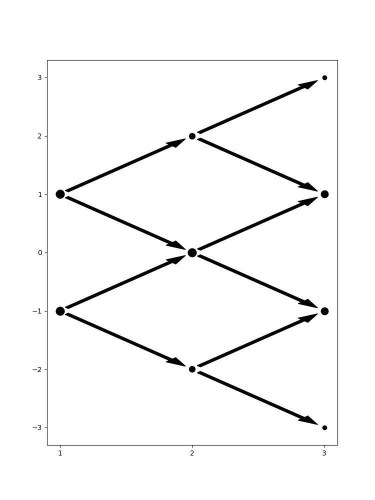
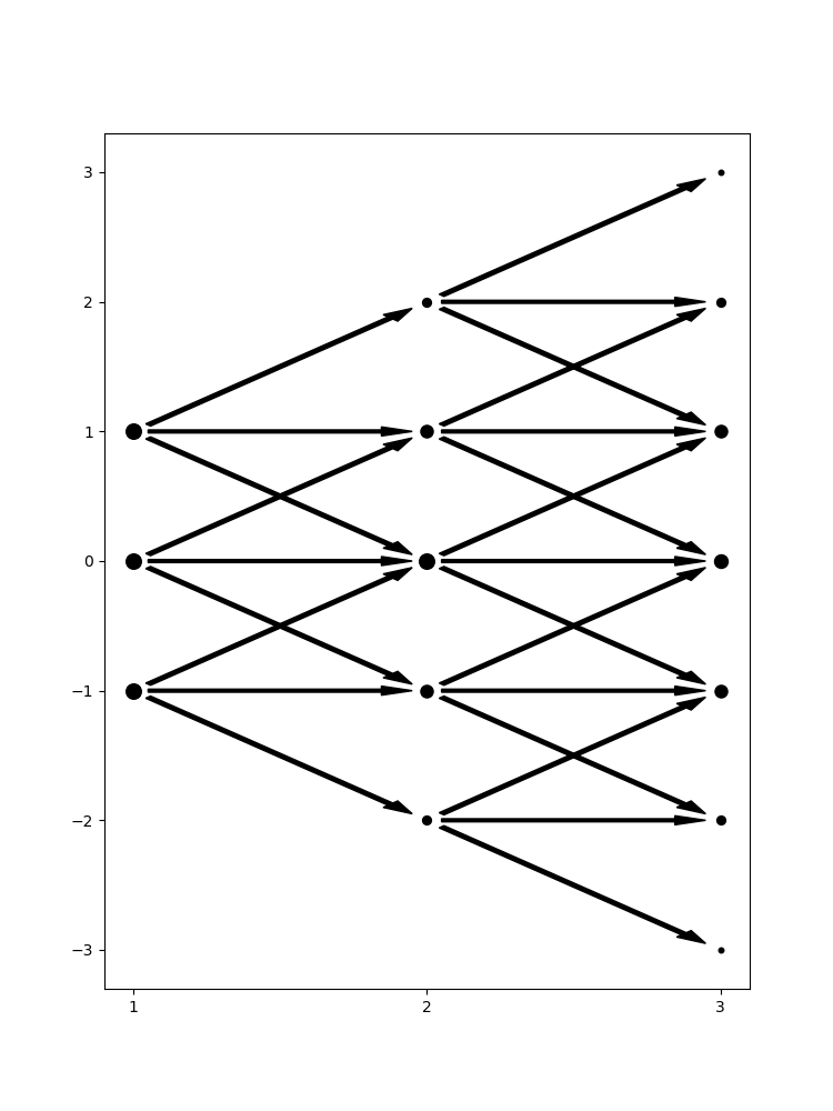
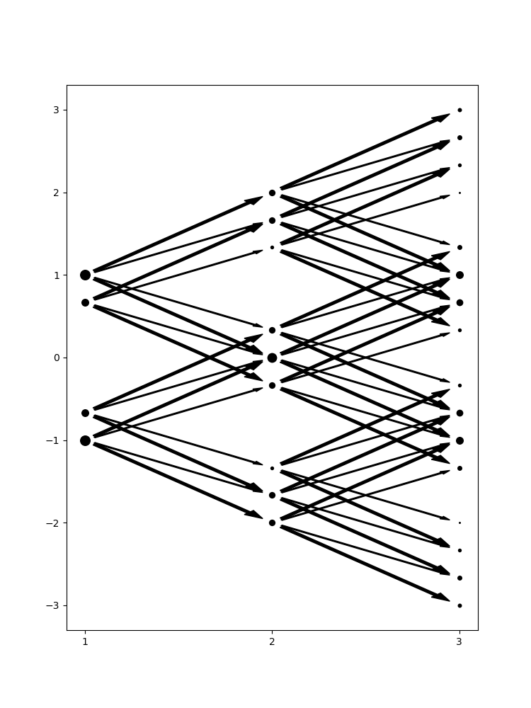
Figure 1: The binomial model $\mu$ on the left, the trinomial model $\nu$ in the middle, and the interpolating measure $\kappa_{1/3}$ under $W_{G,2}$ on the right as given by Corollary 4.10 using the euclidean distance on $\mathbb{R}^{3}$ as the underlying metric.

Next, we study an example where standard Wasserstein interpolation between two $G$-compatible measures leads to distributions that are far from $G$-compatible.

Example 4.12.

Consider the same setup as in Example 4.11. Denote by $\mu$ the distribution of the random walk $(X_{1},X_{2},X_{3})$ given by $X_{i}=\sum_{j=1}^{i}\xi_{j}$ for i.i.d. innovations $\xi_{j}$ with distribution $\mathbb{P}[\xi_{j}=\pm 1]=1/2$ and $\nu$ the distribution of $(Y_{1},Y_{2},Y_{3})$ given by $Y_{i}=\sum_{j=1}^{i}\eta_{j}$ for i.i.d. innovations $\eta_{j}$ with distribution $\mathbb{P}[\eta_{j}=-1,0,1]=1/3$. The first two pictures in Figure 1 show all possible trajectories of $X=(X_{1},X_{2},X_{3})$ and $Y=(Y_{1},Y_{2},Y_{3})$, respectively.

For the standard Wasserstein distance $W_{2}(\mu,\nu)$, a numerically obtained optimal coupling $\pi$ can be seen to satisfy

$$\pi\big{(}(X_{3},Y_{3})=(1,0)\mid(X_{1},Y_{1})=(-1,0),(X_{2},Y_{2})=(0,0)\big{)}$$

$$<\pi\big{(}(X_{3},Y_{3})=(1,0)\mid(X_{1},Y_{1})=(1,0),(X_{2},Y_{2})=(0,0)\big{)},$$

showing that $(X_{i},Y_{i})_{i=1,2,3}$ is not Markovian under $\pi$. It follows that, for all but finitely many $\lambda\in[0,1]$, the resulting interpolations $\kappa_{\lambda}$ under this coupling $\pi$ are also not Markovian.

On the other hand, using a $W_{G,p}$ interpolation as given by Corollary 4.10, the resulting interpolating measures $\kappa_{\lambda}$ are Markovian for all but finitely many $\lambda\in[0,1]$. The last picture in Figure 1 shows an illustration of the numerically computed causal interpolation $\kappa_{1/3}$.

Appendix A Stability of conditional independence

Lemma A.1.

Let $\mathcal{S},\mathcal{W},\mathcal{Z}$ be measurable spaces and $S,W,Z$ the projections from $\mathcal{S}\times\mathcal{W}\times\mathcal{Z}$ to $\mathcal{S}$, $\mathcal{W}$, $\mathcal{Z}$, respectively. Denote by $\mathcal{P}(\mathcal{S}\times\mathcal{W}\times\mathcal{Z})$ the collection of all probability measures on $\mathcal{S}\times\mathcal{W}\times\mathcal{Z}$ equipped with the product $\sigma$-algebra. Then the set

$$\{\pi\in\mathcal{P}(\mathcal{S}\times\mathcal{W}\times\mathcal{Z}):S{\perp\!\!\!\perp}_{Z}W\mbox{ with respect to }\pi\}$$ (A.1)

is closed under convergence in total variation.

Proof.

Let $(\pi^{k})_{k\in\mathbb{N}}$ be a sequence in (A.1) converging to a measure $\pi\in\mathcal{P}(\mathcal{S}\times\mathcal{W}\times\mathcal{Z})$ in total variation. By (3.2), one has

$$\pi^{k}[A\times\mathcal{W}\times\mathcal{Z}\mid W,Z]=\pi^{k}[A\times\mathcal{W}\times\mathcal{Z}\mid Z]\quad\mbox{$\pi^{k}$-a.s.}$$ (A.2)

for every measurable subset $A\subseteq\mathcal{S}$ and all $k\in\mathbb{N}$. Let us denote

$$H_{k}=\pi^{k}[A\times\mathcal{W}\times\mathcal{Z}\mid Z]\quad\mbox{and}\quad H=\pi[A\times\mathcal{W}\times\mathcal{Z}\mid Z].$$

If $\mathbb{E}^{k}$ denotes expectation with respect to $\pi^{k}$ and $\mathbb{E}$ expectation with respect to $\pi$, one has

$$\left|\mathbb{E}^{k}U-\mathbb{E}\,U\right|=\left|\int_{0}^{1}\left(\pi^{k}[U>u]-\pi[U>u]\right)du\right|\leq\int_{0}^{1}\left|\pi^{k}[U>u]-\pi[U>u]\right|du$$

for all random variables $U\colon\mathcal{S}\times\mathcal{W}\times\mathcal{Z}\to[0,1]$, which shows that for every $\varepsilon>0$, there exists a $k_{0}\in\mathbb{N}$ such that

$$\left|\mathbb{E}^{k}U-\mathbb{E}\,U\right|\leq\varepsilon\quad\mbox{for every }k\geq k_{0}\mbox{ and all such $U$.}$$

In particular,

$$\left|\mathbb{E}^{k}(1_{A\times\mathcal{W}\times\mathcal{Z}}-H)^{2}-\mathbb{E}\,(1_{A\times\mathcal{W}\times\mathcal{Z}}-H)^{2}\right|\leq\varepsilon$$

and

$$\left|\mathbb{E}^{k}(1_{A\times\mathcal{W}\times\mathcal{Z}}-H_{k})^{2}-\mathbb{E}\,(1_{A\times\mathcal{W}\times\mathcal{Z}}-H_{k})^{2}\right|\leq\varepsilon$$

for all $k\geq k_{0}$. Moreover, since the $H_{k}$ can be viewed as $L^{2}$-projections of $1_{A\times\mathcal{W}\times\mathcal{Z}}$ on the space of square-integrable $Z$-measurable random variables, one has

$$\mathbb{E}^{k}(1_{A\times\mathcal{W}\times\mathcal{Z}}-H_{k})^{2}\leq\mathbb{E}^{k}(1_{A\times\mathcal{W}\times\mathcal{Z}}-H)^{2}.$$

Together with Pythagoras’s theorem this gives

$$\mathbb{E}(H_{k}-H)^{2} = \mathbb{E}(1_{A\times\mathcal{W}\times\mathcal{Z}}-H_{k})^{2}-\mathbb{E}(1_{A\times\mathcal{W}\times\mathcal{Z}}-H)^{2}$$

$$\leq \mathbb{E}^{k}(1_{A\times\mathcal{W}\times\mathcal{Z}}-H_{k})^{2}+\varepsilon-\mathbb{E}(1_{A\times\mathcal{W}\times\mathcal{Z}}-H)^{2}$$

$$\leq \mathbb{E}^{k}(1_{A\times\mathcal{W}\times\mathcal{Z}}-H)^{2}+\varepsilon-\mathbb{E}(1_{A\times\mathcal{W}\times\mathcal{Z}}-H)^{2}$$

$$\leq \mathbb{E}(1_{A\times\mathcal{W}\times\mathcal{Z}}-H)^{2}+2\varepsilon-\mathbb{E}(1_{A\times\mathcal{W}\times\mathcal{Z}}-H)^{2}=2\varepsilon\quad\mbox{for all }k\geq k_{0},$$

showing that $H_{k}\to H$ in $L^{2}(\pi)$. Analogously, one obtains that $\pi^{k}[A\times\mathcal{W}\times\mathcal{Z}\mid W,Z]$ converges to $\pi[A\times\mathcal{W}\times\mathcal{Z}\mid W,Z]$ in $L^{2}(\pi)$. So, equation (A.2) is stable under convergence in total variation, which proves the lemma. ∎

Appendix B Counterexample to the triangle inequality

In this section, we provide an example showing that in general, $W_{G,1}$ does not satisfy the triangle inequality. We consider the Markovian graph $G=(V,E)$ with vertices $V=\{1,2,3\}$ and edges $\{(1,2),(2,3)\}$ and choose $\mathcal{X}=\mathcal{X}_{1}\times\mathcal{X}_{2}\times\mathcal{X}_{3}$, where $\mathcal{X}_{1}$, $\mathcal{X}_{2}$, $\mathcal{X}_{3}$ are all equal to the same abstract discrete Polish space $\left\{x_{1},x_{2},x_{3},x_{4}\right\}$. Note that the following three measures are all Markovian:

$$\mu =\frac{1}{4}\left(\delta_{(x_{1},x_{1},x_{1})}+\delta_{(x_{1},x_{1},x_{2})}+\delta_{(x_{2},x_{1},x_{1})}+\delta_{(x_{2},x_{1},x_{2})}\right)$$

$$\nu =\frac{1}{4}\left(\delta_{(x_{1},x_{2},x_{1})}+\delta_{(x_{1},x_{2},x_{2})}+\delta_{(x_{2},x_{3},x_{1})}+\delta_{(x_{2},x_{3},x_{2})}\right)$$

$$\eta =\frac{1}{4}\left(\delta_{(x_{3},x_{4},x_{3})}+\delta_{(x_{3},x_{4},x_{4})}+\delta_{(x_{4},x_{4},x_{3})}+\delta_{(x_{4},x_{4},x_{4})}\right).$$

We specify the distances between the 12 sequences $(x_{1},x_{1},x_{1}),(x_{1},x_{1},x_{2}),\dots$ used to define the measures $\mu,\nu,\eta$ with the following $12\times 12$ matrix $M$:

$$\setcounter{MaxMatrixCols}{12}\begin{bmatrix}0&0.53&1.08&1.33&1.29&0.78&0.64&0.44&1.15&1.3&1.92&1.38\\ 0.53&0&0.7&1.05&1.18&0.91&0.11&0.97&1.1&1.83&1.9&1.91\\ 1.08&0.7&0&0.98&1.11&0.49&0.59&0.64&0.86&1.88&1.82&1.58\\ 1.33&1.05&0.98&0&0.13&1.15&0.94&0.98&1.52&1.25&1.87&1.92\\ 1.29&1.18&1.11&0.13&0&1.02&1.07&0.85&1.39&1.38&2&1.79\\ 0.78&0.91&0.49&1.15&1.02&0&1.02&1.13&0.37&1.74&1.77&1.22\\ 0.64&0.11&0.59&0.94&1.07&1.02&0&1.08&1.21&1.94&1.79&2.02\\ 0.44&0.97&0.64&0.98&0.85&1.13&1.08&0&1.5&1.24&1.86&0.94\\ 1.15&1.1&0.86&1.52&1.39&0.37&1.21&1.5&0&1.37&1.4&0.85\\ 1.3&1.83&1.88&1.25&1.38&1.74&1.94&1.24&1.37&0&0.62&1.2\\ 1.92&1.9&1.82&1.87&2&1.77&1.79&1.86&1.4&0.62&0&1.69\\ 1.38&1.91&1.58&1.92&1.79&1.22&2.02&0.94&0.85&1.2&1.69&0\end{bmatrix}.$$

That is, $M_{1,2}$ is the distance between $(x_{1},x_{1},x_{1})$ and $(x_{1},x_{1},x_{2})$, $M_{1,3}$ is the distance between $(x_{1},x_{1},x_{1})$ and $(x_{2},x_{1},x_{1})$ and so on. We obtained $M$ by simulating symmetric matrices with zeros on the diagonal and positive entries off the diagonal and iteratively updating the entries as long as the triangle inequality was violated. More precisely, we started with a symmetric random matrix $M^{0}$ with zeros on the diagonal and positive off-diagonal entries. Then we iteratively set

$$M^{k}_{i,j}=\min\{M^{k-1}_{i,j},M^{k-1}_{i,1}+M^{k-1}_{1,j},M^{k-1}_{i,2}+M^{k-1}_{2,j},\dots,M^{k-1}_{i,12}+M^{k-1}_{12,j}\}$$

until $M^{k}=M^{k-1}$. This guarantees that $M$ defines a metric on $(x_{1},x_{1},x_{1}),(x_{1},x_{1},x_{2})\dots$ From there it can be extended to a metric on $\mathcal{X}$ by Fréchet embedding. Finally, we used Gurobi [28] to compute $W_{G,1}(\mu,\nu)=0.585$, $W_{G,1}(\nu,\eta)=2.24$ and $W_{G,1}(\mu,\eta)=2.925$, showing that

$$W_{G,1}(\mu,\eta)>W_{G,1}(\mu,\nu)+W_{G,1}(\nu,\eta).$$

References

- Acciaio et al. [2021] Beatrice Acciaio, Julio Backhoff-Veraguas, and Junchao Jia. Cournot–Nash equilibrium and optimal transport in a dynamic setting. SIAM Journal on Control and Optimization, 59(3):2273–2300, 2021.
- Agueh and Carlier [2011] Martial Agueh and Guillaume Carlier. Barycenters in the Wasserstein space. SIAM Journal on Mathematical Analysis, 43(2):904–924, 2011.
- Aldous [1981] David Aldous. Weak convergence and the general theory of processes. Incomplete Draft, 1981. URL https://www.stat.berkeley.edu/~aldous/Papers/weak-gtp.pdf.
- Arjovsky et al. [2017] Martin Arjovsky, Soumith Chintala, and Léon Bottou. Wasserstein generative adversarial networks. In International Conference on Machine Learning, pages 214–223. PMLR, 2017.
- Backhoff-Veraguas and Pammer [2022] Julio Backhoff-Veraguas and Gudmund Pammer. Stability of martingale optimal transport and weak optimal transport. The Annals of Applied Probability, 32(1):721–752, 2022.
- Backhoff-Veraguas et al. [2017] Julio Backhoff-Veraguas, Mathias Beiglböck, Yiqing Lin, and Anastasiia Zalashko. Causal transport in discrete time and applications. SIAM Journal on Optimization, 27(4):2528–2562, 2017.
- Backhoff-Veraguas et al. [2020] Julio Backhoff-Veraguas, Daniel Bartl, Mathias Beiglböck, and Manu Eder. All adapted topologies are equal. Probability Theory and Related Fields, 178(3):1125–1172, 2020.
- Bartl et al. [2021] Daniel Bartl, Mathias Beiglböck, and Gudmund Pammer. The Wasserstein space of stochastic processes. arXiv Preprint 2104.14245, 2021.
- Beiglböck and Juillet [2016] Mathias Beiglböck and Nicolas Juillet. On a problem of optimal transport under marginal martingale constraints. The Annals of Probability, 44(1):42–106, 2016.
- Blanchet and Murthy [2019] Jose Blanchet and Karthyek Murthy. Quantifying distributional model risk via optimal transport. Mathematics of Operations Research, 44(2):565–600, 2019.
- Bongers et al. [2021] Stephan Bongers, Patrick Forré, Jonas Peters, and Joris M Mooij. Foundations of structural causal models with cycles and latent variables. The Annals of Statistics, 49(5):2885–2915, 2021.
- Bonneel and Coeurjolly [2019] Nicolas Bonneel and David Coeurjolly. Spot: sliced partial optimal transport. ACM Transactions on Graphics (TOG), 38(4):1–13, 2019.
- Bourbaki [1966] Nicolas Bourbaki. Elements of Mathematics: General Topology, Part 2. Actualités Scientifiques et Industrielles. Hermann, 1966. URL https://books.google.de/books?id=y1wnAQAAIAAJ.
- Cheridito et al. [2017] Patrick Cheridito, Michael Kupper, and Ludovic Tangpi. Duality formulas for robust pricing and hedging in discrete time. SIAM Journal on Financial Mathematics, 8(1):738–765, 2017.
- Cheridito et al. [2021] Patrick Cheridito, Matti Kiskii, David Prömel, and Mete Soner. Martingale optimal transport duality. Mathematische Annalen, 379:1685–1712, 2021.
- Chiappori et al. [2010] Pierre-André Chiappori, Robert J McCann, and Lars P Nesheim. Hedonic price equilibria, stable matching, and optimal transport: equivalence, topology, and uniqueness. Economic Theory, pages 317–354, 2010.
- Chizat et al. [2018] Lenaic Chizat, Gabriel Peyré, Bernhard Schmitzer, and François-Xavier Vialard. Unbalanced optimal transport: Dynamic and Kantorovich formulations. Journal of Functional Analysis, 274(11):3090–3123, 2018.
- Cuturi [2013] Marco Cuturi. Sinkhorn distances: lightspeed computation of optimal transport. Advances in Neural Information Processing Systems, 26, 2013.
- Cuturi and Doucet [2014] Marco Cuturi and Arnaud Doucet. Fast computation of Wasserstein barycenters. In International Conference on Machine Learning, pages 685–693. PMLR, 2014.
- De Gennaro Aquino and Eckstein [2020] Luca De Gennaro Aquino and Stephan Eckstein. Minmax methods for optimal transport and beyond: Regularization, approximation and numerics. Advances in Neural Information Processing Systems, 33:13818–13830, 2020.
- De Lara et al. [2021] Lucas De Lara, Alberto González-Sanz, Nicholas Asher, and Jean-Michel Loubes. Transport-based counterfactual models. arXiv Preprint 2108.13025, 2021.
- De Philippis and Figalli [2014] Guido De Philippis and Alessio Figalli. The Monge–Ampère equation and its link to optimal transportation. Bulletin of the American Mathematical Society, 51(4):527–580, 2014.
- Embrechts et al. [2013] Paul Embrechts, Giovanni Puccetti, and Ludger Rüschendorf. Model uncertainty and VaR aggregation. Journal of Banking & Finance, 37(8):2750–2764, 2013.
- Figalli et al. [2010] Alessio Figalli, Francesco Maggi, and Aldo Pratelli. A mass transportation approach to quantitative isoperimetric inequalities. Inventiones Mathematicae, 182(1):167–211, 2010.
- Fournier and Guillin [2015] Nicolas Fournier and Arnaud Guillin. On the rate of convergence in Wasserstein distance of the empirical measure. Probability Theory and Related Fields, 162(3):707–738, 2015.
- Galichon [2018] Alfred Galichon. Optimal Transport Methods in Economics. Princeton University Press, 2018.
- Ghosal and Sen [2022] Promit Ghosal and Bodhisattva Sen. Multivariate ranks and quantiles using optimal transport: consistency, rates and nonparametric testing. The Annals of Statistics, 50(2):1012–1037, 2022.
- Gurobi Optimization, LLC [2022] Gurobi Optimization, LLC. Gurobi Optimizer Reference Manual, 2022. URL https://www.gurobi.com.
- Hellwig [1996] Martin Hellwig. Sequential decisions under uncertainty and the maximum theorem. Journal of Mathematical Economics, 25(4):443–464, 1996.
- Holland [1986] Paul W Holland. Statistics and causal inference. Journal of the American Statistical Association, 81(396):945–960, 1986.
- Huang et al. [2022] Yiyan Huang, Cheuk Hang Leung, Qi Wu, Xing Yan, Shumin Ma, Zhiri Yuan, Dongdong Wang, and Zhixiang Huang. Robust causal learning for the estimation of average treatment effects. In 2022 International Joint Conference on Neural Networks (IJCNN 2022). IEEE, 2022.
- [32] Olav Kallenberg. Foundations of Modern Probability, 3rd Edition. Springer. doi: https://doi.org/10.1007/978-3-030-61871-1.
- Kantorovich [1939] Leonid V Kantorovich. Mathematical methods of organizing and planning production. Management Science, 6(4):366–422, 1939.
- Kantorovich [1942] Leonid V Kantorovich. On the translocation of masses. In Dokl. Akad. Nauk. USSR (NS), volume 37, pages 199–201, 1942.
- Kocaoglu et al. [2018] Murat Kocaoglu, Christopher Snyder, Alexandros G Dimakis, and Sriram Vishwanath. Causalgan: learning causal implicit generative models with adversarial rraining. In International Conference on Learning Representations, 2018.
- Korman and McCann [2015] Jonathan Korman and Robert McCann. Optimal transportation with capacity constraints. Transactions of the American Mathematical Society, 367(3):1501–1521, 2015.
- Lassalle [2018] Rémi Lassalle. Causal transport plans and their Monge–Kantorovich problems. Stochastic Analysis and Applications, 36(3):452–484, 2018.
- Lauritzen [1996] Steffen L Lauritzen. Graphical Models, volume 17. Clarendon Press, 1996.
- Li and Lin [2021] Jia Li and Lin Lin. Optimal transport with relaxed marginal constraints. IEEE Access, 9:58142–58160, 2021.
- Lorenz et al. [2021] Dirk A Lorenz, Paul Manns, and Christian Meyer. Quadratically regularized optimal transport. Applied Mathematics & Optimization, 83(3):1919–1949, 2021.
- Mémoli [2011] Facundo Mémoli. Gromov–Wasserstein distances and the metric approach to object matching. Foundations of Computational Mathematics, 11(4):417–487, 2011.
- Mohajerin Esfahani and Kuhn [2018] Peyman Mohajerin Esfahani and Daniel Kuhn. Data-driven distributionally robust optimization using the Wasserstein metric: Performance guarantees and tractable reformulations. Mathematical Programming, 171(1-2):115–166, 2018.
- Monge [1781] Gaspard Monge. Mémoire sur la théorie des déblais et des remblais. Mem. Math. Phys. Acad. Royale Sci., pages 666–704, 1781.
- Niles-Weed and Berthet [2022] Jonathan Niles-Weed and Quentin Berthet. Minimax estimation of smooth densities in Wasserstein distance. The Annals of Statistics, 50(3):1519–1540, 2022.
- Nutz and Wang [2022] Marcel Nutz and Ruodu Wang. The directional optimal transport. The Annals of Applied Probability, 32(2):1400–1420, 2022.
- Pammer [2022] Gudmund Pammer. A note on the adapted weak topology in discrete time. arXiv Preprint 2205.00989, 2022.
- Pass [2015] Brendan Pass. Multi-marginal optimal transport: theory and applications. ESAIM: Mathematical Modelling and Numerical Analysis, 49(6):1771–1790, 2015.
- Pearl [2009] Judea Pearl. Causality. Cambridge university press, 2009.
- Peters et al. [2016] Jonas Peters, Peter Bühlmann, and Nicolai Meinshausen. Causal inference by using invariant prediction: identification and confidence intervals. Journal of the Royal Statistical Society: Series B (Statistical Methodology), 78(5):947–1012, 2016.
- Peyré and Cuturi [2019] Gabriel Peyré and Marco Cuturi. Computational Optimal Transport: With Applications to Data Science. Now Publishers and Trends, 2019.
- Pflug and Pichler [2012] Georg Pflug and Alois Pichler. A distance for multistage stochastic optimization models. SIAM Journal on Optimization, 22(1):1–23, 2012.
- Pflug and Pichler [2015] Georg Pflug and Alois Pichler. Dynamic generation of scenario trees. Computational Optimization and Applications, 62(3):641–668, 2015.
- Pflug et al. [2012] Georg Ch Pflug, Alois Pichler, and David Wozabal. The 1/n investment strategy is optimal under high model ambiguity. Journal of Banking & Finance, 36(2):410–417, 2012.
- Plecko and Meinshausen [2020] Drago Plecko and Nicolai Meinshausen. Fair data adaptation with quantile preservation. Journal of Machine Learning Research, 21(242):1–44, 2020.
- [55] Svetlozar T Rachev. The monge–kantorovich mass transference prob- lem and its stochastic applications.
- Rachev and Rüschendorf [1998] Svetlozar T Rachev and Ludger Rüschendorf. Mass Transportation Problems. Vol. I Theory, Vol. II Applications. Springer Verlag, Berlin, 1998.
- Sävje et al. [2021] Fredrik Sävje, Peter Aronow, and Michael Hudgens. Average treatment effects in the presence of unknown interference. Annals of Statistics, 49(2):673, 2021.
- Schölkopf [2022] Bernhard Schölkopf. Causality for machine learning. In Probabilistic and Causal Inference: The Works of Judea Pearl, pages 765–804. 2022.
- Séjourné et al. [2022] Thibault Séjourné, Gabriel Peyré, and François-Xavier Vialard. Unbalanced optimal transport, from theory to numerics. arxiv Preprint 2211.08775, 2022.
- [60] Bharath K Sriperumbudur, Kenji Fukumizu, Arthur Gretton, and Sch/"olkopf. On the empirical estimation of integral probability metrics.
- Sudakov [1976] V. N. Sudakov. Geometric problems of the theory of infinite-dimensional probability distributions. Trudy Mat. Inst. Steklov, 141:3–191, 1976.
- Titouan et al. [2020] Vayer Titouan, Ievgen Redko, Rémi Flamary, and Nicolas Courty. Co-optimal transport. Advances in Neural Information Processing Systems, 33:17559–17570, 2020.
- Tran et al. [2021] Quang Huy Tran, Hicham Janati, Ievgen Redko, Flamary Rémi, and Nicolas Courty. Factored couplings in multi-marginal optimal transport via difference of convex programming. NeurIPS 2021 Optimal Transport and Machine Learning Workshop (OTML), 2021.
- Vallender [1974] Sergey S Vallender. Calculation of the Wasserstein distance between probability distributions on the line. Theory of Probability & Its Applications, 18(4):784–786, 1974.
- Villani [2009] Cédric Villani. Optimal Transport: Old and New, volume 338. Springer, 2009.
- Wasserstein [1969] Leonid Nisonovich Wasserstein. Markov processes over denumerable products of spaces, describing large systems of automata. Problemy Peredachi Informatsii, 5(3):64–72, 1969.
- Xu and Acciaio [2021] Tianlin Xu and Beatrice Acciaio. Quantized conditional cot-gan for video prediction. arXiv Preprint 2106.05658, 2021.
- Xu et al. [2020] Tianlin Xu, Li Kevin Wenliang, Michael Munn, and Beatrice Acciaio. Cot-gan: generating sequential data via causal optimal transport. Advances in Neural Information Processing Systems, 33:8798–8809, 2020.
- [69] I Yang. A convex optimization approach to distributionally robust Markov decision processes with Wasserstein distance. IEEE Control Systems Letters.