Online Learning for the Random Feature Model in the Student-Teacher Framework

Abstract

Deep neural networks are widely used prediction algorithms whose performance often improves as the number of weights increases, leading to over-parametrization. We consider a two-layered neural network whose first layer is frozen while the last layer is trainable, known as the random feature model. We study over-parametrization in the context of a student-teacher framework by deriving a set of differential equations for the learning dynamics. For any finite ratio of hidden layer size and input dimension, the student cannot generalize perfectly, and we compute the non-zero asymptotic generalization error. Only when the student’s hidden layer size is exponentially larger than the input dimension, an approach to perfect generalization is possible.

1 Introduction

Deep neural networks (DNNs) have a wide range of applications. Besides the most well-known areas, such as image classification and speech recognition, there are numerous applications within physics (LeCun et al., 2015; Goodfellow et al., 2016; Krizhevsky et al., 2012; Silver et al., 2017; Carleo et al., 2019). Often, DNN performance improves as the number of weights increases, generating networks that have far more free parameters available than training data, a regime which reveals exciting properties (Zhang et al., 2021; Theunissen et al., 2020; Canziani et al., 2017; Novak et al., 2019; Neyshabur et al., 2019; Bartlett, 1998). When initializing the weights randomly and independently with zero mean and a variance inversely proportional to the network width, the network’s output in the infinite width limit is described by a Gaussian process with an analytically accessible covariance matrix (Neal, 1996; Lee et al., 2018; Novak et al., 2019; de G. Matthews et al., 2018; Williams, 1996). However, the evolution of network weights during training and the corresponding improvement of prediction performance are not fully understood yet.

In the ultra-wide limit for which the neural network size tends to infinity, recent studies have revealed that over-parametrized neural networks trained by stochastic gradient descent can be described by two different limits, depending on the scaling of the output layer (Geiger et al., 2020). In order to realize the so-called neural tangent kernel (NTK) limit, the network output is scaled by the square root of the network width. In this limit, the stochastic gradient descent changes the weights of the network very slowly, resulting in weigth dynamics equivalent to that of a linearized network, and the evolution of network predictions during the learning process is described by the so-called neural tangent kernel (Jacot et al., 2018). This limit is also known as the lazy training regime, for which the network weights stay in the vicinity of their initial values during the learning process, and for which the NTK does not change during training in the ultra-wide limit (Chizat et al., 2019).

Here, we study a student-teacher secanario in the NTK limit, which allows us to analyze the generalization performance and convergence properties of wide over-parametrized neural networks (Arora et al., 2019a). However, it is not entirely clear whether the NTK framework can fully explain the performance of DNNs. Using certain data sets, the autors of (Arora et al., 2019b) showed that the NTK limit achieves good generalization performance, and in (Lee et al., 2019) it was found found that the prediction of the NTK limit is in correspondence with certain over-parametrized and in-practice used neural networks. In contrast, (Chizat et al., 2019; Ghorbani et al., 2019; Yehudai & Shamir, 2019) highlighted that the NTK limit cannot explain the generalization performance of over-parametrized neural networks since a performance gap was revealed. This performance gap was recently confirmed by (Samarin et al., 2022) empirically for finite and practically relevant networks. In this work, we want to further quantify this performance gap analytically and analyze under which circumstances a DNN in the NTK limit can be expected to perform well.
Throughout this paper, we consider two-layer neural networks in the lazy training regime, resulting in a linear learning dynamics described by the NTK (Rahimi & Recht, 2008). In order to study the behavior of neural networks in the NTK limit qualitatively, we freeze the first layer weights mimicking their laziness and train only the hidden-to-output neurons. Such a network architecture is known as the random feature model (RFM) (Rahimi & Recht, 2007), where the feature map is equivalent to the activations of the hidden neurons. The RFM corresponds to the part of a fully linearized two-layer neural network where one linearizes the network’s output for hidden-to-output weights only and neglects the linearization with respect to input-to-hidden weights. However, on a qualitative level the results for a RFM and the full NTK limit may be similar since freezing the input-to-hidden neurons may not affect the predictors class .
In this paper, we use techniques from statistical mechanics to analyze the learning dynamics of highly over-aprametrized random feature models with a large hidden and input layer. The network is trained by one-pass stochastic gradient descent, defining the system’s dynamics. In order to express over-parametrization, we use the student-teacher framework for which the student is trained by the outputs of a teacher (Gardner & Derrida, 1989). In this setup, the number of student hidden nodes $K$ is larger or equal to the number of teacher hidden nodes $M$. In such a case, the student is potentially more powerful than the teacher and can express more complex functions. Moreover, we are interested in the influence of the ratio of hidden-layer width $K$ to input-layer size $N$ on the student performance. Since over-parametrized networks have many degrees of freedom, statistical mechanics forms an important branch of theory deriving macroscopic properties from the interaction of network weights (Hertz et al., 1991; Watkin et al., 1993; Saad, 2000; Engel & Van den Broeck, 2001; Bahri et al., 2020). It was successfully used to study the perceptron (Gardner, 1988; Györgyi & Tishby, 1990; Seung et al., 1992), two-layer neural networks (Opper, 1994; Riegler & Biehl, 1995; Goldt et al., 2019; Schwarze & Hertz, 1993; Biehl & Schwarze, 1995; Saad & Solla, 1995b, a; Biehl et al., 1996, 1998; Oostwal et al., 2021; Richert et al., 2022), and more general (deep) architectures (Naveh et al., 2021; Li & Sompolinsky, 2021; Cohen et al., 2021). Other interesting investigations deal with the influence of the input structure on the learning process (Goldt et al., 2020; Yoshida & Okada, 2020).

2 Related work

Based on the bias-variance tradeoff, traditional learning theories suggest that over-parametrized neural networks should generalize poorly as they have more regression parameters than avaiable input examples (Geman et al., 1992). However, recent studies have shown that this tradeoff must be extend for ultra-wide neural networks leading to a double descent curve (Belkin et al., 2019). For the RFM, different analytical studies derived the test error’s double descent behavior in the student-teacher framework indicating the accessibility of interesting deep learning phenomena by investigating this model (Advani et al., 2020; D’Ascoli et al., 2020; Mei & Montanari, 2022; Hastie et al., 2022).

Related work has shown that the RFM cannot predict the output of a ReLU perceptron, except the hidden layer size $K$ increases exponentially fast with the input dimension $N$ (Yehudai & Shamir, 2019). We verify this result for an error activation function by actually computing the asymptotic generalization error. Further related studies considered the random feature model for quadratic activation and output functions in the high-dimensional regime $K,N\rightarrow\infty$, $K/N\rightarrow\tau\in\left(0,\infty\right)$ trained by one-pass stochastic gradient descent (Ghorbani et al., 2019). These works demonstrated the existence of a gap between the performance of the RFM compared to fully-trained over-parametrized neural networks. (Mei et al., 2022) provide a general expresssion for the generalization error of random feature models, relating it to the projection of the target function on the span of kernel eigenfunctions which are not learned in the regime of $K/N$-finite. Here, we provide an explicit expression for the $K/N$ dependence of the generalization error for the case of the error and ReLU activation function. Furthermore, the network performance is highly controlled by the initialization of the weights and becomes optimal only in the case for which the random features are perfectly aligned with those of the teacher. For $K\propto N$ (Ghorbani et al., 2021) have shown that the student is just able to learn linear teachers. This regime lies in our focus and justifies the linearization of the random feature correlation matrices introduced in Chapter 5. We further extend investigations by introducing a set of ordinary differential equations for the learning dynamics of a student with infinitely large input and hidden layer size trained by a teacher with a ReLU or error activation function. We find that the generalization error converges to a finite plateau whenever the ratio of the input-to-hidden layer size is finite and compute the plateau heights for different activation functions rather than providing error bounds.

3 Setup

For our setup, the student and teacher receive input samples $\bm{\xi}^{\mu}\in\mathbb{R}^{N}$ presented once and in a sequential order where each component is generated by the normal distribution $\xi_{i}^{\mu}\in\mathcal{N}\left(0,1\right)$ with $\mu\in\{1,...,p\}$. The student has $K$ hidden neurons and the connection between the input layer with the $i$-th hidden node is expressed by the student vectors $\bm{J}_{i}\in\mathbb{R}^{N}$. The outputs of the hidden nodes are given by a continuous activation function $g$. The overall output of the network is a linear combination of the outputs of the hidden units

$$\sigma\left(\bm{J},\bm{\xi}\right)=\sum^{K}_{i}c_{i}g\left(x_{i}\right),$$ (1)

with $c_{i}$ are the hidden-to-output weights and the pre-activations of the student are defined by $x_{i}=\frac{\bm{J}_{i}\cdot\bm{\xi}}{\sqrt{N}}$. Note that the rescaling factor $\frac{1}{\sqrt{N}}$ guarantees pre-activations of $O\left(1\right)$. The teacher has $M$ hidden neurons characterized by the teacher vectors $\bm{B}_{n}\in\mathbb{R}^{N}$ and provides the output $\zeta(\bm{B},\bm{\xi})=\frac{1}{\sqrt{M}}\sum_{n=1}^{M}g\left(y_{n}\right)$ with $y_{n}=\frac{\bm{B}_{n}\cdot\bm{\xi}}{\sqrt{N}}$ as the pre-activations of the teacher. However, it turns out that increasing the teacher size $M$ does not influence the learning process qualitatively and we therefore consider a teacher perceptron with $M=1$.

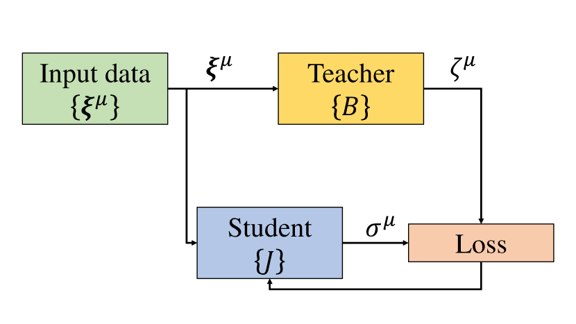
Figure 1: Schematic illustration of the learning problem. An environment generates input data $\{\bm{\xi}^{\mu}\}$ according to a probability distribution. The student and teacher receive this data. Both release their outputs according to their parameter sets $\{J\}$ and $\{B\}$, respectively. The loss quantifies the dissimilarity between the student output $\sigma^{\mu}$ and teacher output $\zeta^{\mu}$. It sends feedback to the student for the adaptation of the parameters $\{J\}$. The overall goal is to minimize the loss during the learning process.

We choose the student and teacher vectors independently from the uniform distribution over the $N$ sphere and initialize the output weights of the student by the normal distribution with $c_{i}\in\mathcal{N}\left(0,\frac{1}{K}\right)$. In practice, we initialize the components of the student and teacher vectors by the normal distribution $J_{i},B_{n}\in\mathcal{N}\left(0,1\right)$ and rescale them afterwards by their norm. This leads to a uniform distribution of the student and teacher vectors over the $N$ sphere with radius $\sqrt{N}$ making the student vectors to random features. As we are interested in cases for which $K>N$, the student vectors are expected to have important correlations among each other. In order to express these correlation and those of the student and teacher vectors we introduce the variables $R_{in}=\frac{\bm{J}_{i}\cdot\bm{B}_{n}}{N},Q_{ij}=\frac{\bm{J}_{i}\cdot\bm{J}_{j}}{N}$ and $T_{nm}=\frac{\bm{B}_{n}\cdot\bm{B}_{m}}{N}=\delta_{nm}$. In the case $K<N$ , one refers to these parameters as order parameters and makes the transition from a microscopic to a macroscopic description of the system. However, in our setup such an interpretation is no longer true as we are mainly interested in the case $K>N$. Previous research on initializing the student vectors over a sphere for the RFM with ReLU activations can be found in (Mei & Montanari, 2022; Yehudai & Shamir, 2019; Ghorbani et al., 2021) and for a Gaussian (mixture) initialization with quadratic activations in (Ghorbani et al., 2019).
The performance of the student with respect to the teacher is measured by the loss function $\epsilon=\frac{1}{2}\left[\zeta-\sigma\right]^{2}$ known as the mean squared error. As the distribution of the input patterns is accessible, we can take the expectation value of the loss function and define the generalization error $\epsilon_{g}=\left<\epsilon\left(c_{i},\bm{\xi}\right)\right>_{\bm{\xi}}$ depending on the correlation matrices. This makes it possible to analyze the average error of the student evaluated on unseen test data. For the error activation function, one finds for the generalization error (Saad & Solla, 1995b; Goldt et al., 2019)

$$\epsilon_{{g,}{\mathrm{erf}}}=\frac{1}{\pi}\Biggl{[} \frac{\pi}{6}+\sum_{i,j}{c_{i}c_{j}\arcsin{\left(\frac{Q_{ij}}{2}\right)}}$$

$$-2\sum_{i}{c_{i}\arcsin{\left(\frac{R_{i}}{2}\right)}}\Biggr{]}.$$ (2)

and for a ReLU activation (Oostwal et al., 2021)

$$\epsilon_{g,{\mathrm{ReLU}}}= \sum_{i,j}\frac{c_{i}c_{j}}{2}\biggl{[}\frac{Q_{ij}}{4}$$

$$+\frac{1}{2\pi}\biggl{[}\sqrt{1-Q_{ij}^{2}}+Q_{ij}\arcsin\left(Q_{ij}\right)\biggr{]}\biggr{]}$$

$$-\sum_{i}c_{i}\biggl{[}\frac{R_{i}}{4}+\frac{1}{2\pi}\biggl{[}\sqrt{1-R_{i}^{2}}+R_{i}\arcsin\left(R_{i}\right)\biggr{]}\biggr{]}$$

$$+\frac{1}{4}.$$ (3)

for the case $M=1$. Here, we have used that $\frac{1}{2}\left<\zeta(\bm{B},\bm{\xi})^{2}\right>_{\mathrm{erf}}=\frac{1}{6}$ and $\frac{1}{2}\left<\zeta(\bm{B},\bm{\xi})^{2}\right>_{\mathrm{ReLU}}=\frac{1}{4}$.

Due the special form of the mean squared loss function, the above Eqs. (2) and (3) can be subsumed in the vector-matrix-form

$$\epsilon_{g}=\frac{1}{2}\left<\zeta(\bm{B},\bm{\xi})^{2}\right>_{\xi}+\frac{1}{2}\bm{c}^{T}\tilde{\bm{Q}}\bm{c}-\bm{c}^{T}\tilde{\bm{R}}$$ (4)

with $\tilde{Q}_{ij}=\left<g\left(x_{i}\right)g\left(x_{j}\right)\right>$ and $\tilde{R}_{i}=\left<g\left(x_{i}\right)g\left(y\right)\right>$ describing the correlation between the hidden neurons. We can directly calculate the minimal generalization error by minimizing Eq. (4) with respect to the $c_{i}$, and obtain $\epsilon_{g_{\mathrm{min}}}=\frac{\left<\zeta(\bm{B},\bm{\xi})^{2}\right>_{\xi}}{2}-\frac{1}{2}\tilde{\bm{R}}^{T}\tilde{\bm{Q}}^{-1}\tilde{\bm{R}}.$, where the optimal weights are $\bm{c}_{\mathrm{min}}=\tilde{\bm{Q}}^{-1}\tilde{\bm{R}}$. Therefore, the minimum generalization error depends on the correlations of the hidden neurons and therefore on the choice of the activation function.

4 Dynamics of the System

During the learning process, we update the student weights $c_{i}$ by stochastic gradient descent after each representation of a specific input example according to

$$c_{i}^{\mu+1}-c_{i}^{\mu}=-\frac{\eta}{K}\nabla_{c_{i}}\epsilon\left(c_{i}^{\mu},\xi^{\mu}\right),$$ (5)

with $\eta$ denoting the learning rate which controls the step size in weight space. The superscript $\mu$ stands for the $\mu-$th input pattern and can be associated with a discreet time measure due to the sequential updating. Commonly, one would rescale the learning rate by $\frac{1}{N}$ in order to study the dynamics of the learning process (Engel & Van den Broeck, 2001; Riegler & Biehl, 1995; Goldt et al., 2019; Reents & Urbanczik, 1998). As in our case the first layer is fixed and just the last $K$ weights are trained, we have rescaled the learning rate by $\frac{1}{K}$ in Eq. (5) in order to guarantee small fluctuations for large size limits (Rotskoff & Vanden-Eijnden, 2022). In the ultra-wide limit $N,K,p\rightarrow\infty$ with a finite ratio $\frac{p}{K}=\alpha$, we find a Langevin equation for the student weights

$$\frac{d\bm{c}}{d\alpha}=-\eta\nabla\epsilon_{g}+\frac{\eta}{\sqrt{K}}\bm{\gamma}$$ (6)

where $\bm{\gamma}$ random is a random vector with $\left<\bm{\gamma}\right>=0$, $\left<\gamma_{i}\left(\alpha\right)\gamma_{j}\left(\alpha^{\prime}\right)\right>=\Sigma_{ij}\delta\left(\alpha-\alpha^{\prime}\right)$ and covariance matrix $\bm{\Sigma}=\left<\left(\nabla\epsilon-\nabla\epsilon_{g}\right)\left(\nabla\epsilon-\nabla\epsilon_{g}\right)^{T}\right>$.
In order to derive the Langevin equation given by Eq. (6) heuristically, we reconsider the stochastic update rule for a small ratio $\frac{\eta}{K}\rightarrow 0$ and find for the recursion relation

$$\bm{c}^{\mu+l}-\bm{c}^{\mu}\approx-\frac{\eta}{K}l\sum_{j=0}^{l-1}\frac{\nabla\epsilon\left(c^{\mu},\xi^{\mu+j}\right)}{l}.$$ (7)

Since the input examples are independent identically distributed variables which are presented only once during the whole learning process, we further assume weak correlations in the update steps. Therefore, as the sum on the right hand side is over nearly independent identically distributed variables with a finite variance, we can invoke the Central Limit Theorem (Mandt et al., 2017; Latz, 2021) and approximate the sum by

$$\sum_{j=0}^{l-1}\frac{\nabla\epsilon\left(c^{\mu+j},\xi^{\mu+j}\right)}{l}\approx\nabla\epsilon_{g}\left(c\right)+\frac{\Delta\bm{\rho}\left(c\right)}{\sqrt{l}},$$ (8)

with a random vector $\left<\Delta\bm{\rho}\right>=0$ and corresponding covariance matrix $\textrm{Cov}\left(\Delta\bm{\rho}\right)=\left<\left(\nabla\epsilon-\nabla\epsilon_{g}\right)\left(\nabla\epsilon-\nabla\epsilon_{g}\right)^{T}\right>$. Due to weak correlations in the update steps, we assume an approximately constant covariance matrix $\Sigma$ with respect to the weights $c_{i}$. As the covariance matrix is symmetric and positive-semidefinite, we can factorized it $\Sigma=\Omega\Omega^{T}$ and replace the random vector $\Delta\bm{\rho}$ by $\sqrt{\Delta\alpha}\Delta\bm{\rho}=\Omega\Delta\bm{W}$, where $\frac{l}{K}=\Delta\alpha$ is a time difference rescaled by the hidden-layer size and $\Delta\bm{W}\in\mathcal{N}\left(0,\bm{1}\right)$ is a Gaussian process. In the ultra-wide limit $K,N,l\rightarrow\infty$, Eq. (8) can be interpreted as a finite-difference equation that approximates the following continuous time stochastic differential equation

$$d\bm{c}=-\eta\nabla_{c}\epsilon_{g}d\alpha+\frac{\eta}{\sqrt{K}}\Omega d\bm{W}(\alpha)\ ,$$ (9)

with $\left<dW_{i}(\alpha)dW_{j}(\alpha)\right>=\delta_{ij}d\alpha$ as Brownian motion. The above stochastic differential equation can be recast into a Langevin form by introducing $\left<\bm{\gamma}\right>=0$, $\left<\gamma_{i}\left(\alpha\right)\gamma_{j}\left(\alpha^{\prime}\right)\right>=\Sigma_{ij}\delta\left(\alpha-\alpha^{\prime}\right)$ and $\Omega dW(\alpha)=\int_{0}^{d\alpha}d\tau\bm{\gamma}\left(\tau\right)$. More details for the Langevin equivalence of the sotchastic gradient descent can be found in (Hu et al., 2019; Mandt et al., 2017; Latz, 2021).

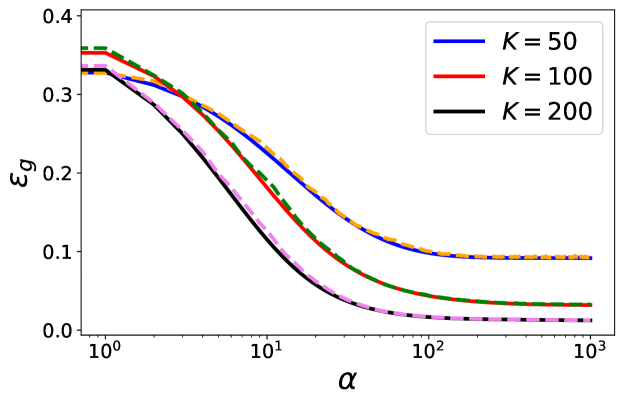
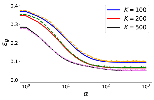
Figure 2: Generalization error as a function of $\alpha$ for an error function activation $g\left(x\right)=\mathrm{erf}\left(\frac{x}{\sqrt{2}}\right)$ (top) and ReLU activation function (bottom) for $N=100$. The numerical solutions of the differential equations (solid lines) fits well to the simulations. We use for the simulations $\eta_{\mathrm{simulation}}=\frac{0.1}{K}$ (dashed lines) corresponding to the rescaling of the learning rate in Eq. (5), and for the solutions of the differential equations given by Eq. (11) $\eta=0.1$. For both methods, we set the same values for $\bm{R},\bm{Q}$ and use the same initial values of $\bm{c}_{0}\in\mathcal{N}\left(0,\frac{1}{K}\right)$.

In order to make further assertions about the large-$K$ limit on the right-hand side of Eq. (6), we need to take a closer look at the variance of the trajectory. As the system size increases, one can replace the above stochastic Langevin equation by its mean trajectory leading to a deterministic differential equation if the fluctuations become negligible (Kampen, 2007). As a measure for the fluctuations, we consider the relative variance of the stochastic trajectory and find

$$\frac{\left<\left(\frac{d\bm{c}}{d\alpha}\right)^{2}\right>-\left<\frac{d\bm{c}}{d\alpha}\right>^{2}}{\left<\frac{d\bm{c}}{d\alpha}\right>^{2}} =\frac{\eta^{2}}{K}\frac{\left<(\nabla\epsilon)^{2}\right>-(\nabla\epsilon_{g})^{2}}{(\nabla\epsilon_{g})^{2}}$$

$$\propto\frac{1}{K}.$$ (10)

directly related to the fluctuations of the loss function, which are of order unity. Thus, as the system size increases, the relative variance of the loss function converges to zero and we can replace the stochastic Langevin equation by its mean in the ultra-wide limit. In statistical mechanics, such a scaling relation for the variance of a system’s property is known as a self-averaging character. A rigorous treatment of the fluctuations of the stochastic gradient descent can be found in (Rotskoff & Vanden-Eijnden, 2022).
We find for the mean path

$$\left<\frac{d\bm{c}}{d\alpha}\right>=-\eta\left[\tilde{\bm{Q}}\bm{c}-\tilde{\bm{R}}\right],$$ (11)

depending on the choice of the activation function. Therefore, we obtain the set of deterministic differential equations Eq. (11) characterizing the dynamical behavior of the learning process that is valid for arbitrary ratios $\frac{K}{N}$. The fixed point of Eq. (11) reveals the asymptotic solutions for the weights

$$\bm{c}^{*}=\tilde{\bm{Q}}^{-1}\tilde{\bm{R}}\ ,$$ (12)

and for the generalization error

$$\epsilon_{g}^{*}=\frac{\left<\zeta(\bm{B},\bm{\xi})^{2}\right>_{\xi}}{2}-\frac{1}{2}\tilde{\bm{R}}^{T}\tilde{\bm{Q}}^{-1}\tilde{\bm{R}}\ .$$ (13)

As one sees immediately, the asymptotic solution corresponds to the minimal generalization error meaning that the error will indeed be minimized after a sufficiently long training period. Figure (2) compares the generalization error of the random feature model for simulations according to the update rule given by Eq. (5) with the solutions of Eq. (11).

5 Asymptotic Generalization Error

In order to analyze how the asymptotic generalization error depends on the student size $K$, we first consider a finite hidden-to-input layer size ratio $K=\beta N$ with $\beta\in(1,\infty)$. In the ultra-wide limit, we can linearize $\tilde{\bm{Q}}$ and $\tilde{\bm{R}}$ to first order in $R_{i}$ and $Q_{ij}$ since large overlaps are unlikely to occur for a finite $\beta$. This assumption is based on the curse of dimensionality where we consider $K$ random $N$-dimensional student vectors leading to small overlaps of $O(1/\sqrt{N})$. Furthermore, the generalization error depends on the distribution of the student and teacher vectors and we therefore analyze the dynamics of the typical asymptotic generalization by taking the expectation value of Eq. (13) in this linearized regime.
First, we present the calculations for the error function activation. After evaluating Eq. (2) for the fixed point solution in the linearized regime, we rewrite it in a compact form

$$\epsilon_{g}^{*}=\frac{1}{2\pi}\left(\frac{\pi}{3}-\bm{R}^{T}\bm{S}^{-1}\bm{R}\right)$$ (14)

with $S_{ii}=\frac{\pi}{3}$ and $S_{ij}=Q_{ij}$. We use the definition of the correlation matrices to evaluate the expectation value of the right hand side of Eq. (14) as

$$\left<\bm{R}^{T}\bm{S}^{-1}\bm{R}\right>_{Q_{ij},R_{i}}$$

$$=\frac{1}{N^{2}}\sum_{ij}^{K}\sum_{ab}^{N}\left<J_{ia}B_{a}\left(S^{-1}\right)_{ij}J_{jb}B_{b}\right>_{\bm{J}_{i},\bm{B}}$$

$$=\frac{1}{N}\sum_{ij}^{K}\sum_{ab}^{N}\left<J_{ia}J_{ja}\left(S^{-1}\right)_{ij}\right>_{\bm{J}_{i}},$$ (15)

where we have exploited $\left<B_{a}B_{b}\right>=\delta_{ab}$ to obtain the last equation. Next, we use the definition of the trace of a product of matrices in order to get

$$\left<\bm{R}^{T}\bm{S}^{-1}\bm{R}\right> =\frac{1}{N}\left<\text{tr}\left(\bm{Q}\bm{S}^{-1}\right)\right>$$

$$=\frac{1}{N}\sum_{i}^{K}\left<\frac{\lambda_{i}}{\frac{\pi}{3}-1+\lambda_{i}}\right>,$$ (16)

with $\lambda_{i}$ as the eigenvalues of the random matrix $\bm{Q}$. Since $\bm{J}$ is a $K\times N$ random matrix whose entries have zero mean and bounded variance, the eigenvalues of the correlation matrix for $N\rightarrow\infty$ are distributed according to the Marčenko-Pastur distribution (Marčenko & Pastur, 1967). For ratios $\frac{K}{N}>1$ the Marčenko-Pastur distribution consists of two parts: the first $K-N$ eigenvalues are zero and just $N$ eigenvalues contribute to the sum in Eq. (16). For the remaining expectation value, we insert Marčenko-Pastur law for the eigenvalue distribution

$$\frac{1}{N}\sum_{l}^{N}\left<\frac{\lambda_{l}}{\frac{\pi}{3}-1+\lambda_{l}}\right>$$

$$=\frac{1}{2\pi N}\sum_{l}^{N}\int_{\lambda_{-}}^{\lambda_{+}}\frac{\sqrt{\left(\lambda_{l}-\lambda_{-}\right)\left(\lambda_{+}-\lambda_{l}\right)}}{\frac{\pi}{3}-1+\lambda_{l}}d\lambda_{l},$$

$$=\frac{1}{4}\left[\lambda_{+}+\lambda_{-}+2c+2\sqrt{\lambda_{+}\lambda_{-}+\left(\lambda_{+}+\lambda_{-}\right)c+c^{2}}\right],$$ (17)

with $\lambda_{\pm}=\left(1\pm\sqrt{\frac{K}{N}}\right)^{2}$ and $c=\frac{\pi}{3}-1$. After inserting the definition of $\lambda_{\pm}$, we finally obtain

$$\left<\bm{R}^{T}\bm{S}^{-1}\bm{R}\right> =\frac{1}{2}\left[\frac{K}{N}+\frac{\pi}{3}\vphantom{\sqrt{\left(c+\left(\frac{K}{N}+1\right)\right)^{2}-\frac{4K}{N}}}\right.$$

$$\left.\quad-\sqrt{\left(c+\left(\frac{K}{N}+1\right)\right)^{2}-\frac{4K}{N}}\right]\ .$$ (18)

By a first-order Taylor expansion in $\frac{N}{K}$, we find $\lim_{\frac{N}{K}\rightarrow 0}\lim_{K,N\rightarrow\infty}\left<\bm{R}^{T}\bm{S}^{-1}\bm{R}\right>=1$. This result leads to

$$\lim_{\frac{N}{K}\rightarrow 0}\lim_{K,N\rightarrow\infty}\left<\epsilon_{g_{\mathrm{erf}}}^{*}\right>=\frac{1}{2\pi}\left(\frac{\pi}{3}-1\right)\approx 0.0075$$ (19)

as a limiting value of the asymptotic generalization error in the linearized regime.

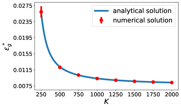
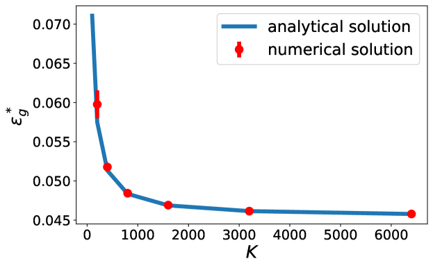
Figure 3: Asymptotic generalization error $\epsilon_{g}^{*}$ as a function of $K$ for $M=1$ for a error function as the activation with $N=200$ (top) and ReLU activation with $N=50$ (bottom). The numerical solution of Eq. (13) is obtained from ten initializations of random matrices $\bm{R}$ and $\bm{Q}$ under the linearized setup. The errorbars show the standard deviation of these averages. The analytical solution is based on Eq. (18) for the error function and on Eq. (18) for the ReLU activation.

Next, we evaluate the asymptotic generalization error for the ReLU activation function in the linearized regime. For this we linearize Eq. (3) and rewrite this again in a compact form

$$\epsilon_{g}^{*}=\frac{1}{4}-\frac{1}{2}\hat{\bm{R}}^{T}\hat{\bm{Q}}^{-1}\hat{\bm{R}}$$ (20)

with $\hat{Q}_{ii}=\frac{1}{2}$, $\hat{Q}_{ij}=Q_{ij}+\frac{1}{2\pi}$ and $\hat{R}_{i}=\frac{1}{4}R_{i}+\frac{1}{2\pi}$. As for the error function case, we take the expectation value of the r.h.s of Eq. (20) and use the definition of $\hat{\bm{R}}$

$$\left<\hat{\bm{R}}^{T}\hat{\bm{Q}}^{-1}\hat{\bm{R}}\right> =\frac{1}{16}\left<\bm{R}^{T}\hat{\bm{Q}}^{-1}\bm{R}\right>$$

$$+\frac{1}{8\pi}\left[\left<\bm{R}^{T}\bm{T}\right>+\left<\bm{T}^{T}\bm{R}\right>\right]$$

$$+\frac{1}{4\pi^{2}}\sum_{ij}\left(\hat{\bm{Q}}^{-1}\right)_{ij},$$ (21)

where $\bm{T}^{T}$ is a vector containing the sum of the columns of $\hat{\bm{Q}}^{-1}$, i.e. $T_{i}=\sum_{j}\left(\hat{\bm{Q}}^{-1}\right)_{ij}$. The second term of Eq. (21) vanishes as $\bm{R}$ occurs only linearly and $\left<\bm{R}\right>=0$. After exploiting the definition of $\bm{R}$ and that the entries of the teacher vector are i.i.d, we obtain for the first term of Eq. (21)

$$\left<\bm{R}^{T}\hat{\bm{Q}}^{-1}\bm{R}\right>=\frac{1}{N}\left<\text{tr}\left(\bm{Q}\hat{\bm{Q}}^{-1}\right)\right>.$$ (22)

With the help of the Sherman-Morrison formula, we can calculate $\hat{\bm{Q}}^{-1}$ and find

$$\hat{\bm{Q}}^{-1}=\bm{A}^{-1}-\frac{\bm{A}^{-1}vv^{T}\bm{A}^{-1}}{2\pi\left(1+\frac{1}{2\pi}v^{T}\bm{A}^{-1}v\right)}$$ (23)

with $\bm{A}=\frac{1}{4}\left(\bm{Q}+\mathbb{I}-\frac{2}{\pi}\mathbb{I}\right),v=\left(1,1,...,1\right)^{T}$ and $\mathbb{I}$ as the identity matrix. For the first part of the trace, we obtain with the same arguments as for the error function activation $\frac{1}{N}\left<\text{tr}\left(\bm{Q}\bm{A}^{-1}\right)\right>=\frac{1}{N}\sum_{i}^{K}\left<\frac{4\lambda_{i}}{\lambda_{i}+1-\frac{2}{\pi}}\right>$ and in the ultra-wide limit $\lim_{\frac{N}{K}\rightarrow 0}\lim_{K,N\rightarrow\infty}\frac{1}{N}\sum_{i}^{K}\left<\frac{4\lambda_{i}}{\lambda_{i}+1-\frac{2}{\pi}}\right>=4\hskip 2.0pt$. As shown in the Appendix, we find for the second part $\lim_{K,N\rightarrow\infty}\left<\frac{1}{N}\text{tr}\left(\frac{\bm{Q}\bm{A}^{-1}vv^{T}\bm{A}^{-1}}{2\pi\left(1+\frac{1}{2\pi}v^{T}\bm{A}^{-1}v\right)}\right)\right>\propto\frac{1}{N}\hskip 2.0pt$. Thus, we conclude

$$\lim_{\frac{N}{K}\rightarrow 0}\lim_{K,N\rightarrow\infty}\left<\bm{R}^{T}\hat{\bm{Q}}^{-1}\bm{R}\right>=4.$$ (24)

Now, we evaluate the third term given in Eq. (21). For this, we sum over the entries of $\hat{\bm{Q}}^{-1}$ with the help of Eq. (23). In the thermodynamic limit $N\rightarrow\infty$, we can assume $Q_{ij}+\frac{1}{2\pi}\approx\frac{1}{2\pi}$ since $Q_{ij}\propto\frac{1}{\sqrt{N}}$. Therefore, we obtain in this limit $\bm{A}\approx\left(\frac{1}{2}-\frac{1}{2\pi}\right)\mathbb{I}$ and for the sum

$$\sum_{ij}^{K}\left(\hat{\bm{Q}}^{-1}\right)_{ij} =Ka\left(1-\frac{Ka}{2\pi}\frac{1}{1+\frac{Ka}{2\pi}}\right)-\mathcal{O}\left(\frac{N}{K}\right)$$

$$\overset{\frac{N}{K}\rightarrow 0}{\underset{K,N\rightarrow\infty}{=}}2\pi.$$ (25)

with $a=\frac{1}{\frac{1}{2}-\frac{1}{2\pi}}$. After inserting Eqs. (24) and (25) into Eq. (20), we obtain for the asymptotic generalization error in the linearized regime

$$\lim_{\frac{N}{K}\rightarrow 0}\lim_{K,N\rightarrow\infty}\left<\epsilon_{g_{\mathrm{ReLU}}}^{*}\right>=\frac{1}{8}-\frac{1}{4\pi}\approx 0.045$$ (26)

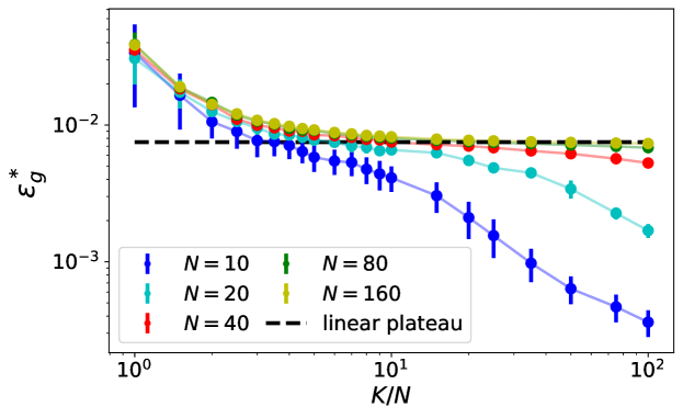
Figure 4: Asymptotic generalization error as a function of $\frac{K}{N}$ for an error activation $g\left(x\right)=\mathrm{erf}\left(\frac{x}{\sqrt{2}}\right)$ (top) and ReLU (bottom). Here, we evaluate Eq. (13) numericall and compute the expectation value of the generalization error for a given $\frac{K}{N}$. The errorbars show the standard deviation of the average over $100$ initializations for $N=10$ and $10$ initializations for $N>10$. The asymptotic generalization error increases with $N$, even though the hidden layer size increases proportional to that of the input layer. For large enough $N$ and finite $\frac{K}{N}$, the generalization error obtains the limit value for the linearized scenario given in Eq. (19) for the error function and Eq. (26) for the ReLU activation function.

Figure (3) shows the asymptotic generalization error given by Eq. (18) together the corresponding numerical solution of the expectation value averaged over different initializations of $\bm{R}$ and $\bm{Q}$ in the linearized setting. Figure (4) displays the numerical solution of Eq. (13) for the error function averaged over several matrix initializations not restricted to the linearized setting and shows how the linearized regime is reached in regard of the ratio $\frac{K}{N}$. For small ratios, we are in the linearized regime for which we have small correlations between the student and teacher vectors whereas for large enough ratios, one obtains a transition where linearization is no longer valid. However, the point of transition is different for different ratios depending on the input dimension $N$ and is shifted to the right as $N$ increases. Therefore, we conclude that the linearized regime is indeed valid for $N,K\rightarrow\infty$ under a fixed and finite ratio.

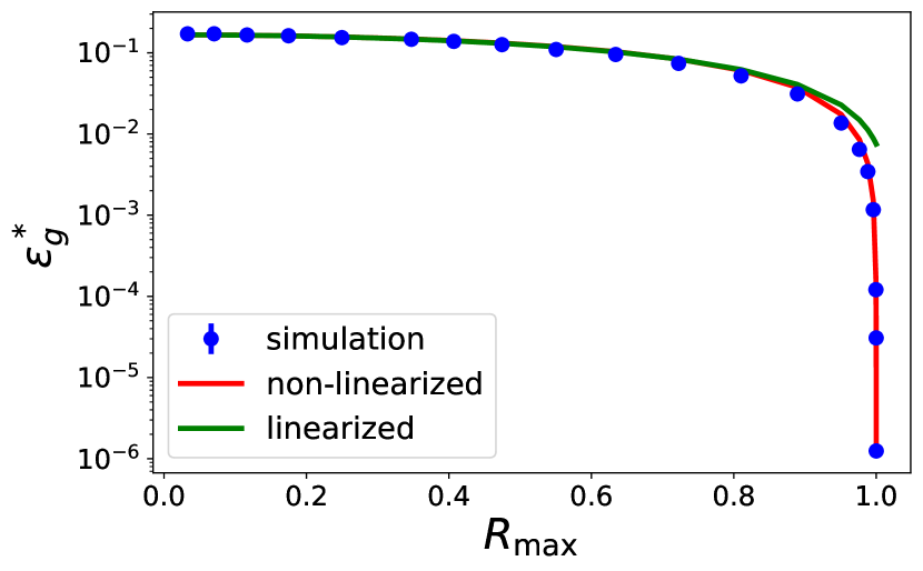
Figure 5: Asymptotic generalization error as a function of $R_{\mathrm{max}}=\max_{1\leq i\leq K}\hskip 2.0ptR\in\{R_{i}\}$ for $K=7$, $M=1$, $N=5$ and $\eta=\frac{0.1}{K}$ for a error function as the activation $g\left(x\right)=\mathrm{erf}\left(\frac{x}{\sqrt{2}}\right)$. We initialize the student and set the teacher in such a way that the first component of $\bm{R}$ is the largest one and the other are small and of similar size. The blue curve shows the corresponding simulation. The orange and green curves show the solution of Eq. (13) for a perceptron and a linearized perceptron, respectively. For the simulation, we averaged the generalization error over a predefined interval to get its asymptotic value. The errorbars (standard deviation of this average) are smaller than the symbol size.

6 Perfect Learning Scenario

Numerically, it turns out that for a constant $N$ and increasing $K$ the asymptotic generalization error decreases towards zero (cf. Figure (4)). However, for a constant ratio $\frac{K}{N}$ the generalization error increases as the input size $N$ becomes larger meaning that the student size $K$ is not big enough to maintain a small generalization error. The reason for that lies in the probability distribution of the overlaps $R_{i}$. The larger the student size $K$ becomes, the higher is the probability to pick a student vector that has a high overlap with the teacher vector under a constant input size $N$. The remaining problem is to figure out how fast the student size $K$ must grow with $N$ to obtain a small asymptotic generalization error. Accompanying this, the more student vectors are approximately in the direction of the teaching vector, the smaller the generalization error is in general, making a linearization of $\hat{\bm{R}}$ and $\hat{\bm{Q}}$ infeasible. Moreover, if only one student vector shows a high overlap, then the generalization error already decreases towards zero as $R_{i}\rightarrow 1$ (cf. Figure (5)).
Therefore, we ask for the probability to find at least one large overlap $\mathrm{max}\{R_{i}\}>R^{*}$ after the initialization of $K$ student vectors for a given $N$ and threshold $R^{*}$. We use the relation

$$P\left(\mathrm{max}\{R_{i}\}>R^{*};N,K\right)=1-F\left(R^{*};N\right)^{K},$$ (27)

where $F\left(R^{*};N\right)=\mathrm{Pr}\left(R\leq R^{*};N\right)=\int_{0}^{R^{*}}dR_{i}\hskip 2.0pt\rho\left(R_{i}\right)$ is the cumulative probability to find $R\leq R^{*}$ after randomly drawing a student vector, obtained by integrating over a density function $\rho\left(R\right)$. Since the student and teacher vectors are drawn from a uniform distribution over the $N$-sphere, the shifted overlaps $\frac{R_{i}+1}{2}$ are generated by the beta distribution. For the error function activation, we obtain for the density $\rho\left(y\right)=\lvert\cos\left(y\right)\rvert\beta\left(\frac{2\sin\left(y\right)+1}{2};a,b\right)$, where $\beta\left(t;a,b\right)=\frac{1}{B(a,b)}t^{a-1}(1-t)^{b-1}$ is the beta density function with normalization constant $B(a,b)=\int_{0}^{1}t^{a-1}(1-t)^{b-1}\hskip 3.0ptdt$ and $a=b=\frac{N-1}{2}$. We can now perform the integration for $R^{*}>R$, thus obtaining the probability for large overlaps between student and teacher vectors

$$F\left(R^{*};N\right) =1-\int_{\arcsin\left(\frac{R^{*}}{2}\right)}^{\frac{\pi}{6}}\rho\left(y\right)\hskip 3.0ptdy$$

$$=\frac{B\left(\frac{R^{*}+1}{2},a,a\right)}{B\left(a,a\right)}$$

$$=I_{z}\left(a,a\right)\ .$$ (28)

Here, $B(z,\alpha,\beta)=\int_{0}^{z}t^{\alpha-1}(1-t)^{\beta-1}\hskip 3.0ptdt$ is the incomplete beta function with $z=\frac{R^{*}+1}{2}$ for the case above and $I_{z}\left(a,b\right)$ is the regularized incomplete beta function. Therefore, our cumulative distribution function is related to the Binomial cumulative distribution function via the regularized incomplete beta function $1-F\left(R^{*};N\right)=F_{\mathrm{Binomial}}\left(\frac{N-1}{2};N-2,\frac{R^{*}+1}{2}\right)$. For the case ${R^{*}}\lesssim 1$, one can estimate the tail bounds of the Binomial distribution function by the Chernoff bound $F_{\mathrm{Binomial}}\left(\frac{N-1}{2};N-2,\frac{R^{*}+1}{2}\right)\geq\frac{1}{\sqrt{2N-4}}\exp\left[-\left(N-2\right)D\left(\frac{N-3}{2N-4}\bigg{\|}\frac{R*+1}{2}\right)\right]$ with the Kullback-Leibler divergence $D\left(P\|Q\right)=P\ln\left(\frac{P}{Q}\right)+(1-P)\log\left(\frac{1-P}{1-Q}\right)$ (Robert, 1990).
Furthermore, we demand $P\left(\mathrm{max}\{R_{i}\}>R^{*};N,K\right)>P^{*}$, where $P^{*}$ is a probability threshold or confidence and insert this condition in Eq. (27) which yields $K=\frac{\ln\left(1-P^{*}\right)}{\ln\left(F\left(R^{*};N\right)\right)}$. Finally, we obtain

$$K>\sqrt{2N-4}\hskip 5.0pte^{\frac{N}{2}\ln\left(\frac{1}{1-{R^{*}}^{2}}\right)}\hskip 3.0pt\lvert\ln\left(1-P^{*}\right)\rvert\hskip 2.0pt.$$ (29)

Therefore, the student size $K$ has to increase exponentially fast with the input-layer size $N$ for a fixed $R^{*}$ and $P^{*}$ leading to exponetial long training times if one wants to keep a small generalizaton error below the threshold of the linearized regime. This result is consistent with the conclusions in (Yehudai & Shamir, 2019).

7 Conclusion

In conclusion, we have studied the learning dynamics of the random feature model trained by the stochastic gradient descent embedded in the student-teacher framework. We obtained asymptotic solutions of the generalization error out of a set of coupled differential equations describing the weight dynamics. For a regime with a finite ratio of hidden layer width and input dimension, we computed the asymptotic generalization error and found that it stays finite for two choices of activation functions. In the second part of this work, we found by a simple ansatz that the generalization error can become arbitrarily small under an exponential increase of the student size in relation to the input dimension.

8 Appendix

The code for this work can be find here.

8.1 Exact expressions for the system

In order to derive the exact expression for the generalization error $\epsilon_{g}=\left<\epsilon\left(c_{i},\bm{\xi}\right)\right>_{\bm{\xi}}$ and the differential equations, we introduce local fields $x_{i}^{\mu}=\frac{\bm{J}_{i}^{\mu}\bm{\xi^{\mu}}}{\sqrt{N}},y_{n}^{\mu}=\frac{\bm{B}_{n}\bm{\xi}^{\mu}}{\sqrt{N}}$. These local fields describe the overlaps between the student and teacher vectors with the input vector. Due to the special form of the mean squared loss function, we obtain the following structure for the generalization error

$$\epsilon_{g}= \frac{1}{2}\sum_{i,j}^{K}c_{i}c_{j}I_{2}(i,j)+\frac{1}{2M}\sum_{n,m}^{M}I_{2}(n,m)$$

$$-\frac{1}{\sqrt{M}}\sum_{i}^{K}\sum_{n}^{M}c_{i}I_{2}(i,n)$$ (30)

with $I_{2}(i,j)=\tilde{\bm{Q}}=\left<g\left(x_{i}\right)g\left(x_{j}\right)\right>_{\xi},I_{2}(i,n)=\tilde{\bm{R}}=\left<g\left(x_{i}\right)g\left(y_{n}\right)\right>_{\xi}$. Therefore, the exact generalization error depends on the choice of the activation function.
The expressions $I_{2}$ are integrals over the local fields which are solved in closed form for error activation functions by (Saad & Solla, 1995b; Goldt et al., 2019) and for a ReLU function in (Oostwal et al., 2021) for the soft committee machine. For example, one finds for the error activation function a $2\times 2-$ sub-covariance matrix, which contains the relevant terms

$$I_{2}=\frac{2}{\pi}\;\arcsin\left(\frac{C_{12}}{\sqrt{1+C_{11}}\sqrt{1+C_{22}}}\right)$$ (31)

and for the ReLU function

$$I_{2}= \frac{C_{12}}{4}+$$

$$\frac{1}{2\pi}\biggl{[}\sqrt{C_{11}C_{12}-C_{12}^{2}}+C_{12}\arcsin\left(\frac{C_{12}}{\sqrt{C_{11}C_{22}}}\right)\biggr{]}.$$ (32)

For example, one obtains the following sub-matrix for the student-student overlaps

$$C(i,k)=\left(\begin{array}[]{ccc}Q_{ii}&Q_{ik}\\ Q_{ik}&Q_{kk}\\ \end{array}\right).$$ (33)

One can solve the expectation values analytically for both activation functions with the integral terms $I_{2}$. For the error function, one finds for the generalization error (Saad & Solla, 1995b; Goldt et al., 2019)

$$\epsilon_{g} =\frac{1}{\pi}\Biggl{[}\sum_{i,j}{c_{i}c_{j}\arcsin{\left(\frac{Q_{ij}}{\sqrt{1+Q_{ii}}\sqrt{1+Q_{jj}}\ }\right)}}$$

$$+\frac{1}{M}\sum_{n,m}{\arcsin{\left(\frac{T_{nm}}{\sqrt{1+T_{nn}}\sqrt{1+T_{mm}}\ }\right)}}$$

$$-\frac{2}{\sqrt{M}}\sum_{i,n}{c_{i}\arcsin{\left(\frac{R_{in}}{\sqrt{1+Q_{ii}}\sqrt{1+T_{nn}}\ }\right)}}\Biggr{]}.\vspace{7pt}$$ (34)

and for a ReLU activation (Oostwal et al., 2021)

$$\epsilon_{g}= \sum_{i,j}\frac{c_{i}c_{j}}{2}\biggl{[}\frac{Q_{ij}}{4}+$$

$$\frac{1}{2\pi}\biggl{[}\sqrt{Q_{ii}Q_{jj}-Q_{ij}^{2}}+Q_{ij}\arcsin\left(\frac{Q_{ij}}{\sqrt{Q_{ii}Q_{jj}}}\right)\biggr{]}$$

$$-\sum_{i,n}\frac{c_{i}}{\sqrt{M}}\biggl{[}\frac{R_{in}}{4}+$$

$$\frac{1}{2\pi}\biggl{[}\sqrt{Q_{ii}T_{nn}-R_{in}^{2}}+R_{in}\arcsin\left(\frac{R_{in}}{\sqrt{Q_{ii}T_{nn}}}\right)\biggr{]}$$

$$+\sum_{n,m}\frac{1}{2M}\biggl{[}\frac{T_{nm}}{4}+$$

$$\frac{1}{2\pi}\biggl{[}\sqrt{T_{nn}T_{mm}-T_{nm}^{2}}+T_{nm}\arcsin\left(\frac{T_{nm}}{\sqrt{T_{nn}T_{mm}}}\right)\biggr{]}$$ (35)

For our setup $Q_{ii}=1,T_{nm}=\delta_{nm}$, and $M=1$, the expressions for the error activation and ReLU activation reduce to Eq. (2 )and Eq. (3), respectively. Furthermore, we can also insert these definitions into Eq. (11) in order to get the exact formula for the differential equations in both cases.

8.2 Relative variance estimation

We find for the relative variance

$$\frac{\left<\frac{d\bm{c}}{d\alpha}^{2}\right>-\left<\frac{d\bm{c}}{d\alpha}\right>^{2}}{\left<\frac{d\bm{c}}{d\alpha}\right>^{2}}=\frac{\eta^{2}}{K}\frac{\left<\nabla\epsilon^{2}\right>-\nabla\epsilon_{g}^{2}}{\nabla\epsilon_{g}^{2}}$$ (36)

$$=\frac{\eta^{2}}{K}\frac{\sum_{ij}^{K}\left<\left[\zeta-\sigma\right]^{2}g\left(x_{i}\right)g\left(x_{j}\right)\right>-\frac{4}{\pi^{2}}\left(\left(\tilde{Q}c-\tilde{R}\right)^{2}\right)_{ij}}{\frac{4}{\pi^{2}}\left(\left(\tilde{Q}c-\tilde{R}\right)^{2}\right)_{ij}}$$ (37)

In general, we assume $c_{i}\sim\frac{1}{\sqrt{K}}$, that is at least given for the initialization. For the first part of the sum, we know that $\left[\zeta-\sigma\right]\approx O\left(1\right)$ and assume that the student vectors are weakly correlated with joint variance of $\frac{1}{N}$. This gives

$$\sum_{ij}^{K}g\left(x_{i}\right)g\left(x_{j}\right)\approx O\left(\frac{K}{N}\right),$$ (38)

as a sum over random variables with random signs. For the second part of the summation, we obtain

$$\hat{c}_{i}=\sum_{j}^{K}\tilde{Q}_{ij}c_{j} \approx\frac{1}{\sqrt{K}}\left(O\left(1\right)+\sum_{j\neq i}^{K}\tilde{Q}_{ij}\right)$$

$$\approx O\left(\frac{1}{\sqrt{K}}\right)+O\left(\frac{1}{\sqrt{N}}\right),$$ (39)

where the remaining sum for $j\neq i$ is a sum over random variables with zero mean and a variance of $\frac{1}{N}$ . This leads to

$$\sum_{ij}^{K}\hat{c}_{i}\hat{c}_{j}\approx O\left(\frac{K}{N}\right),$$ (40)

as a sum over weakly correlated random variables. The last part leads to

$$\sum_{ij}^{K}\left(\tilde{R}\tilde{R}^{T}\right)_{ij}\approx O\left(\frac{K}{N}\right).$$ (41)

Finally, one finds for the scaling of the relative variance

$$\frac{\left<\frac{d\bm{c}}{d\alpha}^{2}\right>-\left<\frac{d\bm{c}}{d\alpha}\right>^{2}}{\left<\frac{d\bm{c}}{d\alpha}\right>^{2}}\propto\frac{1}{K}.$$ (42)

8.3 Details on the RFM with ReLU activation in the linearized regime

Here, we want to derive the estimation of the following expectation value

$$\left<\bm{R}^{T}\hat{\bm{Q}}^{-1}\bm{R}\right>=\frac{1}{N}\left<\text{tr}\left(\bm{Q}\hat{\bm{Q}}^{-1}\right)\right>.$$ (43)

, with $\hat{\bm{Q}}^{-1}=\bm{A}^{-1}-\frac{\bm{A}^{-1}vv^{T}\bm{A}^{-1}}{2\pi\left(1+\frac{1}{2\pi}v^{T}\bm{A}^{-1}v\right)}$. As mentioned in the main paper, this expectation value consists of two parts. The first part can be solved with similar steps as for the error activation function. In order to estimate $\lim_{K,N\rightarrow\infty}\left<\frac{1}{N}\text{tr}\left(\frac{\bm{Q}\bm{A}^{-1}vv^{T}\bm{A}^{-1}}{2\pi\left(1+\frac{1}{2\pi}v^{T}\bm{A}^{-1}v\right)}\right)\right>$, we express $\bm{A}^{-1}$ with the help of the Woodbury matrix identity

$$\bm{A}^{-1} =\frac{4}{1-\frac{2}{\pi}}\left[\bm{1}_{K}-\frac{1}{1-\frac{2}{\pi}}\frac{\bm{J}^{T}}{\sqrt{N}}\left(\bm{1}_{N}+\frac{1}{1-\frac{2}{\pi}}\frac{\bm{J}\bm{J}^{T}}{N}\right)^{-1}\frac{\bm{J}}{\sqrt{N}}\right]$$

$$=\frac{4}{1-\frac{2}{\pi}}\left[\bm{1}_{K}-\bm{C}\right]$$ (44)

with the student matrix $\bm{J}\in\mathbb{R}^{N\mathrm{x}K}$ and identity matrices in $K$-space $\bm{1}_{K}$ and $N$-space $\bm{1}_{N}$. Since $vv^{T}$ is a rank-1 matrix, the matrix $\bm{A}^{-1}vv^{T}\bm{A}^{-1}$ has still rank 1 and we can rewrite it

$$\bm{A}^{-1}\bm{v}\bm{v}^{T}\bm{A}^{-1}=\bm{u}\bm{u}^{T}$$ (45)

with $u_{i}=\frac{4}{1-\frac{2}{\pi}}\left[1-\sum_{l}^{K}C_{il}\right]$. Therefore, we have $\bm{Q}\bm{A}^{-1}vv^{T}\bm{A}^{-1}=\bm{Q}\bm{u}\bm{u}^{T}$, which is a rank-1 matrix with one eigenvalue that is not zero and we estimate $\lambda=\bm{u}^{T}\bm{Q}\bm{u}=\sum_{ij}u_{i}Q_{ij}u_{j}\approx\sum_{i}u_{i}^{2}=\mathcal{O}\left(K\right)$ for the leading order of the sum. For the denominator, we obtain $\bm{v}^{T}\bm{A}^{-1}\bm{v}\approx\mathcal{O}\left(K\right)$ and the therefore the statement in the main text follows.

References

- Advani et al. (2020) Advani, M. S., Saxe, A. M., and Sompolinsky, H. High-dimensional dynamics of generalization error in neural networks. Neural Networks, 132:428–446, 2020. ISSN 0893-6080. doi: https://doi.org/10.1016/j.neunet.2020.08.022. URL https://www.sciencedirect.com/science/article/pii/S0893608020303117.
- Arora et al. (2019a) Arora, S., Du, S., Hu, W., Li, Z., and Wang, R. Fine-grained analysis of optimization and generalization for overparameterized two-layer neural networks. In Chaudhuri, K. and Salakhutdinov, R. (eds.), Proceedings of the 36th International Conference on Machine Learning, volume 97 of Proceedings of Machine Learning Research, pp. 322–332. PMLR, 09–15 Jun 2019a. URL https://proceedings.mlr.press/v97/arora19a.html.
- Arora et al. (2019b) Arora, S., Du, S. S., Hu, W., Li, Z., Salakhutdinov, R. R., and Wang, R. On exact computation with an infinitely wide neural net. In Wallach, H., Larochelle, H., Beygelzimer, A., d'Alché-Buc, F., Fox, E., and Garnett, R. (eds.), Advances in Neural Information Processing Systems, volume 32. Curran Associates, Inc., 2019b. URL https://proceedings.neurips.cc/paper/2019/file/dbc4d84bfcfe2284ba11beffb853a8c4-Paper.pdf.
- Bahri et al. (2020) Bahri, Y., Kadmon, J., Pennington, J., Schoenholz, S. S., Sohl-Dickstein, J., and Ganguli, S. Statistical mechanics of deep learning. Annual Review of Condensed Matter Physics, 11(1):501–528, 2020. doi: 10.1146/annurev-conmatphys-031119-050745.
- Bartlett (1998) Bartlett, P. The sample complexity of pattern classification with neural networks: the size of the weights is more important than the size of the network. IEEE Transactions on Information Theory, 44(2):525–536, 1998. doi: 10.1109/18.661502.
- Belkin et al. (2019) Belkin, M., Hsu, D., Ma, S., and Mandal, S. Reconciling modern machine-learning practice and the classical bias–variance trade-off. Proceedings of the National Academy of Sciences, 116(32):15849–15854, 2019. doi: 10.1073/pnas.1903070116. URL https://www.pnas.org/doi/abs/10.1073/pnas.1903070116.
- Biehl & Schwarze (1995) Biehl, M. and Schwarze, H. Learning by on-line gradient descent. Journal of Physics A: Mathematical and General, 28(3):643, feb 1995. doi: 10.1088/0305-4470/28/3/018. URL https://dx.doi.org/10.1088/0305-4470/28/3/018.
- Biehl et al. (1996) Biehl, M., Riegler, P., and Wöhler, C. Transient dynamics of on-line learning in two-layered neural networks. Journal of Physics A: Mathematical and General, 29(16):4769, aug 1996. doi: 10.1088/0305-4470/29/16/005. URL https://dx.doi.org/10.1088/0305-4470/29/16/005.
- Biehl et al. (1998) Biehl, M., Schlösser, E., and Ahr, M. Phase transitions in soft-committee machines. Europhysics Letters, 44(2):261, oct 1998. doi: 10.1209/epl/i1998-00466-6. URL https://dx.doi.org/10.1209/epl/i1998-00466-6.
- Canziani et al. (2017) Canziani, A., Paszke, A., and Culurciello, E. An analysis of deep neural network models for practical applications, 2017. URL https://openreview.net/forum?id=Bygq-H9eg.
- Carleo et al. (2019) Carleo, G., Cirac, I., Cranmer, K., Daudet, L., Schuld, M., Tishby, N., Vogt-Maranto, L., and Zdeborová, L. Machine learning and the physical sciences. Rev. Mod. Phys., 91:045002, Dec 2019. doi: 10.1103/RevModPhys.91.045002. URL https://link.aps.org/doi/10.1103/RevModPhys.91.045002.
- Chizat et al. (2019) Chizat, L., Oyallon, E., and Bach, F. On lazy training in differentiable programming. In Wallach, H., Larochelle, H., Beygelzimer, A., d'Alché-Buc, F., Fox, E., and Garnett, R. (eds.), Advances in Neural Information Processing Systems, volume 32. Curran Associates, Inc., 2019. URL https://proceedings.neurips.cc/paper/2019/file/ae614c557843b1df326cb29c57225459-Paper.pdf.
- Cohen et al. (2021) Cohen, O., Malka, O., and Ringel, Z. Learning curves for overparametrized deep neural networks: A field theory perspective. Phys. Rev. Res., 3:023034, Apr 2021. doi: 10.1103/PhysRevResearch.3.023034. URL https://link.aps.org/doi/10.1103/PhysRevResearch.3.023034.
- D’Ascoli et al. (2020) D’Ascoli, S., Refinetti, M., Biroli, G., and Krzakala, F. Double trouble in double descent: Bias and variance(s) in the lazy regime. In III, H. D. and Singh, A. (eds.), Proceedings of the 37th International Conference on Machine Learning, volume 119 of Proceedings of Machine Learning Research, pp. 2280–2290. PMLR, 13–18 Jul 2020. URL https://proceedings.mlr.press/v119/d-ascoli20a.html.
- de G. Matthews et al. (2018) de G. Matthews, A. G., Hron, J., Rowland, M., Turner, R. E., and Ghahramani, Z. Gaussian process behaviour in wide deep neural networks. In International Conference on Learning Representations, 2018. URL https://openreview.net/forum?id=H1-nGgWC-.
- Engel & Van den Broeck (2001) Engel, A. and Van den Broeck, C. Statistical Mechanics of Learning. Cambridge University Press, 2001. doi: 10.1017/CBO9781139164542.
- Gardner (1988) Gardner, E. The space of interactions in neural network models. Journal of Physics A: Mathematical and General, 21(1):257, jan 1988. doi: 10.1088/0305-4470/21/1/030. URL https://dx.doi.org/10.1088/0305-4470/21/1/030.
- Gardner & Derrida (1989) Gardner, E. and Derrida, B. Three unfinished works on the optimal storage capacity of networks. Journal of Physics A : Mathematical and General, 22(12):1983–1994, 1989. doi: 10.1088/0305-4470/22/12/004. URL https://hal.science/hal-03285594.
- Geiger et al. (2020) Geiger, M., Spigler, S., Jacot, A., and Wyart, M. Disentangling feature and lazy training in deep neural networks. Journal of Statistical Mechanics: Theory and Experiment, 2020(11):113301, nov 2020. doi: 10.1088/1742-5468/abc4de. URL https://dx.doi.org/10.1088/1742-5468/abc4de.
- Geman et al. (1992) Geman, S., Bienenstock, E., and Doursat, R. Neural networks and the bias/variance dilemma. Neural Computation, 4(1):1–58, 1992. ISSN 0899-7667. URL http://portal.acm.org/citation.cfm?id=148062.
- Ghorbani et al. (2019) Ghorbani, B., Mei, S., Misiakiewicz, T., and Montanari, A. Limitations of lazy training of two-layers neural network. In Wallach, H., Larochelle, H., Beygelzimer, A., d'Alché-Buc, F., Fox, E., and Garnett, R. (eds.), Advances in Neural Information Processing Systems, volume 32. Curran Associates, Inc., 2019. URL https://proceedings.neurips.cc/paper/2019/file/c133fb1bb634af68c5088f3438848bfd-Paper.pdf.
- Ghorbani et al. (2021) Ghorbani, B., Mei, S., Misiakiewicz, T., and Montanari, A. Linearized two-layers neural networks in high dimension. The Annals of Statistics, 49(2):1029 – 1054, 2021. doi: 10.1214/20-AOS1990. URL https://doi.org/10.1214/20-AOS1990.
- Goldt et al. (2019) Goldt, S., Advani, M., Saxe, A. M., Krzakala, F., and Zdeborová, L. Dynamics of stochastic gradient descent for two-layer neural networks in the teacher-student setup. In Wallach, H., Larochelle, H., Beygelzimer, A., d'Alché-Buc, F., Fox, E., and Garnett, R. (eds.), Advances in Neural Information Processing Systems, volume 32. Curran Associates, Inc., 2019. URL https://proceedings.neurips.cc/paper/2019/file/cab070d53bd0d200746fb852a922064a-Paper.pdf.
- Goldt et al. (2020) Goldt, S., Mézard, M., Krzakala, F., and Zdeborová, L. Modeling the influence of data structure on learning in neural networks: The hidden manifold model. Phys. Rev. X, 10:041044, Dec 2020. doi: 10.1103/PhysRevX.10.041044. URL https://link.aps.org/doi/10.1103/PhysRevX.10.041044.
- Goodfellow et al. (2016) Goodfellow, I., Bengio, Y., and Courville, A. Deep Learning. MIT Press, 2016. http://www.deeplearningbook.org.
- Györgyi & Tishby (1990) Györgyi, G. and Tishby, N. Neural networks and spin glasses. World Scientific, Singapore, pp. 3–36, 1990.
- Hastie et al. (2022) Hastie, T., Montanari, A., Rosset, S., and Tibshirani, R. J. Surprises in high-dimensional ridgeless least squares interpolation. The Annals of Statistics, 50(2):949 – 986, 2022. doi: 10.1214/21-AOS2133. URL https://doi.org/10.1214/21-AOS2133.
- Hertz et al. (1991) Hertz, J., Krough, A., and Palmer, R. Introduction To The Theory Of Neural Computation, volume 44. West view Press, 12 1991. doi: 10.1063/1.2810360.
- Hu et al. (2019) Hu, W., Li, C. J., Li, L., and Liu, J.-G. On the diffusion approximation of nonconvex stochastic gradient descent. Annals of Mathematical Sciences and Applications, 4(1):3–32, 2019.
- Jacot et al. (2018) Jacot, A., Gabriel, F., and Hongler, C. Neural tangent kernel: Convergence and generalization in neural networks. In Bengio, S., Wallach, H., Larochelle, H., Grauman, K., Cesa-Bianchi, N., and Garnett, R. (eds.), Advances in Neural Information Processing Systems, volume 31. Curran Associates, Inc., 2018. URL https://proceedings.neurips.cc/paper/2018/file/5a4be1fa34e62bb8a6ec6b91d2462f5a-Paper.pdf.
- Kampen (2007) Kampen, N. V. Stochastic processes in physics and chemistry. North Holland, 2007.
- Krizhevsky et al. (2012) Krizhevsky, A., Sutskever, I., and Hinton, G. E. Imagenet classification with deep convolutional neural networks. In Pereira, F., Burges, C., Bottou, L., and Weinberger, K. (eds.), Advances in Neural Information Processing Systems, volume 25. Curran Associates, Inc., 2012. URL https://proceedings.neurips.cc/paper/2012/file/c399862d3b9d6b76c8436e924a68c45b-Paper.pdf.
- Latz (2021) Latz, J. Analysis of stochastic gradient descent in continuous time. Statistics and Computing, 31(4), jul 2021. ISSN 0960-3174. doi: 10.1007/s11222-021-10016-8. URL https://doi.org/10.1007/s11222-021-10016-8.
- LeCun et al. (2015) LeCun, Y., Bengio, Y., and Hinton, G. Deep learning. Nature, 521(7553):436, 2015.
- Lee et al. (2018) Lee, J., Sohl-dickstein, J., Pennington, J., Novak, R., Schoenholz, S., and Bahri, Y. Deep neural networks as gaussian processes. In International Conference on Learning Representations, 2018. URL https://openreview.net/forum?id=B1EA-M-0Z.
- Lee et al. (2019) Lee, J., Xiao, L., Schoenholz, S., Bahri, Y., Novak, R., Sohl-Dickstein, J., and Pennington, J. Wide neural networks of any depth evolve as linear models under gradient descent. In Wallach, H., Larochelle, H., Beygelzimer, A., d'Alché-Buc, F., Fox, E., and Garnett, R. (eds.), Advances in Neural Information Processing Systems, volume 32. Curran Associates, Inc., 2019. URL https://proceedings.neurips.cc/paper/2019/file/0d1a9651497a38d8b1c3871c84528bd4-Paper.pdf.
- Li & Sompolinsky (2021) Li, Q. and Sompolinsky, H. Statistical mechanics of deep linear neural networks: The backpropagating kernel renormalization. Phys. Rev. X, 11:031059, Sep 2021. doi: 10.1103/PhysRevX.11.031059. URL https://link.aps.org/doi/10.1103/PhysRevX.11.031059.
- Mandt et al. (2017) Mandt, S., Hoffman, M. D., and Blei, D. M. Stochastic gradient descent as approximate bayesian inference. J. Mach. Learn. Res., 18(1):4873–4907, jan 2017. ISSN 1532-4435.
- Marčenko & Pastur (1967) Marčenko, V. A. and Pastur, L. A. Distribution of eigenvalues for some sets of random matrices. Mathematics of the USSR-Sbornik, 1(4):457, apr 1967. doi: 10.1070/SM1967v001n04ABEH001994. URL https://dx.doi.org/10.1070/SM1967v001n04ABEH001994.
- Mei & Montanari (2022) Mei, S. and Montanari, A. The generalization error of random features regression: Precise asymptotics and the double descent curve. Communications on Pure and Applied Mathematics, 75(4):667–766, 2022. doi: https://doi.org/10.1002/cpa.22008. URL https://onlinelibrary.wiley.com/doi/abs/10.1002/cpa.22008.
- Mei et al. (2022) Mei, S., Misiakiewicz, T., and Montanari, A. Generalization error of random feature and kernel methods: Hypercontractivity and kernel matrix concentration. Applied and Computational Harmonic Analysis, 59:3–84, 2022. ISSN 1063-5203. Special Issue on Harmonic Analysis and Machine Learning.
- Naveh et al. (2021) Naveh, G., Ben David, O., Sompolinsky, H., and Ringel, Z. Predicting the outputs of finite deep neural networks trained with noisy gradients. Phys. Rev. E, 104:064301, Dec 2021. doi: 10.1103/PhysRevE.104.064301. URL https://link.aps.org/doi/10.1103/PhysRevE.104.064301.
- Neal (1996) Neal, R. M. Priors for Infinite Networks, pp. 29–53. Springer New York, New York, NY, 1996. ISBN 978-1-4612-0745-0. doi: 10.1007/978-1-4612-0745-0˙2. URL https://doi.org/10.1007/978-1-4612-0745-0_2.
- Neyshabur et al. (2019) Neyshabur, B., Li, Z., Bhojanapalli, S., LeCun, Y., and Srebro, N. The role of over-parametrization in generalization of neural networks. In International Conference on Learning Representations, 2019. URL https://openreview.net/forum?id=BygfghAcYX.
- Novak et al. (2019) Novak, R., Xiao, L., Bahri, Y., Lee, J., Yang, G., Abolafia, D. A., Pennington, J., and Sohl-dickstein, J. Bayesian deep convolutional networks with many channels are gaussian processes. In International Conference on Learning Representations, 2019. URL https://openreview.net/forum?id=B1g30j0qF7.
- Oostwal et al. (2021) Oostwal, E., Straat, M., and Biehl, M. Hidden unit specialization in layered neural networks: Relu vs. sigmoidal activation. Physica A: Statistical Mechanics and its Applications, 564:125517, 2021. ISSN 0378-4371. doi: https://doi.org/10.1016/j.physa.2020.125517. URL https://www.sciencedirect.com/science/article/pii/S0378437120308153.
- Opper (1994) Opper, M. Learning and generalization in a two-layer neural network: The role of the vapnik-chervonvenkis dimension. Phys. Rev. Lett., 72:2113–2116, Mar 1994. doi: 10.1103/PhysRevLett.72.2113. URL https://link.aps.org/doi/10.1103/PhysRevLett.72.2113.
- Rahimi & Recht (2007) Rahimi, A. and Recht, B. Random features for large-scale kernel machines. In Platt, J., Koller, D., Singer, Y., and Roweis, S. (eds.), Advances in Neural Information Processing Systems, volume 20. Curran Associates, Inc., 2007. URL https://proceedings.neurips.cc/paper/2007/file/013a006f03dbc5392effeb8f18fda755-Paper.pdf.
- Rahimi & Recht (2008) Rahimi, A. and Recht, B. Uniform approximation of functions with random bases. 2008 46th Annual Allerton Conference on Communication, Control, and Computing, pp. 555–561, 2008.
- Reents & Urbanczik (1998) Reents, G. and Urbanczik, R. Self-averaging and on-line learning. Phys. Rev. Lett., 80:5445–5448, Jun 1998. doi: 10.1103/PhysRevLett.80.5445. URL https://link.aps.org/doi/10.1103/PhysRevLett.80.5445.
- Richert et al. (2022) Richert, F., Worschech, R., and Rosenow, B. Soft mode in the dynamics of over-realizable online learning for soft committee machines. Phys. Rev. E, 105:L052302, May 2022. doi: 10.1103/PhysRevE.105.L052302. URL https://link.aps.org/doi/10.1103/PhysRevE.105.L052302.
- Riegler & Biehl (1995) Riegler, P. and Biehl, M. On-line backpropagation in two-layered neural networks. Journal of Physics A: Mathematical and General, 28(20):L507, oct 1995. doi: 10.1088/0305-4470/28/20/002. URL https://dx.doi.org/10.1088/0305-4470/28/20/002.
- Robert (1990) Robert, B. Ash. information theory, 1990.
- Rotskoff & Vanden-Eijnden (2022) Rotskoff, G. and Vanden-Eijnden, E. Trainability and accuracy of artificial neural networks: An interacting particle system approach. Communications on Pure and Applied Mathematics, 75:1889–1935, 09 2022. doi: 10.1002/cpa.22074.
- Saad (2000) Saad, D. On-line learning in neural networks. Journal of the American Statistical Association, 95, 12 2000. doi: 10.2307/2669811.
- Saad & Solla (1995a) Saad, D. and Solla, S. A. Exact solution for on-line learning in multilayer neural networks. Phys. Rev. Lett., 74:4337–4340, May 1995a. doi: 10.1103/PhysRevLett.74.4337. URL https://link.aps.org/doi/10.1103/PhysRevLett.74.4337.
- Saad & Solla (1995b) Saad, D. and Solla, S. A. On-line learning in soft committee machines. Phys. Rev. E, 52:4225–4243, Oct 1995b. doi: 10.1103/PhysRevE.52.4225. URL https://link.aps.org/doi/10.1103/PhysRevE.52.4225.
- Samarin et al. (2022) Samarin, M., Roth, V., and Belius, D. Feature learning and random features in standard finite-width convolutional neural networks: An empirical study. In Cussens, J. and Zhang, K. (eds.), Proceedings of the Thirty-Eighth Conference on Uncertainty in Artificial Intelligence, volume 180 of Proceedings of Machine Learning Research, pp. 1718–1727. PMLR, 01–05 Aug 2022. URL https://proceedings.mlr.press/v180/samarin22a.html.
- Schwarze & Hertz (1993) Schwarze, H. and Hertz, J. Generalization in fully connected committee machines. Europhysics Letters, 21(7):785, mar 1993. doi: 10.1209/0295-5075/21/7/012. URL https://dx.doi.org/10.1209/0295-5075/21/7/012.
- Seung et al. (1992) Seung, H. S., Sompolinsky, H., and Tishby, N. Statistical mechanics of learning from examples. Phys. Rev. A, 45:6056–6091, Apr 1992. doi: 10.1103/PhysRevA.45.6056. URL https://link.aps.org/doi/10.1103/PhysRevA.45.6056.
- Silver et al. (2017) Silver, D., Schrittwieser, J., Simonyan, K., Antonoglou, I., Huang, A., Guez, A., Hubert, T., Baker, L., Lai, M., Bolton, A., Chen, Y., Lillicrap, T., Hui, F., Sifre, L., van den Driessche, G., Graepel, T., and Hassabis, D. Mastering the game of go without human knowledge. Nature, 550:354–, October 2017. URL http://dx.doi.org/10.1038/nature24270.
- Theunissen et al. (2020) Theunissen, M., Davel, M., and Barnard, E. Benign interpolation of noise in deep learning. South African Computer Journal, 32, 12 2020. doi: 10.18489/sacj.v32i2.833.
- Watkin et al. (1993) Watkin, T. L. H., Rau, A., and Biehl, M. The statistical mechanics of learning a rule. Rev. Mod. Phys., 65:499–556, Apr 1993. doi: 10.1103/RevModPhys.65.499. URL https://link.aps.org/doi/10.1103/RevModPhys.65.499.
- Williams (1996) Williams, C. Computing with infinite networks. In Mozer, M., Jordan, M., and Petsche, T. (eds.), Advances in Neural Information Processing Systems, volume 9. MIT Press, 1996. URL https://proceedings.neurips.cc/paper/1996/file/ae5e3ce40e0404a45ecacaaf05e5f735-Paper.pdf.
- Yehudai & Shamir (2019) Yehudai, G. and Shamir, O. On the Power and Limitations of Random Features for Understanding Neural Networks. Curran Associates Inc., Red Hook, NY, USA, 2019.
- Yoshida & Okada (2020) Yoshida, Y. and Okada, M. Data-dependence of plateau phenomenon in learning with neural network—statistical mechanical analysis*. Journal of Statistical Mechanics: Theory and Experiment, 2020(12):124013, dec 2020. doi: 10.1088/1742-5468/abc62f. URL https://dx.doi.org/10.1088/1742-5468/abc62f.
- Zhang et al. (2021) Zhang, C., Bengio, S., Hardt, M., Recht, B., and Vinyals, O. Understanding deep learning (still) requires rethinking generalization. Commun. ACM, 64(3):107–115, feb 2021. ISSN 0001-0782. doi: 10.1145/3446776. URL https://doi.org/10.1145/3446776.