Mutual information of subsystems and the Page curve for Schwarzschild de-Sitter black hole

Abstract

In this work, we show that the two proposals associated to the mutual information of matter fields can be given for an eternal Schwarzschild black hole in de-Sitter spacetime. These proposals also depicts the status of associated entanglement wedges and their roleplay in obtaining the correct Page curve of radiation. The first proposal has been give for the before Page time scenario, which shows that the mutual information $I(R_{H}^{+}:R_{H}^{-})$ vanishes at a certain value of the observer’s time $t_{b_{H}}=t_{H}$ (where $t_{H}\ll\beta_{H}$). We claim that this is the Hartman-Maldacena time at which the entanglement wedge associated to $R_{H}^{+}\cup R_{H}^{-}$ gets disconnected and the fine-grained radiation entropy has the form $S(R_{H})\sim\log(\beta_{H})$. The second proposal depicts the fact that just after the Page time, when the replica wormholes are the dominating saddle-points, the mutual information $I(B_{H}^{+}:B_{H}^{-})$ vanishes as soon as the time difference $t_{a_{H}}-t_{b_{H}}$ equals the scrambling time. Holographically, this reflects that the entanglement wedge associated to $B_{H}^{+}\cup B_{H}^{-}$ jumps to the disconnected phase at this particular time-scale. Furthermore, these two proposals lead us to the correct time-evolution of the fine-grained entropy of radiation as portrayed by the Page curve. We have also shown that similar observations can be obtained for the radiation associated to the cosmological horizon.

Hawking radiation is one of the most fascinating and mysterious phenomena in theoretical physics, and it is caused by pair formation that takes place in the black hole’s near-horizon area Hawking (1975). This phenomenon has drawn a lot of attention in the context of modern theoretical physics. This is because, as a quantum mechanical radiation, its presence provides a clear indication of the microscopic physics underlying the general relativity theory. This has motivated to probe its quantum mechanical components, such von Neumann entropy Nielsen and Chuang (2000). However, the investigation of the von Neumann entropy of the Hawking radiation has in turn provided us with a paradox. The paradox can be described in the following way. It has been noted that the creation of a black hole, which results from the gravitational collapse of a massive shell, is associated to a pure state. This implies that the corresponding von Neumann entropy is zero. Additionally, according to the theory of unitary evolution, the final state at the end of the evaporation process must likewise be a pure state, meaning that the von Neumann entropy once again must vanish at the end of the evaporation process. Hawking’s semi-classical analysis, however, demonstrated that for an evaporating black hole, the von Neumann entropy of Hawking radiation is an ever-increasing quantity with regard to the observer’s time Hawking (1976a), and it does not disappear even if the black hole has completely evaporated.
There is another way to understand this current scenario which is more suitable for the case of an eternal black hole. The von Neumann entropy of radiation is an well-known example of fine-grained type of entropy and on the other other hand, the thermodynamic entropy of the black hole is a perfect example of coarse-grained type of entropy Bekenstein (1972, 1973); Hawking (1976b)). Further, as the state corresponding to the whole system (radiation subsystem $R$ + black hole subsystem $R^{c}$) is a pure state, the fine-grained entropy of radiation is equal to the fine-grained entropy of the black hole subsystem, that is $S_{vN}(R)=S_{vN}(R^{c})$. This observation together with the Hawking’s semi-classical analysis implies that after a certain amount of time, the fine-grained entropy of black hole subsystem will greater than the coarse-grained entropy of the black hole ($S_{vN}(R)>S_{BH}$). This fact is self-contradictory as the basic definition of coarse-grained entropy is associated to the fact that it is obtained by maximizing the fine-grained entropy over all possible states. The above mentioned observation provides us an entropic way to understand the paradoxical situation.
So a natural question arises regarding the correct time evolution of the von Neumann entropy of Hawking radiation. This was efficiently addressed by the so-called Page curve. The Page curve curve suggested that in order to satisfy the unitarity condition, the von Neumann entropy of the radiation shall start from zero and monotonically increase upto the Page time and then again drop down to zero, signifying the end of the evaporation process Page (1993, 2013). The contradiction only emerges after the Page time as after this particular time one usually gets $S_{vN}(R)>S_{BH}$. Numerous intriguing methods have been developed to handle this problem while taking into account the unitarity evolution of radiation Almheiri et al. (2013a, b); Lloyd and Preskill (2014); Papadodimas and Raju (2014). Recently, the idea of entanglement wedge reconstruction from Hawking radiation has proposed that certain regions in the interior of a black hole may be responsible for the fine-grained entropy of that radiation Penington (2020); Almheiri et al. (2019a, 2020a, b). These auxiliary areas are known as islands, and the surfaces at their ends are known as quantum extremal surfaces (QES) Engelhardt and Wall (2015); Engelhardt and Fischetti (2019); Akers et al. (2020); Wall (2014). It is to be mentioned that the quantum extremal surfaces are the quantum corrected classical extremal surfaces Ryu and Takayanagi (2006); Hubeny et al. (2007). The fine-grained entropy of the Hawking radiation in the presence of the island in the black hole interior is provided by

$$S(R)=\textrm{min}\leavevmode\nobreak\ \mathop{\textrm{ext}}_{\mathcal{\mathrm{I}}}\bigg{\{}\frac{\textrm{Area}(\partial I)}{4G_{N}}+S_{vN}(I\cup R)\bigg{\}}\leavevmode\nobreak\ .$$ (1)

From a semi-classical perspective, the islands come from the replica wormhole saddle points (with the appropriate boundary conditions) of the gravitational path integral, which occur as a result of the use of the replica method in dynamical gravitational background Almheiri et al. (2020b); Penington et al. (2022); Goto et al. (2021); Colin-Ellerin et al. (2021). Due to this remarkable observation, the island formulation has emerged as an important prescription to be studied Almheiri et al. (2021); Chen et al. (2020); Hashimoto et al. (2020); Hartman et al. (2020); Anegawa and Iizuka (2020); Dong et al. (2020); Balasubramanian et al. (2021); Raju (2022a); Alishahiha et al. (2021); Krishnan (2021); Krishnan et al. (2020); Azarnia et al. (2021); Yu and Ge (2022a); Aref’eva and Volovich (2021); He et al. (2022); Omidi (2022); Yu et al. (2022); Ahn et al. (2022); Yadav (2022); Du et al. (2022); Hosseini Mansoori et al. (2022); Ageev et al. (2022); Yu and Ge (2022b); Hu et al. (2022a).
It is important to note that while the majority of the above mentioned studies are restricted to the black holes in asymptotically flat or AdS spacetimes, the most recent finding indicates that our universe is of de-Sitter nature. Therefore, it makes sense to investigate the effect of the positive cosmological constant in context of the information paradox problem. Keeping this in mind, we will consider the eternal Schwarzschild de-Sitter (SdS) spacetime as the black hole spacetime in this paper. Given that these black holes are formed during the early inflationary stage of our universe, the information paradox problem for the Schwarzschild de-Sitter black holes is crucial. It also offers an ideal toy model for global structures of isolated black holes in our universe, keeping in mind the current phase of our universe’s accelerated expansion. There are also causally disconnected areas in de-Sitter space, which is similar to the situation with black holes. Therefore, an observer may only access the regions of the universe that are enclosed by their own horizon. Furthermore, the cosmological event horizons emit and take in radiation similar to the black hole (Gibbons-Hawking radiation). In general, the entropy creation of the cosmological horizon is an observer-dependent feature in contrast to the black hole. It is caused by a lack of knowledge about what exists outside of the cosmic horizon. In this work, we will try to obtain the correct Page curve for the black hole horizon of the SdS black hole and the Page-like curve for the cosmological horizon of the same black hole. We shall do this by keeping in mind the island formulation. It is also to be mentioned that apart from the approach (gravitational set up) which we have followed in this work, there is another way (gravitational set up) to address this entropic paradox. This is known as the doubly holographic set up Takayanagi (2011); Fujita et al. (2011); Nozaki et al. (2012); Miao et al. (2017); Geng and Karch (2020); Geng et al. (2021a, b); Hu et al. (2022b); Geng et al. (2022a). Some very interesting works in this set up can be found in Almheiri et al. (2019a); Chen et al. (2020); Rozali et al. (2020); Almheiri et al. (2020c); Bousso and Wildenhain (2020); Afrasiar et al. (2023, 2022); Guo et al. (2023); Miao (2023); Hu et al. (2022a).
In Saha et al. (2022); Roy Chowdhury et al. (2022) it was shown that the mutual information of various subsystems plays a crucial role in obtaining the correct Page curve of Hawking radiation. To be precise, in Saha et al. (2022) it was shown that just after the Page time the mutual information of matter fields localized on $R_{+}$ and $R_{-}$ intervals vanishes, which eventually leads to a time-independent profile of fine-grained entropy $S(R)$. Furthermore, in Roy Chowdhury et al. (2022) the previous observation was exploited in detail and two proposals were given regarding the saturation of mutual information (of various subsystems) for two different time domains (before and after the Page time). However, these works were only restricted to the eternal black holes in AdS and asymptotically flat spacetime. In this work, we shall see whether these proposals hold for eternal black holes in de-Sitter spacetime or not. We would like to mention that our work does not take into account certain subtleties in graviational theories, for example diffeomorphism invariance, which enables an arbitrary definition of a subregion. A discussion on this aspect can be found in Geng et al. (2021c, 2022b); Raju (2022b) which shows that it can have important implications to quantum gravity.

I Brief discussion on the Kottler spacetime

The Schwarzschild de-Sitter (SdS) spacetime metric is the unique solution of Einstein’s vacuum field equation with positive cosmological constant in $(3+1)$- spacetime dimensions. This solution is sometimes also denoted as the Kottler solution. The metric of the SdS solution has the following form Kottler (1918)

$$ds^{2} = -f(r)dt^{2}+\frac{dr^{2}}{f(r)}+r^{2}(d\theta^{2}+\sin^{2}\theta d\phi^{2});$$

$$f(r) = 1-\frac{2M}{r}-\frac{\Lambda r^{2}}{3}\leavevmode\nobreak\$$ (2)

where $M$ is the mass parameter and $\Lambda$ is the cosmological constant. The above given lapse function in terms of the AdS radius can be recast as

$$f(r)=1-\frac{2M}{r}-\frac{r^{2}}{L^{2}_{\mathrm{AdS}}}\leavevmode\nobreak\ \leavevmode\nobreak\ .$$ (3)

We can recover the asymptotically flat Schwarzschild spacetime in the limit $\Lambda\rightarrow 0$ (or $L_{\mathrm{AdS}}\rightarrow\infty$).
We shall now discuss about the horizon structure of the Kottler metric. One can show that the horizon structure depends on the value of the cosmological constant $(\Lambda)$ as there exists a critical value of $\Lambda=\Lambda_{crit}=\frac{1}{9M^{2}}$ above which there event horizon does not exists and the corresponding solution is then denoted as the naked singularity. However, in the range $0<\Lambda<\Lambda_{crit}$ (or $\frac{m}{L_{\mathrm{AdS}}}<\frac{1}{3\sqrt{3}}$), there are three solutions for $f(r)=0$. Out of these three solutions only two are physical solutions Kottler (1918); Gibbons and Hawking (1977), one is known as the black hole horizon $(r_{H})$ and the other one is known as the cosmological horizon $(r_{c})$, $r_{c}>r_{H}$. Furthermore, in the limit $\Lambda\rightarrow\Lambda_{crit}$ there is a degenerate horizon Kottler (1918). In this work, we will only consider the range $0<\Lambda<\Lambda_{crit}$ along with the following form of the lapse function Goswami and Narayan (2022)

$$f(r)=\frac{1}{L_{\mathrm{AdS}}^{2}r}(r_{H}-r)(r-r_{c})(r+r_{H}+r_{c})\leavevmode\nobreak\ .$$ (4)

The expressions for the $r_{H}$ and $r_{c}$ (in terms of the mass parameter and the cosmological constant) are obtained to be Gibbons and Hawking (1977); Bhattacharya and Lahiri (2013); Yadav and Joshi (2023)

$$r_{H} = \frac{2}{\sqrt{\Lambda}}\cos\left(\frac{\pi}{3}+\frac{\arccos(3M\sqrt{\Lambda})}{3}\right)$$

$$r_{c} = \frac{2}{\sqrt{\Lambda}}\cos\left(\frac{\pi}{3}-\frac{\arccos(3M\sqrt{\Lambda})}{3}\right)\leavevmode\nobreak\ .$$ (5)

In order to proceed further, we shall now rewrite the metric in the Kruskal coordinates. As there are two different choices available for the horizons, there exists two different sets of Kruskal coordinates. This is due to the reason that the Kruskal coordinate transformations contain surface gravity in the expression which has different values corresponding to the different event horizons. This we denote as $\kappa_{H}$ (associated to the black hole horizon $r_{H}$) and $\kappa_{c}$ (associated to the cosmological horizon $r_{c}$). Keeping this mind, one can show two alternative forms of the metric in terms of the two different Kruskal coordinates. This can be represented as black horizon representation of the metric and the cosmological horizon description of the metric.
In order to obtain the form of the metric in the Kruskal coordinates, we first introduce the tortoise coordinate which satisfies the following transformation

$$u = t-r^{*}(r)\leavevmode\nobreak\ ,\leavevmode\nobreak\ v=t+r^{*}(r)$$ (6)

where $r^{*}(r)$ is the tortoise coordinate, given as

$$r^{*}(r)=\alpha_{H}\ln(|r_{H}-r|)-\alpha_{c}\ln(|r-r_{c}|)+\alpha^{\prime}\ln(r+r_{H}+r_{c}).$$ (7)

The expressions of $\alpha_{H}$, $\alpha_{c}$ and $\alpha^{\prime}$ read

$$\alpha_{H} = \frac{L^{2}_{\mathrm{AdS}}r_{H}}{(r_{c}-r_{H})(2r_{H}+r_{c})}$$

$$\alpha_{c} = \frac{L^{2}_{\mathrm{AdS}}r_{c}}{(r_{c}-r_{H})(2r_{c}+r_{H})}$$

$$\alpha^{\prime} = \frac{L^{2}_{\mathrm{AdS}}(r_{H}+r_{c})}{(2r_{c}+r_{H})(2r_{H}+r_{c})}\leavevmode\nobreak\ .$$ (8)

We first introduce the black hole horizon description of the metric. For the right wedge of the black hole horizon, the Kruskal coordinates read

$$U_{H} = -e^{-\kappa_{H}(t-r^{*}(r))}$$

$$V_{H} = e^{\kappa_{H}(t+r^{*}(r))}$$ (9)

and for the left wedge it read

$$U_{H} = e^{\kappa_{H}(t+r^{*}(r))}$$

$$V_{H} = -e^{-\kappa_{H}(t-r^{*}(r))}$$ (10)

where $\kappa_{H}$ is the surface gravity associated to black hole horizon

$$\kappa_{H}=\frac{(r_{c}-r_{H})(2r_{H}+r_{c})}{2L^{2}_{\mathrm{AdS}}r_{H}}\leavevmode\nobreak\ .$$ (11)

Further, one can obtain the following form of the Hawking temperature associated to the black hole horizon

$$T_{H}=\frac{\kappa_{H}}{2\pi}=\frac{(r_{c}-r_{H})(2r_{H}+r_{c})}{4\pi L^{2}_{\mathrm{AdS}}r_{H}}=\frac{1}{\beta_{H}}\leavevmode\nobreak\ .$$ (12)

In terms of the cosmological constant and the mass parameter, the surface gravity $(\kappa_{H})$ and Hawking temperature associated to the black hole horizon read Yadav and Joshi (2023)

$$\kappa_{H} = \sqrt{\Lambda}\left[\frac{1}{4\cos\left(\frac{1}{3}\arccos(3M\sqrt{\Lambda})+\frac{\pi}{3}\right)}-\cos\left(\frac{1}{3}\arccos(3M\sqrt{\Lambda})+\frac{\pi}{3}\right)\right]$$ (13)

$$T_{H} = \frac{\sqrt{\Lambda}}{2\pi}\left[\frac{1}{4\cos\left(\frac{1}{3}\arccos(3M\sqrt{\Lambda})+\frac{\pi}{3}\right)}-\cos\left(\frac{1}{3}\arccos(3M\sqrt{\Lambda})+\frac{\pi}{3}\right)\right]\leavevmode\nobreak\ .$$ (14)

On the other hand, the Bekenstein-Hawking entropy for the black hole horizon is given by $S_{BH}=\frac{\pi r_{H}^{2}}{G_{N}}$. Finally, the black horizon description of the metric in terms of the Kruskal coordinate reads

$$ds^{2}=-F^{2}(r)dU_{H}dV_{H}+r^{2}\Omega^{2}_{2}\leavevmode\nobreak\ ;\leavevmode\nobreak\ F^{2}(r)=\frac{f(r)}{\kappa_{H}^{2}}e^{-2\kappa_{H}r^{*}(r)}$$

where the detailed expression of $F(r)$ has the following form

$$F(r)=\frac{2L_{\mathrm{AdS}}r_{H}}{\sqrt{r}}\frac{|r-r_{c}|^{\frac{1}{2}(1+\frac{r_{c}}{r_{H}}\left(\frac{2r_{H}+r_{c}}{2r_{c}+r_{H}}\right))}(r+r_{c}+r_{H})^{\frac{1}{2}(1-\frac{r_{c}^{2}-r_{H}^{2}}{r_{H}(2r_{c}+r_{H})})}}{(2r_{H}+r_{c})(r_{c}-r_{H})}\leavevmode\nobreak\ .$$ (16)

We noe move on to describe the metric in terms of the cosmological horizon. The Kruskal coordinates for the right wedge of the cosmological horizon read

$$U_{c} = -e^{-\kappa_{c}(t-r^{*}(r))}$$

$$V_{c} = e^{\kappa_{c}(t+r^{*}(r))}$$ (17)

and for the left wedge, it read

$$U_{c} = e^{\kappa_{c}(t+r^{*}(r))}$$

$$V_{c} = -e^{-\kappa_{c}(t-r^{*}(r))}\leavevmode\nobreak\ .$$ (18)

The surface gravity $(\kappa_{c})$ and the Hawking temperature associated to the cosmological horizon have the following respective forms

$$\kappa_{c} = \frac{(r_{c}-r_{H})(2r_{c}+r_{H})}{2L^{2}_{\mathrm{AdS}}r_{c}}$$ (19)

$$T_{c} = \frac{\kappa_{c}}{2\pi}=\frac{(r_{c}-r_{H})(2r_{c}+r_{H})}{4\pi L^{2}_{\mathrm{AdS}}r_{c}}=\frac{1}{\beta_{c}}\leavevmode\nobreak\ .$$ (20)

The form of $\kappa_{c}$ and $T_{c}$ in terms of the cosmological constant and mass parameter are given as Yadav and Joshi (2023)

$$\kappa_{c} = \sqrt{\Lambda}\left[\frac{1}{4\cos\left(\frac{1}{3}\arccos(3M\sqrt{\Lambda})-\frac{\pi}{3}\right)}-\cos\left(\frac{1}{3}\arccos(3M\sqrt{\Lambda})-\frac{\pi}{3}\right)\right]$$ (21)

$$T_{c} = \frac{\sqrt{\Lambda}}{2\pi}\left[\frac{1}{4\cos\left(\frac{1}{3}\arccos(3M\sqrt{\Lambda})-\frac{\pi}{3}\right)}-\cos\left(\frac{1}{3}\arccos(3M\sqrt{\Lambda})-\frac{\pi}{3}\right)\right]\leavevmode\nobreak\ .$$ (22)

Therefore the cosmological horizon description of the metric in terms of the Kruskal coordinates can be written down as

$$ds^{2}=-G^{2}(r)dU_{c}dV_{c}+r^{2}d\Omega_{2}^{2}\leavevmode\nobreak\ ;\leavevmode\nobreak\ G^{2}(r)=\frac{f(r)}{\kappa_{c}^{2}}e^{-2\kappa_{c}r^{*}(r)}$$

where the conformal factor $G(r)$ has the following form

$$G(r)=\frac{2L_{\mathrm{AdS}}r_{c}}{\sqrt{r}}\frac{|r_{H}-r|^{\frac{1}{2}\left(1-\frac{r_{H}}{r_{c}}\frac{r_{H}+2r_{c}}{r_{c}+2r_{H}}\right)}(r+r_{c}+r_{H})^{\frac{1}{2}(1+\frac{r_{c}^{2}-r_{H}^{2}}{r_{c}(2r_{H}+r_{c})})}}{(r_{c}-r_{H})(2r_{c}+r_{H})}\leavevmode\nobreak\ .$$ (24)

Figure 1: Penrose-Carter diagram of Schwarzschild de-Sitter spacetime. In the above, $r=r_{H}$ represents the black hole event horizon and $r=r_{c}$ is the cosmological event horizon.

The above mentioned two alternative descriptions of the SdS metric can be understood in terms of the Penrose-Carter diagrams. This we provide in Fig.(1) where two physical horizons have been pointed out either of which can be used to describe the spacetime equivalently. In this work, our aim is to study the Page curve of radiation associated to both Hawking radiation and Gibbons-Hawking radiation. This can be done by isolating different patches of the spacetime by introducing the thermal opaque membrane Saida (2009); Ma et al. (2017); Sekiwa (2006a); Gomberoff and Teitelboim (2003); Bhattacharya and Joshi (2022); Sekiwa (2006b). These patches have been denoted as the black hole patch and the cosmological patch in the literature. We have shown this in Fig.(2).

Black hole patch

Cosmological patch

Figure 2: SAdS spacetime with thermal opaque membrane.

The principal reason behind introducing this thermal opaque membrane lies in the fact that we do not have any Kruskal coordinates which can remove the coordinate singularities simultaneously from both the black hole horizon and the cosmological horizon. On the other hand for the Schwarzschild de-Sitter spacetime the two horizons, namely the back hole horizon and the cosmlogical horizon can be thought as two different thermodynamic systems with different temperatures. Therefore they are not in the thermal equilibrium. For non-equilibrium system it is very much difficult to study its thermodynamic properties. Therefore to make the analysis simpler one has to ensure that the system (either the black hole horizon or the cosmological horizon) is in thermal equilibrium. The thermal opaque membrane does this job Saida (2009); Ma et al. (2017); Sekiwa (2006a); Gomberoff and Teitelboim (2003); Bhattacharya and Joshi (2022); Sekiwa (2006b). In a multi horizon spacetime one can use thermal opaque membrane to analyse one horizon by taking the other one as boundary. One can understand this thermal opaque membrane by following the approach given in Yadav and Joshi (2023); Bhattacharya and Joshi (2022).
Let us consider the radial part of the Klein-Gordon equation in SdS spacetime, which is found to be Yadav and Joshi (2023); Bhattacharya and Joshi (2022)

$$\left(-\frac{\partial^{2}}{\partial t^{2}}+\frac{\partial^{2}}{\partial r^{*2}}\right)\psi(r)+V_{eff}(r)\psi(r)=0\leavevmode\nobreak\ \leavevmode\nobreak\ .$$ (25)

The explicit form of the effective potential $(V_{eff})$ can be obtained by using the lapse function given in eq.(I). This reads Yadav and Joshi (2023); Bhattacharya and Joshi (2022)

$$V_{eff}=\left(1-\frac{2M}{r}-\frac{\Lambda r^{2}}{3}\right)\left(\frac{l(l+1)}{r^{2}}+\frac{2M}{r^{3}}-\frac{\Lambda}{3}\right)\leavevmode\nobreak\ .$$

One can show that the above expression vanishes for both the black hole horizon and the cosmological horizon. In Yadav and Joshi (2023); Bhattacharya and Joshi (2022) it was shown that this effective potential can be treated as the partition between the black hole and cosmological horizons. To understand this in the Penrose diagram one can introduce the Kruskal time-like and space-like coordinates for the black hole patch as

$$U_{H}=T_{H}-R_{H}\leavevmode\nobreak\ ,\leavevmode\nobreak\ V_{H}=T_{H}+R_{H}$$ (26)

and similarly for the cosmological patch

$$U_{c}=T_{c}-R_{c}\leavevmode\nobreak\ ,\leavevmode\nobreak\ V_{c}=T_{c}+R_{c}\leavevmode\nobreak\ .$$ (27)

By using this above Kruskal time-like and space-like coordinates, one can obtain the following Yadav and Joshi (2023)

$$-U_{H}V_{H} = R_{H}^{2}-T_{H}^{2}=e^{2\kappa_{H}r^{*}(r)}$$ (28)

$$-U_{c}V_{c} = R_{c}^{2}-T_{c}^{2}=e^{2\kappa_{c}r^{*}(r)}\leavevmode\nobreak\ .$$ (29)

The above results suggest that for $r=constant$, a hyperbola (membrane) in the $R_{H(c)}-T_{H(c)}$ plane can be realized in both the black hole and the cosmological patch.
On the other hand, it has been suggested that the analogue of “defect” in wedge holography is nothing but the “thermal opaque membrane” in Schwarzschild de-Sitter eternal black hole. Gravity may be considered to be sufficiently weak at these membranes because the membrane in question is far from the black hole/de-Sitter patch. We now proceed to investigate the role of mutual information of various subsystems in the Page curve associated to a multi-event horizon black hole spacetime.

II Analysis for the black hole patch

We now proceed to study the Page curve of Hawking radiation for the SdS eternal black hole in $3+1$ dimensions. As we have mentioned already, in order to probe the Hawking radiation we need to restrict ourselves to the black hole patch by introducing the thermal opaque membrane to freeze the cosmological horizon. We shall work with the form of the metric given in eq.(I) which corresponds to the black hole horizon description of the SdS solution.
On the other hand, we assume that the whole spacetime is filled with conformal matter of central charge $c$. To be more precise, we will consider the matter to be a free CFT. We will incorporate the $s$-wave approximation in conformal matter sector Polchinski (2017); Hubeny et al. (2010); Hashimoto et al. (2020). The reason behind this is that the process of the Hawking radiation is dominated by the $s$-wave modes. Under this approximation we can neglect the angular part of the metric. So we can compute the entanglement entropy of the Hawking radiation by using the $2d$ CFT formula Calabrese et al. (2009); Calabrese and Cardy (2009). Further, the $s$-wave approximation in the matter sector also implies that we can neglect the massive modes of the matter fields. We can ignore these massive modes of the matter fields because the entangling regions are very far apart from each other and therefore the theory of the conformal matter fields reduces to the $2d$ conformal field theory.
In this work, our motivation is to check whether the proposals given in Saha et al. (2022); Roy Chowdhury et al. (2022) (where the analysis is restricted only to the eternal black holes in asymptotically AdS and flat spacetime or else) hold for a spacetime geometry with the positive cosmological constant. Particualrly, in this section we study the black hole patch of the Schwarzschild de-Sitter spacetime and check whether the results reported in Saha et al. (2022); Roy Chowdhury et al. (2022) holds or not.
As mentioned earlier, The black hole patch is equivalent to the Penrose diagram of the flat Schwarzschild black hole embedded in the de Sitter spacetime with cosmological horizons in both sides. We will focus on two scenarios here. Firstly, we will discuss what happens before the Page time $(t_{H}^{Page})$, then we will proceed to probe the after Page time scenario. In the before the Page time scenario, we intend to discuss the role of mutual information between $R^{+}_{H}$ and $R^{-}_{H}$ (shown in the Penrose diagram Fig.(3)) on the Page curve, as there is no island contribution in the entropy of the Hawking radiation in this time domain. However, in the after Page time scenario one has to consider the contribution from the island region which resides in the black hole interior.

II.1 Before Page time scenario: the role of $I(R^{+}_{H}:R^{-}_{H})$

In the scenario before the Page time scenario, that is for $t_{obs}<t_{H}^{Page}$, the entanglement entropy of the Hawking radiation can be computed by calculating the von-Neumann entropy of the matter fields on two disjoint intervals $R_{H}^{+}$ and $R_{H}^{-}$. This gives us $S(R_{H})=S_{vN}(R_{H}^{+}\cup R_{H}^{-})$, where $R_{H}=R_{H}^{+}\cup R_{H}^{-}$ (where the $\pm$ signifies the right and left wedges of the Pensrose-Carter diagram Fig.(3)).
The endpoints of the disjoint regions $R^{\pm}_{H}$ are $[e^{\pm}_{H}:b^{\pm}_{H}]$. As $R^{\pm}_{H}$ regions are extended to spatial infinity (upto the thermal opaque membrane) from the inner boundary $b^{\pm}_{H}=(\pm t_{b_{H}},b_{H})$, we introduce the point $e^{\pm}_{H}$ in order to regularize it, that is, $e^{\pm}_{H}=(0,e_{H})$. We will eventually take the limit $e_{H}\rightarrow\infty$. In this set up, the fine-grained entropy of radiation reads

$$S_{vN}(R_{H})=S_{vN}(R_{H}^{+}\cup R^{-}_{H})\leavevmode\nobreak\ ,\leavevmode\nobreak\ R_{H}=S_{vN}(R_{H}^{c})\leavevmode\nobreak\$$ (30)

where $R_{H}^{c}$ is the complement region of $R_{H}=R^{+}_{H}\cup R^{-}_{H}$. In the above, we have assumed that the state on the full Cauchy slice is a pure state. As mentioned before we consider the matter fields to be $2$d free conformal matter which can be obtained by incorporating $s$-wave approximation. So to compute the fine grained entropy of the Hawking radiation we will use the following expression

$$S_{vN}(R_{H}^{c})=\left(\frac{c}{3}\right)\log d(b^{+}_{H},b^{-}_{H})\leavevmode\nobreak\ .$$ (31)

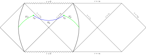
Figure 3: Penrose diagram of Schwarzschild de-Sitter black hole with thermal opaque membrane covering the cosmological patch. The $R_{H}^{\pm}$ regions are shown by green curve with $b_{H}^{\pm}=(\pm t_{b_{H}},b_{H})$. The blue line indicates the complementary region of $R_{H}=R_{H}^{+}\cup R_{H}^{-}$.

The distance $d(b^{+}_{H},b^{-}_{H})$, given in the above expression can be computed explicitly from the metric given in eq.(I). This reads

$$d(b_{H}^{+},b_{H}^{-})=2F(b_{H})e^{\kappa_{H}r^{*}(b_{H})}\cosh(\kappa_{H}t_{b_{H}})\leavevmode\nobreak\ .$$ (32)

Now using the above expression in eq.(31), the entanglement entropy of Hawking radiation is found to be

$$S(R_{H}) = S_{vN}(R^{+}_{H}\cup R^{-}_{H})$$ (33)

$$= \left(\frac{c}{3}\right)\log\left[\left(\frac{\beta_{H}}{\pi}\right)\sqrt{f(b_{H})}\cosh\left(\frac{2\pi t_{b_{H}}}{\beta_{H}}\right)\right].$$

From the above result we can observe that in the early time domain, that is for $t_{b_{H}}\ll\beta_{H}$, the fine grained entropy of Hawking radiation reduces to the following form

$$S(R_{H}) \approx \left(\frac{c}{3}\right)\log\left[\left(\frac{\beta_{H}}{\pi}\right)\sqrt{f(b_{H})}\right]+\left(\frac{c}{6}\right)\left(\frac{2\pi t_{b_{H}}}{\beta_{H}}\right)^{2}\leavevmode\nobreak\ .$$

However, at late times ($t_{b_{H}}\gg\beta_{H}$), we obtain the following form of the entropy of the Haking radiation

$$S(R_{H}) \approx \left(\frac{c}{3}\right)\log\left[\left(\frac{\beta_{H}}{\pi}\right)\sqrt{f(b_{H})}\right]+\left(\frac{c}{3}\right)\left(\frac{2\pi t_{b_{H}}}{\beta_{H}}\right).$$

From the above analysis we observe that as long as there is no island contribution, the entanglement entropy of the Hawking radiation increases with respect to the observer’s time. However, the nature of this time evolution of $S_{vN}(R_{H})$ is strikingly different for these two different time doamins. To be precise, in the early time $S_{vN}(R_{H})$ shows quadratic behaviour with time, that is $S_{vN}(R_{H})\sim t_{b_{H}}^{2}$, and in the late time domain it grows linearly in time, that is $S_{vN}(R_{H})\sim t_{b_{H}}$. This observation firmly agrees with the one shown in Hartman and Maldacena (2013).
One can also compute the entanlement entropy of the matter fields localized on the individual regions $R_{H}^{+}$ and $R_{H}^{-}$. This can be written down as

$$S_{vN}(R_{H}^{\pm}) = \left(\frac{c}{3}\right)\log d(b_{H}^{\pm},e_{H}^{\pm})\leavevmode\nobreak\ .$$ (36)

We can compute the above given distances by using the black hole metric given in eq.(I). The expressions of $d(b_{H}^{+},e_{H}^{+})$ and $d(b_{H}^{-},e_{H}^{-})$ read

$$d(b_{H}^{+},e_{H}^{+}) = \left[2F(b_{H})F(e_{H})e^{\kappa_{H}r^{*}(b_{H})}\left(\cosh(\kappa_{H}r^{*}(b_{H}))-\cosh(\kappa_{H}t_{b_{H}})\right)\right]^{\frac{1}{2}}=d(b_{H}^{-},e_{H}^{-})\leavevmode\nobreak\ .$$ (37)

In the above result we assume that $\mathop{\textrm{Limit}}_{e\rightarrow\infty}r^{*}(e)=0$. By substituting the above expression in eq.(36), we get the following results

$$S_{vN}(R^{+}_{H})=S_{vN}(R^{-}_{H})=\left(\frac{c}{6}\right)\log\left[2\left(\frac{\beta_{H}}{2\pi}\right)^{2}\sqrt{f(b_{H})f(e_{H})}\left\{|\cosh\left(\frac{2\pi r^{*}(b_{H})}{\beta_{H}}\right)-\cosh\left(\frac{2\pi t_{b_{H}}}{\beta_{H}}\right)|\right\}\right]\leavevmode\nobreak\ \leavevmode\nobreak\ \leavevmode\nobreak\ .$$ (38)

Now with the computed results (given in eq.(33) and eq.(38)) in hand one can obtain the expression for the mutual information (MI) between the matter fields localised on the region $R^{+}_{H}$ and $R^{-}_{H}$. This is obtained to be

$$I(R_{H}^{+}:R_{H}^{-}) = S_{vN}(R_{H}^{+})+S_{vN}(R_{H}^{-})-S_{vN}(R_{H}^{+}\cup R_{H}^{-})$$ (39)

$$= \left(\frac{c}{3}\right)\log\left[\left(\frac{\beta_{H}}{2\pi}\right)\sqrt{f(e_{H})}\left\{\frac{|\cosh\left(\frac{2\pi r^{*}(b_{H})}{\beta_{H}}\right)-\cosh\left(\frac{2\pi t_{b_{H}}}{\beta_{H}}\right)|}{\cosh\left(\frac{2\pi t_{b_{H}}}{\beta_{H}}\right)}\right\}\right]\leavevmode\nobreak\ .$$

In order to understand the behaviour of MI thoroughly (for both early and late time scenario), we compute its form by considering the justified limits. In the early time domain $(t_{b_{H}}\ll\beta_{H})$, the expression of mutual information reduces to the following form

$$I(R_{H}^{+}:R_{H}^{-}) \approx \left(\frac{c}{3}\right)\left[\log\left[\left(\frac{\beta_{H}}{2\pi}\right)\sqrt{f(e_{H})}\cosh\left(\frac{2\pi r^{*}(b_{H})}{\beta_{H}}\right)\right]-\mathrm{sech}\left(\frac{2\pi r^{*}(b_{H})}{\beta_{H}}\right)-\left(\frac{2\pi^{2}}{\beta_{H}^{2}}\right)\left\{1+\mathrm{sech}\left(\frac{2\pi r^{*}(b_{H})}{\beta_{H}}\right)\right\}t_{b_{H}}^{2}\right]\leavevmode\nobreak\ .$$

The above expression suggests that at the early time domain $I(R_{H}^{+}:R_{H}^{-})$ decreases with the time-scaling $\sim t_{b_{H}}^{2}$. On the other hand, at the late times ($t_{b_{H}}\gg\beta_{H}$), we obtain the following form of the mutual information

$$I(R_{H}^{+}:R_{H}^{-}) \approx \left(\frac{c}{3}\right)\left[\log\left[\left(\frac{\beta_{H}}{2\pi}\right)\sqrt{f(e_{H})}\right]-2\cosh\left(\frac{2\pi r^{*}(b_{H})}{\beta_{H}}\right)e^{-\left(\frac{2\pi t_{b_{H}}}{\beta_{H}}\right)}\right]\leavevmode\nobreak\ .$$

This in turn means that at late times ($t_{b_{H}}\gg\beta_{H}$), $I(R_{H}^{+}:R_{H}^{-})$ increases with respect to the observer’s time $t_{b_{H}}$. Interestingly, one can note by looking at eq.(s)(II.1) and (II.1) that there exists a particular value of $t_{b_{H}}$ at which the mutual information will be zero and the entanglement wedge corresponding to $R_{H}^{+}\cup R_{H}^{-}$ will be in its disconnected phase. This observation supports the following proposal given in Roy Chowdhury et al. (2022) Proposal I: For an eternal black hole in de-Sitter spacetime, starting from a finite, non-zero value (at $t_{b_{H}}=0$), the mutual information between $R_{H}^{+}$ and $R_{H}^{+}$ vanishes at a particular value of the observer’s time ($t_{b_{H}}=t_{H}$).

Now we will compute the expression of the time scale $t_{H}$ at which the mutual information between $R_{H}^{+}$ and $R_{H}^{-}$ vanishes. In order to do this we will use the expression given in eq.(39) along with the above given proposal. This reads

$$I(R_{H}^{+}:R_{H}^{-})|_{t_{b_{H}}=t_{H}} = 0\leavevmode\nobreak\ .$$ (42)

One can solve the above equation to obtain the value of $t_{H}$. This is found to be

$$t_{H}=\left(\frac{\beta_{H}}{2\pi}\right)\cosh^{-1}\left\{\left(\frac{\frac{\beta_{H}}{2\pi}\sqrt{f(e_{H})}}{1+\frac{\beta_{H}}{2\pi}\sqrt{f(e_{H})}}\right)\cosh\left(\frac{2\pi r^{*}(b_{H})}{\beta_{H}}\right)\right\}.$$

The above expression suggests that the time scale $t_{H}$ is much smaller than $t_{b_{H}}=\beta_{H}$, that is $t_{H}\ll\beta_{H}$. Therefore the time scale $t_{H}$ lies in the early time domain. The expression of $S_{vN}(R_{H}^{+}\cup R_{H}^{-})$ at this particular time ($t_{b_{H}}=t_{H}$) reads

$$S_{vN}^{t_{b_{H}}=t_{H}}(R_{H}^{+}\cup R_{H}^{-}) = \frac{c}{3}\log\left[\frac{\left(\frac{\beta_{H}\sqrt{f(e_{H})}}{2\pi}\right)^{2}}{1+\frac{\beta_{H}\sqrt{f(e_{H})}}{2\pi}}\cosh\left(\frac{2\pi r^{*}(b_{H})}{\beta_{H}}\right)\right]$$

$$\approx \frac{c}{3}\log\left[\frac{\beta_{H}}{2\pi}\sqrt{f(e_{H})}\right]+\frac{c}{6}\left(\frac{r_{H}}{b_{H}}\right)^{2}\leavevmode\nobreak\ .$$

Our proposal suggests that the mutual correlation between $R_{H}^{+}$ and $R_{H}^{-}$ is non-zero for the time interval $0\leq t_{b_{H}}<t_{H}$. The value of $I(R_{+}:R_{-})$ is maximum at $t_{b_{H}}=0$ and then it decreases for the range $t_{b_{H}}\leq t_{H}$, and vanishes exactly at $t_{b_{H}}=t_{H}$. Further, it also depicts the fact that the associated entanglement wedge of $R_{H}^{+}\cup R_{H}^{-}$ is in connected phase initially. Then, at $t_{b_{H}}=t_{H}$, the mutual information between $R_{H}^{+}$ and $R_{H}^{-}$ vanishes and the entanglement wedge associated to $R_{H}^{+}\cup R_{H}^{-}$ makes the transition to the disconnected phase. Once again we would like to mention that $t_{H}\ll\beta_{H}$. These observations strongly indicate that this time $t_{H}$ is nothing but the Hartman-Maldacena time $t_{HM}$, as reported in our previous work Roy Chowdhury et al. (2022). Furthermore, the expression of mutual information, $I(R_{H}^{+}:R_{H}^{-})$ at $t_{b_{H}}=\beta_{H}$ is obtained to be

$$I(R_{H}^{+}:R_{H}^{-}) = \left(\frac{c}{3}\right)\log\left[\left(\frac{\beta_{H}}{2\pi}\right)\sqrt{f(e_{H})}\cosh\left(\frac{2\pi r^{*}(b_{H})}{\beta_{H}}\right)\right]\leavevmode\nobreak\ .$$

The above result tells us that after the Hartman- Maldacena time, the mutual correlation between $R_{H}^{+}$ and $R_{H}^{-}$ ($I(R_{+}:R_{-})$) starts to increase with respect to the observer’s time $t_{b_{H}}$.

II.2 After Page time scenario: probing the role of $I(B_{H}^{+}:B_{H}^{-})$

We now proceed to discuss the after Page time scenario $t_{b_{H}}\geq t_{H}^{Page}$. Just after the Page time $t_{H}^{Page}$, the island starts to contribute. This in turn means that one has to generalize the concept of entanglement entropy by introducing the concept of fine-grained entropy. This generalization incorporates the area term in the formula given in eq.(1) along with the island contribution. One can observe that the term $S_{vN}(I_{H}\cup R_{H})$ satisfies the identity $S_{vN}(I_{H}\cup R_{H}^{+}\cup R_{H}^{-})=S_{vN}(B_{H}^{+}\cup B_{H}^{-})$. The regions of $B_{H}^{\pm}$ can be specified as $(b_{H}^{\pm}\rightarrow a_{H}^{\pm})$ where $a_{H}^{\pm}=(\pm t_{a_{H}},a_{H})$ are the end points of the island. This can be understood by the Penrose diagram, given in Fig(4). Now as we have mentioned earlier, in this work we are considering $2d$ free CFT as the matter sector. This in turn means that the expression associated to $S_{vN}(B_{H}^{+}\cup B_{H}^{-})$ can be evaluated by using the following formula Calabrese et al. (2009)

$$S_{vN}(B_{H}^{+}\cup B_{H}^{-})=\left(\frac{c}{3}\right)\log\Big{[}\frac{d(a_{H}^{+},a_{H}^{-})d(b_{H}^{+},b_{H}^{+})d(a_{H}^{+},b_{H}^{+})d(a_{H}^{-},b_{H}^{-})}{d(a_{H}^{+},b_{H}^{-})d(a_{H}^{-},b_{H}^{+})}\Big{]}\leavevmode\nobreak\ .$$ (46)

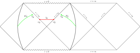
Figure 4: Penrose diagram of the black hole patch (with thermal opaque membrane covering the cosmological patch) indicating the island region (in red) with endpoints $a_{H}^{\pm}=(\pm t_{a_{H}},a_{H})$. The radiation regions are shown by the green line.

Now, in order to compute the explicit form of the entanglement entropy of the matter fields, we have to substitute the distances in eq.(46). This can be calculated from the black hole metric given in eq.(I). In recent works in this direction, it has been suggested that at the late times ($t_{a_{H}},t_{b_{H}}\gg\beta_{H}$), one can make the following approximation Hashimoto et al. (2020); Matsuo (2021)

$$S_{vN}(B_{H}^{+}\cup B_{H}^{-})\approx S_{vN}(B_{H}^{+})+S_{vN}(B_{H}^{-})$$ (47)

where

$$S_{vN}(B_{H}^{\pm})=\left(\frac{c}{3}\right)\log d(b_{H}^{\pm},a_{H}^{\pm})$$ (48)

By using the above mentioned approximation in eq.(1) along with the correct area term and upon extremization one can show that the final expression for $S(R_{H})$ is nothing but $S(R_{H})$, that is $S(R_{H})=2S_{BH}+...$ . This has already been shown in Yadav and Joshi (2023); Krishnan (2021). In Saha et al. (2022); Roy Chowdhury et al. (2022) it was shown that the approximation given in eq.(47) corresponds to the fact that one has to ignore the terms $\sim e^{-\frac{2\pi t_{b_{H}}}{\beta_{H}}}$. This in turn means that the approximation $e^{-\frac{2\pi t_{b_{H}}}{\beta_{H}}}\approx 0$ is associated with the vanishing of mutual information $(I(B_{H}^{+}:B_{H}^{-})=S_{vN}(B_{H}^{+})+S_{vN}(B_{H}^{-})-S_{vN}(B_{H}^{+}\cup B_{H}^{-})\approx 0)$, only at the leading order. However, if the contribution from the terms $\sim e^{-\frac{2\pi t_{b_{H}}}{\beta_{H}}}$ are kept, then it will eventually give us a time-dependent expression of $S(R)$. This issue was addressed in our previous works Saha et al. (2022); Roy Chowdhury et al. (2022). We now extend our previous study for the de-Sitter spacetime by proposing the following Proposal II: For an eternal black hole in de-Sitter spacetime, the mutual information between the black hole subsystems $B_{H}^{+}$ and $B_{H}^{-}$ vanishes just after the Page time when the island starts to contribute. Holographically the above proposal implies that just after the Page time, when the replica wormhole saddle points starts to dominate, the entanglement wedge of $B_{H}^{+}\cup B_{H}^{-}$ makes the transition from connected to disconnected phase Takayanagi and Umemoto (2018); Saha and Gangopadhyay (2021); Chowdhury et al. (2022) and this results in $I(B_{H}^{+}:B_{H}^{-})=0$. Now, according to the above given proposal, we need to compute the following

$$I(B_{H}^{+}:B_{H}^{-}) = 0$$

$$S_{vN}(B_{H}^{+})+S_{vN}(B_{H}^{-}) = S_{vN}(B_{H}^{+}\cup B_{H}^{-})\leavevmode\nobreak\ .$$ (49)

By substituting the explicit expressions from eq.(48) and eq.(46), one obtains the following equality

$$d(a_{H}^{+},b_{H}^{-})(a_{H}^{-},b_{H}^{+}) = d(a_{H}^{+},a_{H}^{-})d(b_{H}^{+},b_{H}^{-})\leavevmode\nobreak\ .$$ (50)

Substituting this equality in $S_{vN}(B^{+}_{H}\cup R^{-}_{H})$ (given in eq.(46)), we obtain

$$S_{vN}(B_{H}^{+}\cup B_{H}^{-})=\frac{c}{3}\log\left(d(a_{H}^{+},b_{H}^{+})d(a_{H}^{-},b_{H}^{-})\right)\leavevmode\nobreak\ .$$ (51)

By using the metric of the black hole patch given in eq.(I), one can compute the explicit expressions corresponding to the mentioned various distances. This reads

$$d(a_{H}^{\pm},b_{H}^{\pm}) = \sqrt{2F(a_{H})F(b_{H})e^{\kappa_{H}(r^{*}(b_{H})+r^{*}(a_{H}))}}\Big{[}\cosh[\kappa_{H}(r^{*}(a_{H})-r^{*}(b_{H}))]-\cosh[\kappa_{H}(t_{a_{H}}-t_{b_{H}})]\Big{]}^{\frac{1}{2}}$$ (52)

$$d(a_{H}^{\pm},b_{H}^{\mp}) = \sqrt{2F(a_{H})F(b_{H})e^{\kappa_{H}(r^{*}(b_{H})+r^{*}(a_{H}))}}\Big{[}\cosh[\kappa_{H}(r^{*}(a_{H})-r^{*}(b_{H}))]+\cosh[\kappa(t_{a_{H}}+t_{b_{H}})]\Big{]}^{\frac{1}{2}}$$ (53)

$$d(b_{H}^{+},b_{H}^{-}) = 2F(b_{H})e^{\kappa_{H}r^{*}(b_{H})}\cosh(\kappa_{H}t_{b_{H}})$$ (54)

$$d(a_{H}^{+},a_{H}^{-}) = 2F(a_{H})e^{\kappa_{H}r^{*}(a_{H})}\cosh(\kappa_{H}t_{a_{H}})\leavevmode\nobreak\ .$$ (55)

These above expressions of distances suggests that

$$d(a^{+}_{H},b^{+}_{H}) = d(a^{-}_{H},b^{-}_{H})$$

$$d(a^{+}_{H},b^{-}_{H}) = d(a^{-}_{H},b^{+}_{H}).$$ (56)

This in turn means that we can recast the expression of $S_{vN}(B^{+}_{H}\cup B^{-}_{H})$ (given in eq.(51)) in the following form

$$S_{vN}(B_{H}^{+}\cup B_{H}^{-})=\frac{2c}{3}\log d(a_{H}^{+},b_{H}^{+})$$ (57)

On the other hand, substituting these expressions of distances in eq.(50) along with fact given in eq.(II.2), we obtain the following condition

$$t_{a_{H}}-t_{b_{H}}=|r^{*}(a_{H})-r^{*}(b_{H})|\leavevmode\nobreak\ .$$ (58)

The above obtained condition is very interesting as it enables us express $t_{a_{H}}$ in terms of the other quantities. By using this mentioned property in eq.(57), we obatin the entanglement entropy of the conformal matter fields

$$S_{vN}(B_{H}^{+}\cup B_{H}^{-})=\frac{c}{3}\log\left(\frac{2}{\kappa_{H}^{2}}\right)+\frac{c}{6}\log[f(a_{H})f(b_{H}))]\leavevmode\nobreak\ .$$

The importance of the above result lies in the fact that it is independent of time. Now if we substitute the above expression in eq.(1) together with the area term, that is $\frac{\mathrm{Area}(\partial I_{H})}{4G_{N}}=2\times\frac{4\pi a_{H}^{2}}{4G_{N}}$, the fine grained entropy of the Hawking radiation reads

$$S(R_{H})=2\times\frac{4\pi a_{H}^{2}}{4G_{N}}+\frac{c}{3}\log\left(\frac{2}{\kappa_{H}^{2}}\right)+\frac{c}{6}\log[f(a_{H})f(b_{H})]\leavevmode\nobreak\ .$$

We now need to find the value of the island parameter ‘$a_{H}$’. This we obtain by performing the extremization of the above result. This leads to the following value

$$a_{H}=r_{H}-\left(\frac{cG_{N}}{24\pi}\right)\frac{1}{r_{H}}+...\leavevmode\nobreak\ .$$ (61)

The above results shows that the quantum extremal surfaces are located inside the black hole event horizon Yadav and Joshi (2023); Goswami and Narayan (2022). However, in case of eternal black holes in AdS, it has been noted that the quantum extremal surfaces reside just outside the event horizon Saha et al. (2022); Roy Chowdhury et al. (2022). So, the position of the island endpoints are different for dS and AdS spacetime. Substitution of the above extremized value of $``a_{H}"$ in eq.(II.2) leads to the following expression of fine-grained entropy of Hawking radiation

$$S(R_{H})=2S_{BH}+\frac{c}{3}\log\left(S_{BH}\right)-\frac{\left(\frac{c}{2}\right)^{2}}{2S_{BH}}+...$$

It can be noted from the above expression that it is time independent and contains logarithmic and inverse power law correction terms Saha et al. (2022); Roy Chowdhury et al. (2022). Revisiting the condition $I(B_{+}:B_{-})=0$ (given in eq.(58)) with the obtained value of $``a_{H}"$ (given in eq.(II.2)), we get

$$t_{a_{H}}-t_{b_{H}}=\left(\frac{\beta_{H}}{8\pi}\right)\log\left(S_{BH}\right)=t_{H}^{Scr}\leavevmode\nobreak\$$ (63)

where $t_{H}^{Scr}$ is the Scrambling timeSekino and Susskind (2008); Hayden and Preskill (2007) for the black hole patch. The remarkable observation made above in turn tells that just after the Page time $t_{H}^{P}$, the replica wormhole saddle points start to dominate and the emergence of island in the black hole interior leads to the disconnected phase of the entanglement wedge $B_{H}^{+}\cup B_{H}^{-}$, characterized by the condition given in eq.(63). On the other hand, the explicit expression of the Page time is found to be

$$t_{H}^{Page}=\left(\frac{3\beta_{H}}{\pi c}\right)S_{BH}-\left(\frac{\beta_{H}}{\pi}\right)\log\left(S_{BH}\right)...\leavevmode\nobreak\ .$$

In the above expression, the leading piece is the familiar form of the Page time, where the rest represent the sub-leading corrections to it.

III Analysis for the cosmological patch

In this part, we will study the Page curve corresponding to the entanglement entropy of Gibbons-Hawking radiation. This we do by restricting ourselves in the cosmological patch and treating the black holes on each side as frozen (for the same reason as in the previous section, we again add two thermal opaque membranes on either side of the black hole patch). For the area of interest, the corresponding metric is given in eq.(I). It has been noted that studies in this direction are often restricted to the black holes in asymptotically flat or AdS spacetimes, however the most recent data shows that the universe is expanding faster with a de-Sitter like characteristics. In this context, the cosmological event horizons emit and absorb radiation similar to the black hole event horizon and this radiation has been denoted as the Gibbons-Hawking radiation. In general, the entropy creation of the cosmic horizon is an observer-dependent feature in contrast to the black hole. It develops as a result of ignorance regarding what exists beyond the cosmological horizon.
Now, in order to study the cosmological patch we have to freeze the black hole patch by the thermal opaque membranes on the both sides. Once again, we will discuss two scenarios here, namely, the before cosmological Page time $(t_{c}^{Page})$ scenario and the after cosmological Page time scenario.

III.1 Before cosmological Page time scenario: The role of $I(R_{c}^{+}:R_{c}^{-})$

Similar to the previous scenario, this time domain corresponds to the facts that the observer’s time is less then the cosmological Page time, that is $t_{c}\ll t_{c}^{Page}$. As mentioned earlier, in this time domain there is no cosmological island contribution. Therefore the entanglement entropy of the Gibbons-Hawking (GH) radiation ($S(R_{c})$) is given by the von Neumann entropy of the matter fields on $R_{c}=R_{c}^{+}\cup R_{c}^{-}$, that is $S(R_{c})=S_{vN}(R_{c})$. It is to be noted that the end points of the disjoint regions $R_{c}^{\pm}$ are $[e_{c}^{\pm}:b_{c}^{\pm}]$. As $R^{\pm}_{c}$ regions are extended to spatial infinity (upto the thermal opaque) from the inner boundary $b^{\pm}_{c}=(\pm t_{b_{c}},b_{c})$, we introduce the point $e^{\pm}_{c}$ in order to regularize it, that is, $e^{\pm}_{c}=(0,e_{c})$. This can be visualised in the Penrose diagram given in Fig.(5). We will eventually take the limit $e_{c}\rightarrow\infty$. Now, we need to compute the following in order to obtain the desired result

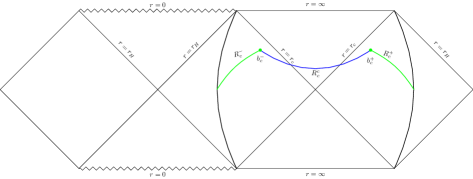
Figure 5: Penrose diagram of cosmological patch of SdS spacetime with thermal opaque. The regions $R_{c}^{\pm}$ is indicated by the green line. The complementary region of $R_{c}=R_{c}^{+}\cup R_{c}^{-}$, that is, $R_{c}^{c}$ is shown by the in figure by blue line.

$$S_{vN}(R_{c}) = S_{vN}(R_{c}^{+}\cup R_{c}^{-})\leavevmode\nobreak\ ;\leavevmode\nobreak\ R_{c}=R^{+}_{c}\cup R^{-}_{c}\leavevmode\nobreak\ .$$ (65)

Once again we assume that the state on the full Cauchy slice is a pure state, therefore the entanglement entropy of the GH radiation reads

$$S_{vN}(R_{c}^{+}\cup R_{c}^{-}) = S_{vN}(R_{c}^{c})$$ (66)

Now, keeping in mind the $s$-wave approximation in the matter sector, we use the $2d$ conformal field theory formula. This reads

$$S_{vN}(R_{c}^{c})=\left(\frac{c}{3}\right)\log d(b^{+}_{c},b^{-}_{c})\leavevmode\nobreak\ .$$ (67)

To compute the distance $d(b^{+}_{c},b^{-}_{c})$, in the cosmological patch we will use the metric given in eq.(I). The in turn gives us

$$d(b_{c}^{+},b_{c}^{-})=2G(b_{c})e^{\kappa_{c}r^{*}(b_{c})}\cosh(\kappa_{c}t_{b_{c}})$$ (68)

where $\kappa_{c}$ (surface gravity of the cosmological patch) is given in eq.(19). The above given result and eq.(67) lead us to the following result for entanglement entropy of the GH radiation

$$S(R_{c}) = S_{vN}(R^{+}_{c}\cup R^{-}_{c})$$ (69)

$$= \left(\frac{c}{3}\right)\log\left[\left(\frac{\beta_{c}}{\pi}\right)\sqrt{f(b_{c})}\cosh\left(\frac{2\pi t_{b_{c}}}{\beta_{c}}\right)\right].$$

We now follow the footstep shown in the previous section and compute the form of $S(R_{c})$ for both early and late time domains. In the early time domain ($t_{b_{c}}\ll\beta_{c}$), $S(R_{c})$ reduces to the following form

$$S(R_{c}) \approx \left(\frac{c}{3}\right)\log\left[\left(\frac{\beta_{c}}{\pi}\right)\sqrt{f(b_{c})}\right]+\left(\frac{c}{6}\right)\left(\frac{2\pi t_{b_{c}}}{\beta_{c}}\right)^{2}\leavevmode\nobreak\ .$$

On the other hand, in late time domain ($t_{c}^{Page}>t_{b_{c}}\gg\beta_{c}$), it reads

$$S(R_{c}) \approx \left(\frac{c}{3}\right)\log\left[\left(\frac{\beta_{c}}{\pi}\right)\sqrt{f(b_{c})}\right]+\left(\frac{c}{3}\right)\left(\frac{2\pi t_{b_{c}}}{\beta_{c}}\right).$$

Once again we note that, in absence of the island contribution, $S(R_{c})$ exhibits quadratic behaviour over time in the early time domain $S(R_{c})\sim t_{b_{c}}^{2}$ and linearly with time for the late time domain $S_{vN}(R_{c})\sim t_{b_{c}}$. Further, the entanglement entropy of the matter fields localized on the individual areas $R_{c}^{+}$ and $R_{c}^{-}$ are obtained to be

$$S_{vN}(R^{\pm}_{c})=\frac{c}{3}\log d(b^{\pm}_{c},e^{\pm}_{c})$$ (72)

Using the metric on the cosmological patch provided in eq.(I), we can calculate the distances. The expressions of $d(b_{c}^{+},e_{c}^{+})$ and $d(b_{c}^{-},e_{c}^{-})$ read

$$d(b_{c}^{+},e_{c}^{+}) = \left[2G(b_{c})G(e_{c})e^{\kappa_{c}r^{*}(b_{c})}\left(\cosh(\kappa_{c}r^{*}(b_{c}))-\cosh(\kappa_{c}t_{b_{c}})\right)\right]^{\frac{1}{2}}=d(b_{c}^{-},e_{c}^{-})\leavevmode\nobreak\ .$$ (73)

In the above expression we are using the fact that, in the limit $e_{c}\rightarrow\infty$, $r^{*}(e)$ vanishes. By replacing the aforementioned formula in the eq.(72), we get the following results

$$S_{vN}(R_{c}^{+})=S_{vN}(R_{c}^{-})=\left(\frac{c}{6}\right)\log\left[2\left(\frac{\beta_{c}}{2\pi}\right)^{2}\sqrt{f(b_{c})f(e_{c})}\left\{|\cosh\left(\frac{2\pi r^{*}(b_{c})}{\beta_{c}}\right)-\cosh\left(\frac{2\pi t_{b_{c}}}{\beta_{c}}\right)|\right\}\right]\leavevmode\nobreak\ .$$ (74)

Now, by using the expressions provided in eq.(69) and eq.(74), we once again compute the mutual information between $R_{c}^{+}$ and $R_{c}^{-}$. This reads

$$I(R_{c}^{+}:R_{c}^{-}) = S_{vN}(R_{c}^{+})+S_{vN}(R_{c}^{-})-S_{vN}(R_{c}^{+}\cup R_{c}^{-})$$

$$= \left(\frac{c}{3}\right)\log\left[\left(\frac{\beta_{c}}{2\pi}\right)\sqrt{f(e_{c})}\left\{\frac{|\cosh\left(\frac{2\pi r^{*}(b_{c})}{\beta_{c}}\right)-\cosh\left(\frac{2\pi t_{b_{c}}}{\beta_{c}}\right)|}{\cosh\left(\frac{2\pi t_{b_{c}}}{\beta_{c}}\right)}\right\}\right]\leavevmode\nobreak\ .$$

Similar to the black hole patch analysis, one can show that in the early time domain $I(R_{c}^{+}:R_{c}^{-})$ decreases with the time-scaling $\sim t_{b_{c}}^{2}$ and for the late time domain ($t_{b_{c}}\gg\beta_{c}$), $I(R_{c}^{+}:R_{c}^{-})$ increases with respect to the observer’s time $t_{b_{c}}$. This once again points out the fact that there exits a time $t_{c}$, at which mutual information between $R_{c}^{+}$ and $R_{c}^{-}$ vanishes and the entanglement wedge associated to $R_{c}^{+}\cup R_{c}^{-}$ gets disconnected. Keeping this in mind, it can be said that the following proposal is valid also for the cosmological patch Proposal I: For an eternal black hole in de-Sitter spacetime, starting from a finite, non-zero value (at $t_{b_{c}}=0$), the mutual information between $R_{c}^{+}$ and $R_{c}^{+}$ vanishes at a particular value of the observer’s time ($t_{b_{c}}=t_{c}$).

In this case, the value of the time-scale $t_{c}$ is obtained to be

$$t_{c}=\left(\frac{\beta_{c}}{2\pi}\right)\cosh^{-1}\left\{\left(\frac{\frac{\beta_{c}}{2\pi}\sqrt{f(e_{c})}}{1+\frac{\beta_{c}}{2\pi}\sqrt{f(e_{c})}}\right)\cosh\left(\frac{2\pi r^{*}(b_{c})}{\beta_{c}}\right)\right\}.$$

Once again we note that the time scale $t_{c}$ is substantially lower than $t_{b_{c}}=\beta_{c}$, that is $t_{c}\ll\beta_{c}$. As a result, the time scale $t_{c}$ belongs to the early time domain. Furthermore, the expression of $S_{vN}(R_{c}^{+}\cup R_{c}^{-})$ at this particular time reads

$$S_{vN}^{t_{b_{c}}=t_{c}}(R_{c}^{+}\cup R_{c}^{-}) = \frac{c}{3}\log\left[\frac{\left(\frac{\beta_{c}\sqrt{f(e_{c})}}{2\pi}\right)^{2}}{1+\frac{\beta_{c}\sqrt{f(e_{c})}}{2\pi}}\cosh\left(\frac{2\pi r^{*}(b_{c})}{\beta_{c}}\right)\right]$$ (77)

$$\approx \frac{c}{3}\log\left[\frac{\beta_{c}}{2\pi}\sqrt{f(e_{c})}\right]+\frac{c}{6}\left(\frac{r_{c}}{b_{c}}\right)^{2}\leavevmode\nobreak\ .$$

This in turn means that for the cosmological patch also the mutual correlation between $R_{c}^{+}$ and $R_{c}^{-}$ is non-zero for the time period $0\leq t_{b_{c}}<t_{c}$ and it reaches its maximum value at $t_{b_{c}}=0$. After that $I(R_{c}^{+}:R_{c}^{-})$ decreases for the range $t_{b_{c}}\leq t_{c}$ and finally disappears at $t_{b_{c}}=t_{c}$. This also reflects the fact that the connected phase of the corresponding entanglement wedge of $R_{c}^{+}\cup R_{c}^{-}$ gets disconnected at $t_{b_{c}}=t_{c}$. These findings once again clearly suggest that $t_{c}$ is the Hartman-Maldacena time for the cosmological patch. After this time (Hartman-Maldacena time) the mutual information between $R_{c}^{+}$ and $R_{c}^{-}$ increases with respect to the observer’s time.

III.2 After Cosmological Page time scenario: The role of $I(B_{c}^{+}:B_{c}^{-})$

Now, once again we proceed to probe the after cosmological Page time scenario. As we have mentioned earlier, Just after the cosmological Page time ($t_{c}^{Page}$) the island starts contribute to the fine grained entropy of Gibbons-Hawking radiation.

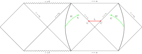
Figure 6: The above Penrose diagram shows the cosmological patch with the thermal opaque membrane. The red line indicates the cosmological island surface with end points $a_{c}^{\pm}=[\pm t_{a_{c}},a_{c}]$. The green lines indicate the radiation regions.

Using the fact that the matter part of eq.(1) satisfies the property $S_{vN}(I_{c}\cup R_{c}^{+}\cup R_{c}^{-})=S_{vN}(B_{c}^{+}\cup B_{c}^{-})$. The regions of $B_{c}^{\pm}$ can be specified as $(b_{c}^{\pm}\rightarrow a_{c}^{\pm})$, where the island end points are pointed out as $a_{c}^{\pm}=(\pm t_{a_{c}},a_{c})$. The Penrose diagram given in Fig.(6) helps us to visualise this. We now follow the steps shown in the black hole patch scenario. As we have already stated, the matter sector in this work is the $2d$ free CFT. As a result, the expression of $S_{vN}(B_{c}^{+}\cup B_{c}^{-})$ can be evaluated using the following formula Calabrese et al. (2009)

$$S_{vN}(B_{c}^{+}\cup B_{c}^{-})=\left(\frac{c}{3}\right)\log\Big{[}\frac{d(a_{c}^{+},a_{c}^{-})d(b_{c}^{+},b_{c}^{-})d(a_{c}^{+},b_{c}^{+})d(a_{c}^{-},b_{c}^{-})}{d(a_{c}^{+},b_{c}^{-})d(a_{c}^{-},b_{c}^{+})}\Big{]}\leavevmode\nobreak\$$

The distances that may be derived from the metric provided in eq.(I) must be replaced in in the above expression in order to obtain the explicit form of the entanglement entropy of the matter field. The entropy of the matter field on the individual regions can be computed by the following expression

$$S_{vN}(B_{c}^{\pm}) = \left(\frac{c}{3}\right)\log d(b_{c}^{\pm},a_{c}^{\pm})\leavevmode\nobreak\ .$$ (79)

Now, as we have already mentioned for the black hole patch analysis, one can compute $S_{vN}(B_{c}^{+}\cup B_{c}^{-})$ for late time by using the following approximation

$$S_{vN}(B_{c}^{+}\cup B_{c}^{-})\sim S_{vN}(B_{c}^{+})+S_{vN}(B_{c}^{-})\leavevmode\nobreak\ .$$ (80)

The above mentioned approximation is once again associated to the fact that one has to neglect the terms $\sim e^{-\frac{2\pi t_{b_{c}}}{\beta_{c}}}$ which provides the indication of vanishing mutual correlation (only in the leading order) between $B_{c}^{+}$ and $B_{c}^{-}$. This observation is similar to the one we have already noted for the black hole patch scenario which in turn means that the following proposal should also hold for the cosmological patch Proposal II: For an eternal black hole in de-Sitter spacetime, the mutual information between the between the matter fields localised on $B_{c}^{+}$ and $B_{c}^{-}$ vanishes just after the cosmological Page time. By following the same procedure we have already shown for the black hole patch, one can obtain the time-independent form of fine-grained entropy of GH radiation by using the above given proposal. This reads

$$S(R_{c})=2\times\frac{4\pi a_{c}^{2}}{4G_{N}}+\frac{c}{3}\log\left(\frac{2}{\kappa_{c}^{2}}\right)+\frac{c}{6}\log[f(a_{c})f(b_{c})]\leavevmode\nobreak\ .$$

Extremising the above result with respect to the cosmological island parameter “$a_{c}$”, we get

$$a_{c}=r_{c}-\left(\frac{cG_{N}}{24\pi}\right)\frac{1}{r_{c}}+...\leavevmode\nobreak\ .$$ (82)

The above result indicates that the cosmological island end points (quantum extremal surfaces) are located inside the cosmological horizon Yadav and Joshi (2023). By using the result given in eq.(82), we obtain the desired result of fine grained entropy of Gibbons-Hawking radiation

$$S(R_{c})=2S_{GH}+\frac{c}{3}\log\left(S_{GH}\right)-\frac{\left(\frac{c}{2}\right)^{2}}{2S_{GH}}+...\leavevmode\nobreak\ .$$ (83)

Furthermore, the extremized value of the cosmological island parameter simplifies condition of vanishing mutual information to the following form

$$t_{a_{c}}-t_{b_{c}}=\left(\frac{\beta_{c}}{8\pi}\right)\log\left(S_{GH}\right)=t_{c}^{Scr}\leavevmode\nobreak\ .$$ (84)

where $t_{c}^{Scr}$ scrambling time for the cosmological patch. Further the expressionof the cosmological Page time is obtained to be Yadav and Joshi (2023)

$$t_{c}^{P}\approx\left(\frac{3\beta_{c}}{\pi c}\right)S_{GH}\leavevmode\nobreak\ .$$ (85)

IV Conclusions

We now provide a summary of our findings. In this work, we have tried to check whether our previously reported proposals Saha et al. (2022); Roy Chowdhury et al. (2022) holds for eternal black holes in de-Sitter spacetime or not. The said proposals were originally given for eternal black holes in AdS spacetime and in this work we have observed that the mentioned proposals also holds for eternal black holes in de-Sitter spacetime. The motivation to consider an eternal black hole solution in de-Sitter spacetime is associated to the subtle structure of the event-horizon for this spacetime. We have briefly investigated the role of mutual information of various subsystems in the Page curve for both Hawking radiation and Gibbons-Hawking radiation, by keeping in mind the recent developments of the island formulation. In order to study the Page curve of above mentioned two different radiations, we have introduced the notion of thermal opaque membrane. This membrane allows us to study the two different radiations individually as it divides the whole system into two patches (equivalent descriptions), namely, the black hole patch and the cosmological patch. Further, the findings from the study of mutual information have motivated us to give two proposals for both the Black hole patch and the cosmological patch of the Schwarzschild de-Sitter spacetime.
The first proposal deals with the time domain where the observer’s time is less than the Page time. First, we will discuss the importance of this proposal for the black hole patch. In this time domain the entanglement entropy of Hawking radiation does not include the island contribution. The entropy of the radiation is identified as the von-Neumann entropy of the conformal matter fields on $R_{H}^{+}\cup R_{H}^{-}$. We have incorporated the formula of $2d$ CFT in order to calculate the mentioned von Neumann entropy $S_{vN}(R_{H})=S_{vN}(R_{H}^{+}\cup R_{H}^{-})$ as we have stated that we are only considering the $s$-wave contribution of the conformal matter. In the early time domain, that is for $t_{b_{H}}\ll\beta_{H}$, we note that $S(R_{H})$ shows quadratic growth ($S(R_{H})\sim t_{b_{H}}^{2}$) and in the late time domain ($t_{b_{H}}\gg\beta_{H}$) $S(R_{H})$ increases linearly with respect to the observer’s time ($S(R_{H})\sim t_{b_{H}}$). The mutual information $I(R_{H}^{+}:R_{H}^{-})$ between $R_{H}^{+}$ and $R_{H}^{-}$ is then computed by obtaining the explicit expressions of $S_{vN}(R_{H}^{+})$ and $S_{vN}(R_{H}^{-})$. With the general expression of $I(R_{H}^{+}:R_{H}^{-})$ in hand, we then proceed to investigate its behaviour in both the early and late time domain. In the early time domain, starting from the maximum value at $t_{b_{H}}=0$, $I(R_{H}^{+}:R_{H}^{-})$ starts decreasing with the time-scaling $\sim t_{b_{H}}^{2}$ and in the late time domain we find that $I(R_{H}^{+}:R_{H}^{-})$ increases with respect to $t_{b_{H}}$. This kind behaviour of the mutual information motivates us to give our first proposal which tells us that there exits a time, $t_{b_{H}}=t_{H}$ ($0<t_{H}<\beta_{H}$) at which the mutual correlation between $R_{H}^{+}$ and $R_{H}^{-}$ disappears. This in turn implies that the associated entanglement wedge $R_{H}^{+}\cup R_{H}^{-}$ becomes disconnected. Further, at $t_{b_{H}}=t_{H}$, the entropy of Hawking radiation is proportional to the logarithm of the inverse temperature of the black hole, that is $S(R_{H})|_{t_{b_{H}}=t_{H}}\sim\log\beta_{H}$. These observations indicates that this particular time-scale $t_{H}$ is nothing but the Hartman-Maldacena time for the black hole patch. After $t_{b_{H}}=t_{H}$, $I(R_{H}^{+}:R_{H}^{-})$ starts to increase, which in turns means that the associated entanglement wedge is once again in its connected phase. In the case of cosmological patch also we have observed similar kind of phenomena before the cosmological “Page time” $t^{Page}_{c}$ and the Hartman-Maldacena time for the cosmological patch is denoted as $t_{c}$. The explicit expressions corresponding to both $t_{H}$ and $t_{c}$ has also been computed.
Now we will discuss about our second proposal. This proposal is associated to the time domain where the observer’s time is greater than the Page time. In case of the black hole patch, after the Page time $(t_{H}^{Page})$, the entropy of Hawking radiation includes the island contribution. This inclusion of island contribution provides appropriate Page curve which portrays the time evolution of the entropy of the Hawking radiation. Following the works in this direction, it has been noted that to obtain the correct Page curve we have to use the late time approximation $S_{vN}(B_{H}^{+}\cup B_{H}^{-})\approx S_{vN}(B_{H}^{+})+S_{vN}(B_{H}^{-})$ Hashimoto et al. (2020) which can also be understood as $I(B_{H}^{+}:B_{H}^{-})$ but only at the leading order. This approximation is associated to the fact that one has to ignore terms $\sim e^{-\frac{2\pi t_{b_{H}}}{\beta_{H}}}$. This creates a dilemma as the the core issue in this context is regarding time-dependency. However, if these terms are incorporated one gets a time-dependent form of $S(R)$ in the after Page time scenario. We address this crucial issue by demanding that the inclusion of island (replica wormhole saddle-point contributions) leads to the disconnected phase of the entanglement wedge associated to $B_{H}^{+}\cup B_{H}^{-}$. This in turns means that just after the Page time $(t_{H}^{P})$, island in turn gifts us the vanishing mutual information between $B_{H}^{+}$ and $B_{H}^{-}$. This condition of vanishing mutual information, that is $I(B_{H}^{+}:B_{H}^{-})=0$ leads to the remarkable result $t_{a_{H}}-t_{b_{H}}=t_{H}^{Scr}$ where $t_{H}^{Scr}$ is the scrambling time Sekino and Susskind (2008); Hayden and Preskill (2007). Using the subadditivity condition of von Neumann entropy we can reforge our observation in the following way. The entanglement wedge associated to $B_{H}^{+}\cup B_{H}^{+}$ is in connected phase as long as $t_{a_{H}}-t_{b_{H}}<t_{H}^{Scr}$, and when this time difference equals the scrambling time $t_{H}^{Scr}$, the entanglement wedge associated to $B_{H}^{+}\cup B_{H}^{+}$ jumps to the disconnected phase. Most importantly this condition of vanishing mutual information condition gives us the time-independent expression of the entropy of the Hawking radiation. Our proposals and observations related to mutual information gives strong realization of the concept given in Grimaldi et al. (2022); Van Raamsdonk (2010). For the cosmological patch also our second proposal implies that after the cosmological Page time when the island statrs contributes the entanglement wedge associated to $B_{c}^{+}\cup B_{c}^{-}$ is in the disconnected phase. Our proposal also implies that for the cosmological patch we have $t_{a_{c}}-t_{b_{c}}=t_{c}^{Scr}$, with $t_{c}^{Scr}$ is the Scrambling time for the cosmological patch. Similar to the black hole patch scenario, we also obtain a time independent result of the entropy of the Gibbons-Haking entropy by imposing the condition of vanishing mutual information between $B_{c}^{+}$ and $B_{c}^{-}$. Another interesting fact to point out is that in both of the cases the quantum extremal surfaces lie inside the respective horizons. This behaviour is opposite to the one we observe for the eternal black hole in AdS spacetime.

V Acknowledgements

ARC would like to thank SNBNCBS for Senior Research Fellowship. AS would like to acknowledge the support by Council of Scientific and Industrial Research (CSIR, Govt. of India) for the Senior Research Fellowship. The authors would like to thank the anonymous referee for very useful comments.

References

- Hawking (1975) S. W. Hawking, “Particle Creation by Black Holes,” Commun. Math. Phys. 43, 199–220 (1975), [Erratum: Commun.Math.Phys. 46, 206 (1976)].
- Nielsen and Chuang (2000) Michael A. Nielsen and Isaac L. Chuang, Quantum Computation and Quantum Information (Cambridge University Press, 2000).
- Hawking (1976a) S. W. Hawking, “Breakdown of predictability in gravitational collapse,” Phys. Rev. D 14, 2460–2473 (1976a).
- Bekenstein (1972) J. D. Bekenstein, “Black holes and the second law,” Lett. Nuovo Cim. 4, 737–740 (1972).
- Bekenstein (1973) Jacob D. Bekenstein, “Black holes and entropy,” Phys. Rev. D 7, 2333–2346 (1973).
- Hawking (1976b) S. W. Hawking, “Black holes and thermodynamics,” Phys. Rev. D 13, 191–197 (1976b).
- Page (1993) Don N. Page, “Information in black hole radiation,” Phys. Rev. Lett. 71, 3743–3746 (1993).
- Page (2013) Don N Page, “Time dependence of hawking radiation entropy,” Journal of Cosmology and Astroparticle Physics 2013, 028–028 (2013).
- Almheiri et al. (2013a) Ahmed Almheiri, Donald Marolf, Joseph Polchinski, and James Sully, “Black Holes: Complementarity or Firewalls?” JHEP 02, 062 (2013a), arXiv:1207.3123 [hep-th] .
- Almheiri et al. (2013b) Ahmed Almheiri, Donald Marolf, Joseph Polchinski, Douglas Stanford, and James Sully, “An Apologia for Firewalls,” JHEP 09, 018 (2013b), arXiv:1304.6483 [hep-th] .
- Lloyd and Preskill (2014) Seth Lloyd and John Preskill, “Unitarity of black hole evaporation in final-state projection models,” JHEP 08, 126 (2014), arXiv:1308.4209 [hep-th] .
- Papadodimas and Raju (2014) Kyriakos Papadodimas and Suvrat Raju, “Black Hole Interior in the Holographic Correspondence and the Information Paradox,” Phys. Rev. Lett. 112, 051301 (2014), arXiv:1310.6334 [hep-th] .
- Penington (2020) Geoffrey Penington, “Entanglement Wedge Reconstruction and the Information Paradox,” JHEP 09, 002 (2020), arXiv:1905.08255 [hep-th] .
- Almheiri et al. (2019a) Ahmed Almheiri, Netta Engelhardt, Donald Marolf, and Henry Maxfield, “The entropy of bulk quantum fields and the entanglement wedge of an evaporating black hole,” JHEP 12, 063 (2019a), arXiv:1905.08762 [hep-th] .
- Almheiri et al. (2020a) Ahmed Almheiri, Raghu Mahajan, Juan Maldacena, and Ying Zhao, “The Page curve of Hawking radiation from semiclassical geometry,” JHEP 03, 149 (2020a), arXiv:1908.10996 [hep-th] .
- Almheiri et al. (2019b) Ahmed Almheiri, Raghu Mahajan, and Juan Maldacena, “Islands outside the horizon,” (2019b), arXiv:1910.11077 [hep-th] .
- Engelhardt and Wall (2015) Netta Engelhardt and Aron C. Wall, “Quantum Extremal Surfaces: Holographic Entanglement Entropy beyond the Classical Regime,” JHEP 01, 073 (2015), arXiv:1408.3203 [hep-th] .
- Engelhardt and Fischetti (2019) Netta Engelhardt and Sebastian Fischetti, “Surface Theory: the Classical, the Quantum, and the Holographic,” Class. Quant. Grav. 36, 205002 (2019), arXiv:1904.08423 [hep-th] .
- Akers et al. (2020) Chris Akers, Netta Engelhardt, Geoff Penington, and Mykhaylo Usatyuk, “Quantum Maximin Surfaces,” JHEP 08, 140 (2020), arXiv:1912.02799 [hep-th] .
- Wall (2014) Aron C. Wall, “Maximin Surfaces, and the Strong Subadditivity of the Covariant Holographic Entanglement Entropy,” Class. Quant. Grav. 31, 225007 (2014), arXiv:1211.3494 [hep-th] .
- Ryu and Takayanagi (2006) Shinsei Ryu and Tadashi Takayanagi, “Holographic derivation of entanglement entropy from the anti–de sitter space/conformal field theory correspondence,” Phys. Rev. Lett. 96, 181602 (2006).
- Hubeny et al. (2007) Veronika E. Hubeny, Mukund Rangamani, and Tadashi Takayanagi, “A Covariant holographic entanglement entropy proposal,” JHEP 07, 062 (2007), arXiv:0705.0016 [hep-th] .
- Almheiri et al. (2020b) Ahmed Almheiri, Thomas Hartman, Juan Maldacena, Edgar Shaghoulian, and Amirhossein Tajdini, “Replica Wormholes and the Entropy of Hawking Radiation,” JHEP 05, 013 (2020b), arXiv:1911.12333 [hep-th] .
- Penington et al. (2022) Geoff Penington, Stephen H. Shenker, Douglas Stanford, and Zhenbin Yang, “Replica wormholes and the black hole interior,” JHEP 03, 205 (2022), arXiv:1911.11977 [hep-th] .
- Goto et al. (2021) Kanato Goto, Thomas Hartman, and Amirhossein Tajdini, “Replica wormholes for an evaporating 2D black hole,” JHEP 04, 289 (2021), arXiv:2011.09043 [hep-th] .
- Colin-Ellerin et al. (2021) Sean Colin-Ellerin, Xi Dong, Donald Marolf, Mukund Rangamani, and Zhencheng Wang, “Real-time gravitational replicas: Formalism and a variational principle,” JHEP 05, 117 (2021), arXiv:2012.00828 [hep-th] .
- Almheiri et al. (2021) Ahmed Almheiri, Thomas Hartman, Juan Maldacena, Edgar Shaghoulian, and Amirhossein Tajdini, “The entropy of Hawking radiation,” Rev. Mod. Phys. 93, 035002 (2021), arXiv:2006.06872 [hep-th] .
- Chen et al. (2020) Hong Zhe Chen, Zachary Fisher, Juan Hernandez, Robert C Myers, and Shan-Ming Ruan, “Information flow in black hole evaporation,” Journal of High Energy Physics 2020, 1–49 (2020).
- Hashimoto et al. (2020) Koji Hashimoto, Norihiro Iizuka, and Yoshinori Matsuo, “Islands in Schwarzschild black holes,” JHEP 06, 085 (2020), arXiv:2004.05863 [hep-th] .
- Hartman et al. (2020) Thomas Hartman, Edgar Shaghoulian, and Andrew Strominger, “Islands in Asymptotically Flat 2D Gravity,” JHEP 07, 022 (2020), arXiv:2004.13857 [hep-th] .
- Anegawa and Iizuka (2020) Takanori Anegawa and Norihiro Iizuka, “Notes on islands in asymptotically flat 2d dilaton black holes,” JHEP 07, 036 (2020), arXiv:2004.01601 [hep-th] .
- Dong et al. (2020) Xi Dong, Xiao-Liang Qi, Zhou Shangnan, and Zhenbin Yang, “Effective entropy of quantum fields coupled with gravity,” JHEP 10, 052 (2020), arXiv:2007.02987 [hep-th] .
- Balasubramanian et al. (2021) Vijay Balasubramanian, Arjun Kar, and Tomonori Ugajin, “Islands in de Sitter space,” JHEP 02, 072 (2021), arXiv:2008.05275 [hep-th] .
- Raju (2022a) Suvrat Raju, “Lessons from the information paradox,” Phys. Rept. 943, 1–80 (2022a), arXiv:2012.05770 [hep-th] .
- Alishahiha et al. (2021) Mohsen Alishahiha, Amin Faraji Astaneh, and Ali Naseh, “Island in the presence of higher derivative terms,” JHEP 02, 035 (2021), arXiv:2005.08715 [hep-th] .
- Krishnan (2021) Chethan Krishnan, “Critical Islands,” JHEP 01, 179 (2021), arXiv:2007.06551 [hep-th] .
- Krishnan et al. (2020) Chethan Krishnan, Vaishnavi Patil, and Jude Pereira, “Page Curve and the Information Paradox in Flat Space,” (2020), arXiv:2005.02993 [hep-th] .
- Azarnia et al. (2021) Sanam Azarnia, Reza Fareghbal, Ali Naseh, and Hamed Zolfi, “Islands in flat-space cosmology,” Phys. Rev. D 104, 126017 (2021), arXiv:2109.04795 [hep-th] .
- Yu and Ge (2022a) Ming-Hui Yu and Xian-Hui Ge, “Islands and Page curves in charged dilaton black holes,” Eur. Phys. J. C 82, 14 (2022a), arXiv:2107.03031 [hep-th] .
- Aref’eva and Volovich (2021) Irina Aref’eva and Igor Volovich, “A Note on Islands in Schwarzschild Black Holes,” (2021), arXiv:2110.04233 [hep-th] .
- He et al. (2022) Song He, Yuan Sun, Long Zhao, and Yu-Xuan Zhang, “The universality of islands outside the horizon,” JHEP 05, 047 (2022), arXiv:2110.07598 [hep-th] .
- Omidi (2022) Farzad Omidi, “Entropy of Hawking radiation for two-sided hyperscaling violating black branes,” JHEP 04, 022 (2022), arXiv:2112.05890 [hep-th] .
- Yu et al. (2022) Ming-Hui Yu, Cheng-Yuan Lu, Xian-Hui Ge, and Sang-Jin Sin, “Island, Page curve, and superradiance of rotating BTZ black holes,” Phys. Rev. D 105, 066009 (2022), arXiv:2112.14361 [hep-th] .
- Ahn et al. (2022) Byoungjoon Ahn, Sang-Eon Bak, Hyun-Sik Jeong, Keun-Young Kim, and Ya-Wen Sun, “Islands in charged linear dilaton black holes,” Phys. Rev. D 105, 046012 (2022), arXiv:2107.07444 [hep-th] .
- Yadav (2022) Gopal Yadav, “Page Curves of Reissner-Nordström Black Hole in HD Gravity,” (2022), arXiv:2204.11882 [hep-th] .
- Du et al. (2022) Dong-Hui Du, Wen-Cong Gan, Fu-Wen Shu, and Jia-Rui Sun, “Unitary Constraints on Semiclassical Schwarzschild Black Holes in the Presence of Island,” (2022), arXiv:2206.10339 [hep-th] .
- Hosseini Mansoori et al. (2022) Seyed Ali Hosseini Mansoori, Orlando Luongo, Stefano Mancini, Mirmani Mirjalali, Morteza Rafiee, and Alireza Tavanfar, “Planar black holes in holographic axion gravity: Islands, Page times, and scrambling times,” Phys. Rev. D 106, 126018 (2022), arXiv:2209.00253 [hep-th] .
- Ageev et al. (2022) D. S. Ageev, I. Ya. Aref’eva, A. I. Belokon, A. V. Ermakov, V. V. Pushkarev, and T. A. Rusalev, “Entanglement Islands and Infrared Anomalies in Schwarzschild Black Hole,” (2022), arXiv:2209.00036 [hep-th] .
- Yu and Ge (2022b) Ming-Hui Yu and Xian-Hui Ge, “Entanglement Islands in Generalized Two-dimensional Dilaton Black Holes,” (2022b), arXiv:2208.01943 [hep-th] .
- Hu et al. (2022a) Peng-Ju Hu, Dongqi Li, and Rong-Xin Miao, “Island on codimension-two branes in AdS/dCFT,” JHEP 11, 008 (2022a), arXiv:2208.11982 [hep-th] .
- Takayanagi (2011) Tadashi Takayanagi, “Holographic dual of a boundary conformal field theory,” Physical review letters 107, 101602 (2011).
- Fujita et al. (2011) Mitsutoshi Fujita, Tadashi Takayanagi, and Erik Tonni, “Aspects of ads/bcft,” Journal of High Energy Physics 2011, 1–40 (2011).
- Nozaki et al. (2012) Masahiro Nozaki, Tadashi Takayanagi, and Tomonori Ugajin, “Central charges for bcfts and holography,” Journal of High Energy Physics 2012, 1–25 (2012).
- Miao et al. (2017) Rong-Xin Miao, Chong-Sun Chu, and Wu-Zhong Guo, “New proposal for a holographic boundary conformal field theory,” Phys. Rev. D 96, 046005 (2017).
- Geng and Karch (2020) Hao Geng and Andreas Karch, “Massive islands,” JHEP 09, 121 (2020), arXiv:2006.02438 [hep-th] .
- Geng et al. (2021a) Hao Geng, Yasunori Nomura, and Hao-Yu Sun, “Information paradox and its resolution in de Sitter holography,” Phys. Rev. D 103, 126004 (2021a), arXiv:2103.07477 [hep-th] .
- Geng et al. (2021b) Hao Geng, Severin Lüst, Rashmish K. Mishra, and David Wakeham, “Holographic BCFTs and Communicating Black Holes,” jhep 08, 003 (2021b), arXiv:2104.07039 [hep-th] .
- Hu et al. (2022b) Qi-Lin Hu, Dongqi Li, Rong-Xin Miao, and Yu-Qian Zeng, “Ads/bcft and island for curvature-squared gravity,” Journal of High Energy Physics 2022, 1–46 (2022b).
- Geng et al. (2022a) Hao Geng, Andreas Karch, Carlos Perez-Pardavila, Suvrat Raju, Lisa Randall, Marcos Riojas, and Sanjit Shashi, “Entanglement phase structure of a holographic BCFT in a black hole background,” JHEP 05, 153 (2022a), arXiv:2112.09132 [hep-th] .
- Rozali et al. (2020) Moshe Rozali, James Sully, Mark Van Raamsdonk, Christopher Waddell, and David Wakeham, “Information radiation in bcft models of black holes,” Journal of High Energy Physics 2020, 1–34 (2020).
- Almheiri et al. (2020c) Ahmed Almheiri, Raghu Mahajan, and Jorge Santos, “Entanglement islands in higher dimensions,” SciPost Physics 9, 001 (2020c).
- Bousso and Wildenhain (2020) Raphael Bousso and Elizabeth Wildenhain, “Gravity/ensemble duality,” Physical Review D 102, 066005 (2020).
- Afrasiar et al. (2023) Mir Afrasiar, Jaydeep Kumar Basak, Ashish Chandra, and Gautam Sengupta, “Reflected Entropy for Communicating Black Holes II: Planck Braneworlds,” (2023), arXiv:2302.12810 [hep-th] .
- Afrasiar et al. (2022) Mir Afrasiar, Jaydeep Kumar Basak, Ashish Chandra, and Gautam Sengupta, “Islands for Entanglement Negativity in Communicating Black Holes,” (2022), arXiv:2205.07903 [hep-th] .
- Guo et al. (2023) Chang-Zhong Guo, Wen-Cong Gan, and Fu-Wen Shu, “Page curves and Entanglement Islands for the Step-Function Vaidya Model of Evaporating Black Holes,” (2023), arXiv:2302.02379 [hep-th] .
- Miao (2023) Rong-Xin Miao, “Entanglement Island and Page Curve in Wedge Holography,” (2023), arXiv:2301.06285 [hep-th] .
- Saha et al. (2022) Ashis Saha, Sunandan Gangopadhyay, and Jyoti Prasad Saha, “Mutual information, islands in black holes and the Page curve,” Eur. Phys. J. C 82, 476 (2022), arXiv:2109.02996 [hep-th] .
- Roy Chowdhury et al. (2022) Anirban Roy Chowdhury, Ashis Saha, and Sunandan Gangopadhyay, “Role of mutual information in the Page curve,” Phys. Rev. D 106, 086019 (2022), arXiv:2207.13029 [hep-th] .
- Geng et al. (2021c) Hao Geng, Andreas Karch, Carlos Perez-Pardavila, Suvrat Raju, Lisa Randall, Marcos Riojas, and Sanjit Shashi, “Information Transfer with a Gravitating Bath,” SciPost Phys. 10, 103 (2021c), arXiv:2012.04671 [hep-th] .
- Geng et al. (2022b) Hao Geng, Andreas Karch, Carlos Perez-Pardavila, Suvrat Raju, Lisa Randall, Marcos Riojas, and Sanjit Shashi, “Inconsistency of islands in theories with long-range gravity,” JHEP 01, 182 (2022b), arXiv:2107.03390 [hep-th] .
- Raju (2022b) Suvrat Raju, “Failure of the split property in gravity and the information paradox,” Class. Quant. Grav. 39, 064002 (2022b), arXiv:2110.05470 [hep-th] .
- Kottler (1918) Friedrich Kottler, “Über die physikalischen grundlagen der einsteinschen gravitationstheorie,” Annalen der Physik 361, 401–462 (1918), https://onlinelibrary.wiley.com/doi/pdf/10.1002/andp.19183611402 .
- Gibbons and Hawking (1977) G. W. Gibbons and S. W. Hawking, “Cosmological Event Horizons, Thermodynamics, and Particle Creation,” Phys. Rev. D 15, 2738–2751 (1977).
- Goswami and Narayan (2022) Kaberi Goswami and K. Narayan, “Small Schwarzschild de Sitter black holes, quantum extremal surfaces and islands,” JHEP 10, 031 (2022), arXiv:2207.10724 [hep-th] .
- Bhattacharya and Lahiri (2013) Sourav Bhattacharya and Amitabha Lahiri, “Mass function and particle creation in Schwarzschild-de Sitter spacetime,” Eur. Phys. J. C 73, 2673 (2013), arXiv:1301.4532 [gr-qc] .
- Yadav and Joshi (2023) Gopal Yadav and Nitin Joshi, “Cosmological and black hole islands in multi-event horizon spacetimes,” Phys. Rev. D 107, 026009 (2023), arXiv:2210.00331 [hep-th] .
- Saida (2009) Hiromi Saida, “To What Extent Is the Entropy-Area Law Universal?: Multi-Horizon and Multi-Temperature Spacetime May Break the Entropy-Area Law,” Progress of Theoretical Physics 122, 1515–1552 (2009).
- Ma et al. (2017) Meng-Sen Ma, Ren Zhao, and Ya-Qin Ma, “Thermodynamic stability of black holes surrounded by quintessence,” General Relativity and Gravitation 49, 1–20 (2017).
- Sekiwa (2006a) Yuichi Sekiwa, “Thermodynamics of de sitter black holes: thermal cosmological constant,” Physical Review D 73, 084009 (2006a).
- Gomberoff and Teitelboim (2003) Andres Gomberoff and Claudio Teitelboim, “de sitter black holes with either of the two horizons as a boundary,” Physical Review D 67, 104024 (2003).
- Bhattacharya and Joshi (2022) Sourav Bhattacharya and Nitin Joshi, “Entanglement degradation in multi-event horizon spacetimes,” Phys. Rev. D 105, 065007 (2022).
- Sekiwa (2006b) Y. Sekiwa, “Thermodynamics of de sitter black holes: Thermal cosmological constant,” Phys. Rev. D 73, 084009 (2006b).
- Polchinski (2017) Joseph Polchinski, “The Black Hole Information Problem,” in Theoretical Advanced Study Institute in Elementary Particle Physics: New Frontiers in Fields and Strings (2017) pp. 353–397, arXiv:1609.04036 [hep-th] .
- Hubeny et al. (2010) Veronika E. Hubeny, Donald Marolf, and Mukund Rangamani, “Hawking radiation from AdS black holes,” Class. Quant. Grav. 27, 095018 (2010), arXiv:0911.4144 [hep-th] .
- Calabrese et al. (2009) P. Calabrese, J. Cardy, and E. Tonni, “Entanglement entropy of two disjoint intervals in conformal field theory,” J. Stat. Mech. 0911, P11001 (2009), arXiv:0905.2069 [hep-th] .
- Calabrese and Cardy (2009) Pasquale Calabrese and John Cardy, “Entanglement entropy and conformal field theory,” J. Phys. A 42, 504005 (2009), arXiv:0905.4013 [cond-mat.stat-mech] .
- Hartman and Maldacena (2013) Thomas Hartman and Juan Maldacena, “Time Evolution of Entanglement Entropy from Black Hole Interiors,” JHEP 05, 014 (2013), arXiv:1303.1080 [hep-th] .
- Matsuo (2021) Y. Matsuo, “Islands and stretched horizon,” JHEP 07, 051 (2021), arXiv:2011.08814 [hep-th] .
- Takayanagi and Umemoto (2018) Tadashi Takayanagi and Koji Umemoto, “Entanglement of purification through holographic duality,” Nature Phys. 14, 573–577 (2018), arXiv:1708.09393 [hep-th] .
- Saha and Gangopadhyay (2021) Ashis Saha and Sunandan Gangopadhyay, “Holographic study of entanglement and complexity for mixed states,” Phys. Rev. D 103, 086002 (2021), arXiv:2101.00887 [hep-th] .
- Chowdhury et al. (2022) Anirban Roy Chowdhury, Ashis Saha, and Sunandan Gangopadhyay, “Entanglement wedge cross-section for noncommutative Yang-Mills theory,” JHEP 02, 192 (2022), arXiv:2106.04562 [hep-th] .
- Sekino and Susskind (2008) Y. Sekino and L. Susskind, “Fast Scramblers,” JHEP 10, 065 (2008), arXiv:0808.2096 [hep-th] .
- Hayden and Preskill (2007) P. Hayden and J. Preskill, “Black holes as mirrors: Quantum information in random subsystems,” JHEP 09, 120 (2007), arXiv:0708.4025 [hep-th] .
- Grimaldi et al. (2022) Guglielmo Grimaldi, Juan Hernandez, and Robert C. Myers, “Quantum extremal islands made easy. Part IV. Massive black holes on the brane,” JHEP 03, 136 (2022), arXiv:2202.00679 [hep-th] .
- Van Raamsdonk (2010) Mark Van Raamsdonk, “Building up spacetime with quantum entanglement,” Gen. Rel. Grav. 42, 2323–2329 (2010), arXiv:1005.3035 [hep-th] .