Chiral basis for qubits

Abstract

We propose a qubit basis composed of transverse spin helices with kinks. This chiral basis, in contrast to the usual computational basis, possesses distinct topological properties and is particularly suited for describing quantum states with nontrivial topology. By choosing appropriate parameters, operators containing transverse spin components, such as $\sigma_{n}^{x}$ or $\sigma_{n}^{y}$, become diagonal in the chiral basis, facilitating the study of problems focused on transverse spin components. As an application, we study the decay of the transverse polarization of a spin helix in the XX model, which has been measured in recent cold atom experiments. We obtain an explicit universal function describing the relaxation of helices of arbitrary wavelength.

Introduction.– A proper choice of basis often is the crucial first step towards success. For example, the modes of the harmonic oscillator are best described by the coherent state basis. The use of wavelets is well suited for describing signals confined in space or time [1], while the Fourier basis is natural for solving linear differential equations with translational invariance in space and time.

For qubits, i.e., quantum systems with spin-$1/2$ local degrees of freedom, the most widely used basis is the computational basis, which is composed of the eigenstates of the $\sigma^{z}$ operator, i.e., $\sigma^{z}\binom{1}{0}=\binom{1}{0}$ and $\sigma^{z}\binom{0}{1}=-\binom{0}{1}$, on every site. The advantages of the computational basis are its factorized structure, orthonormality, and $U(1)$-symmetry “friendliness”. The computational basis is well-suited for multi-qubit states that are eigenstates of the total spin-$z$ magnetization, e.g., the ground state of $XXZ$ model. It is also most appropriate for studying correlation functions that do not change the total magnetization, such as $\langle\sigma_{n}^{+}\sigma_{m}^{-}\rangle$ or $\langle\sigma_{n_{1}}^{z}\sigma_{n_{2}}^{z}\ldots\sigma_{n_{k}}^{z}\rangle$.

However, the computational basis appears poorly equipped to describe states with nontrivial topology, such as chiral states, current-carrying states, or states with windings. One prominent example is the spin-helix state in a 1-dimensional spin chain,

$$\ket{\Psi(\alpha_{0},\eta)}=\bigotimes_{n}\ket{\phi(\alpha_{0}+n\eta)},$$ (1)

where $\ket{\phi(\alpha)}$ describes the state of a qubit, while $+n\eta$ represents a linear increase in the qubit phase along the chain, under a proper model-dependent parametrization. Thanks to their factorizability, spin helices (1) are straightforward to prepare in experimental setups that allow for adjustable spin exchange, such as those involving cold atoms [2, 3, 4]. These helices possess nontrivial properties as evidenced by both experimental [2, 3, 4] and theoretical [5, 6, 7, 8] studies. It was suggested that quantum states with helicity are even better protected from noise than the ground state, and that the helical protection extends over intermediate timescales [9].

Since the spin helix state (1) is not an eigenstate of the operator of the total magnetization, it is not confined to a single $U(1)$ block, but is given by a sum over all the blocks, with fine-tuned coefficients, as shown in (10) and (11), even for spatially homogeneous spin helices ($\eta=0$ in (1)). A simple shift of a helix phase $\alpha_{0}\rightarrow\alpha_{0}+const$ in (1) gives a linearly independent state with the same qualitative properties (winding, current, etc.). However, to represent such a shift in the standard computational basis, all the fine-tuned expansion coefficients must be changed in a different manner.

Our goal is to introduce an alternative basis, all components of which are chiral themselves and thus ideally tailored for the description of chiral states. This basis consists of helices and helices with kinks (phase dislocations), and it provides another block hierarchy based on the number of kinks (instead of the number of spins down in the computational basis). Unlike the usual basis, the chiral basis is intrinsically topological.

In the following we introduce the chiral basis and demonstrate its application to a problem of spin-helix state decay under XX dynamics.

Chiral multi-qubit basis. – Our starting point is the operator

$$V=\sum_{k=1}^{N/2}\left(\sigma_{2k-1}^{x}\sigma_{2k}^{y}-\sigma_{2k}^{y}\sigma_{2k+1}^{x}\right),$$ (2)

defined for an even number of qubits $N$. It has remarkably simple factorized eigenstates, namely, a state

$$\Psi=2^{-N/2}\varphi_{1}\otimes\zeta_{1}\otimes\varphi_{2}\otimes\zeta_{2}\otimes\ldots\otimes\varphi_{N/2}\otimes\zeta_{N/2}$$ (3)

is an eigenstate of $V$, provided that all odd (even) qubits are polarized in positive or negative $x-$ ($y-$) direction, amounting to

$$\bra{\varphi_{j}}=(1,\pm 1),\quad\bra{\zeta_{j}}=(1,\pm{\rm i}).$$ (4)

Thus, at each link $n,n+1$ the qubit polarization changes by an angle $+\pi/2$ or $-\pi/2$ in the XY-plane. Each link with clockwise (anticlockwise) rotation $+\pi/2$ $(-\pi/2)$ adds $+1$ $(-1)$ to the eigenvalue of $V$, so that $V\Psi=(N-2M)\Psi$, where $M$ is the number of “anticlockwise” links, further referred to as kinks. Each $\Psi$ in (3) is fully characterized by the kink positions $n_{1},\ldots,n_{M}$ (the “anticlockwise” links between $n_{k},n_{k}+1$), and the polarization of the first qubit $\varphi_{1}$(in $\pm x$ direction, distinguished by the bimodal parameter $\kappa=\pm$). We denote this state as $\ket{\kappa;n_{1},n_{2},\ldots n_{M}}$.

The set of $V$ eigenstates

$$\{\Psi\}\equiv\{(-{\rm i})^{\sum_{k}n_{k}})\ket{\kappa;n_{1},n_{2},\ldots n_{M}}\}_{\kappa=\pm,M},$$ (5)

(the phase factor is introduced for convenience) is complete and forms an orthonormal basis of the Hilbert space by construction. Finally, due to periodic boundary conditions in a system with $N=4N^{\prime}$ ($N^{\prime}$ integer) qubits the number of kinks must be even, while it must be odd if $N=4N^{\prime}+2$,

$$V\Psi=(N-2M)\Psi,\left[\begin{array}[]{cc}&M=0,2,\ldots,N,\ \mbox{if}\ N=4N^{\prime}\\ &M=1,3,\ldots,N-1,\,\mbox{if}\,N=4N^{\prime}+2\end{array}\right.$$ (8)

Remark 1. The chiral basis vectors have a topological nature; namely a single kink cannot be removed from (or added to) a periodic chain. In an open chain a single kink can only be removed or added at a boundary.

Remark 2. Applying $\sigma_{n}^{z}$ in a kink-free zone creates a kink pair at the neighbouring positions $n-1$ and $n$. Applying a string of operators $\sigma_{n}^{z}\sigma_{n+1}^{z}\ldots\sigma_{n+k}^{z}$ in a kink-free zone creates two kinks at a distance of $k+1$, e.g.,

$$\ket{+;1,k+2}=\sigma_{2}^{z}\ \sigma_{3}^{z}\ldots\sigma_{k+2}^{z}\ket{+},$$

where $\ket{+}$ is a perfect spin helix of type (1),

$$\ket{+}=\ket{\rightarrow\downarrow\leftarrow\uparrow\rightarrow\downarrow\leftarrow\uparrow\ldots}.$$ (9)

Here the arrows depict the polarization of the qubits in the XY-plane, e.g., $\uparrow,\downarrow$ depicts a qubit $\zeta_{j}$ (4) with polarization along the $y$ axis.

Remark 3. The connection between the chiral basis and the standard computational basis is highly nontrivial. For example, the chiral vacuum state (9) is expanded in terms of the computational basis as

$$\ket{+}=2^{-\frac{N}{2}}\sum_{n=0}^{N}(-{\rm i})^{n}\xi_{n},$$ (10)

$$\xi_{n}\!=\!\frac{1}{n!}\,\sum_{l_{1},\ldots,l_{n}=1}^{N}\,{\rm i}^{l_{1}+\ldots+l_{n}}\,\sigma_{l_{1}}^{-}\ldots\sigma_{l_{n}}^{-}\,\binom{1}{0}^{\otimes_{N}},$$ (11)

see [5] for a proof.

Next we will explore two applications of the chiral basis. Firstly, we will use it to classify the eigenstates of the XX model according to the number of kinks. Secondly, we will apply it to describe the temporal decay of the transverse magnetization of a spin-helix in the XX model.

Eigenstates of the XX model within the chiral sectors– The crucial observation is that $V$ commutes with the Hamiltonian of the XX model,

$$[V,H]=0,$$ (12)

$$H=\sum_{n=1}^{2N^{\prime}}\sigma_{n}^{x}\sigma_{n+1}^{x}+\sigma_{n}^{y}\sigma_{n+1}^{y},\quad\vec{\sigma}_{2N^{\prime}+1}\equiv\vec{\sigma}_{1}.$$ (13)

Consequently $H$ can be block-diagonalized within distinct topological sectors, each containing states with a fixed number of kinks $M$. For one-kink states $M=1$, we obtain

$$H\ket{\kappa;n}=2\ket{\kappa;n-1}+2\ket{\kappa;n+1},\quad n\neq 1,N,$$

$$H\ket{\kappa;1}=-2\ket{-\kappa;N}+2\ket{\kappa;2},$$

$$H\ket{\kappa;N}=-2\ket{-\kappa;1}+2\ket{\kappa;N-1}.$$

The $2N$ eigenstates of $H$ belonging to the one-kink subspace are given by the ansatz

$$\ket{\mu_{1}(p)}=\frac{1}{\sqrt{2N}}\sum_{n=1}^{N}\operatorname{e}^{{\rm i}pn}\left(\ket{+;n}-\operatorname{e}^{{\rm i}pN}\ket{-;n}\right),$$ (14)

$$\operatorname{e}^{{\rm i}pN}=\pm 1,$$ (15)

where $p$ is a chiral analogue of a quasi-momentum. The diagonalization of $H$ within a subspace with an arbitrary number of kinks is performed using the coordinate Bethe Ansatz. The complete set of XX eigenvectors in the chiral basis is given by the following Theorem:

Theorem.

The eigenstates of the XX Hamiltonian are $\ket{\mu_{M}(\mathbf{p})}$ with even kink number $M=0,2,4,\ldots,N$ for $N/2$ even, and odd $M=1,3,5,\ldots,N-1$ for $N/2$ odd. Each eigenstate $\ket{\mu_{M}(\mathbf{p})}$ is characterized by an $M$-tuple of chiral quasi-momenta $\mathbf{p}=(p_{1},p_{2},\ldots,p_{M})$, where the $p_{j}$ all satisfy either $\operatorname{e}^{{\rm i}p_{j}N}=1$ or $\operatorname{e}^{{\rm i}p_{j}N}=-1$. The eigenvalues are given by $E_{\mathbf{p}}=4\sum_{j=1}^{M}\cos p_{j}$, and the eigenstates are

$$\ket{\mu_{M}(\mathbf{p})}=\sum_{1\leq n_{1}<\ldots<n_{M}\leq N}\chi_{n_{1}n_{2}\ldots n_{M}}(\mathbf{p})\left(\ket{u;n_{1},n_{2},\ldots,n_{M}}\right.$$

$$\left.-\operatorname{e}^{{\rm i}p_{1}N}\ket{u+2;n_{1},n_{2},\ldots,n_{M}}\right),$$ (16)

$$\chi_{n_{1}n_{2}\ldots n_{M}}=\frac{1}{\sqrt{2N^{M}}}\sum_{Q}(-1)^{Q}\,\operatorname{e}^{{\rm i}\sum_{j=1}^{M}n_{j}p_{Q_{j}}},$$ (17)

$$\ket{u;n_{1},\ldots,n_{M}}=(-{\rm i})^{\sum_{j=1}^{M}n_{j}}\bigotimes_{k=1}^{n_{1}}\psi_{k}(u)\bigotimes_{k=n_{1}+1}^{n_{2}}\psi_{k}(u+2)$$

$$\cdots\bigotimes_{k=n_{M}+1}^{N}\psi_{k}(u+2M),$$ (18)

$$\psi_{k}(u)=\frac{1}{\sqrt{2}}\binom{1}{\operatorname{e}^{\frac{{\rm i}\pi}{2}(k-u)}},\quad\psi_{k}(u+4)=\psi_{k}(u),$$ (19)

where $Q$ in (17) is a permutations of numbers $1,2,\ldots M$. The states $\ket{\mu_{M}(\mathbf{p})}$ are orthonormal, $\left\langle\mu_{M}(\mathbf{p})|\mu_{M^{\prime}}(\mathbf{p}^{\prime})\right\rangle=\delta_{\mathbf{p},\mathbf{p^{\prime}}}\delta_{M,M^{\prime}}$.

The proof of the Theorem is given in [10].

Some clarifications are necessary here. First, the states (18) are a generalization of those in (3) by an additional rotation of all qubits by the same angle $\pi(1-u)/2$ in the XY-plane. Setting $u=1$ yields (3). The extra degree of freedom originates from the $U(1)$ symmetry of the XX model.

Second, the XX eigenstates in the chiral topological basis closely resemble those for the usual computational basis [11], where the number of spins up plays the role of the number of kinks. In particular, the wave function’s amplitudes (17) have the familiar form of Slater determinants.

Spin-helix decay in the XX model– Now we apply our chiral basis to study the time evolution of a transverse spin-helix state magnetization profile, experimentally measured in [2]. Namely, we are interested in the time evolution of the one-point correlation functions of a spin-helix state, generated by the XX Hamiltonian (13)

$$\langle\sigma_{n}^{\alpha}(t)\rangle_{Q}=\bra{\Psi_{Q}}\operatorname{e}^{{\rm i}Ht}\sigma_{n}^{\alpha}\operatorname{e}^{-{\rm i}Ht}\ket{\Psi_{Q}},$$ (20)

$$\ket{\Psi_{Q}}=\frac{1}{\sqrt{2^{N}}}\bigotimes_{n=1}^{N}\binom{1}{\operatorname{e}^{{\rm i}nQ}},$$ (21)

where the wavevector $Q$ satisfies the commensurability condition

$$QN=0\ \mod\ 2\pi.$$ (22)

It can be shown that the magnetization profile satisfies $\langle\sigma_{n+1}^{\pm}(t)\rangle_{Q}=\operatorname{e}^{\pm{\rm i}Q}\langle\sigma_{n}^{\pm}(t)\rangle_{Q}$ as well as a self-similarity property [12, 10], entailing that

$$\langle\sigma_{n}^{x}(t)\rangle_{Q}=S_{N}(t\cos Q)\cos(Qn),$$ (23)

$$\langle\sigma_{n}^{y}(t)\rangle_{Q}=S_{N}(t\cos Q)\sin(Qn),$$ (24)

$$\langle\sigma_{n}^{z}(t)\rangle_{Q}=0,\qquad\forall n.$$ (25)

Here $S_{N}(t)=\langle\sigma_{1}^{x}(t)\rangle_{0}$. This means, that the complete information about the one-point correlation functions $\langle\sigma_{n}^{\alpha}(t)\rangle_{Q}$ is given by the single real-valued function $S_{N}(t)$, calculated from (20) for the homogeneous initial state $Q=0$, i.e., the factorized state with all spins polarized in positive $x$ direction,

$$S_{N}(t)=\bra{\Omega}\operatorname{e}^{{\rm i}Ht}\sigma_{1}^{x}\operatorname{e}^{-{\rm i}Ht}\ket{\Omega},$$ (26)

$$\ket{\Omega}\equiv\ket{\Psi_{0}}=\frac{1}{\sqrt{2^{N}}}\bigotimes_{n=1}^{N}\binom{1}{1}.$$ (27)

Note that the quantity $S_{N}(t)$ cannot be easily computed via free fermion techniques involving a Jordan-Wigner transformation and the use of Wick’s theorem, because the density matrix stemming from $\ket{\Omega}$ is not a Gaussian operator (exponential of bilinear expressions) in terms of Fermi operators $c_{j},c_{j}^{\dagger}$, see [13].

The key simplification in calculating $S_{N}(t)$ using the chiral basis consists in the fact that under a proper choice of the overall phase $u=1$ in (18), the operator $\sigma_{1}^{x}$ becomes diagonal in the chiral basis

$$\sigma_{1}^{x}\ket{\pm;n_{1},\ldots,n_{M}}=\pm\ket{\pm;n_{1},\ldots,n_{M}},\quad\forall M,$$ (28)

leading to

$$\bra{\mu_{M^{\prime}}(\mathbf{q})}\sigma_{1}^{x}\ket{\mu_{M}(\mathbf{p})}=0,\quad\mbox{if $M\neq M^{\prime}$.}$$ (29)

The choice $u=1$ will be kept for the remainder of the main part of the manuscript.

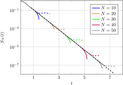
Figure 1: Universal relaxation function of the spin-helix amplitude (26) for different system sizes, in usual scale (top panel) and in logarithmic scale (bottom panel). Top Panel: Green, red and black dots correspond to $S_{6}(t),S_{8}(t),S_{10}(t)$ respectively, while the continuous curve shows $S(t)$ (33). The blue line is to be compared with Fig. 2a in [2]. Bottom Panel: $S_{N}(t)$ for $N=10,20,\ldots,50$, from (32), shows the exponential decay for large times, given by the black dashed line, (42). Coloured dashed curves show $S(r,t)$ with $r=[N/4]$ from (38). Curves with the same colour code correspond to the same $N$. Deviations from the straight line at large $t$ are due to finite size effects.

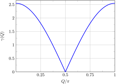
Figure 2: Asympotic decay rate $\gamma$ of the spin-helix state versus rescaled wavevector $Q/\pi$, given by $\frac{8}{\pi}|\cos(\pi x)|$. This Figure is to be compared with the Fig. 3c of [2].

Inserting $I=\sum_{\mathbf{p},M}\ket{\mu_{M}(\mathbf{p})}\bra{\mu_{M}(\mathbf{p})}$ in (26) and using (29) we obtain

$$S_{N}(t)=\sum_{\mathbf{p},\mathbf{q},M}\operatorname{e}^{{\rm i}(E_{\mathbf{p}}-E_{\mathbf{q}})t}\\ \times\left\langle\Omega|\mu_{M}(\mathbf{p})\right\rangle\bra{\mu_{M}(\mathbf{p})}\sigma_{1}^{x}\ket{\mu_{M}(\mathbf{q})}\left\langle\mu_{M}(\mathbf{q})|\Omega\right\rangle.$$ (30)

Next, we find that $\left\langle\Omega|\mu_{M}(\mathbf{p})\right\rangle=0$ unless $M=N/2$. After a lengthy calculation (see [10]) we eventually obtain

$$S_{N}(t)={\rm Re}[\det_{m,n=1,\dots,N/2}\phi^{(N)}_{m,n}(t)],$$ (31)

$$\phi^{(N)}_{m,n}=\frac{1}{N^{2}}\sum_{\begin{subarray}{c}p\in B_{+}\\ q\in B_{-}\end{subarray}}\frac{(1+\operatorname{e}^{-{\rm i}p})(1+\operatorname{e}^{{\rm i}q})\operatorname{e}^{{\rm i}[2(mp-nq)+t(\varepsilon_{p}-\varepsilon_{q}))]}}{\operatorname{e}^{{\rm i}(p-q)}-1},$$ (32)

where $\varepsilon_{p}=4\cos p$ and $B_{\pm}$ are sets of $p\in[-\pi,\pi)$ satisfying $\operatorname{e}^{{\rm i}pN}=\pm 1$. Eq. (32) describes the relaxation of the helix amplitude for finite periodic systems. Explicit expressions of $S_{N}(t)$ for $N=4,6$ are given in [10].

Interestingly, analyzing the Taylor expansion of $S_{N}(t)=\sum_{n}C_{N}(n)t^{n}$ at $t=0$ we observe that the Taylor coefficients for different $N$ follow the same stable pattern growing linearly with $N$. Namely, we find $C_{N+2}(n)=C_{N}(n)$ for $n=0,1,\ldots,2N-4$. Consequently, the stable pattern gives the exact Taylor expansion about $t=0$ of the decay of spin-helix amplitude in the thermodynamic limit

$$S(t)=\lim_{N\rightarrow\infty}S_{N}(t),$$ (33)

$$S(t)=\,1-4t^{2}+\frac{2^{5}}{3}t^{4}-\frac{2^{6}}{3}t^{6}+\frac{2^{9}}{15}t^{8}-\frac{2^{11}}{45}t^{10}+\frac{\ 2^{12}\,179}{14175}t^{12}$$

$$-\frac{2^{16}\,11}{14175}t^{14}+\frac{2^{16}2987}{4465125}t^{16}-\frac{2^{18}572}{4465125}t^{18}+\ldots,$$ (34)

obtainable also by direct operatorial methods.

Reduction to Bessel functions– For large $N$ the sums in (32) can be replaced by integrals. Then, after some algebra, we find that the entries $\phi^{(N)}_{m,n}(t)\rightarrow\phi_{m,n}(t)$ converge to (see [10])

$$(-1)^{m-n}\phi_{m,n}(t)=\delta_{m,n}+K_{m,n}(t),$$ (35)

$$K_{m,n}(t)=\frac{t}{m-n}\bigl{(}J_{2m}(4t)J_{2n-1}(4t)-J_{2n}(4t)J_{2m-1}(4t)\bigr{)}$$

$$+\frac{t}{m-n}\bigl{(}J_{2m-1}(4t)J_{2n-2}(4t)-J_{2n-1}(4t)J_{2m-2}(4t)\bigr{)}$$

$$+\frac{{\rm i}t}{m-n-1/2}\bigl{(}J_{2m-2}(4t)J_{2n}(4t)-J_{2n-1}(4t)J_{2m-1}(4t)\bigr{)}$$

$$-\frac{{\rm i}t}{m-n+1/2}\bigl{(}J_{2m-1}(4t)J_{2n-1}(4t)-J_{2n-2}(4t)J_{2m}(4t)\bigr{)},$$

$$K_{n,n}(t)=-(J_{0}(4t))^{2}+(J_{2n-1}(4t))^{2}+2\sum_{j=0}^{2n-2}(J_{j}(4t))^{2},$$ (36)

where the $J_{k}(x)$ are Bessel functions. After further manipulations (see [10]) and taking into account the symmetries of $K_{n,m}$ we finally obtain

$$S(t) =\lim_{r\rightarrow\infty}S(r,t)$$ (37)

$$S(r,t) =|\det_{m,n=1,\dots,r}A_{m,n}(t)|^{2},\,\,$$ (38)

$$A_{m,n}(t) =\delta_{m,n}+K_{m,n}(t)+K_{m,1-n}(t).$$ (39)

These formulae represent $S(t)$ as a product of two infinite determinants. Infinite determinants may define functions in very much the same way as infinite series. As in the present case, they may be extremely efficient in computations [14]. With a few lines of Mathematica code we obtain, e.g., $S(t=50)=7.64483\times 10^{-56}$ within a few seconds on a laptop computer. As opposed to the Taylor series (34) the determinant representation determines $S(t)$ for all times. The function $S(t)$ shown in Fig. 1 is directly comparable with the experimental data Fig. 2a in [2].

Even though the true thermodynamic limit is given by the limit $r\rightarrow\infty$ in (37), already for $r=1$ when the matrix $A$ is a scalar, the function

$$S(1,t) =g_{0}^{2}+4t^{2}\left(g_{0}+\frac{g_{1}}{3}\right)^{2},\quad g_{n}=J_{n}^{2}(4t)+J_{n+1}^{2}(4t)$$ (40)

approximates $S(t)$ for $0\leq t\leq 0.5$ (data not shown), and also reproduces the asymptotic Taylor expansion (34) up to the order $t^{7}$.

Choosing $r=4$ in (38) reproduces $S(t)$ with accuracy $|S(4,t)-S(t)|<10^{-5}$, for $t<2$ which is enough for any practical purpose. Indeed at $t=t_{max}=2$, the amplitude $S(t)$ drops by two orders of magnitude with respect to the initial value, $S(t_{max})\approx 0.0093<S(0)/100$. For larger $t$, $S(t)$ is well approximated by the asymptotics (42).

In addition, our numerics suggests a simple asymptotics for $\det A(t)$, namely

$$\det A(t)\rightarrow a_{0}\operatorname{e}^{2{\rm i}t}\operatorname{e}^{-\frac{4}{\pi}t},\quad t\gg 1,$$ (41)

$$a_{0}=1.2295\pm 2\times 10^{-5}.$$

The data were obtained by analyzing $\det A(t)$ for $r\leq 170$, and for times $t<t_{m}(r)=r/2.2-0.19$, data shown in [10]. Eq.(41) corresponds to the $S(t)$ asymptotics

$$\lim_{t\rightarrow\infty}S(t)\approx 1.5117\operatorname{e}^{-\frac{8}{\pi}t}.$$ (42)

From the asymptotics (42) and the self-similarity (23) we readily get the spin-helix state decay rate

$$\gamma(Q)=-\lim\limits_{t\rightarrow\infty}(t^{-1}{\log\langle\sigma_{n}^{x}(t)\rangle_{Q}})=\frac{8}{\pi}|\cos(Q)|,$$ (43)

shown in Fig. 2 and directly comparable with the experimental result, Fig. 3c of [2].

Conclusions– In this work, we propose a chiral qubit basis that possesses topological properties while retaining a simple factorized structure and orthonormality. The chiral basis at every site is represented by a pair of mutually orthogonal qubit states, and can be implemented with usual binary code registers. We demonstrate the effectiveness of the chiral basis by applying it to an experimentally relevant physical problem. Our results in Figs. 1 and 2 are compared to the experimental data.

As a byproduct of our study, we discovered the existence of a universal function $S(t)$ that governs the relaxation of transversal spin helices with arbitrary wavelengths in an infinite system under XX dynamics. We gave the explicit determinantal form of $S(t)$ (38) and calculated its Taylor expansion (34) and its large $t$ asymptotics (42). The possibility to express correlation functions in determinantal form is typical of integrable systems, see e.g. [15, 11, 16, 17, 18, 19]. We also obtained explicit expressions for the spin-helix state relaxation of finite systems of qubits (31) that can be useful for future experiments, such as those with ring-shaped atom arrays [20], where periodic boundary conditions can be realized.

Finally, in addition to applications to not yet solved problems it would also be interesting to check the performance of our chiral qubit basis towards problems already treated within traditional approaches e.g. [21, 22, 23].

References

Mallat [2009]S. Mallat, A Wavelet Tour of Signal
Processing: the Sparse Way, 3rd Revised edition (Academic Press, London, 2009).
Jepsen et al. [2022]P. N. Jepsen, Y. K. Lee,
H. Lin, I. Dimitrova, Y. Margalit, W. W. Ho, and W. Ketterle, Nature Physics 18, 899 (2022).
Jepsen et al. [2020]P. N. Jepsen, J. Amato-Grill,
I. Dimitrova, W. W. Ho, E. Demler, and W. Ketterle, NATURE 588, 403+ (2020).
Jepsen et al. [2021]P. N. Jepsen, W. W. Ho,
J. Amato-Grill, I. Dimitrova, E. Demler, and W. Ketterle, Phys. Rev. X 11, 041054 (2021).
Scholl et al. [2022]P. Scholl, H. J. Williams, G. Bornet,
F. Wallner, D. Barredo, L. Henriet, A. Signoles, C. Hainaut, T. Franz, S. Geier, et al., PRX Quantum 3, 020303 (2022).