Revealing contributions to conduction from transport within ordered and disordered regions in highly doped conjugated polymers through analysis of temperature-dependent Hall measurements

Abstract

Hall effect measurements in doped polymer semiconductors are widely reported, but are difficult to interpret due to screening of Hall voltages by carriers undergoing incoherent transport. Here, we propose a refined analysis for such Hall measurements, based on measuring the Hall coefficient as a function of temperature, and modelling carriers as existing in a regime of variable “deflectability” (i.e. how strongly they “feel” the magnetic part of the Lorentz force). By linearly interpolating each carrier between the extremes of no deflection and full deflection, we demonstrate that it is possible to extract the (time-averaged) concentration of deflectable charge carriers, $\left<n_{d}\right>$, the average, temperature-dependent mobility of those carriers, $\left<\mu_{d}\right>(T)$, as well as the ratio of conductivity that comes from such deflectable transport, $d(T)$. Our method was enabled by the construction of an improved AC Hall measurement system, as well as an improved data extraction method. We measured Hall bar devices of ion-exchange doped films of PBTTT-C₁₄ from 10 – 300 K. Our analysis provides evidence for the proportion of conductivity arising from deflectable transport, $d(T)$, increasing with doping level, ranging between 15.4% and 16.4% at room temperature. When compared to total charge-carrier-density estimates from independent methods, the values of $\left<n_{d}\right>$ extracted suggest that carriers spend $\sim$ 37% of their time of flight being deflectable in the most highly doped of the devices measured here. The extracted values of $d(T)$ being less than half this value thus suggest that the limiting factor for conductivity in such highly doped devices is carrier mobility, rather than concentration.

I Introduction

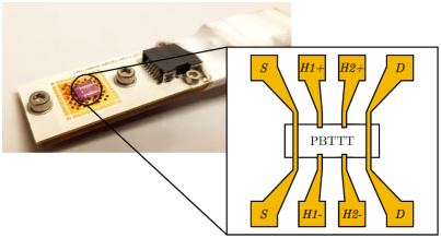
(a)

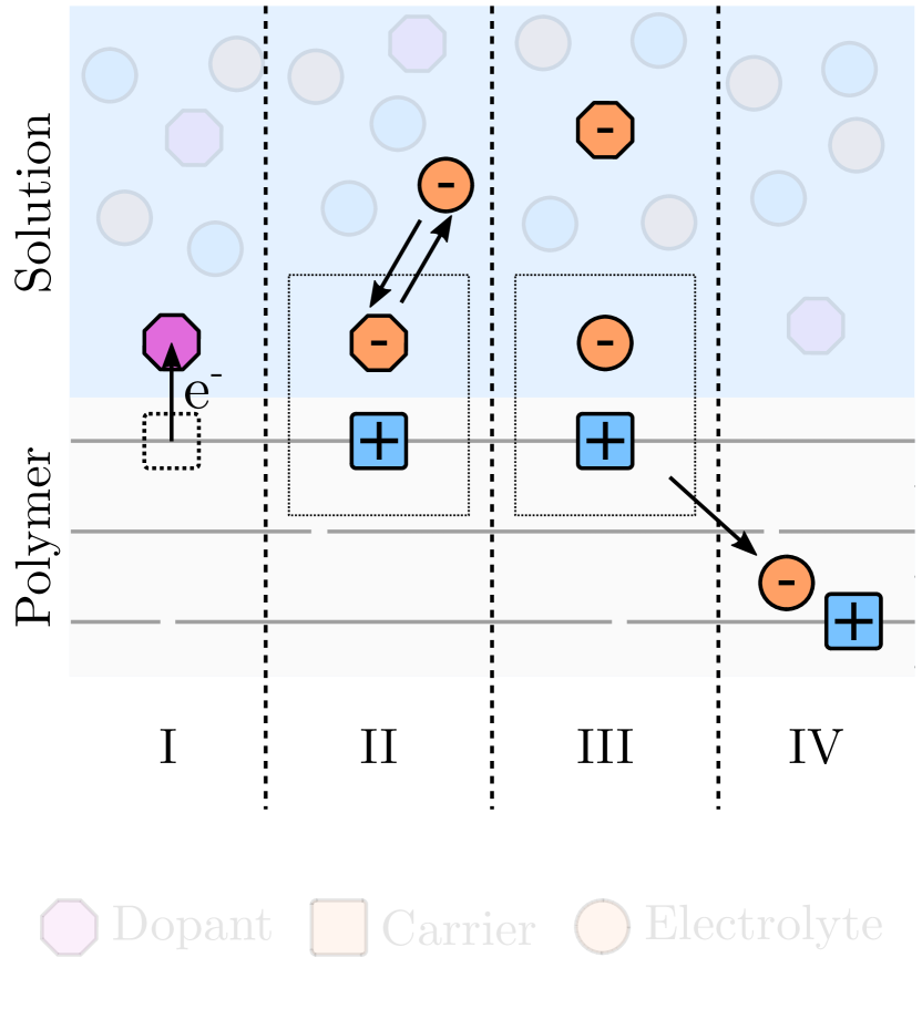
(b)

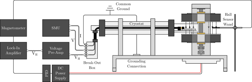
(c)

Figure 1: PBTTT Hall measurements: (1(a)) PBTTT Hall bar loaded on cryostat via custom-made sample board with device schematic displayed; (1(b)) Diagram displaying the stages of the ion-exchange doping process (I: charge transfer, II to III: exchange of ions, IV: charge carrier and exchanged ion diffuse into polymer); (1(c)) Diagrammatic representation of the AC Hall measurement system used for measurements.

Since the original, Nobel-prize-winning discovery of substantial electrical conductivities in polyacetylene by Heeger et al,[1] there has been continued interest in understanding the charge-transport physics of such degenerately doped, conjugated polymers. Recent advances in doping methods have focused on minimising structural disorder associated with incorporating dopant ions into polymer films, thus reaching optimal electrical conductivities. An example of this is the recently explored technique of ion-exchange (IEx) doping, where a polymer film is exposed to a solution containing both a molecular dopant and an electrolyte. After electron transfer from the polymer, the ionised molecular dopant is exchanged for a stable, closed-shell ion, which becomes the stabilising counterion for the mobile charge carriers on the polymer chains.[2, 3] This is depicted in Figure 1(b). IEx doping also provides a powerful method of systematically studying the influence of ion size and shape on polymer charge transport. This has enabled the identification of key factors that determine and limit achievable electrical conductivities.[4]

Hall effect measurements are normally a mainstay of semiconductor characterisation, with such measurements being used to determine charge-carrier densities and mobilities.[5, 6, 7] However, for conjugated polymers, these measurements are not straightforward to interpret, due to contibutions from disordered transport.[8, 9, 10] Attempting to use the standard single-carrier formulation, where the Hall coefficient is given by $R_{H}=[qn]^{-1}$, often leads to unreliable and unphysical estimates of carrier concentration. For instance, in their 2019 paper on IEx doping, Yamashita et al reported charge-carrier densities of $1.4\,\times\,10^{21}$ cm^-3 in their devices. However, XPS and NMR measurements published by Jacobs et al in 2022 have shown that in similarly doped devices of the same material, charge-carrier densities are actually closer to $8\times 10^{20}$ cm^-3 — about half that reported by the Hall measurements.[4] Similarly, carrier mobility extracted this way — often referred to as the “Hall mobility” — is consequently an underestimate. The strong temperature dependence of the Hall coefficient, and thus the measured carrier density, is inconsistent with spectroscopic measurements, underscoring the unreliability of these values.

It was shown by Yi et al in 2016[10] that the origin of such discrepancies, at least in molecular crystals, can be explained by the presence of charge carriers in localised electronic states. They suggested that localised carriers (in contrast to carriers in extended band-like states) do not partake in generating the transverse Hall voltage, but are still driven by its corresponding electric field. Therefore, they partially screen the Hall voltage leading to an underdeveloped Hall effect. Mathematically, they expressed this in terms of two parameters: $\gamma$ and $\beta$, the fraction of band-like carriers and ratio of localised to band-like mobility, respectively. The subsequent reduction in the measured Hall coefficient leads to an overestimation of carrier concentration and underestimation of carrier mobility. By taking certain temperature limits, Yi et al were able to formulate approximate expressions for their crystalline materials, allowing them to reliably extract carrier density and mobility values from their measurements.

A reliable means of estimating carrier density and carrier mobility is important for better understanding of the underpinning, fundamental charge-transport physics. Therefore, in an effort to achieve the same for IEx-doped polymer devices, we propose here to perform a similar analysis, thus requiring high-resolution, temperature-dependent measurements to be undertaken. This necessitated the construction of a new experimental system, based on the design first published by Chen et al in 2016[11] with some incremental improvements. These improvements were both to the hardware of the system, but also to the method of data processing used on its output, and are detailed later on.

For the analysis itself, we first show that an expression equivalent to that obtained from the $\beta$-$\gamma$ analysis of the two-carrier model can also be derived within a framework that is more appropriate for polymers — albeit with subtly different definitions of $\beta$ and $\gamma$. By making some reasonable assumptions about the arguments of the expression ($\beta$ and $\gamma$) we arrive at an approximate expression for the overall temperature dependence of the Hall coefficient. The analysis allows us to extract reliable values of charge-carrier density. We applied this method to highly conducting, IEx-doped films of poly(2,5)-bis(3-alkylthiophen-2-yl)thieno[3,2-b]-thiophene (PBTTT). We chose PBTTT due to it being a widely studied conducting conjugated polymer model system and our ability to determine carrier concentrations in IEx-doped PBTTT independently by spectroscopic means.

II Experimental System and Data Processing

There are a number of experimental challenges to performing temperature-dependent Hall measurements on conjugated polymers. Polymers are (relatively) electrically resistive materials, thus limiting the current densities that can be injected. This results in small Hall signals and subsequently low signal-to-noise ratios.[12, 13] This is normally mitigated by using superconducting electromagnets (SCEMs) to compensate for the low current densities. However, this is often not enough to fully compensate for the loss of signal. Therefore, the magnetic field would normally be ramped up and down slowly to the maximum accessible magnetic field, allowing for sufficiently large Hall voltage values to be measured as a function of time, and thus field. Such measurements normally take a prohibitively large amount of time to complete and are susceptible to electromagnetic interference and slow drift of signal. Additionally, slightly misaligned Hall electrodes on a device can cause issues if the longitudinal voltage is at all field-dependent. Specifically, magnetoresistance can often cause a greater change in longitudinal voltage with respect to field strength than in the Hall voltage itself — particularly at low temperatures.

A solution to both of these issues is offered by AC field measurements, in which the magnetic field is modulated (sinusoidally) on a time scale of $\sim 1$ s. The resulting modulation of the Hall voltage can then be detected with lock-in techniques. This spreads noise across the entire frequency domain while concentrating the Hall signal at a single frequency, thus significantly increasing the signal-to-noise ratio. Furthermore, since magnetoresistance is at least a second-order effect (i.e. $\sim O(B^{2})$), no contribution from it would be present at the field frequency.[14, 11] In Reference [11], Chen et al implemented this with an experimental design that used a rotating assembly of permanent magnets. These were aligned across two plates in an alternating fashion to generate an alternating magnetic field as it rotated. The RMS amplitude of the subsequently alternating Hall voltage was then measured by use of a lock-in amplifier, with reference signal provided by the analogue voltage output of a magnetometer.

In this work we made some iterative improvements upon this design (depicted in Figure 1(c)) to allow for temperature control and to further reduce noise. This improved system allowed us to take temperature-dependent Hall measurements at relatively high speeds ($\sim$ 1 day for a full temperature sweep), without magnetoresistance posing any issues, and with a greater signal-to-noise ratio. Specifically, the following additions were made:

1. A vacuum cryostat for temperature control and to prevent degradation of air-unstable devices;

2. Minimisation of enclosed area due to loop created by Hall voltage leads, including by use of twisted-pair, cryogenic-loom wiring;

3. An increased number of magnets per plate (4 instead of 2), resulting in a more accurately sinusoidal field and preventing the desired signal from being split across multiple harmonics;

4. A bespoke sample-loading mechanism, allowing for devices to be swapped in and out with relative ease (shown in Figure 1(a));

5. A high-impedance ($>1$ T$\Omega$) voltage pre-amplifier, allowing for measurement of low conductivity devices (down to $<1$ S/cm);

6. Software-based digital PID control to stabilise the rotational frequency of the magnet assembly, and hence field frequency.

Furthermore, improvements were made to the data-processing method used to extract the Hall coefficient from raw data. This could better separate out the Hall voltage from any Faraday-induced voltages and also allow for the sign of the Hall coefficient to be reliably determined.

To understand this, we must consider the main voltages that contribute to the measured output of such an AC Hall system: the Hall voltage itself, $V_{H}$, and voltages induced by the Faraday effect, $V_{F}$, due to changing magnetic fluxes.[11] Both oscillate at the same frequency as the field.[15, 16] To distinguish between the two contributions, it is important to note that only $V_{H}$ should depend on the source-drain current, $I$, and that $V_{F}$ will be $\pi/2$ out of phase with respect to $V_{H}$.[11] Since a dual-phase lock-in amplifier was used, both the in-phase ($V_{x}$) and $\pi/2$ out-of-phase ($V_{y}$) components of the signal are measured separately. One might then think that it is possible to directly measure $V_{H}$ separately from $V_{F}$ using this feature. However, since the reference signal used by the lock-in amplifier will have an arbitrary phase offset, $\phi$, from the field experienced by the device under test (DUT), this becomes non-trivial, with the vector voltage output becoming:

$$\mathbf{V}=\begin{bmatrix}V_{x}\\ V_{y}\end{bmatrix} =\begin{bmatrix}\cos{\phi}&-\sin{\phi}\\ \sin{\phi}&\cos{\phi}\end{bmatrix}\begin{bmatrix}V_{H}\\ V_{F}\end{bmatrix}$$ (1)

$$=\begin{bmatrix}V_{H}\cos{\phi}-V_{F}\sin{\phi}\\ V_{H}\sin{\phi}+V_{F}\cos{\phi}\end{bmatrix}.$$

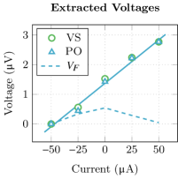
(a)

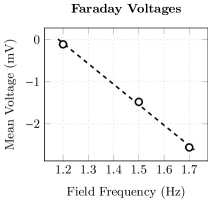
(b)

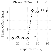
(c)

Figure 2: Data extraction from a Hall measurement: (2(a)) A seemingly trustworthy-looking measurement where both the vector-subtracted (VS) and phase-optimised (PO) data match closely and fluctuations in the Faraday voltage ($V_{F}$) are small relative to the Hall signal; (2(b)) Sign determination of a measurement, showing a negative gradient of Faraday voltage versus frequency indicating a positive Hall coefficient; (2(c)) A simulated example of what a change in $\textnormal{sgn}(R_{H})$ between two temperatures would look like in the calculated phase offset versus temperature — i.e. a jump in phase by a value of $\pi$ between the two temperatures.

To extract $V_{H}$ on its own will require an assumption to be made. The assumption made in Reference [11] was that $V_{F}$ is perfectly stable for a single measurement. The result of this is that by taking the vector differences of voltage measurements like so

$$|\Delta\mathbf{V}| =|\mathbf{V}(I_{1})-\mathbf{V}(I_{0})|$$ (2)

$$=\left|\begin{bmatrix}(V_{H}(I_{1})-V_{H}(I_{0}))\cos{\phi}\\ (V_{H}(I_{1})-V_{H}(I_{0}))\sin{\phi}\end{bmatrix}\right|$$

$$=|\mathbf{V}_{H}(I_{1})-\mathbf{V}_{H}(I_{0})|$$

$$=|\Delta\mathbf{V}_{H}|$$

one can find the magnitude of the Hall coefficient by finding the gradient of this vector difference versus current. Which value is used as the “zero” value is an arbitrary choice. For instance, one could simply take the first measurement in a sweep as being $\mathbf{V}(I_{0})$ and subtract it from all measured points.

This method is quick and can be performed live as data is acquired. However, the downside is that any noise in $V_{F}$ ends up being incorporated into the extracted $V_{H}$ signal. The assumption that $V_{F}$ is constant is also not entirely physical, as the moving parts in the system are liable to cause $V_{F}$ to fluctuate throughout a measurement via mechanical vibrations.

Alternatively, one could assume that the phase offset between the reference signal and DUT-experienced magnetic field is constant. If the position of the magnetometer sensor is fixed, then this would seem to be a more physical assumption. Further to this, if one assumes that $V_{F}$ fluctuates around a constant value, then it is possible to use numerical methods in an attempt to determine the phase offset, and separate $\mathbf{V}$ back into $V_{H}$ and $V_{F}$.

This can be formulated as a minimisation problem by defining a minimisation parameter, $P(\phi)$, to be

$$P(\phi)=\left|\dfrac{M_{y}(\phi)}{M_{x}(\phi)}\right|$$ (3)

where $M_{n}(\phi)$ is the gradient resulting from a linear fit of $V_{n}$ vs $I$ after rotating $\mathbf{V}$ through a phase $\phi$. The value of $\phi$ that minimises $P(\phi)$ should be the phase needed to rotate $\mathbf{V}$ through to separate out the Hall and Faraday components, since one would expect that $\left<\partial V_{F}/\partial I\right>\approx 0$ and $|\left<\partial V_{H}/\partial I\right>|\gg|\left<\partial V_{F}/\partial I\right>|$, where $\left<...\right>$ indicates a mean value.

Both methods have drawbacks. Vector subtraction (VS) is inherently noisier while phase optimisation (PO) may home in on the wrong value of $\phi$ if $V_{F}$ happens to have some sort of correlation with current (either by random chance or otherwise). Therefore, for each measurement performed using this system, both methods were used and their outputs compared. This provided a means of testing the reliability of a measurement. If the two outputs differed significantly or the extracted $V_{F}$ signal had large fluctuations relative to the $V_{H}$ signal, then the measurement was deemed unreliable. An example of a typical “trustworthy” measurement is shown in Figure 2(a).

In both methods explored thus far, it is only possible to tell the magnitude of the Hall coefficient — not its polarity. For VS, this is because only the magnitude of a vector is being found. For PO, this is because there is no way to tell whether $\phi$ or $\phi+\pi$ is the “correct” offset without more information. However, it should be possible to extract the sign of the Hall coefficient by checking how $V_{y}$ (Faraday) varies with frequency relative to how $V_{x}$ (Hall) varies with current. When properly aligned, the $x$ and $y$ components should be

$$V_{x} =R_{H}B_{z}I\sin(\omega t)/d$$ (4)

$$V_{y} =-\omega\Omega B_{z}\sin(\omega t+\pi/2)$$

where $R_{H}$ is the Hall coefficient, $\Omega$ is the cross-sectional area enclosed by the loop created by the Hall measurement wires, $B_{z}$ is the perpendicular magnetic flux density amplitude, $I$ is current, $\omega$ is the angular frequency of the field, $t$ is time and $d$ is the thickness of the DUT. If $R_{H}$ is positive, then the gradient of $V_{x}$ vs $I$ should have the opposite sign to the gradient of $V_{y}$ vs $\omega$. If it is negative then they will have the same sign. Therefore, after rotating through the determined value of $\phi$, the sign of $R_{H}$ can be determined from:

$$\textrm{sgn}(R_{H})=-\textrm{sgn}\left(\dfrac{\partial V_{y}}{\partial\omega}\dfrac{\partial V_{x}}{\partial I}\right).$$ (5)

Therefore, by performing frequency-dependent measurements one can extract the sign of the Hall coefficient as well as its magnitude.

This method was simplified for these measurements by always taking the value of $\phi$ that yields a positive Hall coefficient, then determining the sign by use of $\textrm{sgn}(R_{H})=-\textrm{sgn}(\partial V_{y}/\partial\omega)$. An example of this is shown in Figure 2(b). Further to this, only one frequency sweep at one temperature would be necessary, as any changes in sign of the Hall coefficient should result in whether $\phi$ or $\phi+\pi$ is the positive result changing. This would result in a “jump” in the selected phase offset by a value of $\pi$ between measurements. An illustration of what this would look like is shown in Figure 2(c). Therefore, if the sign is known at one temperature, the sign at all other temperatures can be determined by spotting these $\pi$-sized discontinuities in the phase offset versus temperature.

Given recent observations of n-type behaviour in some p-doped polymer Hall measurements[17], having the ability to determine the sign of $R_{H}$ was considered to be important for these measurements. This method was used on the PBTTT devices measured here to determine that the Hall coefficient was positive at all temperatures — as was expected.

While the devices measured in this work did not exhibit any noticeable frequency dependence in their Hall coefficients, it is conceivable that other devices may. In such cases, since frequency-dependent measurements will be necessary anyway, it is worth noting that extrapolating to zero frequency should effectively remove any influence of Faraday induction on the measured Hall signal (since $V_{F}\propto\omega$).

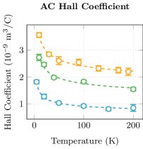
(a)

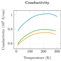
(b)

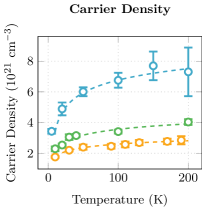
(c)

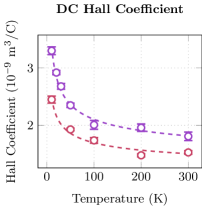
(d)

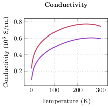
(e)

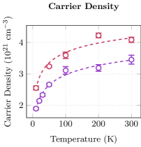
(f)

Figure 3: Plots of temperature-dependent data acquired from 5 IEx-doped Hall bar devices, 3 measured using the AC Hall system and 2 confirmatory measurements performed using a DC Hall system: (3(a) + 3(d)) Hall coefficient with fitted “guides for the eye” (dashed); (3(b) + 3(e)) Conductivity, (3(c) + 3(f)) Hall carrier density with fitted “guides for the eye” (dashed).

III PBTTT Hall Effect Measurements

Measurements were performed on devices of PBTTT-C₁₄, fabricated and doped using the methods described in Reference [3] using FeCl₃ as the molecular dopant and BMP TFSI as the electrolyte for IEx. The polymer films (thickness 40 nm) were patterned into a Hall bar shape (rectangle of length 900 $\muup$m, width 100 $\muup$m, with two pairs of bottom-contact Hall electrodes spaced equidistantly at 300 $\muup$m intervals along the channel, as shown in Figure 1(a)) using the methods described in Reference [18]. Three different films, doped to different levels of conductivity, were measured in the AC Hall system. Their room temperature conductivities (987 S/cm, 776 S/cm, and 719 S/cm) were high, with their temperature dependencies revealing metallic transport signatures. Specifically, at room temperatures, their conductivities decrease with increasing temperature and, at temperatures as low as 10 K, their conductivities retain values that are between $70-80\%$ of those at room temperature. As control measurements, two further devices were measured in a standard DC Hall system with a 12 T SCEM. The results of the AC Hall measurements are shown in Figures 3(a) to 3(c) and DC in Figures 3(d) to 3(f). The undoped thickness of the films was used to calculate $R_{H}$, as it should allow us to more readily compare results to other known quantities pertinent to the undoped film (such as monomer and polymer chain density).

For the AC measurements, temperature was swept from 10 K to 300 K in steps of 10 K. Previous tests had shown no hysteresis with temperature, thus it was only necessary to sweep in one direction. At each temperature step, the system would be left to stabilise for at least 30 minutes before performing any measurements. After stabilisation at each temperature, conductivity was measured, whereas Hall measurements were only performed (after conductivity) at a subset of steps (typically 10 K, 20 K, 30 K, 40 K, 50 K, 100 K, 150 K, and 200 K). This was because the low-temperature measurements were thought to be the most important for later analysis with values $>50$ K being less important.

The conductivity measurements were four-wire measurements performed using a Keithley 2450 source-measure unit (SMU), using its independent force and sense probes. For the Hall measurements, the voltage signal was extracted by use of a Stanford Research Systems SR830 lock-in amplifier via a SR551 voltage pre-amplifier ($>1$ T$\Omega$ input impedance) using a 30 s time constant (integration time) and $\pm 500$ $\muup$V sensitivity range, with current being injected by the previously mentioned SMU (now operating in two-wire mode).

The choice of frequency values to use was also important. Lower frequencies would require the use of longer integration times, as well as having to compete with greater $1/f$ noise. However, higher frequencies would result in greater noise from Faraday-induced voltages. It was found that a frequency of 1.2 Hz achieved a good balance between these competing factors, while still being reliably achievable using the DC motor (i.e. the motor and PID control were found to reliably and stably achieve this speed without stalling). Furthermore, minimising the area enclosed by the Hall voltage measurement loop — for instance by ensuring wire bonds were not overly long — helped minimise Faraday induction. For the room-temperature, frequency-dependent measurements, frequencies of 1.2 Hz, 1.5 Hz, and 1.7 Hz were used. Similarly, these values were chosen due to them being reliably achievable.

The data generally reveal good consistency between AC and DC measurements; both setups measure the same temperature dependence, thus showing the AC measurements in our new experimental setup to be reliable. The measurements show a pronounced negative correlation of $R_{H}$ with temperature, with this dependence becoming stronger at lower temperatures. This is consistent with what one should expect: as temperature decreases, the localised carriers (which move by a thermally-activated hopping transport mechanism) should become less mobile and thus less able to screen out the Hall voltage. The result of this screening is that at high temperatures the charge-carrier densities extracted by assuming the simple $R_{H}=[qn]^{-1}$ relation (plotted in Figures 3(c) and 3(f)) are clearly spurious. For instance, at 200 K the largest value of $\sim$ $8\times 10^{21}$ cm^-3 represents a density of $\sim$ $8$ carriers per monomer, since PBTTT typically has monomer densities $\sim$ $1\times 10^{21}$ cm^-3. That is, each monomer unit would need to be in a stable $+8$ oxidation state, which is chemically impossible.

IV Model Formulation

To develop a reliable method for analysing such Hall data, we first discuss the model for the under-developed Hall effect proposed in Reference [10]. This model, devised for crystalline organic small-molecule semiconductors, assumes the existence of two uniform populations of carriers: “band-like” carriers and localised, “hopping” carriers, denoted here with subscripts $b$ and $h$ respectively. By assuming that only band-like carriers experience a non-negligible contribution from the $\mathbf{v}\times\mathbf{B}$ term in the Lorentz force (for instance, one could argue that they have a negligibly small drift velocity), the Hall coefficient can be expressed as

$$R_{H}=\dfrac{n_{b}\mu_{b}^{2}}{q(n_{b}\mu_{b}+n_{h}\mu_{h})^{2}}$$ (6)

where $q$ is the charge on each carrier, $n_{b,h}$ are the respective charge-carrier densities, and $\mu_{b,h}$ are the respective charge-carrier mobilities. Then by defining the two parameters, $\beta$ and $\gamma$, with definitions

$$\beta=\dfrac{\mu_{h}}{\mu_{b}}\qquad\gamma=\dfrac{n_{b}}{n_{b}+n_{h}}$$ (7)

the Hall coefficient can be written as

$$R_{H}=\dfrac{1}{qn_{b}}\left[\dfrac{\gamma}{\gamma+(1-\gamma)\beta}\right]^{2}.$$ (8)

We now show that a very similar expression can be derived from a more generalised approach, which may be more suited to polymers. In this approach, instead of two uniform populations, we think of carriers as existing in a single population distributed on a continuous scale from completely localised to completely band-like. In an attempt to account for this, we assign each carrier a continuous and dimensionless “magnetic coupling parameter”, $g$, where $0\leq g\leq 1$, to quantify how strongly each carrier “feels” the magnetic term in the Lorentz force:

$$\mathbf{F}=q\left[\mathbf{E}+g\left(\mathbf{v}\times\mathbf{B}\right)\right].$$ (9)

By performing the usual derivation for the Hall effect (i.e. balancing transverse currents to zero)[19] and integrating over the total population of carriers, the Hall coefficient becomes

$$R_{H}=\dfrac{1}{qn_{t}}\dfrac{\int_{0}^{1}g\mu_{{}_{B}}^{2}(g)f(g)\,\textnormal{d}g}{\left[\int_{0}^{1}\mu_{{}_{E}}(g)f(g)\,\textnormal{d}g\right]^{2}}$$ (10)

where $n_{t}$ is the total charge-carrier density, and $f(g)$ is the distribution function describing the proportion of carriers that have a given value of $g$. It is worth noting that in this expression, we are implicitly assuming that carriers with different values of $g$ contribute to the conduction as channels in parallel. The subscripts of $\mu$ — $E$ and $B$ — are introduced to keep track of which mobility values pertain to acceleration from the electric and magnetic parts of the Lorentz force respectively. For instance, if one were to assume that electric fields are able to accelerate carriers for their entire time of flight, but only for a portion of it for magnetic fields, then a carriers average mobility as “seen” by magnetic fields will not necessarily be the same as “seen” by electric fields (as they will be averaged over different periods of time).

Regardless of assumption, it can be seen that the integrals in Equation 10 are over the entire domain of, and contain, the distribution function, $f(g)$. Therefore, they can be written as expectation values, allowing us to write

$$R_{H}=\dfrac{1}{qn_{t}}\dfrac{\left<g\mu^{2}_{{}_{B}}\right>}{\left<\mu_{{}_{E}}\right>^{2}}$$ (11)

thus showing that the “normal” Hall coefficient ($[qn_{t}]^{-1}$) is reduced by an interplay between the most-delocalised carriers providing the greatest contribution to the numerator, $\left<g\mu^{2}_{{}_{B}}\right>$, due to being weighted by $g$, and the least-delocalised carriers contributing significantly only to the denominator, $\left<\mu_{{}_{E}}\right>^{2}$.

Equations 10 and 11 should be thought of as general (albeit abstract) expressions for describing the under-developed Hall effect in single-carrier, partly disordered materials. The intricacies of how it applies to a specific material, then, are to be found in what functional form its important parameters (i.e. $\mu_{{}_{E,B}}(g)$ and $f(g)$) are assumed to take. For instance, if one were to assume that

$$n_{t}f(g) =n_{b}\delta(g-1)+n_{h}\delta(g)$$ (12)

$$\mu_{{}_{E}} =\mu_{{}_{B}}=\left\{\begin{matrix}\mu_{h}&\textnormal{for}\,g=0\\ \mu_{b}&\textnormal{for}\,g=1\end{matrix}\right.$$

where $\delta(x)$ is the Dirac delta distribution, then the expression will reduce back to that in Equation 8 with $\gamma=f(1)/(f(0)+f(1))$ and $\beta=\mu(0)/\mu(1)$. Therefore, the two-carrier model can be thought of as being the result of binning all carriers into having either $g=0$ or $g=1$ (i.e. being either fully localised or fully delocalised).

However, in polymers such as PBTTT, charge transport is often thought of as occuring along conductive pathways, or “fibrils”, comprising different sections where carriers undergo different modes of transport (typically band-like, hopping, and disordered-metallic).[20] Properties, such as resistivity, are then predicted by adding these contributions together in series, weighted by the fraction of the fibril they account for. Therefore, for the Hall coefficient, we took a similar approach by assuming that $g$ comes about due to a carrier only spending a proportion $g$ of its time of flight moving via mode(s) of transport under which the magnetic field is able to deflect it.

To model this, we define $\left<\mu_{d}\right>$ to be the average mobility of carriers when they are undergoing such “deflectable” transport, and $\left<\mu_{n}\right>$ to be that when they are undergoing “non-deflectable” transport. Therefore, by assuming that carriers are always being driven be electric fields, regardless of transport mechanism, we can write $\mu_{{}_{E}}$ as the weighted average of both average mobilities:

$$\mu_{{}_{E}}(g)=g\left<\mu_{d}\right>+(1-g)\left<\mu_{n}\right>.$$ (13)

Similarly, by assuming that magnetic fields effectively only act on the carrier when it is travelling via deflectable mechanisms, we equate $\mu_{{}_{B}}$ to the average deflectable mobility only:

$$\mu_{{}_{B}}(g)=\left<\mu_{d}\right>.$$ (14)

Then, by defining $\int_{0}^{1}gf(g)\textnormal{d}g=\left<g\right>$, and $b=\left<\mu_{n}\right>/\left<\mu_{d}\right>$, the Hall coefficient can now be expressed as

$$R_{H}=\dfrac{1}{q\left<n_{d}\right>}\left[\dfrac{\left<g\right>}{\left<g\right>+(1-\left<g\right>)b}\right]^{2}$$ (15)

where $\left<n_{d}\right>=\left<g\right>n_{t}$ is the average effective deflectable carrier density — that is the average density of carriers that are deflectable at any given moment in time. This expression is very similar to that derivable from Reference [10], with the only difference being that $\gamma$ and $\beta$ have been substituted with $\left<g\right>$ and $b$ respectively.

This implies that by allowing carriers to exist anywhere in a linear interpolation between the fully-localised and fully-delocalised states previously assumed, one still arrives at the same functional form — albeit with subtly different definitions to its arguments. That is, the value of $\left<g\right>$ or $\gamma$ may be thought of as an average measure of the overall delocalisation of carriers, as opposed to the fraction of carriers that are fully delocalised. Therefore, the two-carrier functional form from Reference [10] should be usable for polymers so long as these different definitions are kept in mind. To emphasise this, from this point onward, we shall use the notation $\left<g\right>$ and $b$ instead of $\gamma$ and $\beta$.

V Relating to Physical Quantities

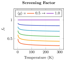
(a)

(b)

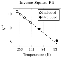
(c)

Figure 4: Various plots of the theoretical temperature dependence of the Hall screening factor with $D=0.25$, $T_{*}=1$ K, $b_{\infty}=1$, and $\left<g\right>=0.5$ unless stated otherwise: (4(a)) Plotted as a function of temperature for $0.5\leq\left<g\right>\leq 1.0$, (4(b)) Plotted logarithmically against $T^{-D}$ demonstrating a linear relationship for small $T^{-D}$ or large $T$, (4(c)) Plotted as its inverse square against $T^{-D}$ again showing a linear relationship for small $T^{-D}$ or large $T$.

With just two independent experimental measurements at each temperature ($R_{H}$ and $\sigma$) it is not possible to extract the three model parameters ($\left<n_{d}\right>$, $\left<g\right>$ and $b$) unambiguously. Therefore, it is necessary to make further assumptions. Since the polymer systems in question are highly doped – implying that the Fermi energy is large compared to $k_{B}T$ — it is unlikely that a change in temperature will affect the distribution of carriers across different modes of transport much. Therefore, we assume $\left<g\right>$ to be mainly a function of carrier concentration, and independent of temperature. On the other hand $b$, being a ratio of mobility values, is likely to be a strong function of temperature only:

$$\left<g\right>\approx\left<g\right>(n_{t})\qquad b\approx b(T).$$ (16)

Finding an appropriate functional form for $b(T)$ requires us to consider which scenarios, that a charge carrier might find itself in, would result in deflectable and non-deflectable transport. The simplest pair of contrasting scenarios would be when a carrier is undergoing localised, variable-range-hopping-like transport versus delocalised, band-like transport. In the former case, such carriers would not have a coherent enough wavevector to be deflected by a magnetic field, whereas in the latter case they would. Thus, it may be tempting to suggest that $\left<\mu_{n}\right>$ should arise from hopping-like transport and $\left<\mu_{d}\right>$ from band-like transport. However, there are other factors in polymers that may cause a carrier to become non-deflectable.

For instance, polarons in different regions of the polymer with differing amounts of structural disorder, will have differing degrees of delocalisation, while quite possibly still having band-like mobilities. Similarly, the effect of transient (de)localisation may be such that otherwise localised carriers, being excited into band-like states temporarily, do not remain in such delocalised states long enough to be fully deflected by magnetic fields. Whatever the case, it is clear that which mobility contributions should be categorised into the “deflectable” and “non-deflectable” categories is not as obvious as just deflectable being band-like and non-deflectable being hopping-like. Therefore, a better approach may be a semi-empirical one, where we choose a functional form of $b(T)$ based on the behaviour of the measured data.

Since the functional form, when incorporated into Equation 15, will take the form $\sim\left[1+b(T)\right]^{-2}$ we will want a function for $b(T)$ that is small with a strong temperature dependence at low temperatures, while plateauing at higher temperatures. A good fit for this would be an exponential function, similar to that used for variable-range hopping:

$$b(T)\approx b_{\infty}\exp{\left\{-\left[\dfrac{T_{*}}{T}\right]^{D}\right\}}$$ (17)

where $b_{\infty}$, $T_{*}$, and $D$ are all positive constants to be fitted. At low $T$ ($T\lesssim T_{*}$) this function has a small value ($b(T)\rightarrow 0$ as $T\rightarrow 0$) with a strong temperature dependence, and at high temperatures ($T\gg T_{*}$) it plateaus asymptotically towards $b_{\infty}$.

Taking this functional form for $b(T)$ yields an approximate expression for the Hall coefficient given by:

$$R_{H}(T)\approx R_{H}^{0}\left[\dfrac{\left<g\right>}{\left<g\right>+(1-\left<g\right>)b_{\infty}e^{-\left(T_{*}/T\right)^{D}}}\right]^{2}$$ (18)

where $R_{H}^{0}$ has been introduced as the “deflectable Hall coefficient” given by $R_{H}^{0}=[q\left<n_{d}\right>]^{-1}$. For convenience, we also define $f_{s}(T)=R_{H}(T)/R_{H}^{0}$ as the “screening factor”. To illustrate the expected dependence of the Hall coefficient on temperature, we choose an example with parameters $b_{\infty}=1$, $T_{*}=1$ K, $D=0.25$, and $0.5\leq\left<g\right>\leq 1.0$, allowing us to plot $f_{s}$ against temperature in Figure 4(a). Qualitatively, its behaviour is in good agreement with the measured data, providing assurance that it might be possible to fit the data to this model.

It should now be possible to attempt extracting the values of the functions parameters by fitting to temperature-dependent Hall coefficient data. However, it is still important to note that in this model, there are 5 parameters:

1.	$T_{*}$	The mobility-ratio temperature coefficient;
2.	$D$	The mobility-ratio temperature exponent;
3.	$b_{\infty}$	The mobility ratio value as $T\rightarrow\infty$;
4.	$\left<g\right>$	The mean magnetic coupling parameter;
5.	$R_{H}^{0}$	The deflectable Hall coefficient.

Therefore, to achieve a reliable fit it was important to constrain some of their values via alternative methods. This was done by approximating the full expression in certain temperature limits. For instance, when $b(T)\gg\left<g\right>/(1-\left<g\right>)$ (i.e. when non-deflectable transport is dominating), the expression can be approximated as

$$R_{H}\approx R_{H}^{0}\left[\dfrac{\left<g\right>}{b_{\infty}(1-\left<g\right>)}\right]^{2}\exp{\left\{2\left[\dfrac{T_{*}}{T}\right]^{D}\right\}}$$ (19)

which was used to fit the “guides for the eye” in Figures 3(a) and 3(d). Following this, $D$ can now be estimated by finding the value that gives the most linear fit of $\ln{(R_{H})}$ against $T^{-D}$, allowing $T_{*}$ to then be estimated by use of

$$T_{*}\approx\left[\dfrac{1}{2}\dfrac{\partial\ln{(R_{H})}}{\partial T^{-D}}\right]^{\frac{1}{D}}$$ (20)

which can be calculated using a linear fit, an example of which is shown in Figure 4(b).

Following from this, if one assumes to be in the limit of $T\gg T_{*}$, then $R_{H}^{0}$ can be estimated by fitting $R_{H}^{-1/2}$ against $T^{-D}$ to yield a linear relation of

$$R_{H}^{-1/2} \approx MT^{-D}+C$$ (21)

$$M =-\left(R_{H}^{0}\right)^{-\frac{1}{2}}\left(\left<g\right>^{-1}-1\right)b_{\infty}T_{*}^{D}$$

$$C =\left(R_{H}^{0}\right)^{-\frac{1}{2}}-\dfrac{M}{T_{*}^{D}}$$

thus allowing for $R_{H}^{0}$ to be estimated from

$$R_{H}^{0}\approx\left[C+\dfrac{M}{T_{*}^{D}}\right]^{-2}$$ (22)

an example fit of which is shown in Figure 4(c).

At this point, three out of five parameters have been estimated, thus reducing the fitting problem to a relatively simple two-variable one. However, $\left<g\right>$ and $b_{\infty}$ are not uniquely solvable. This can be seen by dividing Equation 18 through by $\left<g\right>^{2}$ to give:

$$R_{H}(T)\approx R_{H}^{0}\left[1+he^{-(T_{*}/T)^{D}}\right]^{-2}$$ (23)

where we have defined $h$ to be

$$h=\dfrac{1-\left<g\right>}{\left<g\right>}b_{\infty}.$$ (24)

Different value pairs of $\left<g\right>$ and $b_{\infty}$ can be chosen and, so long as they produce the same value of $h$, they will produce the same fit. Therefore, the true fitting parameter is $h$. By considering the meanings of the parameters that make up $h$, one can arrive at

$$he^{-(T_{*}/T)^{D}}=\dfrac{\sigma_{n}(T)}{\sigma_{d}(T)}$$ (25)

where $\sigma_{n,d}$ are the temperature-dependent contributions to conductivity from non-deflectable and deflectable transport respectively. We can then rearrange to give the fraction of conduction that is deflectable, as a function of temperature, the result of which can be seen to equal the square root of the screening factor, $f_{s}$:

$$d(T)=\dfrac{\sigma_{d}}{\sigma_{d}+\sigma_{n}}=\left[1+he^{-(T_{*}/T)^{D}}\right]^{-1}=\sqrt{f_{s}}.$$ (26)

Furthermore, Equation 25 allows us to calculate $\left<\mu_{d}\right>$ as a function of temperature by use of

$$\left<\mu_{d}\right>(T)=\dfrac{\sigma(T)R_{H}^{0}}{1+he^{-(T_{*}/T)^{D}}}$$ (27)

where $\sigma(T)$ is the measured temperature-dependent conductivity.

By considering temperature limits, it can be seen that Equations 25 taken in the limit of $T\gg T_{*}$ — that is when it has plateaued — simply gives $h$. Therefore, $h$ on its own can be a useful parameter, since Equation 26 can then be estimated by:

$$d(T\gg T_{*})\approx(1+h)^{-1}.$$ (28)

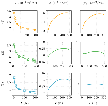
	$D$	$T_{*}$ (K)
1	$0.299\pm 0.019$	$1.34\pm 0.10$
2	$0.239\pm 0.018$	$1.35\pm 0.20$
3	$0.226\pm 0.030$	$1.31\pm 0.21$
	$R_{H}^{0}$ (m3/C)	$\left<n_{d}\right>$ (cm-3)
1	$(5.72\pm 0.29)\times 10^{-8}$	$(1.09\pm 0.05)\times 10^{20}$
2	$(5.08\pm 0.48)\times 10^{-8}$	$(1.23\pm 0.12)\times 10^{20}$
3	$(1.87\pm 0.10)\times 10^{-8}$	$(3.34\pm 0.18)\times 10^{20}$
	$1/[1+h]$ (%)	$\left<\mu_{d}\right>$ (cm2/Vs)
1	$15.4\pm 0.21$	$2.95-6.33$
2	$16.2\pm 0.37$	$7.43-7.94$
3	$16.4\pm 0.92$	$3.78-4.05$

Figure 5: The results of fitting the Hall data acquired from three IEx-doped PBTTT hall bars, with plots of Hall coefficient ($R_{H}$), conductivity ($\sigma$) and mean deflectable mobility ($\left<\mu_{d}\right>$) on the left, and a table of fitted parameters on the right.

If $T_{*}$ is much smaller than room temperature, then this value should accurately estimate the fraction of conductivity that is deflectable at room temperature.

Estimating $h$ can be done with the approximate expression in Equation 19 by realising that the prefactor to its exponential is equal to $R_{H}^{0}h^{-2}$. Therefore, we have managed to estimate all fitting parameters, making a fit of the full expression relatively simple. However, the limits in which these approximations apply cannot be determined until the values they approximate have been calculated. Therefore, the estimates they provided would often constitute visually poor fits.

To combat this, an iterative, self-consistent approach was employed. After computing the estimates described above, using all available data points, the resulting values were then used to calculate the limits. Data points would then be removed from the fits based on these new limits and the process repeated and the limits re-calculated. Data points would then be removed again (or at this point possibly re-added) based on the new limit values. This would repeat until no further changes occurred — that is the results became self-consistent. In some cases, where such a method would lead to all points being removed in early iterations (causing the process to terminate prematurely), a more simplistic approach of removing low-temperature points one by one would be used until the estimates became self-consistent.

After this, fits would normally still appear visually to be sub-optimal, thus a final, generalised fitting would be run. In this, the whole expression would be fit to, using a least-squares, Nelder-Mead optimisation function. The previously estimated values would be used as the initial values for the fit, with their values being constrained to remain within 30% of these values.

VI Results

By performing the self-consistent analysis presented in the previous section, three sets of Hall data from Figures 3(a) and 3(d) were fitted (with maximum conductivities: $\sim$ 600 S/cm, $\sim$ 750 S/cm, $\sim$ 1000 S/cm). The other two sets of data proved to have too few points and too much noise to reliably fit. The results of these fittings are shown in Figure 5.

Focusing first on the values of $T_{*}$, it should be possible to glean some insights. In our chosen function for $b(T)$, $T_{*}$ controls the temperature above which the ratio of non-deflectable to deflectable mobilities plateaus and becomes relatively temperature independent. Therefore, a greater value of $T_{*}$ would correspond to a system that requires a greater value of temperature to achieve relatively temperature-independent transport. Therefore, it could be said that a greater value of $T_{*}$ indicates a greater amount of energetic disorder, with its transport remaining thermally activated for greater values of temperature. Following this line of logic, all three devices have similar, small values of $T_{*}$, with a slight decrease being apparent at the greatest conductivity, albeit within the error ranges of the other two devices. The small values of $T_{*}$ here (relative to room temperature) indicate relatively low levels of disorder overall. If the decrease in device 3 can be trusted, it would suggest that the energetic disorder of such systems continues to decrease with increased doping. This is all consistent with our recent study of the charge-transport physics of IEx-doped conjugated polymers, including PBTTT,[3, 4] where grazing-incidence wide-angle x-ray scattering (GIWAXS) measurements of IEx-doped PBTTT films showed reduced $\pi-\pi$ stacking disorder at high doping concentrations. There is also evidence that the intrachain and interchain polaron delocalisation lengths become very long at high doping concentrations allowing the charges to average effectively over individual Coulomb wells and reducing the energetic disorder felt by the carriers. This would also appear to be supported by the value of $1/(1+h)$ increasing slightly with doping concentration, from 15.4% to 16.4%, which would indicate a greater degree of deflectable transport contributing to conduction. However, the errors on these values overlap, hence it is hard to say with any certainty if this is truly what is happening in these data, or whether this is simply due to random error.

The maximum $\left<\mu_{d}\right>$ values extracted here range around $\mu$ $\sim$ 4 – 8 cm${}^{2}/$Vs. This is consistent with mobilities estimated from carrier densities measured by XPS previously (6 – 8 cm${}^{2}/$Vs) and an order of magnitude greater than typical values for undoped PBTTT in FET architectures.[21] This similarly supports the idea that these doped films exhibit significantly less energetic disorder as a result of their doping. Furthermore, the two most highly doped devices here exhibit a significantly less temperature-dependent deflectable mobility than the least doped device. This similarly suggests that these devices exhibit a greater amount of order, with deflectable transport becoming more band-like in its temperature dependence at greater doping levels. This finding has important implications: it shows that a new regime has been reached, where not only does doping to high concentrations not disrupt the crystalline and energetic order of the polymer, but goes so far as to enhance it. In previous work on solid-state-diffusion-doped PBTTT,[22] where only the uncorrected values of Hall mobility were available for analysis (with those values being underestimates and effectively only acting as a lower bound on the true value) it was only possible to conclude that doping did not significantly disrupt the lattice structure of the polymer.[22] Now that more meaningful values of mobility can be extracted, as well as $T_{*}$ and $1/(1+h)$, it is clear that this may have been something of an understatement.

The values of $\left<n_{d}\right>$ for all three devices are much more physically reasonable values than those extracted by simply assuming $R_{H}=[qn]^{-1}$ in Figures 3(c) and 3(f). By assuming a monomer density of $\sim 1\times 10^{21}$ cm^-3, estimated from the polymer film density, these suggest that devices 1, 2 and 3 (on average) have roughly one deflectable polaron per 9, 8, and 3 monomer sites respectively.

Further to this, the total charge-carrier density of a PBTTT device, similarly doped to device 3 here, was measured in our previously mentioned, recent charge-transport study[4] using x-ray photoemission spectroscopy (XPS) and nuclear magnetic resonance (NMR). By determining the concentration of TFSI^- anions in the film, its total charge-carrier density was determined to be $n_{t}=(8.84\pm 0.24)\times 10^{20}$ cm^-3. Since $\left<n_{d}\right>=\left<g\right>n_{t}$, this would suggest that device 3 has a value of $\left<g\right>\approx 0.37$. That is, carriers spend $\sim$ 37% of their time moving deflectably. Following from this, the result here of deflectable transport only accounting for $\sim$ 16% of the conductivity despite carriers being in such states for $\sim$ 37% of the time, suggests that the carriers undergoing less deflectable transport may in fact exhibit higher carrier mobilities than those in more deflectable pathways. This is not necessarily a contradiction, as more deflectable pathways are likely to consist of more highly ordered, crystalline polymer domains that support more delocalised carriers, but may not be well interconnected. This also suggests that the limiting factor on conductivity in such deflectable pathways is mobility rather than charge-carrier density. This further solidifies the observation in our previous study that the limit of conductivity enhancement that can be achieved by adding charge carriers has been reached with IEx doping. Indeed, the fact that the most highly doped device here (device 3) has a significantly smaller maximum deflectable mobility than the other two, lesser-doped devices suggests that something of a trade-off is occurring between carrier density and mobility — where greater carrier densities provide diminishing returns on their enhancement of conductivity.

VII Conclusions

We have presented a new methodology for interpreting Hall effect measurements on highly doped PBTTT, based on analysing temperature-dependent Hall data. To provide said data, we have developed an improved AC Hall measurement system and data-extraction routine, allowing measurements of the Hall effect from 10K to room temperature with high signal-to-noise ratios. Using PBTTT as a model system we have shown that the improved Hall analysis is able to determine the “deflectable” carrier concentration and mobility. Not only that, but our method also provides insight into how “ideal” the transport of charge carriers is by allowing us to estimate the relative contributions to the total conductivity from more ordered regions of the polymer, where carriers can be deflected by magnetic fields, and from less ordered regions where they cannot. Our method and analysis promises to transform the Hall effect from a finicky and hard-to-interpret transport phenomenon in polymer semiconductors, into a valuable tool for understanding and optimising such materials in the future.