Continuity of Thresholded Mode-Switched ODEs and Digital Circuit Delay Models

Abstract.

Thresholded mode-switched ODEs are restricted dynamical systems that switch ODEs depending on digital input signals only, and produce a digital output signal by thresholding some internal signal. Such systems arise in recent digital circuit delay models, where the analog signals within a gate are governed by ODEs that change depending on the digital inputs.

We prove the continuity of the mapping from digital input signals to digital output signals for a large class of thresholded mode-switched ODEs. This continuity property is known to be instrumental for ensuring the faithfulness of the model w.r.t. propagating short pulses. We apply our result to several instances of such digital delay models, thereby proving them to be faithful.

1. Introduction

A natural class of hybrid systems can be described by the dynamics of a continuous process, which is controlled by externally supplied digital mode switch signals, and provides a digital output based on whether some internal signal crosses a threshold, see Fig. 1 for an illustration. Examples are digitally controlled thermodynamic processes, hydrodynamic systems, and, in particular, digital integrated circuits. The continuous dynamics of these systems are described by Ordinary Differential Equations (ODEs) for the temperature, the pipe’s pressures and fill-levels, or the gate’s currents and voltages over time. Digital mode switches are used to switch between ODE systems, e.g., by turning on a heater, closing a valve, or applying an input transition to a gate’s input. The environment of the hybrid system is only notified if the temperature or fill-level crosses a threshold, or, in the case of a digital gate, is said to produce an output transition when some internal voltage crosses a threshold.

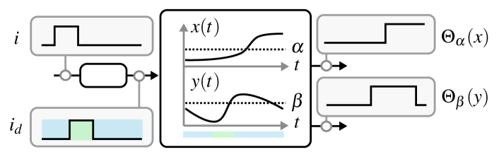
Figure 1. Thresholded mode-switched ODE with a single mode input $i$, the delayed input $i_{d}$, two continuous states $x,y$, and two thresholded outputs $\Theta_{\alpha}(x)$ and $\Theta_{\beta}(y)$.

In this work, we consider the composition of such hybrid systems in a circuit, where digital threshold signals of one component drive mode switch signals of a downstream component. We give conditions that ensure the continuity of the outputs of such circuits with respect to their inputs and provide two application examples in the context of circuit delay models. The proven continuity property shows that small variations of the inputs lead to small variations of the output signal, a property that is necessary for digital circuit models to be consistent with physical analog ODE models.

Digital circuits, continuity, and faithful delay models. Analog simulations of digital circuits are time-consuming and are thus replaced by digital simulations whenever possible. Typical application domains that require simulation of precise circuit transition times are particularly timing-critical, asynchronous parts of a circuit, e.g., inter-neuron links using time-based encoding in hardware-implemented spiking neural networks (BVMRRVB19), where the worst-case delay estimates provided by static timing analysis techniques are not sufficient for ensuring correct operation.

A mandatory prerequisite for dynamic timing analysis are digital delay models, which allow to accurately determine the input-to-output delay of every constituent gate in a circuit. Suitable models must also account for the fact that the delay of an individual signal transition usually depends on the previous transition(s), in particular, when they were close. The simplest class of such models are single-history delay models (FNS16:ToC; BJV06; FNNS19:TCAD), where the input-to-output delay $\delta(T)$ of a gate depends on the previous-output-to-input delay $T$.

It has been proved by Függer et al. (FNNS19:TCAD) that a certain continuity property of single-history models is mandatory for the digital abstraction to faithfully model the analog reality. In particular, the predicted output transitions must not be substantially affected by arbitrarily short input glitches. For example, the constant-low input signal and an arbitrarily short low-high-low pulse must produce arbitrary close gate output signals. So far, the only delay model known to ensure this continuity property is the involution delay model (IDM) (FNNS19:TCAD), which consists of zero-time Boolean gates interconnected by single-input single-output involution delay channels. An IDM channel is characterized by a delay function $\delta$, which is a negative involution, i.e., $-\delta(-\delta(T))=T$. In its generalized version, different delay functions $\delta_{\uparrow}$ resp. $\delta_{\downarrow}$ are assumed for rising resp. falling transitions, requiring $-\delta_{\uparrow}(-\delta_{\downarrow}(T))=T$. Unlike all other existing delay models, the IDM has been proved to faithfully model glitch propagation for the so-called short-pulse filtration problem (FNNS19:TCAD), and is hence the only candidate for a faithful delay model known so far (FNS16:ToC).

It has also been shown (FNNS19:TCAD) that involution delay functions arise naturally in a 2-state thresholded hybrid channel model, which consists of a pure delay component, a slew-rate limiter with a rising and falling switching waveform, and an ideal comparator (Fig. 2): The binary-valued input $i_{a}$ is delayed by $\delta_{\mathrm{min}}>0$, which assures causality of channels, i.e., $\delta_{\uparrow/\downarrow}(0)>0$. For every transition on $i_{d}$, the generalized slew-rate limiter switches to the corresponding waveform ($f_{\downarrow}/f_{\uparrow}$ for a falling/rising transition). The essential property here is that the analog output voltage $o_{a}$ is a continuous (but not necessarily smooth) function of time. Finally, the comparator generates the output $o_{d}$ by digitizing $o_{a}$ w.r.t. the discretization threshold voltage $V_{th}$.

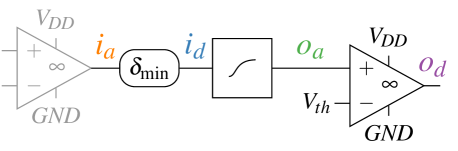
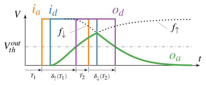
Figure 2. Hybrid involution delay channel model (upper part) with a sample execution (bottom part). Adapted from (FNNS19:TCAD).

Whereas the accuracy of IDM predictions for single-input, single-output circuits like inverter chains or clock trees turned out to be very good, this is less so for circuits involving multi-input gates (OMFS20:INTEGRATION). It has been revealed by Ferdowsi et al. (FMOS22:DATE) that this is primarily due to the IDM’s inherent lack of properly covering output delay variations caused by multiple input switching (MIS) in close temporal proximity (CGB01:DAC), also known as the Charlie effect: compared to the single input switching case, output transitions are sped up/slowed down with decreasing transition separation time on different inputs. Single-input, single-output delay channels like IDM cannot exhibit such a behavior.

To capture MIS effects in a 2-input NOR gate, Ferdowsi et al. (FMOS22:DATE) hence proposed an alternative digital delay model based on a 4-state hybrid gate model. It has been obtained by replacing the 4 transistors in the RC-model of a CMOS NOR gate by ideal zero-time switches, which results in one mode per possible digital state of the inputs $(A,B)\in\{(0,0),(0,1),(1,0),(1,1)\}$. In each mode, the voltage of the the output signal and an internal node are governed by constant-coefficient first order ODEs. When an input signal changes its state, the system switches to the new mode and its corresponding ODEs.

Albeit digitizing this hybrid gate model, using a comparator with a suitable threshold voltage $V_{th}$ as in Fig. 2, leads to a quite accurate digital delay model, it turned out to still fail to capture the MIS delay for a rising output transition. In a follow-up paper (ferdowsi2022accurate), Ferdowsi et. al. hence introduced a refined gate delay model, where the switching-on of the pMOS transistors is not instantaneous, but rather governed by a simple time evolution function $\sim 1/t$, inspired by the Shichman-Hodges transistor model (ShichmanHodges). The resulting 4-state hybrid model consists of a single not-constant-coefficient first-order ODE per mode, and has been shown to accurately model MIS effects.

Whereas the experimental evaluation of the modeling accuracy of the hybrid models discussed above shows that they outperform the simple IDM model (OMFS20:INTEGRATION), it is not clear whether they are also faithful digital delay models. What would be needed here is a proof that the digital delay models obtained by digitizing hybrid models satisfy the continuity property required for faithfulness.

Contributions. Our paper answers this question in the affirmative. More generally, we prove that any thresholded hybrid model like the one shown in Fig. 1 that satisfies some mild conditions on their ODEs results in a continuous digitized hybrid model. We then show that the above hybrid gate models fall into this category, and that the proven continuity implies faithful short-pulse propagation of any such model. Since the square of a signal is (proportional to) its power, this also implies a continuity property from the input signal power to the output signal power. Consequently, these delay models are indeed promising candidates for the correct and timing+power-accurate simulation of digital circuits. In more detail:

1. We show that any hybrid model, where mode $m$ is governed by a system of first-order ODEs $\frac{dx}{dt}=f_{m}(t,x)$, leads to a continuous digital delay model, provided all the $f_{m}$ are continuous in $t$ and Lipschitz continuous in $x$, with a common Lipschitz constant for every $t>0$ and $m$.

2. We prove that the parallel composition of finitely many digitized hybrid gates in a circuit result in a unique and Zeno-free execution, under some mild conditions regarding causality. In conjunction with our continuity result, we prove that the resulting model is faithful w.r.t. solving the canonical short-pulse filtration problem.

3. We demonstrate that the hybrid gate models proposed in (FMOS22:DATE; ferdowsi2022accurate) satisfy these properties, and are hence continuous and thus faithful.

Paper organization. In Section 2, we instantiate our general continuity result (5). Section 3 presents our main continuity result for hybrid gate models (6 and 7), and Section 4 deals with circuit composition. In LABEL:sec:examples, we provide examples for the hybrid models considered in this work: a simple heater from literature (henzinger2000theory), the simple hybrid gate model (FMOS22:DATE), and the advanced gate model (ferdowsi2022accurate). Some conclusions and directions of future research are provided in LABEL:sec:conclusions.

2. Thresholded Mode-Switched ODEs

In this section, we provide a generic proof that every hybrid model that adheres to some mild conditions on its ODEs leads to a continuous digital delay model. We start with proving continuity in the analog domain and then establish continuity of the digitized signal obtained by feeding a continuous real-valued signal into a threshold voltage comparator. Combining those results will allow us to assert the continuity of digital delay channels like the one shown in Fig. 2.

2.1. Continuity of ODE mode switching

For a vector $x\in\mathds{R}^{n}$, denote by $\lVert x\rVert$ its Euclidean norm. For a piecewise continuous function $f:[a,b]\to\mathds{R}^{n}$, we write $\lVert f\rVert_{1}=\int_{a}^{b}\lVert f(t)\rVert\,dt$ for its $1$-norm and $\lVert f\rVert_{\infty}=\sup_{t\in[a,b]}\lVert f(t)\rVert$ for its supremum norm. The projection function of a vector in $\mathds{R}^{n}$ onto its $k^{\text{th}}$ component, for $1\leq k\leq n$, is denoted by $\pi_{k}:\mathds{R}^{n}\to\mathds{R}$.

In this section, we will consider non-autonomous first-order ODEs of the form $\frac{d}{dt}\,x(t)=f(t,x(t))$, where the non-negative $t\in\mathds{R}_{+}$ represents the time parameter, $x(t)\in U$ for some arbitrary open set $U\subseteq\mathds{R}^{n}$, $x_{0}\in U$ is some initial value, and $f:\mathds{R}_{+}\times U\to\mathds{R}^{n}$ is chosen from a set $F$ of bounded functions that are continuous for $(t,x)\in[0,T]\times U$, where $0<T<\infty$, and Lipschitz continuous in $U$ with a common Lipschitz constant for all $t\in[0,T]$ and all choices of $f\in F$. It is well-known that every such ODE has a unique solution $x(t)$ with $x(0)=x_{0}$ that satisfies $x(t)\in U$ for $t\in[0,T]$, is continuous in $[0,T]$, and differentiable in $(0,T)$.

The following lemma shows the continuous dependence of the solutions of such ODEs on their initial values. To be more explicit, the exponential dependence of the Lipschitz constant on the time parameter allows temporal composition of the bound. The proof can be found in standard textbooks on ODEs (teschl2012ordinary, Theorem 2.8).

Lemma 1.

Let $U\subseteq\mathds{R}^{n}$ be an open set and let $f:\mathds{R}\times U\to\mathds{R}^{n}$ be Lipschitz continuous with Lipschitz constant $K$ for $t\in[0,T]$ with $T>0$, and let $x,y:[0,T]\to U$ be continuous functions that are differentiable on $(0,T)$ such that $\frac{d}{dt}\,x(t)=f(t,x(t))$ and $\frac{d}{dt}\,y(t)=f(t,y(t))$ for all $t\in(0,T)$. Then, $\lVert x(t)-y(t)\rVert\leq e^{tK}\lVert x(0)-y(0)\rVert$ for all $t\in[0,T]$.

A step function $s:\mathds{R}_{+}\to\{0,1\}$ is a right-continuous function with left limits, i.e., $\lim_{t\to t_{0}^{+}}s(t)=s(t_{0})$ and $\lim_{t\to t_{0}^{-}}s(t)$ exists for all $t_{0}\in\mathds{R}_{+}$. A binary signal $s$ is a step function $s:[0,T]\to\{0,1\}$, a mode-switch signal $a$ is a step function $a:[0,T]\to F$, $t\mapsto a_{t}$.

Given a mode-switch signal $a$, a matching output signal for $a$ is a function $x_{a}:[0,T]\to U$ that satisfies

1. $x_{a}(0)=x_{0}$,

2. the function $x_{a}$ is continuous,

3. for all $t\in(0,T)$, if $a$ is continuous at $t$, then $x_{a}$ is differentiable at $t$ and $\frac{d}{dt}\,x_{a}(t)=a_{t}(t,x_{a}(t))$.

For (iii), recall that the domain of $a$ is $F$.

Lemma 2.1 (Existence and uniqueness of matching output signal).

Given a mode-switch signal $a$, the matching output signal $x_{a}$ for $a$ exists and is unique.

Proof.

$x_{a}$ can be constructed inductively, by pasting together the solutions $x_{t_{j}}$ of $\frac{d}{dt}\,x_{t_{j}}(t)=a_{t_{j}}(t,x_{t_{j}}(t))$, where $t_{0}=0$ and $t_{1}<t_{2}<\dots$ are $a$’s switching times in $S_{a}$: For the induction basis $j=0$, we define $x_{a}(t):=x_{t_{0}}(t)$ with initial value $x_{t_{0}}=x_{t_{0}}(t_{0}):=x_{0}$ for $t\in[0,t_{1}]$. Obviously, (i) holds by construction, and the continuity and differentiability of $x_{t_{0}}(t)$ at other times ensures (ii) and (iii).

For the induction step $j\to j+1$, we assume that we have constructed $x_{a}(t)$ already for $0\leq t\leq t_{j}$. For $t\in[t_{j},t_{j+1}]$, we define $x_{a}(t):=x_{t_{j+1}}(t)$ with initial value $x_{t_{j+1}}=x_{t_{j+1}}:=x_{a}(t_{j})=x_{t_{j}}(t_{j})$. Continuity of $x_{a}(t)$ at $t=t_{j}$ follows by construction, and the continuity and differentiability of $x_{t_{j+1}}(t)$ again ensures (ii) and (iii). ∎

Given two mode-switch signals $a$, $b$, we define their distance as

(1) $$d_{T}(a,b)=\lambda\big{(}\{t\in[0,T]\mid a_{t}\neq b_{t}\}\big{)}$$

where $\lambda$ is the Lebesgue measure on $\mathds{R}$. The distance function $d_{T}$ is a metric on the set of mode-switch signals.

The following 2 shows that the mapping $a\mapsto x_{a}$ is continuous.

Theorem 2.

Let $K\geq 1$ be a common Lipschitz constant for all functions in $F$ and let $M$ be a real number such that $\lVert f(t,x(t))\rVert\leq M$ for all $f\in F$, all $x\in U$, and all $t\in[0,T]$. Then, for all mode-switch signals $a$ and $b$, if $x_{a}$ is the output signal for $a$ and $x_{b}$ is the output signal for $b$, then $\lVert x_{a}-x_{b}\rVert_{\infty}\leq 2Me^{TK}d_{T}(a,b)$. Consequently, the mapping $a\mapsto x_{a}$ is continuous.

Proof.

Let $S=\{t\in(0,T)\mid\text{$a$ or $b$ is discontinuous at $t$}\}\cup\{0,T\}$ be the set of switching times of $a$ and $b$. The set $S$ must be finite, since both $a$ and $b$ are right-continuous on a compact interval. Let $0=s_{0}<s_{1}<s_{2}<\cdots<s_{m}=T$ be the increasing enumeration of $S$.

We show by induction on $k$ that

(2) $$\forall t\in[0,s_{k}]\colon\quad\lVert x_{a}(t)-x_{b}(t)\rVert\leq 2Me^{tK}d_{t}(a,b)$$

for all $k\in\{0,1,2,\dots,m\}$. The base case $k=0$ is trivial. For the induction step $k\mapsto k+1$, we distinguish the two cases $a_{s_{k}}=b_{s_{k}}$ and $a_{s_{k}}\neq b_{s_{k}}$.

If $a_{s_{k}}=b_{s_{k}}$, then we have $a_{t}=b_{t}$ for all $t\in[s_{k},s_{k+1})$ and hence $d_{t}(a,b)=d_{s_{k}}(a,b)$ for all $t\in[s_{k},s_{k+1}]$. Moreover, we can apply Lemma 1 and obtain

(3) $$\forall t\in[s_{k},s_{k+1}]\colon\quad\lVert x_{a}(t)-x_{b}(t)\rVert\leq e^{(t-s_{k})K}\lVert x_{a}(s_{k})-x_{b}(s_{k})\rVert\enspace.$$

Plugging in (2) for $t=s_{k}$ reveals that (2) holds for all $t\in[s_{k},s_{k+1}]$ as well.

If $a_{s_{k}}\neq b_{s_{k}}$, then $x_{a}$ and $x_{b}$ follow different differential equations in the interval $t\in[s_{k},s_{k+1}]$. We can, however, use the mean-value theorem for vector-valued functions (rudin1976principles, Theorem 5.19) to obtain

(4) $$\forall t\in[s_{k},s_{k+1}]\colon\quad\lVert x_{a}(t)-x_{a}(s_{k})\rVert\leq M(t-s_{k})\enspace\text{and}$$

(5) $$\forall t\in[s_{k},s_{k+1}]\colon\quad\lVert x_{b}(t)-x_{b}(s_{k})\rVert\leq M(t-s_{k}).$$

This, combined with the induction hypothesis, the equality $d_{t}(a,b)=d_{s_{k}}(a,b)+(t-s_{k})$, and the inequalities $1\leq e^{tK}$ and $e^{s_{k}K}\leq e^{tK}$, implies

$$\begin{split}\lVert x_{a}(t)-x_{b}(t)\rVert&\leq\lVert x_{a}(t)-x_{a}(s_{k})\rVert\\ &\quad+\lVert x_{a}(s_{k})-x_{b}(s_{k})\rVert+\lVert x_{b}(s_{k})-x_{b}(t)\rVert\\ &\leq 2M(t-s_{k})+2Me^{s_{k}K}d_{s_{k}}(a,b)\\ &\leq 2Me^{tK}(t-s_{k})+2Me^{tK}d_{s_{k}}(a,b)\\ &=2Me^{tK}\big{(}d_{t}(a,b)-d_{s_{k}}(a,b)\big{)}+2Me^{tK}d_{s_{k}}(a,b)\\ &=2Me^{tK}d_{t}(a,b)\end{split}$$

for all $t\in[s_{k},s_{k+1}]$. This concludes the proof. ∎

We conclude this section with the remark that the (proof of the) continuity property of 2 is very different from the standard (proof of the) continuity property of controlled variables in closed thresholded hybrid systems. Mode switches in such systems are caused by the time evolution of the system itself, e.g., when some controlled variable exceeds some value. Consequently, such systems can be described by means of a single ODE system with discontinuous righthand side (Fil88).

By contrast, in our hybrid systems, the mode switches are solely caused by changes of digital inputs that are externally controlled: For every possible pattern of the digital inputs, there is a dedicated ODE system that controls the analog output. Consequently, the time evolution of the output now also depends on the time evolution of the inputs. Proving the continuity of the (discretized) output w.r.t. different (but close, w.r.t. some metric) digital input signals requires relating the output of different ODE systems.

2.2. Continuity of thresholding

For a real number $\xi\in\mathds{R}$ and a function $x:[a,b]\to\mathds{R}$, denote by $\Theta_{\xi}(x)$ the thresholded version of $x$ defined by

(6) $$\Theta_{\xi}(x):[a,b]\to\{0,1\},\quad\Theta_{\xi}(x)(t)=\begin{cases}0&\text{if }x(t)\leq\xi,\\ 1&\text{if }x(t)>\xi.\end{cases}$$

Lemma 3.

Let $\xi\in\mathds{R}$ and let $x:[a,b]\to\mathds{R}$ be a continuous strictly monotonic function with $x(b)=\xi$. Then, for every $\varepsilon>0$, there exists a $\delta>0$ such that, for every continuous function $y:[a,b]\to\mathds{R}$, the condition $\lVert x-y\rVert_{\infty}<\delta$ implies $\lVert\Theta_{\xi}(x)-\Theta_{\xi}(y)\rVert_{1}<\varepsilon$.

Proof.

We show the lemma for the case that $x$ is strictly increasing. The proof for strictly decreasing $x$ is analogous.

Set $\chi=x(a)$. Since $x$ is bijective onto the interval $[\chi,\xi]$, it has an inverse function $x^{-1}:[\chi,\xi]\to[a,b]$. The inverse function $x^{-1}$ is continuous because the domain $[a,b]$ is compact (rudin1976principles, Theorem 4.17).

The relation $t\leq x^{-1}(\xi-\delta)$ implies $x(t)+\delta\leq\xi$. Hence, if $\lVert x-y\rVert_{\infty}<\delta$, then $y(t)\leq x(t)+\delta\leq\xi$ for all $t\leq x^{-1}(\xi-\delta)$. This means that $\Theta_{\xi}(y)(t)=0$ for all $t\leq x^{-1}(\xi-\delta)$, so $t>x^{-1}(\xi-\delta)$ for every $t\in[a,b]$ where $\Theta_{\xi}(y)(t)=1$.

By assumption, we have $\Theta_{\xi}(x)(t)=0$ for all $t\in[a,b]$. Thus,

(7) $$\begin{split}\lVert\Theta_{\xi}(x)-\Theta_{\xi}(y)\rVert_{1}&=\lambda\big{(}\{t\in[0,T]\mid\Theta_{\xi}(y)=1\}\big{)}\\ &=\lambda\big{(}\{t\in[0,T]\mid y(t)>\xi\}\big{)}\\ &\leq b-x^{-1}(\xi-\delta).\end{split}$$

Note that continuity of $y$ is sufficient to ensure that the set in 7 is measurable. Since $x^{-1}$ is continuous, we have $x^{-1}(\xi-\delta)\to x^{-1}(\xi)=b$ as $\delta\to 0$. In particular, for every $\varepsilon>0$, there exists a $\delta>0$ such that $b-x^{-1}(\xi-\delta)<\varepsilon$. This concludes the proof. ∎

The following 4 shows that we can drop the assumption $x(b)=\xi$ in 3:

Lemma 4.

Let $\xi\in\mathds{R}$ and let $x,y:[a,b]\to\mathds{R}$ be two continuous functions where $x$ is strictly monotonic. Then, for every $\varepsilon>0$, there exists a $\delta>0$ such that $\lVert x-y\rVert_{\infty}<\delta$ implies $\lVert\Theta_{\xi}(x)-\Theta_{\xi}(y)\rVert_{1}<\varepsilon$.

Proof.

We again show the lemma for the case that $x$ is strictly increasing. The proof for strictly decreasing $x$ is analogous.

Let $\varepsilon>0$. We distinguish three cases:

(i) If $x(b)<\xi$, then we have $\Theta_{\xi}(x)(t)=0$ for all $t\in[a,b]$. Choosing $\delta=\xi-x(b)$, we deduce $y(t)<x(t)+\delta\leq x(b)+\xi-x(b)=\xi$ for all $t\in[a,b]$ whenever $\lVert x-y\rVert_{\infty}<\delta$. Hence, we get $\Theta_{\xi}(y)(t)=0$ for all $t\in[a,b]$ and thus $\lVert\Theta_{\xi}(x)-\Theta_{\xi}(y)\rVert_{1}=0<\varepsilon$.

(ii) If $x(a)>\xi$, then we can choose $\delta=x(a)-\xi$ and get $\Theta_{\xi}(y)(t)=\Theta_{\xi}(x)(t)=1$ for all $t\in[a,b]$ whenever $\lVert x-y\rVert_{\infty}<\delta$. In particular, $\lVert\Theta_{\xi}(x)-\Theta_{\xi}(y)\rVert_{1}=0<\varepsilon$.

(iii) If $x(a)\leq\xi\leq x(b)$, then there exists a unique $c\in[a,b]$ with $x(c)=\xi$. Applying Lemma 3 on the restriction of $x$ on the interval $[a,c]$, we get the existence of a $\delta_{1}>0$ such that $\lVert x-y\rVert_{[a,c],\infty}<\delta_{1}$ implies $\lVert\Theta_{\xi}(x)-\Theta_{\xi}(y)\rVert_{[a,c],1}<\varepsilon/2$; herein, $\lVert\cdot\rVert_{[a,c],\infty}$ and $\lVert\cdot\rVert_{[a,c],1}$ denote the supremum-norm and the $1$-norm on the interval $[a,c]$, respectively. Applying Lemma 3 on the restriction of $x$ on the interval $[c,b]$ after the coordinate transformation $t\mapsto-t$ yields the existence of a $\delta_{2}>0$ such that $\lVert x-y\rVert_{[c,b],\infty}<\delta_{2}$ implies $\lVert\Theta_{\xi}(x)-\Theta_{\xi}(y)\rVert_{[c,b],1}<\varepsilon/2$. Setting $\delta=\min\{\delta_{1},\delta_{2}\}$, we thus get $\lVert\Theta_{\xi}(x)-\Theta_{\xi}(y)\rVert_{[a,b],1}=\lVert\Theta_{\xi}(x)-\Theta_{\xi}(y)\rVert_{[a,c],1}+\lVert\Theta_{\xi}(x)-\Theta_{\xi}(y)\rVert_{[c,b],1}<\varepsilon/2+\varepsilon/2=\varepsilon$ whenever $\lVert x-y\rVert_{[a,b],\infty}<\delta$. ∎

The following 5 shows that the mapping $x\mapsto\Theta_{\xi}(x)$ is continuous for a given function $x$, provided that $x$ has only finitely many local optima, i.e., points where $x^{\prime}(t)=0$:

Theorem 5.

Let $\xi\in\mathds{R}$ and let $x,y:[0,T]\to\mathds{R}$ be two differentiable functions. Assume that $x$ has only finitely many local optima. Then, for every $\varepsilon>0$, there exists a $\delta>0$ such that $\lVert x-y\rVert_{\infty}<\delta$ implies $\lVert\Theta_{\xi}(x)-\Theta_{\xi}(y)\rVert_{1}<\varepsilon$. Consequently, the mapping $x\mapsto\Theta_{\xi}(x)$ is continuous.

Proof.

Let $\mathcal{N}=\left\{t\in[0,T]\mid\text{$x$ has a local optimum at $t$}\right\}\cup\{0,T\}$, which is finite by assumption, and $t_{0}<t_{1}<t_{2}<\cdots<t_{m}$ be the increasing enumeration of $\mathcal{N}$. By the mean-value theorem, the function $x$ is strictly monotonic in every interval $[t_{k},t_{k+1}]$ for $k\in\{0,1,2,\dots,m-1\}$.

Let $\varepsilon>0$. Applying Lemma 4 to the restriction of $x$ on each of the intervals $[t_{k},t_{k+1}]$, we get the existence of $\delta_{k}>0$ such that $\lVert x-y\rVert_{[t_{k},t_{k+1}],\infty}<\delta_{k}$ implies $\lVert\Theta_{\xi}(x)-\Theta_{\xi}(y)\rVert_{[t_{k},t_{k+1}],1}<\varepsilon/m$ for each $k\in\{0,1,2,\dots,m-1\}$. Setting $\delta=\min\{\delta_{0},\delta_{1},\delta_{2},\dots,\delta_{m-1}\}$, we thus obtain

(8) $$\begin{split}\lVert\Theta_{\xi}(x)-\Theta_{\xi}(y)\rVert_{[0,T],1}&=\sum_{k=0}^{m-1}\lVert\Theta_{\xi}(x)-\Theta_{\xi}(y)\rVert_{[t_{k},t_{k+1}],1}\\ &<\sum_{k=0}^{m-1}\varepsilon/m=\varepsilon\end{split}$$

whenever $\lVert x-y\rVert_{[0,T],\infty}<\delta$. ∎

3. Continuity of Digitized Hybrid Gate

To prepare for our general result about the continuity of hybrid gate models, we will first (re)prove the continuity of IDM channels as shown in Fig. 2, which has been established by a quite tedious direct proof in (FNNS19:TCAD). In our notation, an IDM channel consists of:

• A nonnegative minimum delay $\delta_{\mathrm{min}}\geq 0$ and a delay function $\Delta_{\delta_{\mathrm{min}}}(s)$ that maps the binary input signal $i_{a}$, augmented with the left-sided limit $i_{a}(0-)$ as the initial value that can be different from $i_{a}(0)$, to the binary signal $i_{d}=\Delta_{\delta_{\mathrm{min}}}(i_{a})$, defined by

  (9) $$\Delta_{\delta_{\mathrm{min}}}(i_{a})(t)=\begin{cases}i_{a}(0-)&\text{if }t<\delta_{\mathrm{min}}\\ i_{a}(t-\delta_{\mathrm{min}})&\text{if }t\geq\delta_{\mathrm{min}}\enspace.\end{cases}$$

• An open set $U\subseteq\mathds{R}^{n}$, where $\pi_{1}[U]$ represents the analog output signal and $\pi_{k}[U]$, $k=\{2,3,\ldots,n\}$, specifies the internal state variables of the model. In this fashion, we presume that $\pi_{1}[U]=(0,1)$, i.e., the range of output signals is contained in the interval $(0,1)$.

• Two bounded functions $f_{\uparrow},f_{\downarrow}:\mathds{R}\times U\to\mathds{R}^{n}$ with the following properties:

  • $f_{\uparrow},f_{\downarrow}$ are continuous for $(t,x)\in[0,T]\times U$, for any $0<T<\infty$, and Lipschitz continuous in $U$, which entails that every trajectory $x$ of the ODEs $\frac{d}{dt}\,x(t)=f_{\uparrow}(t,x(t))$ and $\frac{d}{dt}\,x(t)=f_{\downarrow}(t,x(t))$ with any initial value $x(0)\in U$ satisfies $x(t)\in U$ for all $t\in[0,T]$, recall Section 2.1.

  • for no trajectory $x$ of the ODEs $\frac{d}{dt}\,x(t)=f_{\uparrow}(t,x(t))$ and $\frac{d}{dt}\,x(t)=f_{\downarrow}(t,x(t))$ with initial value $x(0)\in U$ does $\pi_{1}\circ x$ have infinitely many local optima, i.e., critical points with $(\pi_{1}\circ x)^{\prime}(t)=0$.

• An initial value $x_{0}\in U$, with $x_{0}=f_{\uparrow}$ if $i_{a}(0-)=1$ and $x_{0}=f_{\downarrow}$ if $i_{a}(0-)=0$.

• A mode-switch signal $a:[0,T]\to\{f_{\uparrow},f_{\downarrow}\}$ defined by setting $a(t)=f_{\uparrow}$ if $i_{d}(t)=1$ and $a(t)=f_{\downarrow}$ if $i_{d}(t)=0$.

• The analog output signal $o_{a}=x_{a}$, i.e., the output signal for $a$ and initial value $x_{0}$.

• A threshold voltage $\xi=V_{th}\in(0,1)$ for the comparator that finally produces the binary output signal $o_{d}=\Theta_{\xi}(o_{a})$.

By combining the results from Section 2.1 and 2.2, we obtain:

Theorem 6.

The channel function of an IDM channel, which maps from the input signal $i_{a}$ to the output signal $o_{d}$, is continuous with respect to the $1$-norm on the interval $[0,T]$.

Proof.

The mapping from $i_{a}$ to $o_{d}$ is continuous as the concatenation of continuous mappings:

• The mapping from $i_{a}\mapsto i_{d}$ is continuous since $\Delta_{\delta_{\mathrm{min}}}$ is trivially continuous for input and output binary signals with the $1$-norm.

• The mapping $i_{d}\mapsto a$ is a continuous mapping from the set of signals equipped with the $1$-norm to the set of mode-switch signals equipped with the metric $d_{T}$, since the points of discontinuity of $a$ are the points where $i_{d}$ is discontinuous.

• By Theorem 2, the mapping $a\mapsto x_{a}$ is a continuous mapping from the set of mode-switch signals equipped with the metric $d_{T}$ to the set of piecewise differentiable functions $[0,T]\to U$ equipped with the supremum-norm.

• The mapping $x_{a}\mapsto\pi_{1}\circ x_{a}$ is a continuous mapping from the set of piecewise differentiable functions $[0,T]\to U$ equipped with the supremum-norm to the set of piecewise differentiable functions $[0,T]\to(0,1)$ equipped with the supremum-norm. Since $\lVert(x_{1},\dots,x_{n})\rVert_{1}=\lVert x_{1}\rVert_{1}+\dots+\lVert x_{n}\rVert_{1}$ for every $x\in U$, this follows from $\lVert\pi_{1}(x)\rVert_{1}\leq\lVert x\rVert_{1}$.

• By Theorem 5, the mapping $\pi_{1}\circ x_{a}\mapsto\Theta_{\xi}(\pi_{1}\circ x_{a})$ is a continuous mapping from the set of piecewise differentiable functions $[0,T]\to(0,1)$ equipped with the supremum-norm to the set of binary signals equipped with the $1$-norm.∎

General digitized hybrid gates have $c\geq 1$ binary input signals $i_{a}=(i_{a}^{1},\dots,i_{a}^{c})$, augmented with initial values $(i_{a}^{1}(0-),\dots,i_{a}^{c}(0-))$, and a single binary output signal $o_{d}$, and are specified as follows:

Definition 3.1 (Digitized hybrid gate).

A digitized hybrid gate with $c$ inputs consists of:

• $c$ delay functions $\Delta_{\delta_{j}}(s)$ with $\delta_{j}\geq 0$, $1\leq j\leq c$, that map the binary input signal $i_{a}^{j}$ with initial value $i_{a}^{j}(0-)$ to the binary signal $i_{d}^{j}=\Delta_{\delta_{j}}(i_{a}^{j})$, defined by

  (10) $$\Delta_{\delta_{j}}(i_{a}^{j})(t)=\begin{cases}i_{a}^{j}(0-)&\text{if }t<\delta_{j}\\ i_{a}^{j}(t-\delta_{j})&\text{if }t\geq\delta_{j}\enspace.\end{cases}$$

• An open set $U\subseteq\mathds{R}^{n}$, where $\pi_{1}[U]$ represents the analog output signal and $\pi_{k}[U]$, $k=\{2,3,\ldots,n\}$, specifies the internal state variables of the model.

• A set $F$ of bounded functions $f^{\ell}:\mathds{R}\times U\to\mathds{R}^{n}$, with the following properties:

  • $f^{\ell}$ is continuous for $(t,x)\in[0,T]\times U$, for any $0<T<\infty$, and Lipschitz continuous in $U$, with a common Lipschitz constant, which entails that every trajectory $x$ of the ODE $\frac{d}{dt}\,x(t)=f^{\ell}(t,x(t))$ with any initial value $x(0)\in U$ satisfies $x(t)\in U$ for all $t\in[0,T]$.

  • for no trajectory $x$ of the ODEs $\frac{d}{dt}\,x(t)=f^{\ell}(t,x(t))$ with initial value $x(0)\in U$ does $\pi_{1}\circ x$ have infinitely many local optima, i.e., critical points with $(\pi_{1}\circ x)^{\prime}(t)=0$.

• A mode-switch signal $a:[0,T]\to F$, which obtained by a continuous choice function $a_{c}$ acting on $i_{d}^{1}(t),\dots,i_{d}^{c}(t)$, i.e., $a(t)=a_{c}(i_{d}^{1}(t),\dots,i_{d}^{c}(t))$.

• An initial value $x_{0}\in U$, which must correspond to the mode selected by $a_{c}(i_{a}^{1}(0-),\dots,i_{a}^{c}(0-))$.

• The analog output signal $o_{a}=x_{a}$, i.e., the output signal for $a$ and initial value $x_{0}$.

• A threshold voltage $\xi=V_{th}\in(0,1)$ for the comparator that finally produces the binary output signal $o_{d}=\Theta_{\xi}(o_{a})$.

By essentially the same proof as for 6, we obtain:

Theorem 7.

The gate function of a digitized hybrid gate with $c$ inputs, which maps from the vector of input signals $i_{a}=(i_{a}^{1},\dots,i_{a}^{c})$ to the output signal $o_{d}$, is continuous with respect to the $1$-norm on the interval $[0,T]$.

4. Composing Gates in Circuits

In this section, we will first compose digital circuits from digitized hybrid gates and reason about their executions. More specifically, it will turn out that, under certain conditions ensuring the causality of every composed gate, the resulting circuit will exhibit a unique execution, for every given execution of its inputs. This uniqueness is mandatory for building digital dynamic timing simulation tools.

Moreover, we adapt the proof that no circuit with IDM channels can solve the bounded SPF problem utilized in (FNNS19:TCAD) to our setting: Using the continuity result of 7, we will prove that no circuit with digitized hybrid gates can solve bounded SPF. Since unbounded SPF can be solved with IDM channels, which are simple instances of digitized hybrid gate models, faithfulness follows.

4.1. Executions of circuits

Circuits. Circuits are obtained by interconnecting a set of input ports and a set of output ports, forming the external interface of a circuit, and a finite set of digitized hybrid gates. We constrain the way components are interconnected in a natural way, by requiring that any gate input, channel input and output port is attached to only one input port, gate output or channel output, respectively. Formally, a circuit is described by a directed graph where:

1. A vertex $\Gamma$ can be either a circuit input port, a circuit output port, or a digitized hybrid gate.

2. The edge $(\Gamma,I,\Gamma^{\prime})$ represents a $0$-delay connection from the output of $\Gamma$ to a fixed input $I$ of $\Gamma^{\prime}$.

3. Circuit input ports have no incoming edges.

4. Circuit output ports have exactly one incoming edge and no outgoing one.

5. A $c$-ary gate $G$ has a single output and $c$ inputs $I_{1},\dots,I_{c}$, in a fixed order, fed by incoming edges from exactly one gate output or input port.

Executions. An execution of a circuit ${\mathcal{C}}$ is a collection of binary signals $s_{\Gamma}$ defined on $[0,\infty)$ for all vertices $\Gamma$ of ${\mathcal{C}}$ that respects all the gate functions and input port signals. Formally, the following properties must hold:

1. If $i$ is a circuit input port, there are no restrictions on $s_{i}$.

2. If $o$ is a circuit output port, then $s_{o}=s_{G}$, where $G$ is the unique gate output connected to $o$.

3. If vertex $G$ is a gate with $c$ inputs $I_{1},\dots,I_{c}$, ordered according to the fixed order condition C5), and gate function $f_{G}$, then $s_{G}=f_{G}(s_{\Gamma_{1}},\dots,s_{\Gamma_{c}})$, where $\Gamma_{1},\dots,\Gamma_{c}$ are the vertices the inputs $I_{1},\dots,I_{c}$ of $C$ are connected to via edges $(\Gamma_{1},I_{1},G),\dotsm,(\Gamma_{d},I_{c},G)$.

The above definition of an execution of a circuit is “existential”, in the sense that it only allows checking for a given collection of signals whether it is an execution or not: For every hybrid gate in the circuit, it specifies the gate output signal, given a fixed vector of input signals, all defined on the time domain $t\in[0,\infty)$. A priori, this does not give an algorithm to construct executions of circuits, in particular, when they contain feedback loops. Indeed, the parallel composition of general hybrid automata may lead to non-unique executions and bizarre timing behaviors known as Zeno, where an infinite number of transitions may occur in finite time (LSV03).

To avoid such behaviors in our setting, we require all discretized hybrid gates in a circuit to be strictly causal:

Definition 4.1 (Strict causality).

A digitized hybrid gate $G$ with $c$ inputs is strictly causal, if the pure delays $\delta_{j}$ for every $1\leq j\leq c$ are positive. Let $\delta_{\mathrm{min}}^{C}>0$ be the minimal pure delay of any input of any gate in circuit $C$.

We proceed with defining input-output causality for gates, which is based on signal transitions. Every binary signal can equivalently be described by a sequence of transitions: A falling transition at time $t$ is the pair $(t,0)$, a rising transition at time $t$ is the pair $(t,1)$.

Definition 4.2 (Input-output causality).

The output transition $(t,.)\in s_{G}$ of a gate G is caused by the transition $(t^{\prime},.)\in s_{G}^{j}$ on input $I_{j}$ of $G$, if $(t,.)$ occurs in the mode $a_{c}(i_{d}^{1}(t^{+}),\dots,i_{d}^{c}(t^{+}))$, where $i_{d}^{j}(t^{+})$ is the pure-delay shifted input signal at input $I_{j}$ at the last mode switching time $t^{+}\leq t$ (see 10) and $(t^{\prime},.)$ is the last transition in $s_{G}^{j}$ before or at time $t^{+}-\delta_{j}$, i.e., $\not\exists(t^{\prime\prime},.)\in s_{G}^{j}$ for $t^{\prime}<t^{\prime\prime}\leq t^{+}-\delta_{j}$.

We also assume that the output transition $(t,.)\in s_{G}$ causally depends on every transition in $s_{G}^{j}$ before or at time $t^{+}-\delta_{j}$.

Strictly causal gates satisfy the following obvious property:

Lemma 4.3.

If some output transition $(t,.)\in s_{G}$ of a strictly causal digitized hybrid gate $G$ in a circuit $C$ causally depends on its input transition $(t^{\prime},.)\in s_{G}^{j}$, then $t-t^{\prime}\geq\delta_{j}$.

The following Theorem 4.4 shows that every circuit made up of strictly causal gates has a unique execution, defined for $t\in[0,\infty)$.

Theorem 4.4 (Unique execution).

Every circuit $C$ made up of finitely many strictly causal digitized hybrid gates has a unique execution, which either consists of finitely many transitions only or else requires $[0,\infty)$ as its time domain.

Proof.

We will inductively construct this unique execution by a sequence of iterations $\ell\geq 1$ of a simple deterministic simulation algorithm, which determines the prefix of the sought execution up to time $t_{\ell}$. Iteration $\ell$ deals with transitions occurring at time $t_{\ell}$, starting with $t_{1}=0$. To every transition $e$ generated throughout its iterations, we also assign a causal depth $d(e)$ that gives the maximum causal distance to an input port: $d(e)=0$ if $e$ is a transition at some input port, and $d(e)$ is the maximum of $1+d(e^{j})$, $1\leq j\leq c$, for every transition added at the output of a $c$-ary gate caused by transitions $e^{j}$ at its inputs.

Induction basis $\ell=1$: At the beginning of iteration 1, which deals with all transitions occurring at time $t_{1}=0$, all gates are in their initial mode, which is determined by the initial values of their inputs. They are either connected to input ports, in which case $s_{i}(0-)$ is used, or to the output port of some gate $G$, in which case $s_{G}(0)$ (determined by the initial mode of $G$) is used. Depending on whether $s_{i}(0-)=s_{i}(0)$ or not, there is also an input transition $(0,s_{i}(0))\in s_{i}$ or not. All transitions in the so generated execution prefix $[0,t_{1}]=[0,0]$ have a causal depth of 0.

Still, the transitions that have happened by time $t_{1}$ may cause additional potential future transitions. They are called future transitions, because they occur only after $t_{1}$, and potential because they need not occur in the final execution. In particular, if there is an input transition $(0,s_{i}(0))\in s_{i}$, it may cause a mode switch of every gate $G$ that is connected to the input port $i$. Due to Lemma 4.3, however, such a mode switch, and hence each of the output transitions $e$ that may occur during that new mode (which all are assigned a causal depth $d(e)=1$), of $G$ can only happen at or after time $t_{1}+\delta_{\mathrm{min}}^{C}$. In addition, the initial mode of any gate $G$ that is not mode switched may also cause output transitions $e$ at arbitrary times $t>0$, which are assigned a causal depth $d(e)=0$. Since at most finitely many critical points may exist for every mode’s trajectory, it follows that at most finitely many such future potential transitions could be generated in each of the finitely many gates in the circuit. Let $t_{2}>t_{1}$ denote the time of the closest transition among all input port transitions and all the potential future transitions just introduced.

Induction step $\ell\to\ell+1$: Assume that the execution prefix for $[0,t_{\ell}]$ has already been constructed in iterations $1,\dots,\ell$, with at most finitely many potential future transitions occurring after $t_{\ell}$. If the latter set is empty, then the execution of the circuit has already been determined completely. Otherwise, let $t_{\ell+1}>t_{\ell}$ be the closest future transition time.

During iteration $\ell+1$, all transitions occurring at time $t_{\ell+1}$ are dealt with, exactly as in the base case: Any transition $e$, with causal depth $d(e)$, happening at $t_{\ell+1}$ at a gate output or at some input port may cause a mode switch of every gate $G$ that is connected to it. Due to Lemma 4.3, such a mode switch, and hence each of the at most finitely many output transitions $e^{\prime}$ occurring during that new mode (which all are assigned a causal depth $d(e^{\prime})=d(e)+1$), of $G$ can only happen at or after time $t_{\ell+1}+\delta_{\mathrm{min}}^{C}$. In addition, the at most finitely many potential future transitions w.r.t. $t_{\ell}$ of all gates that have not been mode-switched and actually occur at times greater than $t_{\ell+1}$ are retained, along with their assigned causal depth, as potential future transitions w.r.t. $t_{\ell+1}$. Overall, we again end up with at most finitely many potential future transitions, which completes the induction step.

To complete our proof, we only need to argue that $\lim_{\ell\to\infty}t_{\ell}=\infty$ for the case where the iterations do not stop at some finite $\ell$. This follows immediately from the fact that, for every $k\geq 1$, there must be some iteration $\ell\geq 1$ such that $t_{\ell}\geq k\delta_{\mathrm{min}}^{C}$. If this was not the case, there must be some iteration after which no further mode switch of any gate takes place. This would cause the set of potential future transitions to shrink in every subsequent iteration, however, and thus the simulation algorithm to stop, which provides the required contradiction. ∎

From the execution construction, we also immediately get:

Lemma 4.5.

For all $\ell\geq 1$, (a) the simulation algorithm never assigns a causal depth larger than $\ell$ to a transition generated in iteration $\ell$, and (b) at the end of iteration $\ell$ the sequence of causal depths of transitions in $s_{\Gamma}$ for $t\in[0,t_{\ell}]$ is nondecreasing for all components $\Gamma$.

4.2. Impossibility of short-pulse filtration

The results of the previous subsection allow us to adapt the impossibility proof of (FNNS19:TCAD) to our setting. We start with the the definition of the SPF problem:

Short-Pulse Filtration. A signal contains a pulse of length $\Delta$ at time $T_{0}$, if it contains a rising transition at time $T_{0}$, a falling transition at time $T_{0}+\Delta$, and no transition in between. The zero signal has the initial value 0 and does not contain any transition. A circuit solves Short-Pulse Filtration (SPF), if it fulfills all of:

1. The circuit has exactly one input port and exactly one output port. (Well-formedness)

2. If the input signal is the zero signal, then so is the output signal. (No generation)

3. There exists an input pulse such that the output signal is not the zero signal. (Nontriviality)

4. There exists an $\varepsilon>0$ such that for every input pulse the output signal never contains a pulse of length less than or equal to $\varepsilon$. (No short pulses)

We allow the circuit to behave arbitrarily if the input signal is not a single pulse or the zero signal.

A circuit solves bounded SPF if additionally:

1. There exists a $K>0$ such that for every input pulse the last output transition is before time $T_{0}+\Delta+K$, where $T_{0}$ is the time of the first input transition. (Bounded stabilization time)

A circuit is called a forward circuit if its graph is acyclic. Forward circuits are exactly those circuits that do not contain feedback loops. Equipped with the continuity of digitized hybrid gates and the fact that the composition of continuous functions is continuous, it is not too difficult to prove that the inherently discontinuous SPF problem cannot be solved with forward circuits.

Theorem 4.6.

No forward circuit solves bounded SPF.

Proof.

Suppose that there exists a forward circuit that solves bounded SPF with stabilization time bound $K$. Denote by $s_{\Delta}$ its output signal when feeding it a $\Delta$-pulse at time $0$ as the input. Because $s_{\Delta}$ in forward circuits is a finite composition of continuous functions by Theorem 7, $\lVert s_{\Delta}\rVert_{[0,T],1}$ depends continuously on $\Delta$, for any $T$.

By the nontriviality condition (F3) of the SPF problem, there exists some $\Delta_{0}$ such that $s_{\Delta_{0}}$ is not the zero signal. Set $T=2\Delta_{0}+K$.

Let $\varepsilon>0$ be smaller than both $\Delta_{0}$ and $\lVert s_{\Delta_{0}}\rVert_{[0,T],1}$. We show a contradiction by finding some $\Delta$ such that $s_{\Delta}$ either contains a pulse of length less than $\varepsilon$ (contradiction to the no short pulses condition (F4)) or contains a transition after time $\Delta+K$ (contradicting the bounded stabilization time condition (F5)).

Since $\lVert s_{\Delta}\rVert_{[0,T],1}\to 0$ as $\Delta\to 0$ by the no generation condition (F2) of SPF, there exists a $\Delta_{1}<\Delta_{0}$ such that $\lVert s_{\Delta_{1}}\rVert_{[0,T],1}=\varepsilon$ by the intermediate value property of continuity. By the bounded stabilization time condition (F5), there are no transitions in $s_{\Delta_{1}}$ after time $\Delta_{1}+K$. Hence, $s_{\Delta_{1}}$ is $0$ after this time because otherwise it is $1$ for the remaining duration $T-(\Delta_{1}+K)>\Delta_{0}>\varepsilon$, which would mean that $\lVert s_{\Delta_{1}}\rVert_{[0,T],1}>\varepsilon$. Consequently, there exists a pulse in $s_{\Delta_{1}}$ before time $\Delta_{1}+K$. But any such pulse is of length at most $\varepsilon$ because $\lVert s_{\Delta_{1}}\rVert_{[0,\Delta_{1}+K],1}\leq\lVert s_{\Delta_{1}}\rVert_{[0,T],1}=\varepsilon$. This is a contradiction to the no short pulses condition (F4). ∎

We next show how to simulate (part of) an execution of an arbitrary circuit ${\mathcal{C}}$ by a forward circuit ${\mathcal{C}}^{\prime}$ generated from ${\mathcal{C}}$ by the unrolling of feedback loops. Intuitively, the deeper the unrolling, the longer the time ${\mathcal{C}}^{\prime}$ behaves as ${\mathcal{C}}$.

Definition 4.7.

Let ${\mathcal{C}}$ be a circuit, $V$ a vertex of ${\mathcal{C}}$, and $k\geq 0$. We define the $k$-unrolling of ${\mathcal{C}}$ from $V$, denoted by ${\mathcal{C}}_{k}(V)$, to be a directed acyclic graph with a single sink, constructed as follows:

The unrolling ${\mathcal{C}}_{k}(I)$ from input port $I$ is just a copy of that input port. The unrolling ${\mathcal{C}}_{k}(O)$ from output port $O$ with incoming channel $C$ and predecessor $V$ comprises a copy of the output port $O^{(k)}$ and the unrolled circuit ${\mathcal{C}}_{k}(V)$ with its sink connected to $O^{(k)}$ by an edge.

The 0-unrolling ${\mathcal{C}}_{0}(B)$ from hybrid gate $B$ is a trivial Boolean gate $X_{v}$ without inputs and the constant output value $v$ equal to $B$’s initial digitized output value. For $k>0$, the $k$-unrolling ${\mathcal{C}}_{k}(B)$ from gate $B$ comprises an exact copy of that gate $B^{(k)}$. Additionally, for every incoming edge of $B$ from $V$ in ${\mathcal{C}}$, it contains the circuit ${\mathcal{C}}_{k-1}(V)$ with its sink connected to $B^{(k)}$. Note that all copies of the same input port are considered to be the same.

To each component $\Gamma$ in ${\mathcal{C}}_{k}(V)$, we assign a value $z(\Gamma)\in\mathds{N}_{0}\cup\{\infty\}$ as follows: $z(\Gamma)=\infty$ if $\Gamma$ has no predecessor (in particular, is an input port) and $\Gamma\not\in\{X_{0},X_{1}\}$. Moreover, $z(X_{0})=z(X_{1})=0$, $z(V)=z(U)$ if $V$ is an output port connected by an edge to $U$, and $z(B)=\min_{c\in E^{B}}\{1+z(c)\}$ if $B$ is a gate with its inputs connected to the components in the set $E^{B}$. LABEL:fig:unrolling shows an example of a circuit and an unrolled circuit with its $z$ values.