Forward-Backward algorithms for weakly convex problems

Abstract

We investigate the convergence properties of exact and inexact forward-backward algorithms for the minimisation of the sum of two weakly convex functions defined on a Hilbert space, where one has a Lipschitz-continuous gradient. We show that the exact forward-backward algorithm converges strongly to a global solution, provided that the objective function satisfies a sharpness condition. For the inexact forward-backward algorithm, the same assumptions ensure that the distance from the iterates to the solution set approaches a positive threshold depending on the accuracy level of the proximal computations. As an application of the considered setting, we provide numerical experiments related to feasibility problems involving a sphere and a closed convex set, source localisation and discrete tomography.

Keywords: weakly convex functions, sharpness condition, forward-backward algorithm, inexact forward-backward algorithm, $\rho$-criticality, proximal subgradient, proximal operator

MSC codes: 90C30, 90C26, 90C51, 65K10, 52A01

1 Scope of this Work

Given a Hilbert space $\mathcal{X}$, we consider a problem of the form

$$\underset{\begin{subarray}{c}{x\in\mathcal{X}}\end{subarray}}{\mathrm{minimize}}\;\;F(x)+G(x)$$ (1)

where function $F:\mathcal{X}\rightarrow(-\infty,+\infty]$ is weakly convex with modulus $\rho_{F}\geq 0$ ($\rho_{F}$-weakly convex) and function ${G:\mathcal{X}\rightarrow\mathbb{R}}$ is Fréchet differentiable with a $L_{G}$-Lipschitz continuous (Fréchet) gradient $\nabla G$.

From a theoretical viewpoint, weakly convex functions have been investigated on different levels of generality, e.g.  [29, 46, 50]. In applications, weakly convex functions appear e.g. in robust phase retrieval and matrix factorization. More examples can be found in [26], where finite-dimensional instances of problem (1) with $F$ being convex are investigated together with a number of large-scale applications.

As function $G$ is $L_{G}$-weakly convex (see Proposition 3), we can reformulate problem (1) as

$$\begin{split}\underset{\begin{subarray}{c}{x\in\mathcal{X}}\end{subarray}}{\mathrm{minimize}}\;\;\underbrace{{\left(F(x)-\frac{L_{G}}{2}\|x\|^{2}\right)}}_{f(x)}+\underbrace{\left(\frac{L_{G}}{2}\|x\|^{2}+\ G(x)\right)}_{g(x)}\end{split}$$ (2)

where $f:\mathcal{X}\rightarrow(-\infty,+\infty]$ is $\rho$-weakly convex with $\rho=\left(\rho_{F}+L_{G}\right)$, $g:\mathcal{X}\rightarrow\mathbb{R}$ is convex and differentiable with a $L_{g}$-Lipschitz continuous gradient with $L_{g}=2L_{G}$, i.e. the objective $f+g$ is $\rho$-weakly convex.

We apply Problem (2) to model and solve the feasibility problem of finding the intersection of a closed convex set and a sphere in Hilbert spaces by the Forward-Backward (FB) iterative scheme defined in (3) below. When the closed convex set is just a line, a non-convex Douglas-Rachford algorithm converges to the intersection of the line and the unit sphere, see [18, 11]. Our experiments in subsubsection 8.1.1 show that the forward-backward (3) outperforms the Douglas-Rachford in finite $n$-dimensional space. We also consider more general feasibility problems, which appear in different applications such as source localization, [8], phase retrieval, [41], and discrete tomography [48, 31]. When the feasibility problem involves multiple spheres, an exact computation of the proximal step is not available and we employ an inexact version of the forward-backward in our numerical tests, see Section 9.

The main scope of this paper is to analyse the convergence properties of the inexact forward-backward splitting when applied to problem (2), with step size $\alpha_{t}>0$ and accuracy level $\varepsilon_{t}\geq 0$

$$x_{t+1}\in\varepsilon_{t}\text{-}\text{prox}_{\alpha_{t}f}(x_{t}-\alpha_{t}\nabla g(x_{t})).$$ (3)

In the finite-dimensional setting, there exist algorithms which are devoted to solving problems that involve weakly convex functions, see e.g. [1, 7, 25, 26]. In particular, the authors in [7] analyse the convergence of the FB splitting under the assumption that the smooth function $g$ is $\rho$-strongly convex, implying that the overall objective $f+g$ is convex.

In the present paper, we exploit a sharpness condition (see Definition 7 below) to investigate the strong convergence of the scheme (3) (see Proposition 8 and Theorem 1). There has been a rising number of works which use sharpness to discuss the global convergence of splitting algorithms, such as [34, 35]. We take into account a possibly inexact proximal step for the weakly convex function. The exact proximal step is also considered in [13, Section 5] to infer a complexity bound for the exact forward-backward algorithm. We use the concept of $\varepsilon$-proximal operator introduced in [9], see also Definition 5 below. Its properties, expressed in terms of global proximal ${\varepsilon\text{-subdifferential}}$s, are investigated in [9, Proposition 4, Proposition 5], where a comparison with other concepts of $\varepsilon$-proximal operator in the convex case is provided. The concept of an inexact proximal operator and its computational tractability lie at the core of many proximal methods referring to fully convex case, where both $F$ and $G$ are convex [5, 42, 47].

1.1 Related Works

ciao

The FB Algorithm

The FB algorithm (or proximal gradient algorithm) belongs to the class of splitting methods [28, 36] whose aim is to minimise the sum of a smooth function and a non-smooth one. This kind of algorithm has been well studied and understood in Hilbert spaces for the convex case [28, 24]. Many variants of FB have been proposed recently e.g. inertial FB [10, 40, 17], to accelerate the algorithm, variable metric FB [23] to improve convergence, or FB in Banach spaces, [27].

When the convexity hypothesis is relaxed, two main drawbacks arise. Firstly, the convergence to global minimiser cannot be easily guaranteed any longer. Secondly, the lack of convexity of the non-smooth function invalidates the fact that the corresponding proximal operator is single-valued. In particular, in [16], a line search-based inexact proximal gradient scheme is designed for problems where function $G$ is not necessarily convex, whereas $F$ is convex and its proximal map can be approximated using the strategy proposed in [47]. Therefore, we highlight that in algorithm 1 we take the proximal step on the weakly convex function $f$, while the function $g$ is Fréchet differentiable with a $L_{g}$-Lipschitz continuous gradient and also convex, by the manipulation in (2).

Convergence under error bound conditions

In the general non-convex case, the seminal works [2, 37] illustrate that the convergence to a local minimum can be ensured provided that the objective function satisfies the Kurdyka-Łojasiewicz (KL) inequality [33, 38, 39]. The attractiveness of the KL inequality comes from the fact that, in finite-dimensional spaces, it is satisfied by, among others, subanalytic and semialgebraic functions, which are wide classes covering both convex and non-convex functions appearing in most applications. Given its considerable impact on several fields of applied mathematics, the authors in [14] proposed a characterisation of the KL property in a non-smooth and infinite dimensional setting.

In finite-dimensional settings, [4] shows the equivalence, for weakly convex functions, between local sharpness, KL inequality and subdifferential error bound around a given critical point. In a recent work [1], the authors assume the subdifferential error bound to obtain the convergence of a FB scheme for the sum of a convex and a smooth functions to a stationary point. Meanwhile, in our setting of a general Hilbert space, we consider the sharpness condition with respect to the set of global minimisers of the sum of a weakly convex and a smooth function.

Proximal Subdifferential

Focusing on the class of weakly convex functions allows us to adopt a specific form of the general Fréchet subdifferential, namely proximal subdifferential, see e.g.  in the finite-dimensional case, the monograph by Rockafellar and Wets [44], in Hilbert spaces the work by Bernard and Thibault [12] and the book by Clarke et al. [22]. In particular, we make use of the fact that weakly convex functions enjoy a so-called globalisation property [29, 46], which states that the proximal subgradient inequality holds globally (see Definition 1 and Definition 2).

Outline

The work is organised as follows. In Section 2, we provide some preliminary facts on weakly convex functions and proximal $\varepsilon$-subdifferentials. In Section 3, we show the relation between proximal operators and proximal subdifferentials of weakly convex functions. In Section 4, we introduce the concept of sharpness and investigate its relation with critical points and with points satisfying the KL property for weakly convex functions. In Section 5 we present in algorithm 1 the inexact FB algorithm and prove the descending behaviour of the objective values for iterates generated by algorithm 1. In Section 6, we show the monotonic decrease of the distance from the iterates to the solution set in the case of inexact proximal computations (see Theorem 1) and, in Section 7, we show the local strong convergence to a global solution of the whole sequence with linear rate in the case of exact proximal computations (see Proposition 8). In Section 8, Section 9 and Section 10, we apply the considered setting to model several feasibility problems and report on numerical simulations for the proposed FB scheme in the context of source localisation and binary tomography problems.

2 Preliminaries

We start with the definition of $\rho$-weak convexity (also known as $\rho$-paraconvexity, see [29, 45] or $\rho$-semiconvexity, see [20]).

Definition 1 ($\rho$-weak convexity).

Let $\mathcal{X}$ be a Hilbert space. A function $h:\mathcal{X}\rightarrow(-\infty,+\infty]$ is $\rho$-weakly convex if there exists a constant $\rho\geq 0$ such that for $\lambda\in[0,1]$ the following inequality holds:

$$\quad(\forall(x,y)\in\mathcal{X}^{2}) h(\lambda x+(1-\lambda)y)\leq\lambda h(x)+(1-\lambda)h(y)+\lambda(1-\lambda)\frac{\rho}{2}\|x-y\|^{2}.$$ (4)

We refer to $\rho$ as the modulus of weak convexity of the function $h$.

Weakly convex functions can be equivalently characterised in the following manner.

Proposition 1 ([20, Proposition 1.1.3]).

Let $\mathcal{X}$ be a Hilbert space. Function $h:\mathcal{X}\rightarrow(-\infty,+\infty]$ is $\rho$-weakly convex if and only if $h+\frac{\rho}{2}\|\cdot\|^{2}$ is a convex function.

In analogy to the convex case, for any $\rho\geq 0$, we use the notation $\Gamma_{\rho}(\mathcal{X})$ to indicate the class of proper lower-semicontinuous $\rho$-weakly convex functions defined on $\mathcal{X}$ with values in $(-\infty,+\infty]$. In particular, $\Gamma_{0}(\mathcal{X})$ denotes the class of proper lower-semicontinuous convex functions defined on $\mathcal{X}$ with values in $(-\infty,+\infty]$. Further characterisations of weak convexity can be found in [9] and the references therein.

Example 1.

Let $f:\mathbb{R}\rightarrow(-\infty,+\infty)$ be defined as $f(x):=|(x-a)(x-b)|$, where ${(a,b)\in\{(a,b)\in\mathbb{R}^{2}\,|\,a<b\}}$. Function $f$ is $\rho$-weakly convex with $\rho=2$ by Proposition 1. For every $x\in\mathbb{R}$, it is easy to verify that ${f(x)+x^{2}=\max\{2x^{2}-(a+b)x+ab,(a+b)x-ab\}}$ i.e. function $x\mapsto f(x)+x^{2}$ is the point-wise maximum of convex functions, hence it is itself convex.

Function $f$ from Example 1, despite its simplicity, can be used in various applications, e.g. in feasibility problems and in variational problems as a penalty function to promote integer solutions, see Section 8, Section 9 and Section 10 .

Below, we provide a characterisation of weak convexity for Fréchet differentiable functions.

Proposition 2.

Let $\mathcal{X}$ be a Hilbert space and let $h:\mathcal{X}\rightarrow(-\infty,+\infty]$ be Fréchet differentiable on a convex set $U\subset\mathcal{X}$. Then, the following are equivalent:

(i) $h$ is $\rho$-weakly convex on $U$;

(ii) for every $x\in U$

$$\quad(\forall\ y\in\mathcal{X}) h(y)\geq h(x)+\langle\nabla h(x)\ |\ y-x\rangle-\frac{\rho}{2}\|x-y\|^{2}.$$ (5)

Proof.

By Proposition 1 and [6, Proposition 17.7], for all $x\in U$

$$(i)\text{ holds}\begin{array}[t]{l}\Leftrightarrow\ (\forall\ y\in\mathcal{X})\quad h(y)+\frac{\rho}{2}\|y\|^{2}\geq h(x)+\frac{\rho}{2}\|x\|^{2}+\langle\nabla h(x)+\rho x\ |\ y-x\rangle\\ \Leftrightarrow\ (\forall\ y\in\mathcal{X})\quad h(y)\geq h(x)+\langle\nabla h(x)\ |\ y-x\rangle-\frac{\rho}{2}\|x\|^{2}+\langle\rho x\ |\ y\rangle-\frac{\rho}{2}\|y\|^{2}\\ \Leftrightarrow\ (\forall\ y\in\mathcal{X})\quad h(y)\geq h(x)+\langle\nabla h(x)\ |\ y-x\rangle-\frac{\rho}{2}\|y-x\|^{2}\\ \Leftrightarrow\ (ii)\text{ holds}.\end{array}$$ (6)

∎

The following result, known as Descent Lemma, provides sufficient conditions for weak convexity.

Lemma 1 ([6, Lemma 2.64]).

Let $\mathcal{X}$ be a Hilbert space, let $U$ be a non-empty open convex subset of $\mathcal{X}$. Let $h:U\rightarrow\mathbb{R}$ be a Fréchet differentiable function with $\nabla h$ being $L_{h}$-Lipschitz continuous on $U$. Let $x$ and $y$ be in $U$. The following holds.

1. $|h(x)-h(y)-\langle x-y|\nabla h(y)\rangle|\leq\frac{L_{h}}{2}\|x-y\|^{2}$.

2. $|\langle x-y|\nabla h(x)-\nabla h(y)\rangle|\leq{L_{h}}\|x-y\|^{2}$.

The following proposition is an immediate consequence of the Descent Lemma and it proves that in problem (2) we are minimizing the sum of two weakly convex functions.

Proposition 3.

Let $\mathcal{X}$ be a Hilbert space. Let $h:\mathcal{X}\rightarrow\mathbb{R}$ be a Fréchet differentiable function such that $\nabla h$ is $L_{h}$-Lipschitz continuous on $\mathcal{X}$. Then $h$ is $L_{h}$-weakly convex on $\mathcal{X}$.

Proof.

By Descent Lemma, for all $x,y\in\mathcal{X}$

$$-\frac{L_{h}}{2}\|x-y\|^{2}\leq h(y)-h(x)-\langle y-x\ |\ \nabla h(x)\rangle,$$

which, by Proposition Proposition 2, is equivalent to $L_{h}$-weak convexity of $h$ on $\mathcal{X}$. ∎

For a function ${h:\mathcal{X}\rightarrow(-\infty,+\infty]}$, the effective domain, $\text{dom}\,h$, is defined as ${\text{dom}\,h:=\{x\in\mathcal{X}\,|\,h(x)<+\infty\}}$ and we say that $h$ is proper whenever $\text{dom}\,h\neq\emptyset$. For a set set-valued mapping $M:\mathcal{X}\rightrightarrows\mathcal{X}$, ${\text{dom}\,M:=\{x\in\mathcal{X}\,|\,M(x)\neq\emptyset\}.}$ We define the global proximal $\varepsilon$-subdifferential as follows.

Definition 2 (Global proximal ${\varepsilon\text{-subdifferential}}$).

Let $\varepsilon\geq 0$. Let $\mathcal{X}$ be a Hilbert space. The global proximal ${\varepsilon\text{-subdifferential}}$ of a function $h:\mathcal{X}\rightarrow(-\infty,+\infty]$ at $x_{0}\in\text{dom}\,\,h$ for $C\geq 0$ is defined as

$$\partial^{\,\varepsilon}_{C}h(x_{0})=\left\{v\in\mathcal{X}\,|\,h(x)-h(x_{0})\geq\langle v\ |\ x-x_{0}\rangle-C\|x-x_{0}\|^{2}-\varepsilon\ \ \forall x\in\mathcal{X}\right\}.$$ (7)

For $\varepsilon=0$, we have

$$\partial_{C}h(x_{0})=\{v\in\mathcal{X}\,|\,h(x)\geq h(x_{0})+\langle v\ |\ x-x_{0}\rangle-C\|x-x_{0}\|^{2},\;\forall x\in\mathcal{X}\}.$$ (8)

The elements of $\partial^{\,\varepsilon}_{C}h(x)$ are called proximal $\varepsilon$-subgradients.

By [29, Proposition 3.1], for a function $h\in\Gamma_{\rho}(\mathcal{X})$, the global proximal subdifferential $\partial_{{\rho}/{2}}h(x_{0})$ defined by (8) coincides with the set of local proximal subgradients which satisfy the proximal subgradient inequality (8) locally in a neighbourhood of $x_{0}$. An extensive study of local proximal subdifferentials in Hilbert spaces can be found in [22, Chapter 2] and in [12].

Proposition 4 ( [9, Proposition 2]).

Let $\mathcal{X}$ be a Hilbert space and $h\in\Gamma_{\rho}(\mathcal{X})$ with $\rho\geq 0$. Then

${\text{dom}\,\partial_{\rho/2}h\subset\text{dom}\,h}$ and for every $\varepsilon>0$ we have the equality ${\text{dom}\,\partial_{\rho/2}^{\,\varepsilon}h=\text{dom}\,h}$.

3 Proximal Operators

Definition 3 (Proximal Map).

Let $\mathcal{X}$ be a Hilbert space and $h:\mathcal{X}\rightarrow(-\infty,+\infty]$ be a proper $\rho$-weakly convex function on $\mathcal{X}$. For any $\alpha>0$, the set-valued mapping $\text{prox}_{\alpha h}:\mathcal{X}\rightrightarrows\mathcal{X}$ defined as

$$\quad\left(\forall y\in\mathcal{X}\right) \text{prox}_{\alpha h}(y):=\underset{x\in\mathcal{X}}{\operatorname*{argmin}}\left\{h(x)+\frac{1}{2\alpha}\|x-y\|^{2}\right\}$$ (9)

is called proximal map of $h$ at $x$ with respect to parameter $\alpha$. In general, $\text{dom}\,\text{prox}_{\alpha h}$ could be empty. When $1/\alpha>\rho$, or when $h$ is bounded from below, $\text{dom}\,\text{prox}_{\alpha h}:=\{x\in\mathcal{X}\,|\,\text{prox}_{\alpha h}(x)\neq\emptyset\}=\mathcal{X}$. And, if $1/\alpha>\rho$, $\text{prox}_{\alpha h}$ is single-valued.

It is not always possible to rely on a closed-form expression for the proximity operator of a function (we refer to the web page [21] for a list of examples where these explicit forms are available). In general, the computation of the proximal map is an independent optimisation problem. It follows that the proximal map might be known up to a certain accuracy only, and in our convergence analysis we take this fact into account.

We recall the concepts of $\varepsilon$-solution for an optimisation problem and $\varepsilon$-proximal point.

Definition 4 ($\varepsilon$-solution).

Let $\mathcal{X}$ be a Hilbert space and $h:\mathcal{X}\rightarrow(-\infty,+\infty]$ be a proper function bounded from below, $\varepsilon\geq 0$ The element $x_{\varepsilon}$ is an $\varepsilon$-solution to the minimisation problem

$$\underset{\begin{subarray}{c}{x\in\mathcal{X}}\end{subarray}}{\mathrm{minimize}}\;\;h(x)$$ (10)

if $h(x_{\varepsilon})\leq h(x)+\varepsilon$ for all $x\in\mathcal{X}.$

Definition 5 ($\varepsilon$-proximal point).

Let $\mathcal{X}$ be a Hilbert space, $h:\mathcal{X}\rightarrow(-\infty,+\infty]$ be proper and bounded from below, $y\in\mathcal{X}$ and $\alpha>0$, $\varepsilon\geq 0$. Any $\varepsilon$-solution, to the proximal minimisation problem

$$\underset{\begin{subarray}{c}{x\in\mathcal{X}}\end{subarray}}{\mathrm{minimize}}\;\;h(x)+\frac{1}{2\alpha}\|x-y\|^{2}$$ (11)

is an $\varepsilon$-proximal point for $h$ at $y$ with respect to $\alpha$. The set of all $\varepsilon$-proximal points of $h$ at $y$ is denoted as

$$\varepsilon\text{-}\text{prox}_{\alpha h}(y):=\left\{x\in\mathcal{X}\,|\,x\ \text{is\;a\;}\varepsilon\text{-solution\;of\;\eqref{eq:eps_prox}}\right\}.$$ (12)

In the convex case, the above definition of an inexact proximal point coincides with the definition in [51, Equation (2.15)] and the convergence analysis of an inexact forward-backward algorithm [51, Equation (2.15)] is proposed in [51, Appendix A].

Definition 6 ($\varepsilon$-critical point).

Let $\mathcal{X}$ be a Hilbert space, ${h:\mathcal{X}\rightarrow(-\infty,+\infty]}$ be a proper function and $\varepsilon\geq 0$, $C\geq 0$. A point $x\in\text{dom}\,\partial_{C}^{\,\varepsilon}h$ is a $C\text{-}\varepsilon$-critical point for $h$ if $0\in\partial^{\,\varepsilon}_{C}h(x)$. The set of $C\text{-}\varepsilon$-critical points is identified as

$$\varepsilon\text{-}\operatorname{crit}_{C}\,h:=\{x\in\mathcal{X}\,|\,0\in\partial^{\,\varepsilon}_{C}h(x)\}.$$ (13)

For a function $h\in\Gamma_{\rho}(\mathcal{X})$, we consider $C=\rho/2$. In order to relate the inexact proximal points of $h\in\Gamma_{\rho}(\mathcal{X})$ with $\partial_{\rho/2}^{\,\varepsilon}h$, we use the following lemma.

Lemma 2 ([9, Corollary 1]).

Let $\mathcal{X}$ be a Hilbert space. Let $h\in\Gamma_{\rho}(\mathcal{X})$ and $\varepsilon\geq 0$, $\alpha>0$. If $x_{\varepsilon}\in\varepsilon\operatorname{-prox}_{\alpha h}(y)$, then for any $e\in\mathcal{X}$ with $\frac{\|e\|^{2}}{2\alpha}\leq\varepsilon$, we have

$$\frac{y-x_{\varepsilon}-e}{\alpha}\in\partial_{\rho/2}^{\,\varepsilon}h(x_{\varepsilon}).$$ (14)

Lemma 2 is used in Section 5, where we investigate the convergence of the inexact scheme.

Remark 1.

By Definition 6 with $\varepsilon=0$ and [9, Theorem 2], for any $x_{0}\in\text{prox}_{\alpha h}(y)$, we obtain

$$0\in\partial_{\rho/2}(h+\frac{1}{2\alpha}\|\cdot-y\|^{2})(x_{0})=\partial_{\rho/2}h(x_{0})+\frac{x_{0}-y}{\alpha},$$ (15)

hence ${(y-x_{0})}/{\alpha}\in\partial_{\rho/2}h(x_{0}).$

4 Sharpness and criticality

In this section, we analyse the relations between the solution set $S$ and $\varepsilon$-critical points of the problem

$$\underset{\begin{subarray}{c}{x\in\mathcal{X}}\end{subarray}}{\mathrm{minimize}}\;\;h(x)$$ (16)

in the case the objective function $h$ satisfies the following sharpness condition.

Definition 7 (Sharpness, [43, 19]).

Let $\mathcal{X}$ be a Hilbert space and $h:\mathcal{X}\rightarrow(-\infty,+\infty]$ be a function with a nonempty solution set, ${S:=\operatorname*{argmin}_{x\in\mathcal{X}}h(x)}\neq\emptyset$. Function $h$ satisfies the sharpness condition locally if there exist $\mu>0$ and $\delta>0$ such that

$$\quad\left(\forall x\in B(S,\delta)\right) h(x)-\inf_{x\in\mathcal{X}}h(x)\geq\mu\operatorname{dist}(x,S).$$ (17)

If (17) is satisfied for every $\delta>0$, then the sharpness condition holds globally and it reads as

$$\quad\left(\forall x\in\mathcal{X}\right) h(x)-\inf_{x\in\mathcal{X}}h(x)\geq\mu\operatorname{dist}(x,S).$$ (18)

For any $x\in\mathcal{X}$, ${B}(x,\delta)$ denotes the open ball with centre $x$ and radius $\delta>0$ and ${\overline{B}(x,\delta)}$ its closure, while for a set $C\subset\mathcal{X}$, $B(C,\delta)=\bigcup_{x\in C}B(x,\delta)$ and $\overline{B}(C,\delta)$ its closure.

The following elementary example shows that there exist weakly convex globally sharp functions (see also Section 8 devoted to the feasibility problem).

Example 2.

The function $f$ from Example 1 is globally sharp with solution set $S=\{a,b\}$. Take ${\delta=\left|\frac{a-b}{2}\right|}$ so that ${\overline{B}(a,\delta)}\cap{\overline{B}(b,\delta)}=\{\frac{a+b}{2}\}$. If $x=\frac{a+b}{2}$, then ${f(x)=|-\left(\frac{a-b}{2}\right)\left(\frac{a-b}{2}\right)|=|\frac{a-b}{2}|\operatorname{dist}(x,S).}$ If $x\in B(a,\delta)$, then ${f(x)\geq\delta|x-a|=\delta\operatorname{dist}(x,S)}$. If $x\in B(b,\delta)$, then ${f(x)\geq\delta|x-b|=\delta\operatorname{dist}(x,S)}$. If $x\notin B(a,\delta)$ and $x\notin B(b,\delta)$, then $f(x)\geq\delta|x-a|$ and $f(x)\geq\delta|x-b|$. Hence, for every $x\in\mathbb{R}$m ${f(x)\geq\delta\min\{|x-a|,|x-b|\}=\delta\operatorname{dist}(x,S)}$, $f$ is globally sharp with constant $\delta>0$ for $\delta\leq\left|\frac{a-b}{2}\right|$.

Below, we investigate the position of the $\varepsilon$-critical points of $h$ which are not in $S$.

Proposition 5 (Position of solutions relative to $C$-$\varepsilon$-critical points).

Let $\mathcal{X}$ be a Hilbert space and ${h:\mathcal{X}\rightarrow(-\infty,+\infty]}$ be a proper function on $\mathcal{X}$. Let $S=\operatorname*{argmin}_{x\in\mathcal{X}}h(x)$ and $h$ satisfy the sharpness condition (18) with a constant $\mu>0$. For any $0\leq\varepsilon<\mu^{2}/4C$ and any $x\in\varepsilon\operatorname{-crit}_{C}\;(h)\setminus S$, $C\geq 0$,

$$\text{either \ }\operatorname{dist}(x,S)\geq\tau_{2}\text{ or }0<\operatorname{dist}(x,S)\leq\tau_{1}(\varepsilon),$$ (19)

where

$$\tau_{1}(\varepsilon):=\frac{\mu-\sqrt{\mu^{2}-4C\varepsilon}}{2C}\qquad\text{and}\qquad\tau_{2}(\varepsilon):=\frac{\mu+\sqrt{\mu^{2}-4C\varepsilon}}{2C}.$$ (20)

Proof.

Let $x\in\varepsilon\operatorname{-crit}_{C}\;(h)\setminus S$. By Definition 6, $0\in\partial_{C}^{\varepsilon}h(x)$, which means that

$$\quad\left(\forall y\in\mathcal{X}\right) \qquad h(x)-h(y)\leq C\|x-y\|^{2}+\varepsilon.$$ (21)

By the global sharpness of $h$,

$$\quad(\forall\overline{x}\in S) \mu\operatorname{dist}(x,S)\leq C\|x-\overline{x}\|^{2}+\varepsilon.$$ (22)

By taking the infimum in the right-hand side over all $\overline{x}\in S$ we obtain the inequality

$$\mu\operatorname{dist}(x,S)\leq C\operatorname{dist}^{2}(x,S)+\varepsilon.$$ (23)

which is quadratic with respect to $\operatorname{dist}(x,S)$ and either $\operatorname{dist}(x,S)\geq\tau_{2}(\varepsilon)$ or $0<\operatorname{dist}(x,S)\leq\tau_{1}(\varepsilon)$. ∎

Remark 2.

When the global sharpness (18) is replaced in Proposition 5 by the local sharpness (18), then (19) remains unchanged provided $\delta>\tau_{2}(\varepsilon)$.

In view of Proposition 5, given $0\leq\varepsilon<\mu^{2}/C$, for any $C$-$\varepsilon$-critical point $x\in\mathcal{X}$ of $h$ which does not belong to $S$, either the point $x$ is in a neighbourhood of $S$ of radius $\tau_{1}(\varepsilon)$ or its distance from $S$ is bounded from below by a positive quantity $\tau_{2}(\varepsilon)$.

Remark 3.

When $\varepsilon=0$, for a ${C}$-critical point $x$ that does not belong to $S$, by Proposition 5 we obtain

$$\operatorname{crit}_{C}(h)\setminus S\subset\left\{x\in\mathcal{X}\ |\ \frac{\mu}{C}\leq\operatorname{dist}(x,S)\right\},$$ (24)

which coincides with [26, Lemma 3.1], that is stated for $\rho$-weakly convex functions and $C=\rho/2$.

Proposition 5, in the form considered in Remark 3, is illustrated in the following example,

Example 3.

Let us consider function $f$ from Example 1. We notice that $x=\frac{a+b}{2}$ is a $(\rho/2)$-$\varepsilon$-critical point in the sense of Definition 6 for $\rho=2$ and $\varepsilon=0$. Observe that, for every $x\in\mathbb{R}$,

$$f(x) =\max\{(x-a)(x-b),-(x-a)(x-b)\}=\max\{x^{2}-(a+b)x+ab,-x^{2}-ab+(a+b)x\}$$

which implies that, for every $x\in\mathbb{R}$, $f(x)\geq-x^{2}-ab+(a+b)x$. We now notice that, for any $(a,b)\in\mathbb{R}^{2}$, the identity ${(a-b)^{2}}/{4}-{(a+b)^{2}}/{4}=-ab$ holds. It follows that

$$\quad(\forall x\in\mathbb{R}) f(x)\geq-x^{2}+(a+b)x+\frac{(a-b)^{2}}{4}-\frac{(a+b)^{2}}{4}=-\left(x-\frac{a+b}{2}\right)^{2}+\frac{(a-b)^{2}}{4}.$$

Since $f\left(\frac{a+b}{2}\right)=\frac{(a-b)^{2}}{4}$, we get $f(x)-f\left(\frac{a+b}{2}\right)\geq-\left(x-\frac{a+b}{2}\right)^{2}$ for $x\in\mathbb{R}$, which, according to Definition 5, implies that $0\in\partial_{\rho/2}^{\,\varepsilon}f\left(\frac{a+b}{2}\right)$ for every $\varepsilon\geq 0$ and $\rho=2$. In addition, considering the fact that function $f$ satisfies the global sharpness condition with constant $\mu=\left|\frac{a-b}{2}\right|$ (as shown in Example 2), we have

$$\frac{2\mu}{\rho}=\frac{2\left|\frac{a-b}{2}\right|}{2}=\left|\frac{a-b}{2}\right|=\operatorname{dist}\left(\frac{a+b}{2},S\right).$$

For a weakly convex function $h\in\Gamma_{\rho}(\mathcal{X})$, and the set $[h=0]=\{x\in\mathcal{X}\,|\,h(x)=0\}$, we define the Kurdyka-Łojasiewicz inequality as in [14]. For a given ${r_{0}}>0$, the set $\mathcal{K}(0,{r_{0}})$ represents the class of desingularisation functions, which is defined as

$$\mathcal{K}(0,{r_{0}})=\{\varphi\in\mathcal{C}[0,{r_{0}})\cap\mathcal{C}^{1}(0,{r_{0}})\,|\,\varphi(0)=0\text{\;and\;}\phi^{\prime}(r)>0\;\forall r\in(0,{r_{0}})\}.$$ (25)

Definition 8 (Kurdyka-Łojasiewicz Inequality).

Let $\delta_{0},r_{0}>0$, $x^{*}\in[h=0]$ and $\mathcal{K}(0,r_{0})$ be a class of desingularisation functions. We say that the Kurdyka-Łojasiewicz inequality holds at $x^{*}$ if there exist $r\in(0,r_{0})$ and a function $\varphi\in\mathcal{K}(0,r_{0})$ such that

$$\inf\{\|z\|\ |\ z\in\partial_{\rho/2}(\varphi\circ h)(x)\}\geq 1,\ \ \forall\,x\in\overline{B}(x^{*},\delta_{0})\cap[0<h\leq r],$$ (26)

where $[0<h\leq r]=\{x\in\mathcal{X}\,|0<h(x)\leq r\}$.

We close this section by addressing the question of the relationship between (26) and (17).

Lemma 3.

Let $\mathcal{X}$ be a Hilbert space and $h\in\Gamma_{\rho}(\mathcal{X})$, $h\geq 0$, $S=\operatorname*{argmin}_{x\in\mathcal{X}}h(x)=[h\leq 0]\neq\emptyset$. Let $r_{0}>0$. Then

$$\inf_{x\in[0<h<r_{0}]}\operatorname{dist}(\partial_{\rho/2}h(x),0)=\inf_{0\leq r<r_{0}}\inf_{x\in[r<h<r_{0}]}\frac{h(x)-r}{\operatorname{dist}(x,[h\leq r])}.$$ (27)

.

Proof.

The proof follows from [3, Theorem 2.1] and [14, Remark 12.(ii)] ∎

Proposition 6.

Let $\mathcal{X}$ be a Hilbert space and $h\in\Gamma_{\rho}(\mathcal{X})$, $h\geq 0$. Let $x^{*}\in S=\operatorname*{argmin}_{x\in\mathcal{X}}h(x)=[h\leq 0]\neq\emptyset$. Consider the following facts:

(i) there exist $r_{1}>0$, $\delta_{1}>0$, $\mu>0$ such that for every $x\in B(x^{*},\delta_{1})\cap[0<h(x)<r_{1}]$

$$h(x)-\inf_{x\in\mathcal{X}}h(x)\geq\mu\operatorname{dist}(x,S);$$ (28)

(ii) there exist $\overline{r}>0$, $r_{2}\in(0,\overline{r})$, $\delta_{2}>0$ and $\varphi\in\mathcal{K}(0,\overline{r})$ such that for every ${x\in\overline{B}(x^{*},\delta_{2})\cap[0<h(x)\leq r_{2}]}$

$$\inf\{\|z\|\ |\ z\in\partial_{\rho/2}(\varphi\circ h)(x)\}\geq 1.$$ (29)

Then $(i)\implies(ii)$. If $h$ is continuous and $\varphi=\frac{1}{\mu}\operatorname{Id}$ for some $\mu>0$ (where $\operatorname{Id}$ is the identity operator over $\mathcal{X}$), then $(ii)\implies(i)$.

Proof.

See Appendix A. ∎

Remark 4.

If $h$ satisfies (26) at $x^{*}\in S$, then, by Proposition 6, there exist $\eta,r_{0}>0$ such that

$$(\forall x\in B(x^{*},\eta)\cap[0<h<r_{0}])\qquad h(x)-h(x^{*})\geq c\operatorname{dist}(x,S).$$ (30)

Combining this with (26), we have

$$\operatorname{dist}(0,\partial_{\rho/2}h(x))\geq c(h(x)-h(x^{*}))\geq c^{2}\operatorname{dist}(x,S),$$ (31)

for all $x\in B(x^{*},\eta)\cap[0<h<r_{0}]$, which is the subdifferential error bound c.f. [32, Theorem 3.11].

5 The Inexact FB Algorithm

Assumption 1 summarises the standing assumptions on functions $f$ and $g$, which are made in all the results of the subsequent sections.

Assumption 1.

Let the following facts hold:

1. function $f\in\Gamma_{\rho}(\mathcal{X})$ is bounded from below;

2. function $g\in\Gamma_{0}(\mathcal{X})$ is Fréchet differentiable on $\mathcal{X}$ with a $L_{g}$-Lipschitz continuous gradient;

3. the set $S=\operatorname*{argmin}_{x\in\mathcal{X}}(f+g)(x)$ is non-empty.

We discuss the following forward-backward scheme:

Initialise: $x_{0}\in\text{dom}\,(f+g)$

Set: $(\varepsilon_{t})_{t\in\mathbb{N}}$ non-negative, $(\alpha_{t})_{t\in\mathbb{N}}$ positive;

For $t=1,2,\dots$ until convergence

$$y_{t}\; =x_{t}-\alpha_{t}\nabla g(x_{t})$$ (32)

$$x_{t+1}\; \in{\varepsilon_{t}}\text{-prox}_{\alpha_{t}f}(y_{t})$$ (33)

Algorithm 1 Inexact Forward-Backward

In the analysis below, we do not tackle the problem of how to compute the $\varepsilon\operatorname{-}$proximal point of $f$ at any given $y$. Instead, we assume the existence of an oracle which provides us with an $\varepsilon$-proximal point. For instance, see Appendix E.

By applying Lemma 2, we investigate the decreasing behaviour of the objective function in (2) for a sequence generated by algorithm 1.

Proposition 7.

Let $\mathcal{X}$ be a Hilbert space and $f,g:\mathcal{X}\rightarrow(-\infty,+\infty]$ satisfy Assumption 1. Let $\left(x_{t}\right)_{t\in\mathbb{N}}$ be the sequence generated by algorithm 1. Then, for any $x\in\mathcal{X}$,

$$(f+g)(x)-(f+g) (x_{t+1})\geq\left\langle\frac{x_{t}-x_{t+1}}{\alpha_{t}}\,|\,x-x_{t+1}\right\rangle$$ (34)

$$-\frac{\rho}{2}\|x-x_{t+1}\|^{2}-\frac{L_{g}}{2}\|x_{t}-x_{t+1}\|^{2}-\varepsilon_{t}-\sqrt{\frac{2\varepsilon_{t}}{\alpha_{t}}}\|x-x_{t+1}\|.$$

Moreover, when $2/\alpha_{t}>\rho+1+L_{g}$, for all $t\in\mathbb{N}$

$$\left(f+g\right)\left(x_{t}\right)-\left(f+g\right)\left(x_{t+1}\right)>-\varepsilon_{t}-\sqrt{\frac{2\varepsilon_{t}}{\alpha_{t}}}\|x-x_{t+1}\|.$$ (35)

Proof.

By algorithm 1 and Lemma 2, for any $t\in\mathbb{N}$, there exists $e_{t}\in\mathcal{X}$, $\frac{\|e_{t}\|^{2}}{2\alpha_{t}}\leq\varepsilon_{t}$, such that

$$\frac{x_{t}-\alpha_{t}\nabla g(x_{t})-x_{t+1}-e_{t}}{\alpha_{t}}\in\partial_{\rho/2}^{\,\varepsilon_{t}}f(x_{t+1}).$$ (36)

By definition of proximal ${\varepsilon\text{-subdifferential}}$, for any $x\in\mathcal{X}$

$$f\left(x\right)-f\left(x_{t+1}\right) \geq\left\langle\frac{x_{t}-x_{t+1}}{\alpha_{t}}-\nabla g\left(x_{t}\right)|x-x_{t+1}\right\rangle-\frac{\rho}{2}\left\|x-x_{t+1}\right\|^{2}-\left\langle\frac{e_{t}}{\alpha_{t}}|x-x_{t+1}\right\rangle-\varepsilon_{t}.$$ (37)

By the convexity of $g$ and Descent Lemma, we obtain

$$\left\langle-\nabla g\left(x_{t}\right)\ |\ x-x_{t+1}\right\rangle \geq g\left(x_{t+1}\right)-g(x)-\frac{L_{g}}{2}\left\|x_{t}-x_{t+1}\right\|^{2}.$$ (38)

On the other side, by applying the Cauchy-Schwarz inequality, for any $x\in\mathcal{X}$

$$\left\langle\frac{e_{t}}{\alpha_{t}}\ |\ x-x_{t+1}\right\rangle\leq\frac{1}{\alpha_{t}}\|e_{t}\|\|x-x_{t+1}\|\leq\frac{1}{\alpha_{t}}\sqrt{2\alpha_{t}\varepsilon_{t}}\|x-x_{t+1}\|\leq\sqrt{\frac{2\varepsilon_{t}}{\alpha_{t}}}\|x-x_{t+1}\|.$$ (39)

By plugging (38) and (39) into (37) we obtain (34).

For the second part, since (34) holds for any $x\in\mathcal{X}$, substituting $x=x_{t}$ yields

$$\left(f+g\right)\left(x_{t}\right)-\left(f+g\right)\left(x_{t+1}\right) \geq\left(\frac{1}{\alpha_{t}}-\frac{\rho}{2}-\frac{L_{g}}{2}\right)\left\|x_{t}-x_{t+1}\right\|^{2}-\varepsilon_{t}-\sqrt{\frac{2\varepsilon_{t}}{\alpha_{t}}}\|x_{t}-x_{t+1}\|.$$ (40)

The assumption $2/\alpha_{t}>\rho+L_{g}$ yields

$$\left(f+g\right)\left(x_{t}\right)-\left(f+g\right)\left(x_{t+1}\right)>-\varepsilon_{t}-\sqrt{\frac{2\varepsilon_{t}}{\alpha_{t}}}\|x_{t}-x_{t+1}\|.$$ (41)

∎

Remark 5.

When $\varepsilon_{t}=0$ for every $t\in\mathbb{N}$, inequality (35) from Proposition 7 reduces to

$$\left(f+g\right)\left(x_{t}\right)-\left(f+g\right)\left(x_{t+1}\right)>0,$$ (42)

i.e. the objective values diminish in a strictly monotone way (even if both $f$ and $g$ are weakly convex) (for finite-dimensional setting c.f. [7, Proposition 7]). If $\inf(f+g)>-\infty$, then $(f+g)(x_{t})$ converges as $t$ goes to infinity. In addition, we observe that the restriction that we have on the step size $\alpha_{t}<\dfrac{2}{L_{g}+\rho}$ generalises the one of the convex case (i.e. when $\rho=0$) which is $\alpha_{t}<2/L_{g}$ (see [24]).

From now on, we consider fixed $\alpha_{t}=\alpha$ and $\varepsilon_{t}=\varepsilon$ for $t\in\mathbb{N}$. We adopt the following assumption.

Assumption 2.

We choose $\varepsilon\geq 0$ and $\alpha>0$ satisfying the following inequalities:

$$\varepsilon<\frac{\mu^{2}}{2\left(\rho+1\right)}\min\left\{\frac{1}{L_{g}+1},\frac{1}{\rho+2}\right\},$$ (43)

$$\frac{2\varepsilon(\rho+1)}{\mu^{2}-2\varepsilon(\rho+1)}\leq\alpha<\min\left\{\frac{1}{L_{g}},\frac{1}{\rho+1}\right\}.$$ (44)

The following quantities play an important role in the convergence analysis in Section 6:

$$E^{-}:=\frac{\mu-\sqrt{\mu^{2}-2\varepsilon\left(\rho+1\right)\frac{\alpha+1}{\alpha}}}{\rho+1}\text{\quad and\quad}E^{+}:=\frac{\mu+\sqrt{\mu^{2}-2\varepsilon\left(\rho+1\right)\frac{\alpha+1}{\alpha}}}{\rho+1}.$$ (45)

Remark 6.

We have $\tau_{1}(\varepsilon)\leq E^{-}<E^{+}\leq\tau_{2}(\varepsilon)$, $\tau_{1}(\varepsilon)$, where $\tau_{2}(\varepsilon)$ are as in Proposition 5.

Remark 7.

When $\varepsilon=0$, Assumption 2 simplifies to

$$\alpha<\min\left\{\frac{1}{L_{g}},\frac{1}{\rho+1}\right\}.$$

This implies $2>\alpha(\rho+1+L_{g})$ which coincides with the condition in (35) in Proposition 7. To conclude, we observe that in the case of exact proximal computations ($\varepsilon=0$, c.f Remark 3 ),

$$E^{-}=\tau_{1}(0)=0\quad\text{and}\quad E^{+}=\tau_{2}(0)=\frac{2\mu}{\rho}.$$

6 Convergence analysis

The aim of this section is to prove the following result.

Theorem 1.

Let $\mathcal{X}$ be a Hilbert space, $f,g:\mathcal{X}\rightarrow(-\infty,+\infty]$ satisfy Assumption 1 and $f+g$ satisfy the sharpness condition (18) with constant $\mu>0$. Assume that $\varepsilon\geq 0$, $\alpha>0$ are chosen according Assumption 2, and $\left(x_{t}\right)_{t\in\mathbb{N}}$ is generated by algorithm 1. The following hold true.

–

If there exists $t_{0}\in\mathbb{N}$ such that

$$E^{-}<\operatorname{dist}(x_{t_{0}},S)<E^{+},$$ (46)

then there exists a constant $\zeta>1$ such that

$$\quad(\forall t\geq t_{0}) \operatorname{dist}^{2}(x_{t},S)-(E^{-})^{2}\leq\left(\frac{1}{\zeta}\right)^{t-t_{0}}(\operatorname{dist}^{2}(x_{t_{0}},S)-(E^{-})^{2}).$$ (47)

Consequently, $\limsup_{t\to\infty}\operatorname{dist}(x_{t},S)\leq E^{-}.$

–

If

$$\quad(\forall t\geq t_{0}) E^{-}<\operatorname{dist}(x_{t},S)<E^{+},$$ (48)

then $\lim_{t\to+\infty}\operatorname{dist}(x_{t},S)=E^{-}.$

The following two lemmas are used in the proof of Theorem 1.

Lemma 4.

Let the assumptions of Theorem 1 be satisfied. We have the following:

$$(\exists t_{0}\in\mathbb{N})\quad\operatorname{dist}\left(x_{t_{0}},S\right)\leq E^{+}\Rightarrow\quad(\forall t\geq t_{0})\quad\operatorname{dist}\left(x_{t},S\right)\leq E^{+}.$$ (49)

$$(\exists t_{0}\in\mathbb{N})\quad\operatorname{dist}\left(x_{t_{0}},S\right)\leq E^{-}\Rightarrow\quad(\forall t\geq t_{0})\quad\operatorname{dist}\left(x_{t},S\right)\leq E^{-}.$$ (50)

Proof.

See Appendix B. ∎

Lemma 5.

Under the assumptions of Theorem 1, if, for some $t_{0}\in\mathbb{N}$, we have

$$\text{dist}\left(x_{t_{0}},S\right)\leq E^{+},$$ (51)

then for every $t\geq t_{0}$ there exists $\zeta_{t+1}\geq 1$ such that

$$\zeta_{t+1}\left(\operatorname{dist}^{2}(x_{t+1},S)-(E^{-})^{2}\right)\leq\operatorname{dist}^{2}(x_{t},S)-(E^{-})^{2}.$$ (52)

Consequently, $\operatorname{dist}(x_{t+1},S)\leq\operatorname{dist}(x_{t},S)$ provided $\operatorname{dist}(x_{t+1},S)>E^{-}$.

Proof.

See Appendix C. ∎

Lemma 4 and Lemma 5 hold true when (18) is replaced by (17) for a sufficiently large $\delta>0$.

Proof of Theorem 1.

By (52), there exists $\zeta_{t+1}\geq 1$ such that

$$\quad(\forall t\geq t_{0}) \zeta_{t+1}\left(\operatorname{dist}^{2}(x_{t+1},S)-(E^{-})^{2}\right)\leq\operatorname{dist}^{2}(x_{t},S)-(E^{-})^{2}.$$ (53)

From this, we infer that, for every $t\geq t_{0}$, the following holds:

$$\operatorname{dist}^{2}(x_{t+1},S)-(E^{-})^{2} \leq\frac{1}{\zeta_{t+1}}\left(\operatorname{dist}^{2}(x_{t},S)-(E^{-})^{2}\right)\leq\left(\prod_{s=t_{0}}^{t}\frac{1}{\zeta_{s+1}}\right)\left(\operatorname{dist}^{2}(x_{t_{0}},S)-(E^{-})^{2}\right).$$ (54)

Denote by $t_{1}$, the first iterate $t_{1}>t_{0}$ such that $\operatorname{dist}(x_{t_{1}},S)<E^{-}$. By Lemma 4, $\operatorname{dist}(x_{t},S)\leq E^{-}$, for every $t\geq t_{1}$, which implies that the LHS in (54) is non-positive,

$$\quad\left(t\geq t_{1}\right) \operatorname{dist}^{2}(x_{t},S)-(E^{-})^{2}\leq 0.$$ (55)

On the other side, by our choice, $\operatorname{dist}(x_{t},S)>E^{-}$ for $t_{0}\leq t<t_{1}$. By Lemma 5, for every $t_{0}<t<t_{1}$, we have $\operatorname{dist}(x_{t},S)\leq\operatorname{dist}(x_{t-1},S)$, implying that

$$\operatorname{dist}(x_{t},S)\leq\operatorname{dist}(x_{t-1},S)\leq\dots\leq\operatorname{dist}(x_{t_{0}},S).$$ (56)

We can therefore define a lower-bound for $\zeta_{t}$ as follows, for $t_{0}\leq t<t_{1}$

$$\zeta_{t} =1-\alpha\rho-\alpha+\frac{2\alpha\mu}{\operatorname{dist}(x_{t},S)+E^{-}}\geq 1-\alpha\rho-\alpha+\frac{2\alpha\mu}{\operatorname{dist}(x_{t_{0}},S)+E^{-}}=\zeta_{t_{0}}$$ (57)

$$\quad>1-\alpha\rho-\alpha+\frac{2\alpha\mu}{E^{+}+E^{-}}=1.$$

The product in the RHS of (54) can be estimated as follows

$$\left(\prod_{s=t_{0}}^{t}\frac{1}{\zeta_{s+1}}\right)\leq\left(\frac{1}{\zeta_{t_{0}}}\right)^{t-t_{0}+1},$$ (58)

implying that

$$\quad\left(t_{0}\leq t<t_{1}\right) \operatorname{dist}^{2}(x_{t},S)-(E^{-})^{2}\leq\left(\frac{1}{\zeta_{t_{0}}}\right)^{t-t_{0}}\left(\operatorname{dist}^{2}(x_{t_{0}},S)-(E^{-})^{2}\right).$$ (59)

To conclude, we combine (55) (for $t>{t_{1}}$) with (59) (for $t_{0}\leq t<t_{1}$) to obtain

$$\quad(\forall t\geq t_{0}) \operatorname{dist}^{2}(x_{t},S)-(E^{-})^{2}\leq\left(\frac{1}{\zeta_{t_{0}}}\right)^{t-t_{0}}\left(\operatorname{dist}^{2}(x_{t_{0}},S)-(E^{-})^{2}\right).$$ (60)

Passing to the $\limsup$ as $t\to\infty$ we conclude that

$$\begin{split}\limsup_{t\to\infty}\left(\operatorname{dist}^{2}(x_{t},S)-(E^{-})^{2}\right)\leq\limsup_{t\to\infty}\left(\frac{1}{\zeta_{t_{0}}}\right)^{t-t_{0}}\left(\operatorname{dist}^{2}(x_{t_{0}},S)-(E^{-})^{2}\right)\\ =\left(\operatorname{dist}^{2}(x_{t_{0}},S)-(E^{-})^{2}\right)\lim_{t\to\infty}\left(\frac{1}{\zeta_{t_{0}}}\right)^{t-t_{0}}=0,\end{split}$$ (61)

where the last equality is due to the fact that $\zeta_{t_{0}}>1$ as shown in (57). We then conclude that

$$\limsup_{t\to\infty}\operatorname{dist}(x_{t},S)\leq E^{-}.$$ (62)

To show the second part of the statement, we notice that by combining (48) with (47), we get

$$\quad(\forall t\geq t_{0}) 0<\operatorname{dist}^{2}(x_{t},S)-(E^{-})^{2}\leq\left(\frac{1}{\zeta}\right)^{t-t_{0}}(\operatorname{dist}^{2}(x_{t_{0}},S)-(E^{-})^{2}),$$ (63)

with the RHS non-negative and monotonically decreasing to $0$ as $t\to\infty$. By (48), the LHS is positive, and (63) implies that

$$\lim_{t\to\infty}\operatorname{dist}(x_{t},S)=E^{-},$$

which concludes the proof. ∎

Condition (48) of Theorem 1 allows us to obtain the strong convergence of the sequence $(x_{t})_{t\in\mathbb{N}}$.

Corollary 1.

Under the assumptions of Theorem 1, if (48) holds, then $(x_{t})_{t\in\mathbb{N}}$ converges.

Proof.

By (126), (see Appendix C), there exists $\zeta_{t+1}>1$ such that

$$\zeta_{t+1}\left(\operatorname{dist}^{2}(x_{t+1},S)-(E^{-})^{2}\right)+(1-\alpha L_{g})\|x_{t}-x_{t+1}\|^{2}\leq\operatorname{dist}^{2}(x_{t},S)-(E^{-})^{2}.$$ (64)

By (48), the first term of the LHS of (64) is positive, which implies

$$(1-\alpha L_{g})\|x_{t}-x_{t+1}\|^{2}\leq\operatorname{dist}^{2}(x_{t},S)-(E^{-})^{2}.$$ (65)

By Theorem 1, the RHS can be estimated with a constant $\zeta>1$

$$(1-\alpha L_{g})\|x_{t}-x_{t+1}\|^{2}\leq\left(\frac{1}{\zeta}\right)^{t-t_{0}}\left[\operatorname{dist}^{2}(x_{t_{0}},S)-(E^{-})^{2}\right].$$ (66)

As both sides of (66) are non-negative for all $t\geq t_{0}$,

$$\sqrt{1-\alpha L_{g}}\sum_{t\geq t_{0}}^{T}\|x_{t}-x_{t+1}\|\leq\sqrt{\operatorname{dist}^{2}(x_{t_{0}},S)-(E^{-})^{2}}\sum_{t\geq t_{0}}^{T}\left(\frac{1}{\sqrt{\zeta}}\right)^{t-t_{0}}.$$ (67)

We have $\sqrt{\zeta}>1$ and $\sqrt{1-\alpha L_{g}}>0$. When $T\to\infty$, the RHS of (67) is finite, which implies that

$$\sum_{t\geq t_{0}}^{\infty}\|x_{t}-x_{t+1}\|<+\infty.$$ (68)

By virtue of [15, Theorem 1], we conclude that $(x_{t})_{t\in\mathbb{N}}$ is a Cauchy sequence so it converges. ∎

7 Convergence to global solutions in the exact case

In the case of exact proximal computations we can improve Theorem 1 by admitting a larger upper bound for the step size $\alpha$. Lemma 4 and Lemma 5 take the form presented in the following lemma.

Lemma 6.

Let $\mathcal{X}$ be a Hilbert space, $f,g:\mathcal{X}\rightarrow(-\infty,+\infty]$ satisfy Assumption 1 and $f+g$ satisfy the sharpness condition (18) with constant $\mu>0$. Let $\left(x_{t}\right)_{t\in\mathbb{N}}$ be generated by algorithm 1 with $\varepsilon=0$ and the step size $\alpha>0$ satisfying the condition

$$\quad(\forall t\in\mathbb{N}) \alpha<\min\left\{\frac{1}{L_{g}},\frac{1}{\rho}\right\}.$$

For every $t\geq 0$, either $\operatorname{dist}(x_{t+1},S)=0$ or $\zeta_{t+1}\operatorname{dist}^{2}(x_{t+1},S)\leq\operatorname{dist}^{2}(x_{t},S)$, where

$$\zeta_{t+1}=1-\alpha\rho+\frac{2\alpha\mu}{\operatorname{dist}(x_{t+1},S)}.$$ (69)

Moreover, if $\operatorname{dist}(x_{t_{0}},S)<\frac{2\mu}{\rho}$, for some $t_{0}\in\mathbb{N}$, then

$$\operatorname{dist}(x_{t},S)<\frac{2\mu}{\rho},$$ (70)

and $\zeta_{t+1}>1$ for all $t\geq t_{0}$.

Proof.

The proof follows the same steps as Lemma 6.1 starting from (34) of Proposition 5.1. Notice that there is no $\varepsilon$ term in this case. ∎

In the exact case, with $\alpha_{t}\in[\underline{\alpha},\overline{\alpha}]\subset\left(0,\min\left\{\frac{1}{\rho},\frac{1}{L_{g}}\right\}\right)$ and obtain a similar result as Theorem 1.

Proposition 8 (Strong convergence of the sequence in the exact case).

Let $\mathcal{X}$ be a Hilbert space and $f,g:\mathcal{X}\rightarrow(-\infty,+\infty]$ satisfy Assumption 1 and the function $f+g$ satisfy the sharpness condition (18) with constant $\mu>0$. Let $(x_{t})_{t\in\mathbb{N}}$ be generated by algorithm 1 with $\varepsilon=0$ and step sizes ${\alpha_{t}\in[\underline{\alpha},\overline{\alpha}]\subset(0,\min\{\frac{1}{\rho},\frac{1}{L_{g}}\})}$. Assume there exists a $t_{0}\in\mathbb{N}$ such that $\operatorname{dist}(x_{t_{0}},S)<\frac{2\mu}{\rho}$. Then

$$\lim_{t\to\infty}\operatorname{dist}(x_{t+1},S)=0$$ (71)

and the sequence $(x_{t})_{t\in\mathbb{N}}$ converges strongly to a point $x^{*}\in S$.

Proof.

By Lemma 6, for every $t\geq t_{0}$, there exists $\xi_{t+1}=1-\alpha_{t}\rho+\frac{2\alpha_{t}\mu}{\operatorname{dist}(x_{t+1},S)}>1$ such that

$$\xi_{t+1}\operatorname{dist}^{2}(x_{t+1},S)\leq\operatorname{dist}^{2}(x_{t},S).$$ (72)

Given the lower-bound for $\alpha_{t}$, we now define

$$\xi:=1+\underline{\alpha}\left(\frac{2\mu}{\operatorname{dist}(x_{t_{0}},S)}-\rho\right)>1,$$ (73)

which yields the following inequality for every $t\geq t_{0}$

$$\xi_{t+1} =1+\alpha_{t}\left(\frac{2\mu}{\operatorname{dist}\left(x_{t+1},S\right)}-\rho\right)>1+\alpha_{t}\left(\frac{2\mu}{\operatorname{dist}(x_{t_{0}},S)}-\rho\right)\geq 1+\underline{\alpha}\left(\frac{2\mu}{\operatorname{dist}(x_{t_{0}},S)}-\rho\right)=\xi.$$ (74)

Combining the latter with (72), we have that for every $t\geq t_{0}$

$$\xi\operatorname{dist}^{2}\left(x_{t+1},S\right)<\xi_{t+1}\operatorname{dist}^{2}\left(x_{t+1},S\right)\leq\operatorname{dist}^{2}\left(x_{t},S\right)$$ (75)

hence the following contraction inequality holds

$$\operatorname{dist}^{2}\left(x_{t+1},S\right)<\frac{1}{\xi}\operatorname{dist}^{2}\left(x_{t},S\right),$$ (76)

which by recursiveness yields that for every $t\geq t_{0}$

$$\operatorname{dist}^{2}\left(x_{t+1},S\right)<\left(\frac{1}{\xi}\right)^{t+1-t_{0}}\operatorname{dist}^{2}\left(x_{t_{0}},S\right).$$ (77)

For $t\to\infty$ we obtain (71) and this concludes the proof of the first part of the statement.

To show the strong convergence of $(x_{t})_{t\in\mathbb{N}}$, notice that, in the case of exact proximal computation, (34) from Proposition 7 can be further estimated

$$\left(f+g\right)\left(\overline{x}\right)-\left(f+g\right)\left(x_{t+1}\right)\geq\left(\frac{1}{2\alpha}-\frac{L_{g}}{2}\right)\|x_{t}-x_{t+1}\|^{2}+\left(\frac{1}{2\alpha}-\frac{\rho}{2}\right)\left\|\overline{x}-x_{t+1}\right\|^{2}-\frac{1}{2\alpha}\|x_{t}-\overline{x}\|^{2},$$

with $\overline{x}\in S$. Following the proof of Lemma 4, we estimate the LHS by (17)

$$-\mu\operatorname{dist}(x_{t+1},S)+\frac{1}{2\alpha_{t}}\operatorname{dist}^{2}(x_{t},S)\geq\left(\frac{1}{2\alpha_{t}}-\frac{\rho}{2}\right)\operatorname{dist}^{2}(x_{t+1},S)+\left(\frac{1}{2\alpha_{t}}-\frac{L_{g}}{2}\right)\left\|x_{t}-x_{t+1}\right\|^{2}.$$

Multiplying both sides by $2\alpha_{t}$ we get

$$-2\alpha_{t}\mu\operatorname{dist}(x_{t+1},S)+\operatorname{dist}^{2}(x_{t},S)\geq\left({1}-{\rho}\alpha_{t}\right)\operatorname{dist}^{2}(x_{t+1},S)+\left(1-{L_{g}}\alpha_{t}\right)\left\|x_{t}-x_{t+1}\right\|^{2}.$$ (78)

Let now $t\geq t_{0}$. From (78) we infer

$$\left(1-\alpha_{t}L_{g}\right)\left\|x_{t}-x_{t+1}\right\|^{2}\leq\operatorname{dist}^{2}(x_{t},S)-\operatorname{dist}^{2}(x_{t+1},S)+\underbrace{\alpha_{t}\rho\operatorname{dist}^{2}(x_{t+1},S)-2\mu\alpha_{t}\operatorname{dist}(x_{t+1},S)}_{<0}$$ (79)

where for every $t\geq t_{0}$, by virtue of Lemma 6 we have

$$\alpha_{t}\operatorname{dist}(x_{t+1},S)\left(\rho\operatorname{dist}(x_{t+1},S)-2\mu\right)<0.$$ (80)

Since all the terms depending on $x_{t+1}$ in the RHS of (79) are negative,

$$\quad(t\geq t_{0}) \left(1-\alpha_{t}L_{g}\right)\left\|x_{t}-x_{t+1}\right\|^{2}\leq\operatorname{dist}^{2}(x_{t},S)$$ (81)

Given the upper-bound for $\alpha_{t}$, we obtain the following lower bound for $\left(1-\alpha_{t}L_{g}\right)\left\|x_{t}-x_{t+1}\right\|^{2}$:

$$\quad(\forall t\in\mathbb{N}) \left(1-\overline{\alpha}L_{g}\right)\left\|x_{t}-x_{t+1}\right\|^{2}\leq\left(1-\alpha_{t}L_{g}\right)\left\|x_{t}-x_{t+1}\right\|^{2}.$$ (82)

By taking $\xi>1$ from (73), for every $t>t_{0}$ we have

$$\left\|x_{t}-x_{t+1}\right\|\leq\frac{\operatorname{dist}(x_{t},S)}{\sqrt{1-\alpha_{t}L_{g}}}\leq\frac{\operatorname{dist}(x_{t},S)}{\sqrt{1-\overline{\alpha}L_{g}}}<\frac{1}{\sqrt{1-\overline{\alpha}L_{g}}}\left(\frac{1}{\sqrt{\xi}}\right)^{t-t_{0}}\operatorname{dist}(x_{t_{0}},S),$$ (83)

where the last inequality is a consequence of (77). In conclusion,

$$\sum_{t=0}^{\infty}\|x_{t}-x_{t+1}\|<+\infty$$ (84)

which means that $(x_{t})_{t\in\mathbb{N}}$ is a Cauchy sequence, hence it converges to some $x^{*}\in\mathcal{X}$ (see [15, Theorem 1]). Eventually, $x^{*}\in S$ because $S$ is closed and $\operatorname{dist}(x_{t},S)\rightarrow 0$ as $t\rightarrow+\infty$. ∎

Remark 8 (Strong Convergence in the exact convex case).

Under the sharpness condition (18), for convex function ($\rho=0$) with exact proximal calculation ($\varepsilon=0$), starting from (119) one can arrive at

$$2\alpha\mu\operatorname{dist}(x_{t+1},S)\leq\operatorname{dist}^{2}(x_{t},S)-\operatorname{dist}^{2}(x_{t+1},S).$$

Taking the sum for $t=0,\dots,T$ yields

$$2\alpha\mu\sum_{t=0}^{T}\operatorname{dist}(x_{t+1},S)\leq\sum_{t=0}^{T}\left(\operatorname{dist}^{2}(x_{t},S)-\operatorname{dist}^{2}(x_{t+1},S)\right)=\operatorname{dist}^{2}(x_{0},S).$$

Hence, for $T\to\infty$,

$$2\alpha\mu\sum_{t=0}^{\infty}\operatorname{dist}(x_{t+1},S)\leq\operatorname{dist}^{2}(x_{0},S)<+\infty,$$

which implies $\operatorname{dist}(x_{t},S)\to 0$ as $t\to\infty$. In conclusion, we obtain [24, Theorem 3.4(d)].

8 Feasibility Problem

We show that the feasibility problem for a sphere and a closed convex set $C\subset\mathcal{X}$ can be modelled as

$$\underset{\begin{subarray}{c}{x\in\mathcal{X}}\end{subarray}}{\mathrm{minimize}}\;\;\,f(x)+\frac{\operatorname{dist}^{2}(x,C)}{2},$$ (FP)

where $f$ is a weakly convex function. The problem (FP) is an instance of (2) and satisfies the assumptions of Theorem 1 and Proposition 8. In particular, the objective of (FP) is sharp.

We denote the unit sphere centred in the origin r with $\mathcal{S}$. The projection of $x\in\mathcal{X}\setminus\{0\}$ onto the unit sphere $\mathcal{S}$ equals $x/\|x\|$. To model our feasibility problem, we define the function $f:\mathcal{X}\rightarrow\mathbb{R}$ as

$$\quad\left(\forall x\in\mathcal{X}\right) f(x):=\begin{cases}|\|x\|^{2}-\|\frac{x}{\|x\|}\|^{2}|&\text{if}\,\,x\neq 0\\ 1&\text{if}\,\,x=0\end{cases}\Rightarrow\,f(x):=|\|x\|^{2}-1|,$$

and we highlight that $\min_{x\in\mathcal{X}}\,f(x)=0$ and $\operatorname*{argmin}_{x\in\mathcal{X}}\,f(x)=\mathcal{S}$

Lemma 7.

Function $f$ is $2$-weakly convex.

Proof.

By Example 1, for every $x\in\mathcal{X}$, ${f(x)+\|x\|^{2}=\max\{2\|x\|^{2}-1,1\}}$, i.e. $f$ is convex. ∎

Figure 1 illustrates a relation between function $f$ and the distance from $\mathcal{S}$ when $\mathcal{X}=\mathbb{R}$.

Lemma 8.

Function $f$ satisfies the sharpness condition with constant $\mu=1$.

Proof.

See Appendix D. ∎

Figure 1: Comparison between function $f$ (continuous line) and the distance from $S$ (dashed line) for $\mathcal{X}=\mathbb{R}$.

The properties of the function $g:\mathcal{X}\rightarrow\mathbb{R}$, $g:=\frac{\operatorname{dist}^{2}(\cdot,C)}{2}$, are summarised in the following lemma.

Lemma 9 ([6, Corollary 12.30, Example 13.5]).

Let $C\subseteq\mathcal{X}$ be a convex set. Then

$$\quad\left(\forall x\in\mathcal{X}\right) g(x)=\frac{\operatorname{dist}^{2}(x,C)}{2}=\frac{\|x\|^{2}}{2}-\left(\frac{\|\cdot\|^{2}}{2}+\iota_{C}\right)^{*}(x),$$ (85)

where $\left(\frac{\|\cdot\|^{2}}{2}+\iota_{C}\right)^{*}$ is the Fenchel conjugate of function $\frac{\|\cdot\|^{2}}{2}+\iota_{C}$ [6, Definition 13.1]. If, in addition, $C$ is closed, then $\operatorname{dist}^{2}(\cdot,C)$ is Fréchet differentiable on $\mathcal{X}$ and

$$\quad\left(\forall x\in\mathcal{X}\right) \nabla\frac{\operatorname{dist}^{2}(x,C)}{2}=x-\text{\rm proj}_{C}(x).$$ (86)

Note that $\nabla g$ is Lipschitz continuous and the feasibility problem (FP) becomes

$$\underset{\begin{subarray}{c}{x\in\mathcal{X}}\end{subarray}}{\mathrm{minimize}}\;\;\,|\|x\|^{2}-1|+\frac{\operatorname{dist}^{2}(x,C)}{2},$$ (FP0)

where the objective function is non-convex. According to Lemma 9, the problem can be recast as

$$\underset{\begin{subarray}{c}{x\in\mathcal{X}}\end{subarray}}{\mathrm{minimize}}\;\;\,|\|x\|^{2}-1|+\frac{\|x\|^{2}}{2}-\left(\frac{\|\cdot\|^{2}}{2}+\iota_{C}\right)^{*}(x),$$ (87)

where $x\mapsto|\|x\|^{2}-1|+\frac{\|x\|^{2}}{2}$ is $1$-weakly convex by Lemma 7 and function ${x\mapsto-\left(\frac{\|\cdot\|^{2}}{2}+\iota_{C}\right)^{*}(x)}$ is the negative of a conjugate function, hence concave [6, Proposition 13.13]).

Example 4.

We give an explicit form of proximal operator for the function $f=|\|\cdot\|^{2}-1|$. Consider $0<\alpha<1/2$ and $y\in\mathcal{X}$. Our aim is to solve the minimisation problem

$$\operatorname*{argmin}_{x\in\mathcal{X}}f(x)+\frac{1}{2\alpha}\|x-y\|^{2}.$$ (88)

Let $x\in\mathcal{X}$ be its unique minimiser. If $\|x\|>1$, then $x=\frac{y}{2\alpha+1}$; if $\|x\|<1$, then $x=\frac{y}{1-2\alpha}$; if $\|x\|=1$, then for any $x\in X$ such that $\|x\|=1$, we have

$$f(x)+\frac{1}{2\alpha}\|x-y\|^{2}=\frac{1}{2\alpha}\|x-y\|^{2}\geq\frac{(\|y\|-1)^{2}}{2\alpha}.$$ (89)

Hence $x=\frac{y}{\|y\|}$ when $\|y\|\neq 0$, otherwise we can take any $x$ in the unit sphere. In conclusion,

$$\quad(\forall y\in\mathcal{X}) \text{prox}_{\alpha f}(y)=\begin{cases}\frac{y}{1+2\alpha}&\text{ if }\|y\|>1+2\alpha\\ \frac{y}{1-2\alpha}&\text{ if }\|y\|<1-2\alpha\\ \frac{y}{\|y\|}&\text{ otherwise. }\end{cases}$$ (90)

The sharpness of $f+g$, holds by virtue of the following theorem, where $h_{1}=f$ and $h_{2}=g$.

Theorem 2.

Let functions $h_{1},h_{2}:\mathcal{X}\rightarrow\mathbb{R}$ be proper and let the following assumptions be satisfied:

1. the global minimiser set $S$ of $h_{1}+h_{2}$ is equal to (or contained in) $S_{1}\cap S_{2}$, if both non-empty or $S\subset S_{1}$ where $S_{1},S_{2}$ are the sets of the minimisers of $h_{1}$ and $h_{2}$ respectively;

2. the optimal value of $h_{1}+h_{2}$ is zero, $v_{opt}=0$;

3. $h_{1}(x)\geq 0$, $h_{2}(x)\geq 0$ for all $x$ in a neighborhood of $S$;

4. $h_{1}$ is sharp with respect to $S$ locally or globally with constant $\mu>0$ and ${\inf_{x\in\mathcal{X}}h_{1}(x)=0}$.

Then $h_{1}+h_{2}$ is locally (globally) sharp.

Proof.

By (iv) there exists $\delta_{1}>0$ such that for every $x\in B(S,\delta_{1})$ we have $h_{1}(x)\geq\mu\operatorname{dist}(x,S).$ By $(iii)$, there exists $\delta_{2}>0$ such that for every $x\in B(S,\delta_{2})$ function $h_{2}$ is non-negative, hence by taking $\delta=\min\{\delta_{1},\delta_{2}\}$ we have

$$\quad\left(\forall x\in B(S,\delta)\right) h_{1}(x)+h_{2}(x)\geq\mu\operatorname{dist}(x,S).$$

By $(i)$ and $(ii)$, the above inequality corresponds to the local sharpness of function $h_{1}+h_{2}$. ∎

8.1 Numerical simulation

8.1.1 Exact FB simulation

The first simple experiment that we show consists in finding the intersection of a unit sphere in $\mathbb{R}^{n}$ and a line $L$ i.e. 

$$\text{find }z\in\mathbb{R}^{n},\ \ z\in\mathcal{S}\cap L.$$ (91)

The line $L$ is defined as $L:=\{\overline{x}+\lambda e_{2}\ |\ \lambda\in\mathbb{R}\},$ where $\overline{x}\in\mathbb{R}^{n}$, with all components equal zero except for the first component which is equal to $0.5$, and $e_{2}\in\mathbb{R}^{n}$, with all components equal to zero except for the second components equal to 1.

Problem (91), modelled as (FP0), has been solved in [11] with the Douglas-Rachford algorithm. We applied the FB and the Douglas-Rachford algorithm for different starting points and for different dimensions $n$. The step size of the FB was set to $\alpha=0.499$ (notice that the step size must satisfy $0<a<0.5$). We stopped both algorithms when the distance between two successive iterations satisfied $\|x_{t}-x_{t+1}\|\leq 10^{-10}$. Every entry of the starting points $z_{0}$ was calculated by a pseudo-random uniform distribution between $(0,1)$ with different seeds (we only show the results for the seed $8$, as no significant difference in the behaviour of the algorithms was observed by changing the seeds).

Figure 2 shows that, as the dimension $n$ of the space increases, the FB outperforms the Douglas-Rachford method in the minimization of problem.

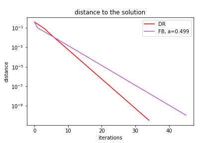
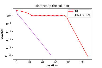
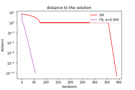
Figure 2: Comparison between DR and FB for the feasibility problem of a sphere and a line (seed=8). From left to right, n=2, 1000, 10000.

8.1.2 Inexact FB simulation

In this example, we exploit the inexact FB to find a point at the intersection of three circles and a line in $\mathbb{R}^{2}$. The inexact proximal calculation can be performed using Scipy’s built-in BFGS method to solve the smooth surrogate problem defined in Appendix E. All the calculations are done in Python with the Scipy package.

In this setting, we have $\mu=1$, $L_{g}=1$ and we consider $\rho=3$, so that inexactness parameter needs to satisfy the condition $\varepsilon<0.025$ – see (43). We test for various values of $\varepsilon\in\{0.0249,0.01,0.005,0.0025,0.001\}$ to analyse the algorithm’s behaviour depending on different levels of accuracy. Figure 3 (left) illustrates the configuration we considered along with the trajectories of the estimated sequences $x_{t}$ for different starting points $x_{0}$. Figure 3 (right) shows the distance from the iterates $x_{t}$ to the ground truth $x^{*}$ over 20000 iterations for $x_{0}=(5,5)$. All choices of $\varepsilon$ yield the same global behaviour for $\|x_{t}-x^{*}\|$, which monotonically decreases until a certain distance from the solution set is reached, exactly as stated in Theorem 1. Moreover, the convergence is faster as $\varepsilon$ becomes smaller: after five iterations, the sequence generated with $\varepsilon=0.001$ is approximately three orders of magnitude closer to the ground truth than the sequence generated with $\varepsilon=0.0249$.

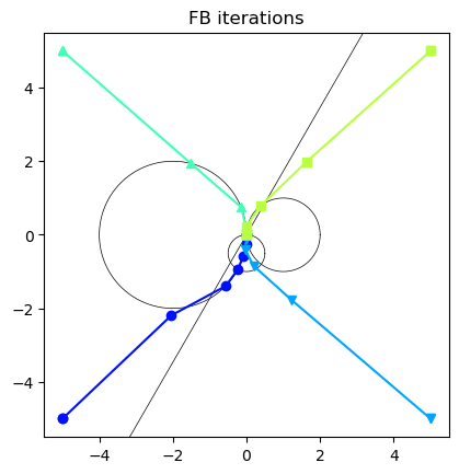
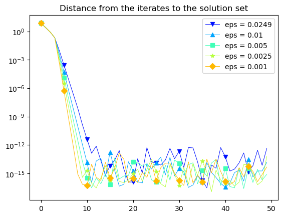
Figure 3: Feasibility problem between three circles and a line: Trajectories of the sequences generated at different starting points (left); distance from the iterates to the solution set for different levels of accuracy $\varepsilon$ (right).

9 Feasibility problem with separable functions

In this section we consider the Hilbert space $\mathcal{X}=\bigtimes_{i=1}^{n}\mathcal{X}_{i}$ where $\mathcal{X}_{i}$ is a Hilbert space, $i=1,\dots,n$. The inner product on $\mathcal{X}$ is defined as $\langle x\ |\ y\rangle=\sum\limits_{i=1}^{n}\langle x_{i}\ |\ y_{i}\rangle_{i}$ for $(x,y)\in\mathcal{X}\times\mathcal{X}$, and $\|\cdot\|_{\mathcal{X}}=\sqrt{\sum_{i=1}^{n}\|\cdot\|_{i}^{2}}$ where $\|\cdot\|_{i}$ is the norm of $\mathcal{X}_{i}$.

Phase retrieval and Source localization problems can be modelled by feasibility problems,

$$\text{find}\,x\in\bigcap\limits_{j=0}^{m}C^{j},$$ (92)

where each $C^{j}\subset\mathcal{X}_{i}$ is defined as $C^{j}:=\bigtimes_{i=1}^{n}C_{i}^{j}=\bigtimes_{i=1}^{n}\{x\in\mathcal{X}_{i}\,|\,\|x-c_{i}^{j}\|=r_{i}^{j}\}\subset\mathcal{X}_{i},$ for $m,n\in\mathbb{N}$ and given $c_{i}^{j}\in\mathcal{X}_{i},b^{j}_{i}\in(0,+\infty)$. The set $C^{0}\subset\mathcal{X}$ represents qualitative constraint and may be convex. See [41] for further details on this modelisation.

For $i=1,...,n$, $j=1,...,m$, a point $\overline{x}_{i}\in C_{i}^{j}$ if and only if $f_{i}^{j}(\overline{x}_{i})=0$, where ${f_{i}^{j}:\mathcal{X}_{i}\rightarrow[0,+\infty]}$,

$$\quad(\forall x_{i}\in\mathcal{X}_{i}) f_{i}^{j}(x)=|\|x_{i}-c_{i}^{j}\|^{2}_{i}-(r_{i}^{j})^{2}|.$$ (93)

The functions $f_{i}^{j}$, $i=1,...,n$, $j=1,...,m$, are $\rho$-weakly convex with $\rho=2$ and sharp with constant $\mu_{i}=1$ by analogous arguments as in Section 8. For $j=1,...,m$, let $F^{j}:\mathcal{X}\rightarrow[0,+\infty]$,

$$(\forall x\in\mathcal{X}) F^{j}(x):=\sum\limits_{i=1}^{n}f_{i}^{j}(x).$$ (94)

A point $\overline{x}\in C^{j}$ if and only if $F^{j}(\overline{x})=\sum\limits_{i=1}^{n}f_{i}(\overline{x}_{i})=0$ i.e.  $f_{i}^{j}(\overline{x})=0$, for all $i\in\{1,...,n\}$. The function $F^{j}$ is weakly convex and sharp thanks to its separable structure. The moduli of weak convexity and sharpness are inherited from $f_{i}^{j}$, which are $\rho=\rho_{i}$ and $\mu=\mu_{i}$.

Source Localization

For these problems, $m\leq 1000$, $n=1$ and $\mathcal{X}=\mathbb{R}^{2}$ or $\mathcal{X}=\mathbb{R}^{3}$ (we omit the index $"i"$). The aim is to locate the source of a signal, knowing the location $c_{j}$ of the $m$ sensors and the registered distance $r_{j}$. When the intersection is nonempty, problem (92) is equivalent to

$$\text{find}\ x\in\operatorname*{argmin}_{z\in C_{0}}\ F(x):=\sum\limits_{j=1}^{m}F^{j}(x)=\sum\limits_{j=1}^{m}|\|x-c^{j}\|^{2}-(r^{j})^{2}|,$$ (95)

where $F$ is weakly convex by Theorem 2. The problem (95) can be rewritten as the following feasibility problem

$$\operatorname*{argmin}_{x\in\mathcal{X}}\ \ F(x)+\frac{\operatorname{dist}^{2}(x,C_{0})}{2},$$ (FP1)

which is an instance of problem (2), when $C_{0}$ is convex.

In real-life source localization problems, measurements might be affected by a certain degree of uncertainty and we replace the function (94) in (95) with a function $\overline{F}^{j}:\mathcal{X}\times\mathbb{R}^{m}\rightarrow[0,+\infty]$,

$$(\forall(x,\delta)\in\mathcal{X}\times\mathbb{R}^{m}) \overline{F}^{j}(x,\delta):=\sum\limits_{j=1}^{m}\overline{f}^{j}(x,\delta^{j})=\sum\limits_{j=1}^{m}|\|x-c^{j}\|^{2}-(r^{j})^{2}-\delta^{j}|.$$ (96)

Function $\overline{F}^{j}$ is weakly convex and (globally) sharp, as we show in the following remark.

Remark 9.

Function $\overline{f}:\mathcal{X}\times\mathbb{R}\to\mathbb{R}$, with $f(x,y)=|\|x\|^{2}-y|$ is sharp. For every fixed $y\in(0,+\infty)$, we denote by $S(y)=\left\{w\in\mathcal{X}\,|\,{y}=\|w\|^{2}\right\}\subset\mathcal{X}$ the set of global minimisers of $\overline{f}(\cdot,y)$. By Lemma 8, for every $y\in[0,+\infty)$, $\overline{f}(\cdot,y)$ is sharp i.e. 

$$\left(\forall x\in\mathcal{X}\right)\qquad\qquad\overline{f}(x,y)\geq\operatorname{dist}(x,S(y)).$$

Moreover, the set $S(y)$ can be embedded into $\mathcal{X}\times[0,+\infty)$

$$S(y)\times\{y\}\subset\bigcup_{y\in[0,+\infty)}S(y)\times\{y\}=\{(x,y)\in\mathcal{X}\times[0,+\infty):\|x\|^{2}=y\}:=S$$ (97)

which is the set of global minimisers of $\overline{f}$. It then follows that

$$\left(\forall(x,y)\in\mathcal{X}\times[0,+\infty)\right) \overline{f}(x,y)\geq\operatorname{dist}(x,S(y))=\operatorname{dist}((x,y),S(y)\times\{y\})\geq\operatorname{dist}((x,y),S)$$ (98)

and the last inequality yields the sharpness of function $\overline{f}$. The same reasoning can be applied to prove the sharpness of the function $\overline{f}:\mathcal{X}\times\mathbb{R}\to\mathbb{R}$ $f(x,y)=|\|x-c\|^{2}-(y+r^{2})|$ for given $(c,r)\in\mathcal{X}\times\mathbb{R}$, which vanishes on the set $\left\{(x,y)\in\mathcal{X}\times\mathbb{R}\,|\,\|x-c\|^{2}=y+r^{2}\right\}\subset\mathcal{X}\times[-r^{2},+\infty)$.

The source localisation problem becomes

$$\text{find}\ (x,\delta)\in\operatorname*{argmin}_{(x,\delta)\in\mathcal{X}\times C_{0}}\ \overline{F}(x,\delta):=\sum\limits_{j=1}^{m}\overline{F}^{j}(x)=\sum\limits_{j=1}^{m}|\|x-c^{j}\|^{2}-(r^{j})^{2}-\delta^{j}|,$$ (99)

where the convex constraint $C_{0}:=\{\delta\in\mathbb{R}^{m}\ |\ \delta\in[\underline{\delta},\overline{\delta}]\},$ ensures that the exact location of the source is in the $\operatorname*{argmin}$ of (99). This is an advantage over other models with measurement uncertainty, where the optimal solution only approximates the true location of the source (see [8]).

Phase Retrieval

The problem is to recover the original signal affected by the measurement error $c_{i}^{j}$ from observation data $r_{i}^{j}$. The dimensions of the problem are $d=2,m$ ranges from $1$ to $10$ while $n$ can be up to $10000$. When $m=1$, we omit the index $"j"$ and the phase retrieval problem is equivalent to the feasibility problem of one sphere and a convex set in a product space. The phase retrieval problem for $m=1$ can be cast as

$$\underset{\begin{subarray}{c}{x\in\mathcal{X}}\end{subarray}}{\mathrm{minimize}}\;\;\,F(x)+\frac{\operatorname{dist}^{2}(x,C_{0})}{2}$$ (FP2)

and (FP2) can be solved by algorithm 1. In particular, since $F$ is a separable sum of functions of the form $f_{i}$, the proximity operator of $F$ is defined as

$$\quad(\forall y\in\mathcal{X}) \text{prox}_{\alpha F}(y)=\bigtimes_{i=1}^{n}\text{prox}_{\alpha f_{i}}(y^{i}),$$ (100)

where each $\text{prox}_{\alpha f_{i}}$ can be easily inferred from (90) in Example 4.

9.1 Inexact FB for source localization

We exploit the inexact FB to solve (99) to find the optimal solution of the source localization problem with measurement uncertainty [8, Example 1]. Here $\mathcal{X}=\mathbb{R}^{2}$. Starting from points generated with a pseudo-random uniform distribution and different seeds, we use the stopping criterion $\|(x,\varepsilon)_{n}-(x,\varepsilon)_{n+1}\|\leq 10^{-10}$. The exact solution is $(-2,3)$ and we show the approximated results obtained in [8].

Seed	Iteration Num.	Output
1	31	$(-2.0166,2.9687)$
3	26	$(-2.0414,2.9801)$

Method	R-LS	SDR	SR-LS	USR-LS
Output	$(-1.9907,3.0474)$	$(-1.7718,3.36655)$	$(-2.018,2.9585)$	$(-1.3450,2.6238)$

Table 1: First table: results with our approach for two different seeds. Second table: results from [8].

10 Discrete Tomography

Let $\mathcal{X}=\mathbb{R}^{n}$. Let us consider the function $F:\mathbb{R}^{n}\rightarrow\mathbb{R}$ defined as

$$\quad\left(\forall x\in\mathcal{X}\right) F({x})={\sum_{i=1}^{n}|x_{i}^{2}-1|},$$ (101)

which is the sum of functions $f_{i}^{j}$ from (93) for $j=1$, $\mathcal{X}_{i}=\mathbb{R}$, $c_{i}=0$ and $r_{i}=1$ for every $i=1,\dots,n$. By Lemma 8, $F$ is a (globally) sharp and weakly convex function with the set of minimisers ${S=\{x=(x_{1},\dots,x_{n})\in\mathbb{R}^{n}\,|\,x_{i}\in\{-1,1\}\;\text{for}\;i=1,\dots,n\}=\{-1,1\}^{n}}$, and can be seen as a non-smooth counterpart to the function ${x\mapsto{\sum_{i=1}^{n}x_{i}^{2}(x_{i}-1)^{2}}}$, $x\in\mathbb{R}^{n}$, proposed in [53] to promote binary integer solutions (with values in $\{0,1\}^{n}$) in Markov Random Field approaches. To the best of our knowledge, this is the first work where function $F$ is used in such a context.

Binary Tomography (BT) is a special case of Discrete Tomography (DT) which aims at reconstructing binary images starting from a limited number of their projections [48, 31]. The image $\overline{x}\in\mathbb{R}^{n}$ is represented as a grid of $n=n_{1}\times n_{2}$ pixels taking values $x_{j}\in\{-1,1\}$ for $j=1,\dots,n$. The projections $y_{i}$ for $i=1,\dots,m$ are linear combinations of the pixels along $m$ directions. The linear transformation from image to projections is modelled as

$$y=\mathbf{A}\overline{x}+\omega$$ (102)

where $x_{j}$ denotes the value of the image in the $j$-th cell, $y_{i}$ is the weighted sum of the image along the $i$-th ray, the element $\mathbf{A}_{i,j}$ of matrix $\mathbf{A}\in\mathbb{R}^{m\times n}$ is proportional to the length of the $i$-th ray in the $j$-th cell and finally $\omega\in\mathbb{R}^{n}$ is an additive noise with Gaussian distribution and standard deviation $\sigma>0$. In general, the projection matrix $\mathbf{A}$ has a low rank, meaning that $\operatorname{rank}(\mathbf{A})<\min\{n,m\}$ [31]. We cast the problem as

$$\text{Find}\quad x\in\{-1,1\}^{n}\quad\text{such\,that}\quad\|y-\mathbf{A}x\|_{2}\leq\theta$$ (103)

for some $\theta>0$, which can be reformulated as

$$\underset{\begin{subarray}{c}{{x\in{C}}}\end{subarray}}{\mathrm{minimize}}\;\;F(x)\quad\text{where}\quad{C}=\{x\in\mathbb{R}^{n}\,|\,\|\mathbf{A}x-y\|_{2}\leq\theta\}$$ (104)

with $F$ defined as in (101) and the constraint set ${C}$, represented by the function $\operatorname{dist}^{2}(\cdot,\overline{B}(y,\theta))/2$. In conclusion, we have

$$\underset{\begin{subarray}{c}{{x\in\mathbb{R}^{n}}}\end{subarray}}{\mathrm{minimize}}\;\;F(x)+\frac{\operatorname{dist}^{2}(\mathbf{A}x,\overline{B}(y,\theta))}{2}.$$ (105)

The sharpness of the objective function is ensured by Theorem 2, assuming that the set ${S}\cap C\neq\emptyset$ and equivalently $S\cap\operatorname*{argmin}\frac{\operatorname{dist}^{2}(\mathbf{A}x,\overline{B}(y,\theta))}{2}\neq\emptyset$ (for an adequate value of $\theta$, the original signal $\overline{x}$ belongs to the intersection). Clearly, for every $x\in\mathbb{R}^{n}$, $\iota_{\overline{B}(y,\theta)}(x)=\iota_{\overline{B}(0,\theta)}(x-y)$ and

$$\text{\rm proj}_{\overline{B}(y,\theta)}(x)=y+\text{\rm proj}_{\overline{B}(0,\theta)}(x-y)=y+\left((x-y)-\text{prox}_{\theta\|\cdot\|_{2}}(x-y)\right)=x-\text{prox}_{\theta\|\cdot\|_{2}}(x-y).$$ (106)

It follows that, by Lemma 9, for every $x\in\mathbb{R}^{n}$, $\nabla\left(\frac{\operatorname{dist}^{2}(\mathbf{A}x,\overline{B}(y,\theta))}{2}\right)=\mathbf{A}^{\top}\left(\text{prox}_{\theta\|\cdot\|_{2}}(\mathbf{A}x-y)\right)$ and $\|\mathbf{A}\|^{2}$ is a Lipschitz constant for this gradient.

Remark 10.

The model in (103) and (104) (for appropriate choices of matrix $\mathbf{A}\in\mathbb{R}^{m\times n}$, vector $y\in\mathbb{R}^{m}$ and possible additional convex constraints) could be applied to other Binary Quadratic Programs (a special class of QCQP problems having the equality constraint $x_{i}^{2}=1$ for every $i\in\{1,\dots,n\}$ ) arising in Computer Vision, such as Graph Bisection, Graph Matching and Image Co-Segmentation (see [52, Table 2] and the references therein).

Numerical tests

For our simulations we used the MATLAB codes and data from [31, 30]. We reproduced the same synthetic setting: we considered four phantoms (Apple, Lizard, Bell, Bird), corresponding to binary images of size 64 x 64 pixels. Operator $\mathbf{A}$ models an X-ray tomographic scan with 64 detectors and a parallel beam acquisition geometry with four angles (0°, 50°, 100°, 150°). We set $\sigma=0.01$ for the additive noise and $\theta=10(64\sigma)^{2}$ in the constraint set $\overline{B}(y,\theta)$. Figure 4 illustrates, from left to right, the original image and the reconstructions obtained with the Least Squares QR method (LSQR), with the Truncated Least Squares QR method (TLSQR), with the DUAL method proposed in [31] and finally with algorithm 1 applied to (105), which we refer to as Continuously Relaxed Binary Tomography (CRBT). All methods are initialised with a vector of zeros.

ccc ORIG	cci LSQR	cc TLSQR	cci DUAL	cciCRBT

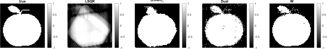
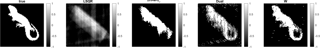
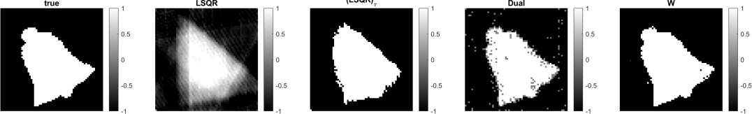
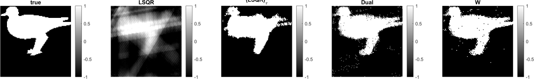
Figure 4: comparisons between different solutions. From left to right: original image, least squares solution, thresholded least squares solution, solution obtained with the dual method proposed in [31], solution obtained with our model.

11 Conclusions

We investigate the convergence properties of the exact and the inexact forward-backward algorithms for the minimisation of a function that is expressed as the sum of a weakly convex function and a smooth function with Lipschitz continuous gradient. In the inexact case, we inferred a convergence result that relies on the hypothesis that the accuracy level $\varepsilon>0$ for the inexact proximal computation is kept constant throughout all the iterations. We successfully applied the analysed method to feasibility problems in the context of source localisation and binary tomography. It will be interesting, in a future work, to extend our results so as to take into account non-constant accuracy levels $\varepsilon_{t}$.

Funding

This work was funded by the European Union’s Horizon 2020 research and innovation program under the Marie Skłodowska-Curie grant agreement No 861137. This work represents only the authors’ view and the European Commission is not responsible for any use that may be made of the information it contains.

Appendix A Proof of Proposition 6

The following theorem is inspired by [49, Theorem 5.2], originally in the finite-dimensional setting which can be easily adapted to the general Hilbert space setting.

Theorem 3.

Let $\mathcal{X}$ be a Hilbert space and $h:\mathcal{X}\rightarrow\mathbb{R}$ be a continuous $\rho$-weakly convex function, $h\geq 0$, $x^{*}\in S=\operatorname*{argmin}_{x\in\mathcal{X}}h(x)=[h\leq 0]\neq\emptyset$. Let $\delta_{0}>0$ and $r_{0}>0$. If there exists $\mu>0$ such that for every $x\in\overline{B}(x^{*},\delta_{0})\cap[0<h\leq r_{0}]$

$$\quad\left(\forall z\in\partial_{\rho}h(x)\right) \|z\|\geq\mu$$ (107)

then there exists $\eta>0$ such that for every $x\in{B}(x^{*},\eta)\cap[0<h<r_{0}]$

$$\ \ h(x)-h(x^{*})\geq\mu\ \operatorname{dist}(x,{S})$$ (108)

Proof of Proposition 6.

($(i)\implies(ii)$) We assume (28) holds for all ${x\in B(x^{*},\delta_{1})\cap[0<h(x)<r_{1}]}$. For any $0<\delta<\delta_{1}$ we consider $\overline{h}=h+\iota_{\overline{B}(x^{*},\delta)}$. By Lemma 3, we have

$$\inf_{x\in[0<\overline{h}<r_{1}]}\operatorname{dist}(\partial_{\rho/2}\overline{h}(x),0)=\inf_{0\leq r<r_{1}}\inf_{x\in[r<\overline{h}<r_{1}]}\frac{\overline{h}(x)-r}{\operatorname{dist}(x,[\overline{h}\leq r])}$$ (109)

For the RHS we have

$$\operatorname{RHS}=\inf_{0\leq r<r_{1}}\inf_{x\in[r<h<r_{1}]\cap\overline{B}(x^{*},\delta)}\frac{h(x)-r}{\operatorname{dist}(x,[h\leq r])}\geq\inf_{0\leq r<r_{1}}\inf_{x\in[r<h<r_{1}]\cap{B}(x^{*},\delta_{1})}\frac{h(x)-r}{\operatorname{dist}(x,[h\leq r])}$$ (110)

because $\overline{B}(x^{*},\delta)\subset{B}(x^{*},\delta_{1})$. On the other side, by [9, Theorem 2], the LHS is equivalent to

$$\operatorname{LHS}=\inf_{x\in[0<h<r_{1}]}\operatorname{dist}(\partial_{\rho/2}h(x)+N_{\overline{B}(x^{*},\delta)}x,0).$$ (111)

where $N_{\overline{B}(x^{*},\delta)}$ is the Normal Cone in the sense of convex analysis. For any $0<\delta_{2}<\delta$ and for any $0<r_{2}<r_{1}$ we have

$$\operatorname{LHS}\leq\inf_{x\in[0<h\leq r_{2}]\cap\overline{B}(x^{*},\delta_{2})}\operatorname{dist}(\partial_{\rho/2}h(x)+N_{\overline{B}(x^{*},\delta)}x,0)=\inf_{x\in[0<h\leq r_{2}]\cap\overline{B}(x^{*},\delta_{2})}\operatorname{dist}(\partial_{\rho/2}h(x),0)$$ (112)

where the last equality stems from the fact that $N_{\overline{B}(x^{*},\delta)}x=0$ for every $x\in B(x^{*},\delta)$. In conclusion we obtain

$$\inf_{x\in[0<h\leq r_{2}]\cap\overline{B}(x^{*},\delta_{2})}\operatorname{dist}(\partial_{\rho/2}h(x),0)\geq\inf_{0\leq r<r_{1}}\inf_{x\in[r<h<r_{1}]\cap{B}(x^{*},\delta_{1})}\frac{h(x)-r}{\operatorname{dist}(x,[h\leq r])}$$ (113)

and by (28) we get

$$\inf_{0\leq r<r_{1}}\inf_{x\in[r<h<r_{1}]\cap{B}(x^{*},\delta_{1})}\frac{h(x)-r}{\operatorname{dist}(x,[h\leq r])}\geq\mu>0,$$ (114)

which implies $\inf_{x\in[0<h\leq r_{2}]\cap\overline{B}(x^{*},\delta_{2})}\operatorname{dist}(\partial_{\rho/2}h(x),0)\geq\mu>0$, which is (29) with function $\varphi=\frac{1}{\mu}\operatorname{Id}$.

($(i)\implies(ii)$) The second part of the assertion follows from Theorem 3. ∎

Appendix B Proof of Lemma 4

Proof.

Take an arbitrary but fixed $t\in\mathbb{N}$ and let $\operatorname{dist}(x_{t+1},S)>0$. We take any $\overline{x}\in S$ and apply (34) from Proposition 7 for $x=\overline{x}$, which yields the following inequality:

$$(f+g)(\overline{x})-(f+g) (x_{t+1})\geq\left\langle\frac{x_{t}-x_{t+1}}{\alpha}\,|\,\overline{x}-x_{t+1}\right\rangle$$ (115)

$$-\frac{\rho}{2}\|\overline{x}-x_{t+1}\|^{2}-\frac{L_{g}}{2}\|x_{t}-x_{t+1}\|^{2}-\varepsilon-\sqrt{\frac{2\varepsilon}{\alpha}}\|\overline{x}-x_{t+1}\|.$$

By using the identity

$$\quad\left(\forall(w,y,z)\in\mathcal{X}^{3}\right) \left\langle w-y\,|\,y-z\right\rangle=\frac{1}{2}\|w-z\|^{2}-\frac{1}{2}\|w-y\|^{2}-\frac{1}{2}\|y-z\|^{2},$$

which follows from [6, Lemma 2.12], we obtain

$$\left(f+g\right)\left(\overline{x}\right)-\left(f+g\right)\left(x_{t+1}\right)\geq\frac{1}{2\alpha}\left(-\|x_{t}-\overline{x}\|^{2}+\|x_{t+1}-\overline{x}\|^{2}+\|x_{t}-x_{t+1}\|^{2}\right)$$ (116)

$$\qquad-\frac{\rho}{2}\left\|\overline{x}-x_{t+1}\right\|^{2}-\frac{L_{g}}{2}\left\|x_{t}-x_{t+1}\right\|^{2}-\varepsilon-\sqrt{\frac{2\varepsilon}{\alpha}}\left\|\overline{x}-x_{t+1}\right\|$$

$$\qquad=\left(\frac{1}{2\alpha}-\frac{L_{g}}{2}\right)\|x_{t}-x_{t+1}\|^{2}+\left(\frac{1}{2\alpha}-\frac{\rho}{2}\right)\left\|\overline{x}-x_{t+1}\right\|^{2}-\frac{1}{2\alpha}\|x_{t}-\overline{x}\|^{2}-\varepsilon-\sqrt{\frac{2\varepsilon}{\alpha}}\left\|\overline{x}-x_{t+1}\right\|.$$

Using Young’s Inequality, we have

$$-\sqrt{\frac{2\varepsilon}{\alpha}}\left\|\overline{x}-x_{t+1}\right\|\geq-\frac{1}{2}\|\overline{x}-x_{t+1}\|^{2}-\frac{\varepsilon}{\alpha}.$$ (117)

Plugging (117) back into (116) yields

$$\qquad\qquad\left(f+g\right)\left(\overline{x}\right)-\left(f+g\right)\left(x_{t+1}\right)\geq$$ (118)

$$\left(\frac{1}{2\alpha}-\frac{L_{g}}{2}\right)\|x_{t}-x_{t+1}\|^{2}+\left(\frac{1}{2\alpha}-\frac{\rho+1}{2}\right)\left\|\overline{x}-x_{t+1}\right\|^{2}-\frac{1}{2\alpha}\|x_{t}-\overline{x}\|^{2}-\frac{\alpha+1}{\alpha}\varepsilon.$$

We then estimate the LHS of (118) by the assumption of sharpness on $f+g$

$$-\mu\operatorname{dist}(x_{t+1},S) \geq\left(\frac{1}{2\alpha}-\frac{\rho+1}{2}\right)\left\|\overline{x}-x_{t+1}\right\|^{2}-\frac{1}{2\alpha}\|x_{t}-\overline{x}\|^{2}+\left(\frac{1}{2\alpha}-\frac{L_{g}}{2}\right)\|x_{t}-x_{t+1}\|^{2}-\frac{\alpha+1}{\alpha}\varepsilon.$$

By using (44) from Assumption 2 and the fact that $\overline{x}\in S$ can be taken arbitrarily, we choose $\overline{x}\in S$ so that

$$\|x_{t}-\overline{x}\|^{2}\geq\operatorname{dist}^{2}(x_{t},S)\qquad\text{and}\qquad\|x_{t+1}-\overline{x}\|^{2}\geq\operatorname{dist}^{2}(x_{t+1},S)$$

which yields

$$-\mu\operatorname{dist}(x_{t+1},S) \geq\left(\frac{1}{2\alpha}-\frac{\rho+1}{2}\right)\operatorname{dist}^{2}(x_{t+1},S)-\frac{1}{2\alpha}\operatorname{dist}^{2}(x_{t},S)-\frac{\alpha+1}{\alpha}\varepsilon$$

$$\begin{split}\iff\operatorname{dist}^{2}(x_{t},S)\geq\left(1-\alpha\rho-\alpha\right)\operatorname{dist}^{2}(x_{t+1},S)+2\alpha\mu\operatorname{dist}(x_{t+1},S)-2(\alpha+1)\varepsilon\end{split}$$ (119)

Let now $t=t_{0}$. By hypothesis (49), we have

$$\left(1-\alpha\rho-\alpha\right)\text{dist}^{2}\left(x_{t+1},S\right)+2\alpha\mu\text{dist}\left(x_{t+1},S\right)-2(\alpha+1)\varepsilon\leq(E^{+})^{2}$$ (120)

which is a second degree inequality with respect $\operatorname{dist}(x_{t+1},S)$. he discriminant has the form

$$\Delta=\left(\frac{\mu+\left(1-\alpha\left(\rho+1\right)\right)\sqrt{\mu^{2}-2\varepsilon\left(\rho+1\right)\frac{\alpha+1}{\alpha}}}{1+\rho}\right)^{2}\geq 0.$$ (121)

Since $\Delta\geq 0$, the solutions are within the following range

$$\frac{-\alpha\mu-\sqrt{\Delta}}{1-\alpha\rho-\alpha} \leq\operatorname{dist}\left(x_{t+1},S\right)\leq\frac{-\alpha\mu+\sqrt{\Delta}}{1-\alpha\rho-\alpha}=\frac{\mu+\sqrt{\mu^{2}-2\varepsilon\left(\rho+1\right)\frac{\alpha+1}{\alpha}}}{1+\rho}=E^{+}$$ (122)

In conclusion, since the distance from a set is a non-negative value, we obtain

$$0\leq\operatorname{dist}\left(x_{t+1},S\right)\leq E^{+}.$$ (123)

which by induction proves (49). The same reasoning can be applied to obtain (50). ∎

Appendix C Proof of Lemma 5

Proof of Lemma 5.

The quantities $E^{+}$ and $E^{-}$ are roots of the quadratic equation

$$(E^{-})^{2}=(1-\alpha\rho-\alpha)(E^{-})^{2}+2\alpha\mu E^{-}-2(\alpha+1)\varepsilon.$$ (124)

Subtracting (124) from (119), we obtain the following inequality that holds for every $t\in\mathbb{N}$

$$\operatorname{dist}^{2}(x_{t},S)-(E^{-})^{2}\geq$$ (125)

$$(1-\alpha\rho-\alpha)(\operatorname{dist}^{2}(x_{t+1},S)-(E^{-})^{2})+2\alpha\mu(\operatorname{dist}(x_{t+1},S)-E^{-})+(1-\alpha L_{g})\|x_{t}-x_{t+1}\|^{2}$$

$$=(1-\alpha\rho-\alpha+\frac{2\alpha\mu}{\operatorname{dist}(x_{t+1},S)+E^{-}})\left(\operatorname{dist}^{2}(x_{t+1},S)-(E^{-})^{2}\right)+(1-\alpha L_{g})\|x_{t}-x_{t+1}\|^{2}.$$

Then,

$$\operatorname{dist}^{2}(x_{t},S)-(E^{-})^{2}\geq\zeta_{{t}+1}\left(\operatorname{dist}^{2}(x_{t+1},S)-(E^{-})^{2}\right)+(1-\alpha L_{g})\|x_{t}-x_{t+1}\|^{2},$$ (126)

where ${\zeta_{t+1}:=1-\alpha\rho-\alpha+\dfrac{2\alpha\mu}{\operatorname{dist}(x_{t+1},S)+E^{-}}\geq 0}$ is non-negative by Assumption 2. By dropping the term $(1-\alpha L_{g})\|x_{t}-x_{t+1}\|^{2}$ (positive by (44)), we have

$$\operatorname{dist}^{2}(x_{t},S)-(E^{-})^{2}\geq\zeta_{{t}+1}\left(\operatorname{dist}^{2}(x_{t+1},S)-(E^{-})^{2}\right).$$ (127)

Now we show that at iteration $t\geq t_{0}$, we have $\zeta_{t+1}\geq 1$. Notice that $\zeta_{t+1}\geq 1$ whenever $\frac{2\alpha\mu}{\operatorname{dist}(x_{t+1},S)+E^{-}}\geq\alpha\rho+\alpha.$ Equivalently,

$$\operatorname{dist}(x_{t+1},S) \leq\frac{2\mu}{\rho+1}-E^{-}=\frac{\mu+\sqrt{\mu^{2}-2\varepsilon(\rho+1)\frac{\alpha+1}{\alpha}}}{\rho+1}=E^{+}.$$ (128)

By assumption, there exists $t_{0}$ such that $\operatorname{dist}(x_{t_{0}},S)\leq E^{+}$ and, by Lemma 4, this implies that ${\operatorname{dist}(x_{t+1},S)\leq E^{+}}$. In conclusion, for every $t\geq t_{0}$ the condition $\zeta_{t+1}\geq 1$ holds. ∎

Appendix D Proof of Lemma 8

Proof.

For $x\in\mathcal{X}$, the distance to the sphere $\mathcal{S}$ is given as ${x}\mapsto{|\|x\|-1|}$. We show that for $\mu=1$ we have

$$\quad(\forall x\in\mathcal{X}) |\|x\|^{2}-1|\geq\mu\operatorname{dist}(x,S).$$

If $x=0$, then $\operatorname{dist}(x,\mathcal{S})=1$ and the inequality is satisfied for $\mu=1$. Otherwise, for every $x\in\mathcal{X}\setminus 0$ we have

$$\min_{s\in\mathcal{S}}\|x-s\|=\|x-\frac{x}{\|x\|}\|=\|x\left(1-\frac{1}{\|x\|}\right)\|=\|x\|\left|1-\frac{1}{\|x\|}\right|=\|x\|\frac{1}{\|x\|}\left|\|x\|-1\right|=|\|x\|-1|.$$

Consider $\tilde{f}:\mathbb{R}\rightarrow\mathbb{R}$ defined as ${\sigma\mapsto|\sigma^{2}-1|}$, i.e.  the function from Example 1 with $(a,b)=(-1,1)$. The following inequality is satisfied for every $\delta\leq 1$ (as illustrated in Figure 1)

$$\quad(\forall\sigma\in\mathbb{R}) \delta||\sigma|-1|=\delta\min\{|\sigma-1|,|\sigma+1|\}\leq|\sigma^{2}-1|.$$

where the last inequality holds by the sharpness of function $\tilde{f}$ (see Example 2). Choosing $\sigma=\|x\|$ we obtain

$$\quad(\forall x\in\mathcal{X}\setminus 0) \delta|\|x\|-1|\leq|\|x\|^{2}-1|.$$

Thus, $\mu\operatorname{dist}(x,\mathcal{S})\leq f(x)$, for $\mu\in(0,1]$, for $x\in\mathcal{X}$ which implies the global sharpness of $f$ with $\mu=1$. ∎

Appendix E Inexact Proximal Computation

For any strongly convex function $h$ and its unique minimiser $\overline{x}$,

$$\operatorname{lev}_{\leq\varepsilon+h(\overline{x})}h:=\{x\in\mathcal{X}\,|\,h(x)\leq\varepsilon+h(\overline{x})\}$$ (129)

is the set of $\varepsilon$-solutions of $h$. If, for some $y\in\mathcal{X}$, and $f$ $\rho$-weakly convex with $\alpha<\frac{1}{\rho}$, for every $x\in\mathcal{X}$, function $h$ is defined as ${h(x):=f(x)+\frac{1}{2\alpha}\|x-y\|^{2}}$, then $\varepsilon\operatorname{-prox}_{\alpha f}(y)=\operatorname{lev}_{\leq\varepsilon+h(\overline{x})}h$, where $\overline{x}$ is the exact proximal point of $f$ at $y$.

Lemma 10.

Let $h,\,\widehat{h}:\mathcal{X}\rightarrow(-\infty,+\infty]$ be two strongly convex functions with minimisers $\overline{x}\in\mathcal{X}$ and $\widehat{x}\in\mathcal{X}$ respectively. Assume that for every $\varepsilon\geq 0$

$$(\forall x\in\mathcal{X})\qquad\qquad h(x)\leq\widehat{h}(x)\leq h(x)+\varepsilon.$$ (130)

Then, the unique minimiser $\widehat{x}$ of $\widehat{h}$ belongs to $\operatorname{lev}_{\leq\varepsilon+h(\overline{x})}h$.

Proof.

By contradiction, assume that $\widehat{x}\notin\operatorname{lev}_{\leq\varepsilon+h(\overline{x})}h$, i.e. , $h(\widehat{x})>\varepsilon+h(\overline{x}).$ By assumption, for $x=\widehat{x}$, equation (130) reads as $h(\widehat{x})\leq\widehat{h}(\widehat{x})\leq h(\widehat{x})+\varepsilon$ which combined with our hypothesis implies $\varepsilon+h(\overline{x})<\widehat{h}(\widehat{x}).$ On the other side, for $x=\overline{x}$, equation (130) reads as $h(\overline{x})\leq\widehat{h}(\overline{x})\leq h(\overline{x})+\varepsilon$, which implies $\widehat{h}(\overline{x})\leq\varepsilon+h(\overline{x}).$ This induces $\widehat{h}(\overline{x})\leq\varepsilon+h(\overline{x})<\widehat{h}(\widehat{x})$ which is a contradition because $\widehat{x}$ is the unique minimiser of $\widehat{h}$. ∎

Example 5.

Let $(a_{1},\dots,a_{n}),(b_{1},\dots,b_{n})\in\mathbb{R}^{n}$ be pair of vectors. The function $F:\mathbb{R}\rightarrow\mathbb{R}$ defined, for every $x\in\mathbb{R}^{n}$, as $F(x):=\sum_{i=1}^{n}|(x-a_{i})(x-b_{i})|$ lacks an explicit formula for its proximal operator. Consider the function $\widehat{F}:\mathbb{R}^{n}\rightarrow\mathbb{R}$ defined, for every $x\in\mathbb{R}^{n}$ as $\widehat{F}(x)=\sum_{i=1}^{n}\sqrt{((x-a_{i})(x-b_{i}))^{2}+\varepsilon_{i}^{2}}$ for given $\varepsilon_{i}>0$, $i=1,\dots,n$. It is easy to see that for every $x\in\mathbb{R}^{n}$

$$F(x)\leq\widehat{F}(x)\leq\sum_{i=1}^{n}\left(|((x-a_{i})(x-b_{i}))|+\varepsilon_{i}\right)\leq F(x)+\sum_{i=1}^{n}\varepsilon_{i}.$$ (131)

Functions $h:=F+\frac{1}{2\alpha}\|\cdot-y\|^{2}$ and $\widehat{h}:=\widehat{F}+\frac{1}{2\alpha}\|\cdot-y\|^{2}$ satisfy (130) with $\varepsilon=\sum_{i=1}^{n}\varepsilon_{i}$ and by solving the surrogate smooth and strongly convex problem

$$\operatorname*{argmin}_{x\in\mathbb{R}^{n}}\widehat{F}(x)+\frac{1}{2\alpha}\|x-y\|^{2}$$ (132)

we obtain a point in $\varepsilon\operatorname{-prox}_{\alpha F}(y)$. In particular, solving (132) corresponds to solving $n$ independent smooth and strongly convex 1-dimensional problems.

References

- [1] Atenas, F., Sagastizàbal, C., Silva, P. J. S., and Solodov, M. A unified analysis of descent sequences in weakly convex optimization, including convergence rates for bundle methods. SIAM Journal on Optimization 33, 1 (2023), 89–115.
- [2] Attouch, H., Bolte, J., and Svaiter, B. F. Convergence of descent methods for semi-algebraic and tame problems: proximal algorithms, forward–backward splitting, and regularized Gauss–Seidel methods. Mathematical Programming 137, 1 (2013), 91–129.
- [3] Azé, D., and Corvellec, J.-N. Characterizations of error bounds for lower semicontinuous functions on metric spaces. ESAIM: Control, Optimisation and Calculus of Variations 10, 3 (2004), 409–425.
- [4] Bai, S., Li, M., Lu, C., Zhu, D., and Deng, S. The equivalence of three types of error bounds for weakly and approximately convex functions. Journal of Optimization Theory and Applications (03 2022), 1–26.
- [5] Barré, M., Taylor, A. B., and Bach, F. Principled analyses and design of first-order methods with inexact proximal operators. Mathematical Programming (2022), 1–46.
- [6] Bauschke, H. H., and Combettes, P. L. Convex Analysis and Monotone Operator Theory in Hilbert Spaces, 2nd ed. Springer Publishing Company, Incorporated, 2017.
- [7] Bayram, I. On the convergence of the iterative shrinkage/thresholding algorithm with a weakly convex penalty. IEEE Transactions on Signal Processing 64, 6 (2015), 1597–1608.
- [8] Beck, A., Stoica, P., and Li, J. Exact and approximate solutions of source localization problems. IEEE Transactions on signal processing 56, 5 (2008), 1770–1778.
- [9] Bednarczuk, E., Bruccola, G., Scrivanti, G., and Tran, T. H. Calculus rules for proximal -subdifferentials and inexact proximity operators for weakly convex functions. In 2023 European Control Conference (ECC) (2023).
- [10] Bello-Cruz, Y., Gonçalves, M. L., and Krislock, N. On fista with a relative error rule. Computational Optimization and Applications (2022), 1–24.
- [11] Benoist, J. The douglas–rachford algorithm for the case of the sphere and the line. Journal of Global Optimization 63 (2015), 363–380.
- [12] Bernard, F., and Thibault, L. Prox-regular functions in Hilbert spaces. Journal of Mathematical Analysis and Applications 303, 1 (2005), 1–14.
- [13] Böhm, A., and Wright, S. J. Variable smoothing for weakly convex composite functions. Journal of optimization theory and applications 188, 3 (2021), 628–649.
- [14] Bolte, J., Daniilidis, A., Ley, O., and Mazet, L. Characterizations of Łojasiewicz inequalities and applications. Transactions of the American Mathematical Society 362, 6 (2010), 3319–3363.
- [15] Bolte, J., Sabach, S., and Teboulle, M. Proximal alternating linearized minimization for nonconvex and nonsmooth problems. Mathematical Programming 146, 1-2 (2014), 459–494.
- [16] Bonettini, S., Loris, I., Porta, F., Prato, M., and Rebegoldi, S. On the convergence of a linesearch based proximal-gradient method for nonconvex optimization. Inverse Problems 33, 5 (2017), 055005.
- [17] Bonettini, S., Ochs, P., Prato, M., and Rebegoldi, S. An abstract convergence framework with application to inertial inexact forward–backward methods. Computational Optimization and Applications (2023), 1–44.
- [18] Borwein, J. M., and Sims, B. The Douglas–Rachford algorithm in the absence of convexity. Fixed-point algorithms for inverse problems in science and engineering (2011), 93–109.
- [19] Burke, J. V., and Ferris, M. C. Weak sharp minima in mathematical programming. SIAM Journal on Control and Optimization 31, 5 (1993), 1340–1359.
- [20] Cannarsa, P., and Sinestrari, C. Semiconcave functions, Hamilton-Jacobi equations, and optimal control, vol. 58. Springer Science & Business Media, 2004.
- [21] Chierchia, G., Chouzenoux, E., Combettes, P. L., and Pesquet, J.-C. The proximity operator repository. http://proximity-operator.net/index.html.
- [22] Clarke, F. H., Ledyaev, Y. S., Stern, R. J., and Wolenski, P. R. Nonsmooth analysis and control theory, vol. 178. Springer Science & Business Media, 2008.
- [23] Combettes, P. L., and Vũ, B. C. Variable metric forward–backward splitting with applications to monotone inclusions in duality. Optimization 63, 9 (2014), 1289–1318.
- [24] Combettes, P. L., and Wajs, V. R. Signal recovery by proximal forward-backward splitting. Multiscale modeling & simulation 4, 4 (2005), 1168–1200.
- [25] Davis, D., and Drusvyatskiy, D. Stochastic model-based minimization of weakly convex functions. SIAM Journal on Optimization 29, 1 (2019), 207–239.
- [26] Davis, D., Drusvyatskiy, D., MacPhee, K. J., and Paquette, C. Subgradient methods for sharp weakly convex functions. Journal of Optimization Theory and Applications 179, 3 (2018), 962–982.
- [27] Guan, W.-B., and Song, W. The forward–backward splitting method for non-Lipschitz continuous minimization problems in banach spaces. Optimization Letters 16, 8 (2022), 2435–2456.
- [28] Han, S.-P., and Lou, G. A parallel algorithm for a class of convex programs. SIAM Journal on Control and Optimization 26, 2 (1988), 345–355.
- [29] Jourani, A. Subdifferentiability and subdifferential monotonicity of -paraconvex functions. Control and Cybernetics 25 (1996).
- [30] Kadu, A. Binarytomo toolbox. https://github.com/ajinkyakadu/BinaryTomo.
- [31] Kadu, A., and van Leeuwen, T. A convex formulation for binary tomography. IEEE Transactions on Computational Imaging 6 (2020), 1–11.
- [32] Kruger, A. Y., López, M. A., Yang, X., and Zhu, J. Hölder error bounds and Hölder calmness with applications to convex semi-infinite optimization. Set-Valued and Variational Analysis (2019), 1–29.
- [33] Kurdyka, K. On gradients of functions definable in o-minimal structures. Annales de l’Institut Fourier 48, 3 (1998), 769–783.
- [34] Li, X., Chen, S., Deng, Z., Qu, Q., Zhu, Z., and Man-Cho So, A. Weakly convex optimization over stiefel manifold using riemannian subgradient-type methods. SIAM Journal on Optimization 31, 3 (2021), 1605–1634.
- [35] Li, X., Zhu, Z., So, A. M.-C., and Lee, J. D. Incremental methods for weakly convex optimization. arXiv preprint arXiv:1907.11687 (2019).
- [36] Lions, P.-L., and Mercier, B. Splitting algorithms for the sum of two nonlinear operators. SIAM Journal on Numerical Analysis 16, 6 (1979), 964–979.
- [37] Liu, T., and Pong, T. K. Further properties of the forward–backward envelope with applications to difference-of-convex programming. Computational Optimization and Applications 67 (2017), 489–520.
- [38] Łojasiewicz, S. Une propriété topologique des sous-ensembles analytiques réels. Equ. Derivees partielles, Paris 1962, Colloques internat. Centre nat. Rech. sci. 117, 87-89 (1963)., 1963.
- [39] Łojasiewicz, S. Sur la géométrie semi- et sous- analytique. Annales de l’Institut Fourier 43, 5 (1993), 1575–1595.
- [40] Lorenz, D. A., and Pock, T. An inertial forward-backward algorithm for monotone inclusions. Journal of Mathematical Imaging and Vision 51, 2 (2015), 311–325.
- [41] Luke, D. R., Sabach, S., and Teboulle, M. Optimization on spheres: models and proximal algorithms with computational performance comparisons. SIAM Journal on Mathematics of Data Science 1, 3 (2019), 408–445.
- [42] Millán, R., and Penton, M. Inexact proximal -subgradient methods for composite convex optimization problems. Journal of Global Optimization 75 (2019).
- [43] Polyak, B. Sharp minima, 1979. Institute of Control Sciences lecture notes, Moscow, USSR, In IIASA workshop on generalized Lagrangians and their applications, IIASA, Laxenburg, Austria, 1979.
- [44] Rockafellar, R., and Wets, R. J.-B. Variational Analysis. Springer Verlag, Heidelberg, Berlin, New York, 1998.
- [45] Rolewicz, S. On paraconvex multifunctions. Oper. Res.-Verf. 31 (1979), 539–546.
- [46] Rolewicz, S. On a globalization property. Applicationes Mathematicae 22, 1 (1993), 69–73.
- [47] Salzo, S., and Villa, S. Inexact and accelerated proximal point algorithms. Journal of Convex Analysis 19, 4 (2012), 1167–1192.
- [48] Schüle, T., Schnörr, C., Weber, S., and Hornegger, J. Discrete tomography by convex–concave regularization and d.c. programming. Discrete Applied Mathematics 151, 1 (2005), 229–243. IWCIA 2003-Ninth International Workshop on Combinatorial Image Analysis.
- [49] Studniarski, M., and Ward, D. E. Weak sharp minima: characterizations and sufficient conditions. SIAM Journal on Control and Optimization 38, 1 (1999), 219–236.
- [50] Vial, J.-P. Strong and weak convexity of sets and functions. Mathematics of Operations Research 8, 2 (1983), 231–259.
- [51] Villa, S., Salzo, S., Baldassarre, L., and Verri, A. Accelerated and inexact forward-backward algorithms. SIAM Journal on Optimization 23, 3 (2013), 1607–1633.
- [52] Wang, P., Shen, C., Hengel, A. v. d., and Torr, P. H. S. Large-scale binary quadratic optimization using semidefinite relaxation and applications. IEEE Transactions on Pattern Analysis and Machine Intelligence 39, 3 (2017), 470–485.
- [53] Yang, X., and Liu, Z.-Y. A doubly graduated method for inference in markov random field. SIAM Journal on Imaging Sciences 14, 3 (2021), 1354–1373.