Multi-Task Reinforcement Learning in Continuous Control with Successor Feature-Based Concurrent Composition

Abstract

Deep reinforcement learning (DRL) frameworks are increasingly used to solve high-dimensional continuous-control tasks in robotics. However, due to the lack of sample efficiency, applying DRL for online learning is still practically infeasible in the robotics domain. One reason is that DRL agents do not leverage the solution of previous tasks for new tasks. Recent work on multi-tasking DRL agents based on successor features has proven to be quite promising in increasing sample efficiency. In this work, we present a new approach that unifies two prior multi-task RL frameworks, SF-GPI and value composition, for the continuous control domain. We exploit compositional properties of successor features to compose a policy distribution from a set of primitives without training any new policy. Lastly, to demonstrate the multi-tasking mechanism, we present a new benchmark for multi-task continuous control environment based on Raisim. This also facilitates large-scale parallelization to accelerate the experiments. Our experimental results in the Pointmass environment show that our multi-task agent has single task performance on par with soft actor critic (SAC) and the agent can successfully transfer to new unseen tasks where SAC fails. We provide our code as open-source at https://github.com/robot-perception-group/concurrent_composition for the benefit of the community.

I Introduction

One approach to achieve optimal continuous control in robotics is through reinforcement learning-based methods (RL) [1]. However, RL agents are usually optimized for one specific task and require more training if the reward definition changes. On the other hand, multi-task RL frameworks aim to design an RL agent that allows recycling old policies for other tasks to achieve higher sample efficiency[2].

One way to achieve multi-task RL is through transfer learning by manipulating the policies trained on the old tasks. In this work, we focus on the transfer learning methods that define tasks using linearly decomposable reward functions, commonly used to define many robot control tasks [3].

Figure 1: In concurrent composition, policy extraction is too expensive to perform in every time step. Instead, we propose composing the primitives directly in the run time.

Currently, there are two major transfer learning frameworks following the aforementioned assumption. The first framework, using successor features and generalized policy improvement (SF-GPI, [4, 5]), derives the new policy by choosing the sub-policies, or primitives, with the largest associated action-value. The other framework directly composes the action-value of different tasks, which we refer to as value composition (VC [6, 7, 8, 9]). This framework first defines the composite value functions of new tasks by linearly combining the constituent action-value functions and then extracts the policy.

Different from the Option framework[10], which is an another approach to multi-task RL that combines the primitives in temporal order, in our novel approach we focus on concurrent policy composition by composing the primitives at every time step. The samples collected by the composite policy expose each primitive to a higher quality data and thus enable the knowledge transfer and increase the sample efficiency [4]. Policy extraction is prohibitive since it requires updating policies multiple times. We consider real-time performance as critical. Therefore, we must adapt VC-based methods for online composition. We do so by multiplicative policy composition (MCP [11]). We show that this can be achieved via the successor features framework, where SF-GPI becomes one special case.

In summary our contributions include the following.

• Derivation of the relation between value composition and policy composition.

• A novel method unifying the GPI and VC under the successor feature-based online concurrent composition framework.

• Introduction of a new benchmark environment based on Raisim for multi-task reinforcement learning.

II Related work

The compositional agents in our framework build upon the two transfer learning frameworks: VC and SF-GPI. VC-based methods mainly came from the maximum entropy framework[12]. By encouraging policy randomness, the resulting policy is usually more robust against the noise [13] and exhibits better exploratory behavior[14]. The value composition methods often exploit the property that the optimal value function of conjunction tasks can be well approximated by the average of the constituent value functions [6, 7]. Interestingly, boolean operators can further expand the valid compositions in the discrete setting and achieve a super-exponential amount of task transfer[8, 9]. However, none of these approaches consider concurrent composition scenarios.

On the other hand, SF-GPI[4] applies successor features [15] to estimate a set of Q-functions. Maximizing these Q-functions results in the policy improvement. The results in [4] indicate that training several primitives simultaneously can significantly improve the sample efficiency more than training individually. Our work can be seen as an extension to SF-GPI by bringing valid operations from VC to successor feature-enabled concurrent learning.

III Background

III-A Multi-Task Reinforcement Learning

RL improves a control policy through interaction with the environment, and it formulates this procedure by Markov decision processes (MDPs), $\mathcal{M}\equiv<\mathcal{S},\mathcal{A},p,r,\gamma>$. $\mathcal{S}$ and $\mathcal{A}$ define the state space and action space respectively. The dynamics $p(s_{t+1}|s_{t},a_{t})$ defines the transition probability from one state to another. Reward function $r(s_{t},a_{t},s_{t+1})$ governs the desired agent behavior. The discount $\gamma\in[0,1)$ determines the valid time horizon of the task. The goal is to find the optimal control policy $\pi(a|s):S\rightarrow A$, such that the expected discounted return, $J(\pi)=\mathbb{E}_{\pi,\mathcal{M}}[\sum_{\tau=t}^{\infty}\gamma^{\tau-t}r_{\tau}]$, can be maximized.

We consider transfer within a set of MDPs $\mathcal{M}_{w}\in\mathcal{T}$ where $\mathcal{M}_{w}\equiv<\mathcal{S},\mathcal{A},p,r_{w},\gamma>$ , and each has its unique reward function, $r_{w}(s_{t},a_{t},s_{t+1})=\phi(s_{t},a_{t},s_{t+1})^{\top}\cdot w$, which is a linear combination of a set of commonly shared $d$ features, $\phi(s_{t},a_{t},s_{t+1})\in\mathbb{R}^{d}$ and the task weight $w\in\mathbb{R}^{d}$. The goal is to find a set of primitives that can solve the subset of tasks $\mathcal{T}^{\prime}\in\mathcal{T}$ such that we can recover the optimal policies from the unseen tasks by the found primitives.

III-B Maximum Entropy RL

The maximum RL framework includes a bonus policy entropy term in the expected reward function. The goal is to find an optimal control policy that not only maximizes the reward but also encourages the policy randomness,

$$J(\pi)=\mathbb{E}_{\pi,\mathcal{M}_{w}}\left[\sum_{\tau=t}^{\infty}\gamma^{\tau-t}(r_{w,\tau}+\alpha\mathcal{H}(\pi(\cdot|s_{\tau})))\right],$$ (1)

where $\alpha$ is a temperature scaler controlling the entropy of the policy and $\mathcal{H}(\cdot)$ is an entropy estimator. Prior works have found that the bonus term can encourage exploration [16], increase the training policy’s robustness against noise [13], and preserve the policy multimodality [14].

One tractable way to achieve maximum entropy RL is through temporal difference learning by boostrapping the value estimation. Here, we define the action-value function, or Q-function, of policy $\pi$ on task $w$ as:

$$Q^{\pi}_{w}(s_{t},a_{t})\equiv r_{w,t}+\mathbb{E}_{\pi}\left[\sum_{\tau=t+1}^{\infty}\gamma^{\tau-t}(r_{w,\tau}+\alpha\mathcal{H}(\pi(\cdot|s_{\tau})))\right].$$ (2)

Note when $\alpha=0$, we recover the standard RL Q-function. The Q-function can be perceived as a performance metric of its policy and the estimation quality can be improved recursively through the soft policy iteration.

III-C Soft Policy Iteration

The soft policy iteration can be defined in two steps: (1) soft policy evaluation (2) soft policy improvement [14]. The soft policy evaluation step allows to improve the quality of Q-value estimation and it can be formulated as follows,

$$Q^{\pi}_{w}(s_{t},a_{t}) =r_{w}(s_{t},a_{t})+\gamma\mathbb{E}_{s_{t+1}\sim p}\left[V(s_{t+1})\right]$$ (3)

$$V^{\pi}_{w}(s_{t}) =\mathbb{E}_{a_{t}\sim\pi}\left[Q^{\pi}_{w}(s_{t},a_{t})-\log\pi(a_{t}|s_{t})\right].$$ (4)

The policy distribution can be updated according to the soft policy improvement step:

$$\pi_{new}=\operatorname*{\arg\!\min}_{\pi^{\prime}}D_{KL}\left(\pi^{\prime}(\cdot|s_{t})||\frac{\exp(Q^{\pi_{old}}_{w}(s_{t},\cdot))}{Z^{\pi_{old}}(s_{t})}\right),$$ (5)

where $D_{KL}$ denotes the Kullback-Leiber divergence and the normalizing factor, $Z^{\pi_{old}}(s_{t})$, can be neglected because it does not contribute to the gradient computation. Intuitively, the goal is to match the policy distribution to the Q-value estimation of different actions; therefore, the higher the Q-value, the higher the probability of selecting the action, i.e.

$$\pi(\cdot|s)\propto e^{Q^{\pi}(s,\cdot)}.$$ (6)

Alternating between the policy evaluation step and policy improvement step will eventually converge to the optimal Q-function $Q^{*}_{w}$ on task $w$ with its corresponding optimal policy $\pi^{*}$, where $Q^{*}_{w}\equiv Q^{\pi^{*}}_{w}$ [14].

III-D Successor Feature (SF)

Given that $r_{w}(s_{t},a_{t},s_{t+1})=\bm{\phi}(s_{t},a_{t},s_{t+1})^{\top}\cdot w$, we can rewrite the Q-function in following form,

$$Q^{\pi}_{w}( s_{t},a_{t})=\mathbb{E}_{\pi}\left[\sum_{\tau=t}^{\infty}\gamma^{\tau-t}r_{w,\tau}\right]$$ (7)

$$=\mathbb{E}_{\pi}\left[\sum_{\tau=t}^{\infty}\gamma^{\tau-t}\bm{\phi}^{\top}_{t}\right]\cdot w=\bm{\psi}^{\pi}(s_{t},a_{t})^{\top}\cdot w$$ (8)

where $\bm{\psi}^{\pi}\in\mathbb{R}^{d}$ is the successor feature of policy $\pi$[15]. To approximate it, we can utilize function approximators and apply soft value iteration by replacing the reward with features in analogous to (3). We introduce the successor features to the maximum entropy framework by including the entropy term. As a result, we obtain the policy iteration for the successor features,

$$\bm{\psi}^{\pi}(s_{t},a_{t}) =\bm{\phi}_{t}+\mathbb{E}_{\pi}\left[\sum_{\tau=t}^{\infty}\gamma^{\tau-t}(\bm{\phi}_{\tau}+\alpha\mathcal{H}(\pi(\cdot|s_{\tau}))\right]$$ (9)

$$=\bm{\phi}_{t}+\gamma\mathbb{E}_{s_{t+1}\sim p(\cdot|s_{t},a_{t})}\left[\bm{\Upsilon}(s_{t+1})\right],$$ (10)

$$\bm{\Upsilon}^{\pi}(s_{t}) =\mathbb{E}_{a_{t}\sim\pi}\left[\bm{\psi}^{\pi}(s_{t},a_{t})-\log\pi(a_{t}|s_{t})\right].$$ (11)

The policy improvement step is similar to (5) by replacing the Q-function with the approximation from the successor features and the desired primitive task weight, which is defined in Sec. IV-B.

III-E Generalized Policy Improvement Composition (GPI)

Given policies $\Pi=\{\pi_{1},\pi_{2},...,\pi_{n}\}$ and their corresponding Q-functions in a new task $w$, $Q^{\Pi}_{w}=\{Q^{\pi_{1}}_{w},Q^{\pi_{2}}_{w},...,Q^{\pi_{n}}_{w}\}$ . If a new policy $\pi^{GPI}$ is constructed in the following way,

$$\pi^{GPI}(s)\in\operatorname*{\arg\!\max}_{a\in\mathcal{A}}\max_{\pi\in\Pi}Q^{\pi}_{w}(s,a),$$ (12)

then the GPI theorem [4] states that the new policy $\pi^{GPI}$ is no worse than all other policies since its Q-function is always greater than its members, i.e. $Q^{\pi^{GPI}}_{w}(s,a)\geq\sup_{\pi\in\Pi}Q^{\pi}_{w}(s,a).$

This composition is not the optimal composition and the composite value is an under-estimate of the true value $Q^{GPI}_{w}=\max_{\pi\in\Pi}Q^{\pi}_{w}(s,a)\leq Q^{*}_{w}(s,a)$. And subsequently, the composite policy performance might not be optimal $Q^{\pi^{GPI}}_{w}\leq Q^{\pi^{*}}_{w}$ [7].

Successor features provide one quick and convenient way to evaluate performance of a policy $\pi$ in any task $w$. Therefore, SF-GPI algorithm can evaluate all policies’ performance on the new task $w$ instantaneously by the SFs, called generalized policy evaluation, or GPE. Then GPI can be applied to select the action that leads to the highest value.

Note the $\operatorname*{\arg\!\max}_{a\in\mathcal{A}}$ expression is not tractable in continuous action space and we instead sample actions from the primitives, i.e. $\operatorname*{\arg\!\max}_{a\sim\Pi}$. We describe our implementation of the continuous SF-GPI in Sec. IV-C3.

III-F Value Composition

Combining the Q-functions allows to obtain Q-function of the new task without solving them at all. Prior works have defined a set of valid operations in multi-goal discrete control [8, 9]. In continuous control, however, we focus on the linear task combinations which do not assume binary task weights. That is, if a new task is a linear combination of old tasks, $r_{new}=a\cdot r_{a}+b\cdot r_{b}$, then the Q-value of the new task can be approximated by $\hat{Q}^{\sum}_{new}\approx a\cdot Q^{*}_{a}+b\cdot Q^{*}_{b}$. The new policy can be extracted from the composite Q-function. However, since policy extraction would require several policy improvement steps, it is intractable during interaction with the environment.

Note that the composition is an overestimate of the true optimal value function, i.e. $\hat{Q}^{\sum}_{new}\geq Q^{*}_{new}$. Since it assume all constituent tasks can be achieved at the same time across the whole state space [7, 6]. When this is not the case, the composite policy’s is not optimal, i.e. $Q^{\pi^{\sum}}_{new}\leq Q^{\pi^{*}}_{new}$.

III-G Multiplicative Compositional Policy (MCP)

MCP [11] has shown to compose the policy primitive in the immitation learning scenario. Here, we introduce it to concurrent reinforcement learning. Given a set of $d$ Gaussian primitives $\Pi\in\mathcal{N}^{dim(\mathcal{A})\times d}$ and a gating vector $g\in[0,1]^{d}$ where $||g||_{1}=1$, the MCP function $MCP(\Pi,g):\mathcal{N}^{dim(\mathcal{A})\times d}\times\mathbb{R}^{d}\rightarrow\mathcal{N}^{dim(\mathcal{A})\times 1}$ is defined as follows,

$$\pi(a|s)=MCP(\Pi,g)\equiv\frac{1}{Z(s)}\prod_{i=0}^{d}\pi_{i}(a|s)^{g_{i}}.$$ (13)

where $Z(s)$ is a partition function to normalize the distribution. If all the primitives are Gaussian, then the composite is also a Gaussian. The author did not explain why this composition is valid, but we show that this is a natural outcome from value composition in the policy space (Sec. IV-C). For convenience, we refer to the MCP-based compositional method as compositional policy improvement, or CPI, in contrast to GPI.

IV Methodology

Our novel approach is described in the following sub-sections.

IV-A Successor Feature-based Composition

In contract to the GPI composition (Sec. IV-C3), we introduce two more SF-based compositions.

IV-A1 Successor Feature based Value Composition (SFV)

First we introduce the linear value composition (Sec. III-F) to the successor feature framework. Given the task $r=\bm{\phi}^{\top}\cdot w$, we can treat features $\bm{\phi}$ as sub-tasks. From this perspective, $\bm{\phi}$ becomes the constituent sub-tasks and $r$ is the composite task. Thus, the successor features then represent the policy’s performance on each sub-task. Therefore, (8) can be seen as a special case for value composition of the same policy.

Since we do not know the task policy $\pi$, we can only approximate it by the existing primitives $\bm{\Pi}=[\pi_{0},...,\pi_{n}]$. Value composition theorems state that the average of the Q-function is a sufficiently good approximation of the true Q-function [6, 8, 9].

$$Q^{\pi}_{w}(s,a)\approx Q^{{\sum}}_{w}(s,a)=\frac{1}{n}\sum_{i=0}^{n}Q_{w}^{\pi_{i}}(s,a)=\frac{\bm{w}^{\top}}{n}\sum_{i=0}^{n}\bm{\psi}^{\pi_{i}}(s,a)$$ (14)

From this expression, one can see that SFV composition can only achieve an average performance in all sub-tasks. Consider optimal SF, since SFV assumes all tasks can be achieved at the same time, this is also an overestimate of the true value function, i.e. $\hat{Q}^{SFV}_{w}\equiv\hat{Q}^{\sum}_{w}\geq Q^{*}_{w}$. We can define the greedy policy extracted by the following composition.

$$\pi^{SFV}(s)\in\operatorname*{\arg\!\max}_{a\in\mathcal{A}}\frac{\bm{w}^{\top}}{n}\sum_{i=0}^{n}\bm{\psi}^{\pi_{i}}(s,a).$$ (15)

Note when the sub-tasks are not simultaneously achievable, this policy can only achieve a sub-optimal performance $Q^{\pi^{SFV}}_{w}(s,a)\leq Q^{\pi^{*}}_{w}(s,a)$.

IV-A2 Maximum Successor Feature Composition (MSF)

If we can treat successor features as the sub-tasks, then it naturally raises the question: can we combine primitives in a certain way such that we achieve the current best achievable performance in all sub-tasks and subsequently any composite task? That is, given SFs of their corresponding $n$ primitives, $\Psi=\{\bm{\psi}^{\pi_{0}},\bm{\psi}^{\pi_{1}},...,\bm{\psi}^{\pi_{n}}\}$, where $\bm{\psi}^{\pi_{i}}=\{\psi_{0}^{\pi_{i}},\psi_{1}^{\pi_{i}},...\psi_{d}^{\pi_{i}}\}$. Then the desired composition operator $\mathcal{U}$ can be defined as $\mathcal{U}\psi^{\pi}\equiv\{\max_{\pi\in\Pi}{\psi_{0}^{\pi}},...,\max_{\pi\in\Pi}{\psi_{d}^{\pi}}\}$. With this, we define a composition rule,

$$\pi^{MSF}(s)\in\operatorname*{\arg\!\max}_{a\in\mathcal{A}}w^{\top}\mathcal{U}\psi^{\pi}(s,a).$$ (16)

Considering optimal SF, then this composition will have the largest over-estimation than any other compositions, i.e.

$$\hat{Q}^{MSF}_{w}\geq\hat{Q}^{SFV}_{w}\geq Q^{*}_{w}\geq Q^{GPI}_{w}.$$ (17)

IV-B Construct Policy Primitives

We construct policy primitives based on the sub-tasks and each primitive is only responsible for its own sub-task. Therefore, we have the same number of sub-tasks and primitives (i.e. $d=n$). All primitives are trained by soft policy iterations and follow its convergence guarantee, i.e.

$$\pi_{i}(\cdot|s)\propto e^{Q^{\pi_{i}}_{\mathbf{e}_{i}}(s,\cdot)}=e^{\mathbf{e}_{i}^{\top}\cdot\psi^{\pi_{i}}(s,\cdot)}.$$ (18)

The base tasks $\mathbf{e}_{i}\in\mathbb{R}^{d}$ can be constructed arbitrarily, as long as the base task and the transfer task share the same sub-tasks. For example, the base task defined as the zero vector will fail since this task has no overlapping with the transfer task. For simplicity, we define it as a zero vector with the i-th component equal to 1. Our goal is to compose these primitives such that the true task policy can be recovered.

IV-C Approximate True Policy by Composing Primitives

This is the core part of our method. We provide analytical view on how the task policy can be reconstructed by a set of task primitives given their relation in value space introduced in Sec. IV-A.

IV-C1 MSF Composition

Following MSF in value space (16) we derive the correspondent policy composition,

$$\pi(\cdot|s) \propto e^{Q^{\pi}_{w}(s,\cdot)}=e^{w^{\top}\cdot\bm{\psi}^{\pi}(s,\cdot)}\approx e^{w^{\top}\cdot\mathcal{U}\psi^{\pi}(s,a)}$$ (19)

$$=e^{w^{\top}\cdot[\psi^{\pi_{0}}_{0},\psi^{\pi_{1}}_{1},...\psi^{\pi_{d}}_{d}](s,\cdot)}\propto\prod_{i=0}^{d}\pi_{i}(\cdot|s)^{w_{i}}.$$ (20)

The approximation in (19) assumes the maximum SF of each sub-task is most likely to be the SF of the primitive trained from the respective sub-task. Then the MSF composition can be achieved by MCP, i.e. $\hat{\pi}(\cdot|s)=MCP(\Pi,g^{MSF})$, where $g^{MSF}=\frac{w}{|w|}$ is the normalized gating vector.

Algorithm 1 MSF Composition

1:function MSF(s, w):

2:     $\hat{\pi}(\cdot|s)=MCP(\Pi(\cdot|s),\frac{w}{|w|})$ $\triangleright$ CPI

3:     $a\sim\hat{\pi}(\cdot|s)$ $\triangleright$ sample from composite

4:     return $a$

IV-C2 SFV Composition

Following SFV in value space (14) we derive the correspondent policy composition,

$$\pi(\cdot|s)\propto e^{Q^{\pi}_{w}(s,\cdot)}\approx e^{Q^{{\sum}}_{w}(s,\cdot)}=\prod_{i=0}^{d}e^{\frac{\bm{w}^{\top}}{d}\bm{\psi}^{\pi_{i}}(s,\cdot)}$$ (21)

$$=\prod_{i=0}^{d}e^{\frac{1}{d}w_{i}\psi_{i}^{\pi_{i}}(s,\cdot)}\prod_{i=0}^{d}\prod_{j\neq i}^{d}e^{\frac{1}{d}w_{j}\psi_{j}^{\pi_{i}}(s,\cdot)}\propto\prod_{i=0}^{d}\pi_{i}(\cdot|s)^{\frac{w_{i}}{d}}\cdot\epsilon$$ (22)

where $\epsilon$ is the artefactual noise. Because of the noise, the SFV composition is not a valid composition in policy space with the set of primitives introduced in Sec. IV-B.

IV-C3 GPI Composition

Though this is already a SF-based composition, we reformulate it for completeness.

$$\pi(\cdot|s)\propto e^{Q^{\pi}_{w}(s,\cdot)} \approx e^{\max_{\pi_{i}\in\Pi}Q^{\pi_{i}}_{w}(s,\cdot)}$$ (23)

$$\propto\operatorname*{\arg\!\max}_{\pi_{i}\in\Pi}Q^{\pi_{i}}_{w}(s,\cdot)$$ (24)

The approximation can be achieved by successor features, i.e. $\hat{\pi}(\cdot|s)=\operatorname*{\arg\!\max}_{\pi_{i}\in\Pi}Q^{\pi_{i}}_{w}(s,\cdot)=\operatorname*{\arg\!\max}_{\pi_{i}\in\Pi}w^{\top}\psi^{\pi_{i}}(s,\cdot)$.

Algorithm 2 GPI Composition

1:function SF-GPI(s, w):

2:     $\bm{a}\sim\Pi(\cdot|s)$ $\triangleright$ sample from primitives

3:     $\hat{\bm{Q}}^{\pi}_{w}=\bm{\psi}^{\pi}(s,\bm{a})\cdot w$ $\triangleright$ GPE

4:     $a=\operatorname*{\arg\!\max}_{a\sim\Pi}\hat{\bm{Q}}^{\pi}_{w}$ $\triangleright$ GPI

5:     return $a$

At this point, we have constructed an analytic method to find the policy composition corresponding to the composition in value space. Note that if primitives are constructed with different base tasks $\mathbf{e}_{i}$, the composition in policy space will change accordingly. In addition, the VC-based method will always end up with MCP composition in policy space, and therefore, they fall into the CPI category. Next. we heuristically extend the idea to direct action composition, which allows composition happens at action component level.

IV-D Multiplicative Compositional Action (MCA)

Rewriting the Gaussian primitives $\pi_{i}\in\Pi$ as the following,

$$\pi_{i}(\cdot|s)=[\mathcal{N}^{\pi_{i}}_{0},...,\mathcal{N}^{\pi_{i}}_{\mathcal{A}}|s]$$ (25)

where $\mathcal{N}^{\pi_{i}}_{j}=\mathcal{N}^{\pi_{i}}(\mu_{j},\sigma_{j})$ is the shorthand for the j-th action component of $\pi_{i}$ . Then the MSF composition (20) has the following form,

$$\hat{\pi}(\cdot|s)=MCP(\Pi,g)=[\prod_{i=0}^{d}{(\mathcal{N}^{\pi_{i}}_{0})^{g_{i}}},...,\prod_{i=0}^{d}{(\mathcal{N}^{\pi_{i}}_{\mathcal{A}})^{g_{i}}}].$$ (26)

However, since all action components are coupled by the scale $g_{i}$, we cannot manipulate them differerntly. Alternatively, given $\kappa\in[0,1]^{dim(\mathcal{A})\times n}$ where $||\kappa||_{1}=1$, we define the direct action composition function $MCA(\Pi,\kappa):\mathcal{N}^{dim(\mathcal{A})\times n}\times\mathbb{R}^{dim(\mathcal{A})\times n}\rightarrow\mathcal{N}^{dim(\mathcal{A})\times 1}$:

$$\hat{\pi}(\cdot|s)=MCA(\Pi,\kappa)\equiv[\prod_{i=0}^{d}{(\mathcal{N}^{\pi_{i}}_{0})^{\kappa^{\pi_{i}}_{0}}},...,\prod_{i=0}^{d}{(\mathcal{N}^{\pi_{i}}_{\mathcal{A}})^{\kappa^{\pi_{i}}_{\mathcal{A}}}}].$$ (27)

We define $\kappa^{\pi_{i}}_{j}$ in such a way that action components with lower successor feature value will be filtered out and higher value to be emphasized, i.e. $\kappa^{\pi_{i}}\propto\mathcal{P}_{\mathcal{A}\times d}\cdot\bm{\psi}^{\pi_{i}}$, where $\mathcal{P}$ is an impact matrix defining the mapping from successor feature to the action components.

IV-E Impact Matrix

We would like to know how each action component is related to each feature throughout the whole trajectory, that is, the successor feature. Then given some successor features $\bm{\psi}=\{\psi_{0},\psi_{1},...\psi_{d}\}$, we can define the impact matrix as absolute value of a Jacobian of $\psi$ w.r.t action, i.e.

$$\mathcal{P}\equiv|\nabla_{a}{\psi(s,a)}|=\begin{bmatrix}|\frac{\partial\psi_{0}}{\partial a_{0}}|&...&|\frac{\partial\psi_{d}}{\partial a_{0}}|\\ \vdots&\ddots&\\ |\frac{\partial\psi_{0}}{\partial a_{\mathcal{A}}}|&...&|\frac{\partial\psi_{d}}{\partial a_{\mathcal{A}}}|\end{bmatrix}_{\mathcal{A}\times d}$$ (28)

The major concern of this expression is the amount of computation it requires and accuracy of the derivative. Luckily, in practice, this estimation can be computed efficiently by vectorized computation via GPUs. Yet the accuracy depends mostly on the function smoothness. Fortunately, the value estimation usually becomes smoother during training and increasing the robustness of the function approximator can create similar effect as well [17]. But still, the estimation can be very noisy in the early phase of training. We can attenuate the noise by averaging over all policies $\bm{\psi}\approx\frac{1}{n}\sum_{n}{\bm{\psi}^{\pi_{n}}}$. Therefore, the more primitives the less noisy it will become. To further alleviate the noise, we include the temporal dependency to the estimation by averaging with the impact matrix from the previous time step, i.e. $\hat{\mathcal{P}}\approx(\mathcal{P}_{t-1}+\mathcal{P}_{t})/2$.

IV-F Direct Action Composition (DAC)

With the impact matrix, we define $\kappa\equiv\mathcal{P}_{\mathcal{A}\times d}\cdot\Psi_{d\times n}\odot w_{d\times 1}$, where

$$\Psi=\{\bm{\psi}^{\pi_{0}},\bm{\psi}^{\pi_{1}},...,\bm{\psi}^{\pi_{n}}\}=\begin{bmatrix}\psi_{0}^{\pi_{0}}&...&\psi_{0}^{\pi_{n}}\\ \vdots&\ddots&\\ \psi_{d}^{\pi_{0}}&...&\psi_{d}^{\pi_{n}}\end{bmatrix}_{d\times n},$$ (29)

$\odot$ denotes the Hadamard product, and $n=d$. Intuitively, task weights $w$ first filter the task-relevant successor features and then map their impact to each action components by the impact matrix. In practice, we replace $\Psi$ with advantage $\Gamma$ for numerical stability, i.e. $\Gamma=\Psi-\frac{1}{n}\sum_{n}{\bm{\psi}^{\pi_{n}}}$. To make sure $||\kappa||_{1}=1$, $softmax$ is applied. Empirically, we found the performance much better when we filter out the advantage below zero, i.e. $\Gamma_{clip}=max(0,\Gamma)$. Finally we have

$$\hat{\kappa}=softmax(\mathcal{P}\cdot\Gamma_{clip}\odot w),$$ (30)

then we can achieve DAC by $MCA(\Pi,\hat{\kappa})$ as defined in (27).

Algorithm 3 DAC Compostion

1:function DAC(s, w):

2:     $\bm{a}\sim\Pi(\cdot|s)$ $\triangleright$ sample from primitives

3:     $\hat{\kappa}=softmax(\hat{\mathcal{P}}(s,\bm{a})\cdot\Gamma_{clip}(s,\bm{a})\odot w)$

4:     $\hat{\pi}(\cdot|s)=MCA(\Pi(\cdot|s),\hat{\kappa})$ $\triangleright$ CPI

5:     $a\sim\hat{\pi}(\cdot|s)$ $\triangleright$ sample from composite

6:     return $a$

Lastly, we introduce another variant, DAC-GPI, by choosing the action component with the largest $\hat{\kappa}$, i.e.

$$\hat{\pi}(\cdot|s)\equiv[\mathcal{N}^{\operatorname*{\arg\!\max}_{\pi\in\Pi}{\hat{\kappa}^{\pi}_{0}}}_{0},...,\mathcal{N}^{\operatorname*{\arg\!\max}_{\pi\in\Pi}{\hat{\kappa}^{\pi}_{\mathcal{A}}}}_{\mathcal{A}}].$$ (31)

Algorithm 4 DAC-GPI Compostion

1:function DAC-GPI(s, w):

2:     $\bm{a}\sim\Pi(\cdot|s)$ $\triangleright$ sample from primitives

3:     $\hat{\kappa}=softmax(\hat{\mathcal{P}}(s,\bm{a})\cdot\Gamma_{clip}(s,\bm{a})\odot w)$

4:     $a=[\operatorname*{\arg\!\max}_{a_{0}}\hat{\kappa}_{0}^{\pi},...,\operatorname*{\arg\!\max}_{a_{\mathcal{A}}}\hat{\kappa}_{\mathcal{A}}^{\pi}]$ $\triangleright$ GPI

5:     return $a$

Notice that when all the action components come from the same policy, DAC-GPI reduces to SF-GPI. Moreover, when each primitive shares the same exponent across all action components, DAC reduces to MSF. The major difference between DAC and DAC-GPI is that the former compose action components from all primitives according to the value while the latter only selects the best one. Therefore, we expect DAC to scale better with increasing amount of features.

In summary, we have constructed a method to bridge the composition in value space to policy space. This provides an effective analytic method to generate different kinds of concurrent composition algorithms. We then show that the composition can not only happen in policy space but also in action space with the help of the impact matrix. Different from standard RL agents, the compositional agents usually involve critics or SFs to the action selection process and filter out the lower quality actions before delivery.

IV-G Training the Network

The training data is gathered by direct interaction with the environment by the concurrent composition. Therefore, we can treat the concurrent compositional agent just as any regular RL agent and train in an end-to-end fashion without any pre-training.

In total, we have $n$ pairs of SFs and primitives with the $i$-th successor feature network $\psi^{\pi_{i}}$, target network $\bar{\psi}^{\pi_{i}}$, and the primitive network $\pi_{i}$ paramterized by $\theta_{\psi^{\pi_{i}}}$, $\theta_{\bar{\psi}^{\pi_{i}}}$, and $\theta_{\pi_{i}}$ respectively. The training scheme follows the soft policy iteration, which includes the evaluation step (10,11) and improvement step (5). The evaluation step now evaluates the successor feature instead of Q-function while the policy improvement step stays the same by following the base task Q-function $Q^{\pi_{i}}_{\mathbf{e}_{i}}$. Therefore, the loss for the i-th successor feature can be computed as follows,

$$J_{\bm{\psi}^{\pi_{i}}}(\theta_{\bm{\psi}^{\pi_{i}}}) =\mathbb{E}_{(s_{t},a_{t})\sim\mathcal{D}}\left[(\bm{\psi}^{\pi_{i}}(s_{t},a_{t})-\hat{\bm{\psi}}^{\pi_{i}}(s_{t},a_{t}))^{2}\right],$$ (32)

where $\mathcal{D}$ is the replay buffer and we have the TD-target $\hat{\bm{\psi}}^{\pi_{i}}$ approximated by the target network $\bar{\psi}^{\pi_{i}}$,

$$\hat{\bm{\psi}}^{\pi_{i}}(s_{t},a_{t}) =\bm{\phi}_{t}+\gamma\mathbb{E}_{s_{t+1}\sim p(\cdot|s_{t},a_{t})}\left[\bm{\Upsilon}^{\pi_{i}}(s_{t+1})\right],$$ (33)

$$\bm{\Upsilon}^{\pi_{i}}(s_{t}) =\mathbb{E}_{a_{t}\sim\pi_{i}}\left[\bm{\bar{\psi}}^{\pi_{i}}(s_{t},a_{t})-\log\pi_{i}(a_{t}|s_{t})\right].$$ (34)

Then the primitive can be improved by reducing the KL-divergence in (5), which can be approximated by minimizing the loss,

$$J_{\pi_{i}}(\theta_{\pi_{i}})=\mathbb{E}_{s_{t}\sim\mathcal{D},a_{t}\sim\pi_{i}}\left[\log\pi_{i}(a_{t}|s_{t})-Q^{\pi_{i}}_{\mathbf{e_{i}}}(s_{t},a_{t})\right],$$ (35)

with the primitive action value defined by (18).

To reduce the effect of off-policyness, we apply retrace [18], a variant of importance sampling with less variance, in SFs estimation. By assuming that each primitive has the best performance in its own sub-task, the correction can be performed conveniently by comparing the action distribution with other primitives instead of the behavior policy, which has complicated compositional distribution.

We summarize our novel approach by Algorithm. 5. The method alternates between the interaction phase to collect samples by the compositional policy and learning phase that updates the function approximators’ parameters by stochasitc gradient descend with samples collected previously. In the algorithm, looping over all primitives seems intimidating, but in practice we can vectorize the computation and update all primitives simultaneously in one pass. Therefore, the total amount of computation only scales linearly with the amount of primitives and the computation time will be the same with a GPU.

Algorithm 5 Composition Agent

1:Choose $method\in$ MSF, SF-GPI, DAC, DAC-GPI

2:Initialize network parameters $\bm{\theta_{\psi^{\pi}}},\bm{\theta_{\bar{\psi}^{\pi}}},\bm{\theta_{\pi}}$

3:for N steps do

4:     if exploration then $a\leftarrow$ Uniform($\mathcal{A}$)

5:     else$~{}a\leftarrow method(s)$      

6:     $\mathcal{D}\leftarrow\mathcal{D}\cup(s_{t},a_{t},r(s_{t},a_{t}),\phi(s_{t},a_{t}),s_{t+1})$

7:     for each gradient step do

8:         for $i\leftarrow 1,2,...,n$ do

9:              $\theta_{\psi^{\pi_{i}}}\leftarrow\theta_{\psi^{\pi_{i}}}-\lambda_{\psi}\nabla_{\theta_{\psi^{\pi_{i}}}}J_{\psi^{\pi_{i}}}(\theta_{\psi^{\pi_{i}}})$

10:              $\theta_{\pi_{i}}\leftarrow\theta_{\pi_{i}}-\lambda_{\pi}\nabla_{\theta_{\pi_{i}}}J_{\pi_{i}}(\theta_{\pi_{i}})$

11:              $\theta_{\bar{\psi}^{\pi_{i}}}\leftarrow\tau\theta_{\bar{\psi}^{\pi_{i}}}+(1-\tau)\theta_{\psi^{\pi_{i}}}$               

lastly, for clarity, we note that in the proposed approach there exist 3 folds of transfer mechanism and each complement with one another to accelerate the learning. First, the SFs allows transfer to any arbitrary task by specifying different task weights $w$. The task transfer enable the policy evaluation in a new task without any training. This kind of transfer is associated with composition in the value space. Second, since the composite policy is guaranteed to have better performance than the primitives, the trajectory collected by this composite is expected to explore higher value region in the composite task. In this case, the knowledge is transferred from the expert policy to the primitives, similar to teacher-student [19] or learn from demonstration [20]. Third, if the primitives and SFs share representations, such as in Fig. 2, the knowledge is transferred among themselves, and each SF treat others as auxiliary tasks to improve the representations [21, 22]. Or, given a new SF, it is likely that the learning will be faster than training from scratch due to the pre-trained feature extraction layers.

V Experiments and Results

The experiment aims to understand the transfer of the primitives. Then we test if the multi-task RL agents generated by the proposed framework, i.e., SF-GPI, MSF, DAC, DAC-GPI, can be task-agnostic and transfer to any unseen task and whether they can leverage knowledge transfer and speed up learning. We perform all experiments on a single computer (AMD Ryzen Threadripper 3960X, 24x 3.8GHz, NVIDIA GeForce RTX2080 Ti, 11GB). Agents are implemented based on Pytorch[23]. The hyper-parameter tuning tools are provided by Wandb[24].

(a) primitive network.

(b) successor feature network.

Figure 2: network architecture.

(a) The first row corresponds to the two action components from the primitive $\pi_{x}=(a_{x},a_{y})$ and the second row for $\pi_{y}$ in the 2D plane. The color bar represents the action magnitude between $[-1,1]$.

(b) The first row corresponds to the two components from kappa $\kappa^{\pi_{x}}=(\kappa^{\pi_{x}}_{x},\kappa^{\pi_{x}}_{y})$ and the second row for $\kappa^{\pi_{y}}$ in the 2D plane. The magnitude $[0,1]$ is represented by the color bar.

Figure 3: Composition visualization of Pointmass2D-Simple

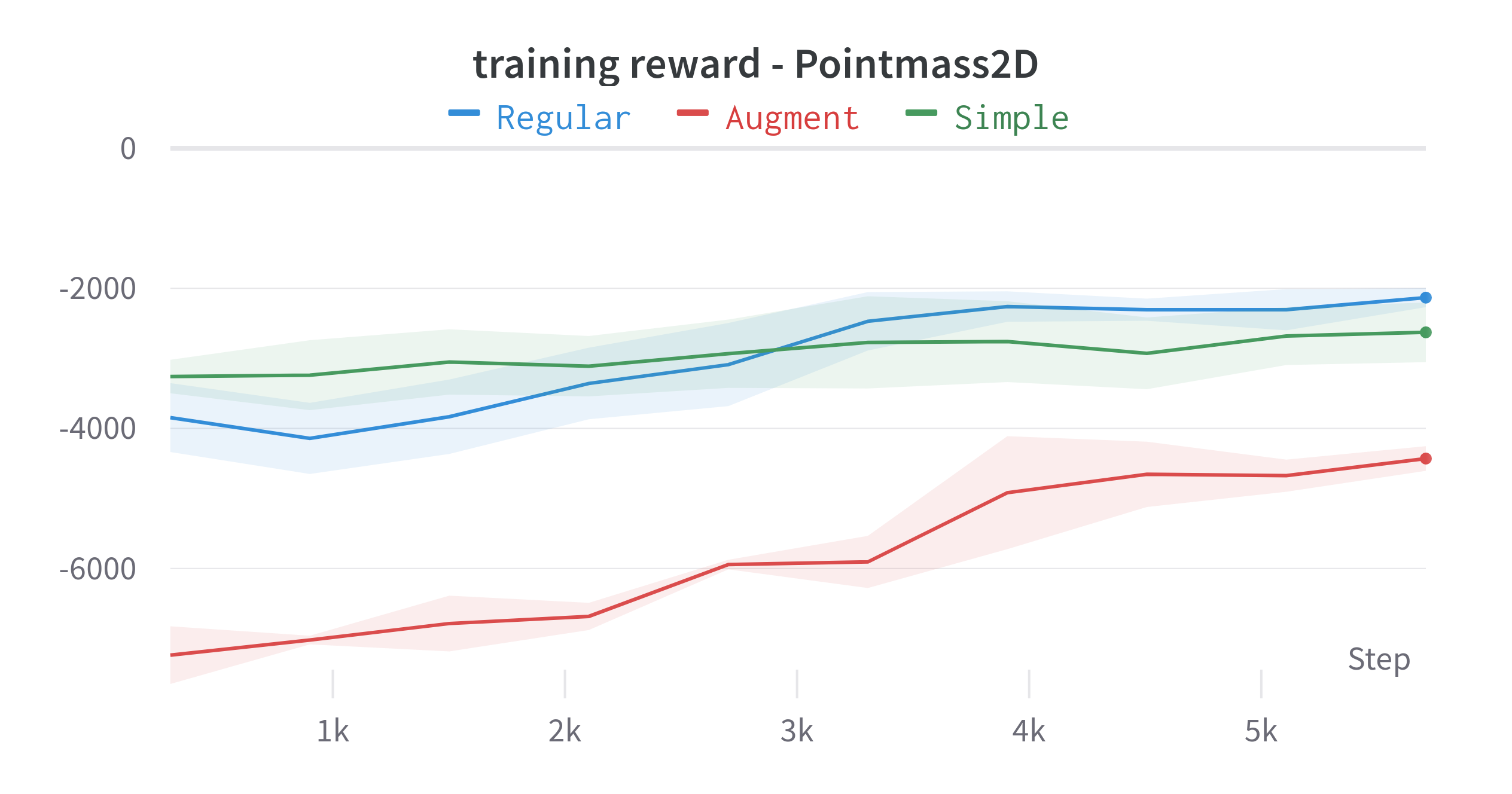
(a) The SF-GPI agent with different feature sets. The higher slope of the learning curve implies a faster learning speed.

(b) When the evaluation task is different from the training one, the baseline SAC[16] fails to generalize to the new task while multi-task agents are less affected.

(c) The hyper-parameter tuning is conducted with the composite task $w^{navigation}=(\mathbf{1},0.5,1)$ and $w^{hover}=(\mathbf{1},1,1)$ and during evaluation, the success weight is increased to 100 for observing the transfer ability. Here we show the best five sets of hyper-parameters.

(d) We compare composition agents with the baseline in the single task $w=(\mathbf{1},0.5,1)$. Baselines SAC[16] is the SOTA maximum entropy RL agent while SQL[14] applies an energy-based training method to achieve expressive multi-modal policy.

Figure 4: Every curve is represented by the mean with two standard deviations of 5 experiments run by the best agent from the hyper-parameter tuning. The hyper-parameter search is conducted by bayesian optimization. We perform in total a hundred searches for every agent. The ablation study indicates that dropout layer can hurt the performance while the effect of other techniques remain unclear, including layernorm, entropy tuning, importance sampling, activation function, etc. Since DAC-GPI behaves fairly similarly to DAC and MSF performs relatively poorly, we neglect them for some experiments.

V-A Network Architecture

We represent primitives and successor features by two neural networks as displayed in Fig. 2. Since the layers or representations are shared, the knowledge transfer can happen within the network. To reduce over-estimation in the SFs and enable higher update-to-data ratio (UTD ratio) [25], we include dropout and layernorm to the SF network. Since ReLU activation can result in negative transfer [22], we incorporate SeLU[26] instead. To further mitigate the positive bias [27], we apply the minimum double critic technique for the SF estimation, i.e., $\hat{\psi}^{\pi}=min(\psi_{\theta_{1}}^{\pi},\psi_{\theta_{2}}^{\pi})$.

V-B Environment and Tasks

We build our training environment in the Raisim[28] simulator, which allows massive vectorization for the environment to collect samples in parallel. Even though Raisim has several built-in robots, to address our problem, we introduce an abstract omnidirectional robot, Pointmass.

V-B1 Pointmass

We first introduce the state and action space of the environment,

• state space $\mathcal{S}$: $\Delta{\mathbb{X}},\Delta{\mathbb{V}},\Delta{\Theta},\Delta{\Omega}\in\mathbb{R}^{3}$, are relative position, velocity, orientation, and angular velocity between the robot and goal respectively.

• action space $\mathcal{A}$: $(a_{x},a_{y},a_{z})$, are the applied force on x-, y-, and z-axis of the Pointmass respectively.

Features, or sub-tasks, can be defined arbitrarily as long as they can be derived from the state space. We pre-define three sets of features for our experiments, as shown in Table. 1. The default will be Regular if not explicitly mentioned.

Regular	$(-|\Delta{\mathbb{X}}|,-||\Delta{\mathbb{V}}||_{2},Success)$
Simple	$(-|\Delta{\mathbb{X}}|)$
Augment	$(-|\Delta{\mathbb{X}}|,-||\Delta{\mathbb{X}}||_{2},-|\Delta{\mathbb{V}}|,-||\Delta{\mathbb{V}}||_{2},Success)$

TABLE 1: Feature sets for Pointmass environment. $|\cdot|$ is the absolute value whereas $||\cdot||_{2}$ is the L2 norm. $Success$ is a binary feature triggered when relative distance is less than 1 meter, i.e., $Success=1$ if $||\mathbb{X}||_{2}<1$ else $0$.

The Regular feature set represents a standard way to define reward functions in robotics, Simple is simplified for the demonstration purpose, and Augment includes the redundant features, and each generates an extra redundant primitive, e.g., both $-|\Delta{\mathbb{X}}|$ and $-||\Delta{\mathbb{X}}||_{2}$ can achieve position control. The goal of each primitive is to maximize its corresponding feature or sub-task. The effect of features is displayed in Fig. 4(a). By adding more features, we obtain more primitives with diverse behavior and increase the learning speed (the slope of the curve).

Though the overall environment is defined in 3D space, it can be reduced to a lower dimension by reducing the action space, e.g., Pointmass2D has the action space $\mathcal{A}=(a_{x},a_{y})$, and in this case, the primitive associated with altitude feature is redundant.

V-B2 Composite Task

We introduce a composite task, which includes two tasks during training, navigation and hover task. The navigation task aims to bring the point mass closer to the goal position, while the hover task requires the robot’s velocity to approach zero when near the goal. The task switches from navigation to hover when the distance to the goal is less than five meters. We can formulate this accordingly,

$$\begin{array}[]{l}w=\begin{cases}w^{navigation}&\text{if $d(s_{pointmass},s_{target})\geq 5m$ }\\ w^{hover}&\text{otherwise}\end{cases}\par\end{array}$$ (36)

where $w^{navigation}=(\mathbf{1},0.5,1)$ and $w^{hover}=(\mathbf{1},20,1)$ and bold symbols denote the vector of the same length as the corresponding feature. Because the velocity penalty is significant when the agent is within the hovering range, the agent will stop immediately for both multi-tasking and standard agents. Now, to test the agents’ transfer capability, in evaluation, we change the composite task to emphasize the success reward, i.e., $w^{navigation}_{eval}=(\mathbf{1},0.5,10000)$ and $w^{hover}_{eval}=(\mathbf{1},20,10000)$. We can demonstrate in Fig. 4(b) that the multi-task agent is less affected when the evaluation task changes.

V-C Training Stability and Composition Noise

The composition noise stems from the action components redundant to the transfer task and it could undermine the training stability. In Pointmass2D-Simple, the primitives corresponding to the features,$-|\Delta{X}|,-|\Delta{Y}|$ produce the distributions $\pi_{x}(a|s)=(\mathcal{N}^{\pi_{x}}_{x},\epsilon)$ and $\pi_{y}=(\epsilon,\mathcal{N}^{\pi_{y}}_{y})$, where $\epsilon$ is the composition noise of unknown distribution (Fig. 3(a)). With MSF, the composite contains the noise in both action components, $\pi^{MSF}=(\mathcal{N}^{\pi_{x}}_{x}\epsilon,\mathcal{N}^{\pi_{y}}_{y}\epsilon)$, whereas SF-GPI contains noise in one of the action components $\pi^{GPI}=(\mathcal{N}^{\pi_{x}}_{x}\epsilon,\mathcal{N}^{\pi_{y}}_{y})$ or $(\mathcal{N}^{\pi_{x}}_{x},\mathcal{N}^{\pi_{y}}_{y}\epsilon)$. Unlike MSF, GPI can utilize critics to select the less noisy one.

Ultimately, only DAC and DAC-GPI can attenuate the noise in both action components, $\pi^{DAC}=((\mathcal{N}^{\pi_{x}}_{x})^{\kappa^{\pi_{x}}_{x}}(\epsilon)^{\kappa^{\pi_{y}}_{x}},(\mathcal{N}^{\pi_{y}}_{y})^{\kappa^{\pi_{x}}_{y}}(\epsilon)^{\kappa^{\pi_{y}}_{y}})$, when the critics reduce $\kappa$ of the noisy term (Fig. 3(b) displays $\kappa$). Fig. 4(c) reflects that the ability to filter out the composition noise is critical to learning speed. DAC-GPI has the best convergence speed, followed by DAC and then SF-GPI. We found the MSF composition unstable due to the composition noise.

Lastly, compared to the maximum entropy RL baselines, i.e., SAC, SQL, in the single task setting (Fig. 4(d)), the multi-task agents show a similar convergence property as SAC.

VI Conclusions and Future Work

Our work unifies the SF-GPI and value composition to the continuous concurrent composition framework and allows reconstructing task policy from a set of primitives. The proposed method was extended to composition at the action component level. We demonstrate in the Pointmass environment that our multi-task agents can reconstruct the task policy from a set of primitives in real time and transfer the skills to solve unseen tasks while the single-task performance is competitive with SAC. This flexible framework incorporates well with the reward-shaping techniques, such as entropy regularization, curiosity[29], etc. In addition, the task-agnostic property should benefit the autotelic framework [30] where agents can set goals and curriculum for themselves [31].

However, the primary concern at this stage is whether the proposed approach can scale to higher dimensional problems. Additionally, two important topics are left as future works. First, look for the corresponding value composition for DAC. A good starting point might be thinking of the MSF composition with weights evaluated by GPE. Second, the optimality of each composition method. One might start with bounding the loss incurred by the policy and value composition.

References

- [1] J. Kober, J. A. Bagnell, and J. Peters, “Reinforcement learning in robotics: A survey,” The International Journal of Robotics Research, vol. 32, no. 11, pp. 1238–1274, 2013.
- [2] M. E. Taylor and P. Stone, “Transfer learning for reinforcement learning domains: A survey.” Journal of Machine Learning Research, vol. 10, no. 7, 2009.
- [3] T. Haarnoja, S. Ha, A. Zhou, J. Tan, G. Tucker, and S. Levine, “Learning to walk via deep reinforcement learning,” Robotics: Science and Systems, 2019.
- [4] A. Barreto, S. Hou, D. Borsa, D. Silver, and D. Precup, “Fast reinforcement learning with generalized policy updates,” Proceedings of the National Academy of Sciences, vol. 117, no. 48, pp. 30 079–30 087, 2020.
- [5] A. Barreto, D. Borsa, S. Hou, G. Comanici, E. Aygün, P. Hamel, D. Toyama, S. Mourad, D. Silver, D. Precup et al., “The option keyboard: Combining skills in reinforcement learning,” Advances in Neural Information Processing Systems, vol. 32, 2019.
- [6] T. Haarnoja, V. Pong, A. Zhou, M. Dalal, P. Abbeel, and S. Levine, “Composable deep reinforcement learning for robotic manipulation,” in 2018 IEEE international conference on robotics and automation (ICRA). IEEE, 2018, pp. 6244–6251.
- [7] J. Hunt, A. Barreto, T. Lillicrap, and N. Heess, “Composing entropic policies using divergence correction,” in International Conference on Machine Learning. PMLR, 2019, pp. 2911–2920.
- [8] B. Van Niekerk, S. James, A. Earle, and B. Rosman, “Composing value functions in reinforcement learning,” in International conference on machine learning. PMLR, 2019, pp. 6401–6409.
- [9] G. Nangue Tasse, S. James, and B. Rosman, “A boolean task algebra for reinforcement learning,” Advances in Neural Information Processing Systems, vol. 33, pp. 9497–9507, 2020.
- [10] R. S. Sutton, D. Precup, and S. Singh, “Between mdps and semi-mdps: A framework for temporal abstraction in reinforcement learning,” Artificial intelligence, vol. 112, no. 1-2, pp. 181–211, 1999.
- [11] X. B. Peng, M. Chang, G. Zhang, P. Abbeel, and S. Levine, “Mcp: Learning composable hierarchical control with multiplicative compositional policies,” Advances in Neural Information Processing Systems, vol. 32, 2019.
- [12] B. D. Ziebart, Modeling purposeful adaptive behavior with the principle of maximum causal entropy. Carnegie Mellon University, 2010.
- [13] R. Fox, A. Pakman, and N. Tishby, “Taming the noise in reinforcement learning via soft updates,” Conference on Uncertainty in Artificial Intelligence. AUAI Press, 2015.
- [14] T. Haarnoja, H. Tang, P. Abbeel, and S. Levine, “Reinforcement learning with deep energy-based policies,” in International conference on machine learning. PMLR, 2017, pp. 1352–1361.
- [15] P. Dayan, “Improving generalization for temporal difference learning: The successor representation,” Neural computation, vol. 5, no. 4, pp. 613–624, 1993.
- [16] T. Haarnoja, A. Zhou, P. Abbeel, and S. Levine, “Soft actor-critic: Off-policy maximum entropy deep reinforcement learning with a stochastic actor,” in International conference on machine learning. PMLR, 2018, pp. 1861–1870.
- [17] P. Pauli, A. Koch, J. Berberich, P. Kohler, and F. Allgöwer, “Training robust neural networks using lipschitz bounds,” IEEE Control Systems Letters, vol. 6, pp. 121–126, 2021.
- [18] R. Munos, T. Stepleton, A. Harutyunyan, and M. Bellemare, “Safe and efficient off-policy reinforcement learning,” Advances in neural information processing systems, vol. 29, 2016.
- [19] S. Schmitt, J. J. Hudson, A. Zidek, S. Osindero, C. Doersch, W. M. Czarnecki, J. Z. Leibo, H. Kuttler, A. Zisserman, K. Simonyan et al., “Kickstarting deep reinforcement learning,” arXiv preprint arXiv:1803.03835, 2018.
- [20] T. Hester, M. Vecerik, O. Pietquin, M. Lanctot, T. Schaul, B. Piot, D. Horgan, J. Quan, A. Sendonaris, I. Osband et al., “Deep q-learning from demonstrations,” in Proceedings of the AAAI Conference on Artificial Intelligence, vol. 32, no. 1, 2018.
- [21] M. Jaderberg, V. Mnih, W. M. Czarnecki, T. Schaul, J. Z. Leibo, D. Silver, and K. Kavukcuoglu, “Reinforcement learning with unsupervised auxiliary tasks,” arXiv preprint arXiv:1611.05397, 2016.
- [22] H. Wang, E. Miahi, M. White, M. C. Machado, Z. Abbas, R. Kumaraswamy, V. Liu, and A. White, “Investigating the properties of neural network representations in reinforcement learning,” arXiv preprint arXiv:2203.15955, 2022.
- [23] A. Paszke, S. Gross, F. Massa, A. Lerer, J. Bradbury, G. Chanan, T. Killeen, Z. Lin, N. Gimelshein, L. Antiga et al., “Pytorch: An imperative style, high-performance deep learning library,” Advances in neural information processing systems, vol. 32, 2019.
- [24] L. Biewald, “Experiment tracking with weights and biases,” 2020, software available from wandb.com.
- [25] T. Hiraoka, T. Imagawa, T. Hashimoto, T. Onishi, and Y. Tsuruoka, “Dropout q-functions for doubly efficient reinforcement learning,” International Conference on Learning Representations (ICLR), 2022.
- [26] G. Klambauer, T. Unterthiner, A. Mayr, and S. Hochreiter, “Self-normalizing neural networks,” Advances in neural information processing systems, vol. 30, 2017.
- [27] S. Fujimoto, H. Hoof, and D. Meger, “Addressing function approximation error in actor-critic methods,” in International conference on machine learning. PMLR, 2018, pp. 1587–1596.
- [28] J. Hwangbo, J. Lee, and M. Hutter, “Per-contact iteration method for solving contact dynamics,” IEEE Robotics and Automation Letters, vol. 3, no. 2, pp. 895–902, 2018. [Online]. Available: www.raisim.com
- [29] D. Pathak, P. Agrawal, A. A. Efros, and T. Darrell, “Curiosity-driven exploration by self-supervised prediction,” in Proceedings of the 34th International Conference on Machine Learning, ser. Proceedings of Machine Learning Research, D. Precup and Y. W. Teh, Eds., vol. 70. PMLR, 06–11 Aug 2017, pp. 2778–2787.
- [30] C. Colas, T. Karch, O. Sigaud, and P.-Y. Oudeyer, “Autotelic agents with intrinsically motivated goal-conditioned reinforcement learning: a short survey,” Journal of Artificial Intelligence Research, vol. 74, pp. 1159–1199, 2022.
- [31] S. Narvekar, B. Peng, M. Leonetti, J. Sinapov, M. E. Taylor, and P. Stone, “Curriculum learning for reinforcement learning domains: A framework and survey,” The Journal of Machine Learning Research, vol. 21, no. 1, pp. 7382–7431, 2020.