Expansion properties of Whitehead moves
on cubic graphs

Abstract.

The present note studies the “graph of graphs” that has cubic graphs as vertices connected by edges represented by the so–called Whitehead moves. We study its conductance and expansion properties, and the adjacency spectrum.

1. Introduction

The present note is concerned with the graph of $3$–regular, or cubic, graphs, and associated objects, such as triangulations and pants decompositions of surfaces. Such a “graph of graphs” $\Gamma_{n}$, represents what can be informally described as the “deformations space” of cubic graphs on $2n$ vertices under the Whitehead moves. In particular, we shall investigate its expansion property.

Expansion is an important notion for families of graphs: we wish to find explicit families of graphs with good expansion properties. In particular, one of the interests of studying expansion is because random walks converge “quickly” to the stationary distribution and how quickly they do is controlled by the second largest eigenvalue of the transition matrix. This notion of rapid mixing turns out to be a very useful measure of expansion for many purposes.

We introduce the notion of outer conductance because there is no standard definition of expansion for directed non–regular multigraphs, despite them being a natural class of objects to consider.

Outer conductance captures how easy it is to escape a given subset of the graph. Therefore, having the outer conductance tend to 0 is a way of saying that the graphs have poor mixing and therefore cannot be “expanders” in this sense.

Let $g$ be a cubic graph (we allow graphs with multiple edges and loops), with set of vertices $V(g)$, and set of edges $E(g)$. Then, for an edge $e\in E(g)$ which is not a loop, there are two possible Whitehead moves $w^{(1)}_{e}$ and $w^{(2)}_{e}$ on $e$, depicted in Figure 1, which are local transformations of $g$. If $e\in E(g)$ is a loop, we assume that the respective Whitehead moves have no effect on $g$.

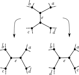
Figure 1. Two possible Whitehead moves performed on an edge $\varepsilon$.

Let the vertices of $\Gamma_{n}$ be all possible cubic graphs on $2n$ vertices ($n\geq 1$) up to isomorphism, where two vertices $g_{1},g_{2}\in V(\Gamma)$ are connected by a directed edge for each Whitehead move $w_{\varepsilon}$, for $\varepsilon\in E(g_{1})$, such that $w_{\varepsilon}(g_{1})$ is isomorphic to $g_{2}$. It is easy to see that being related by a Whitehead move is an equivalence relation on the set of isomorphism classes of cubic graphs on $2n$ vertices ($n\geq 1$).

Such a graph of graphs is related to moduli spaces of surface triangulations [DP19, DP18] and pants decomposition of surfaces [RT13], although not entirely equivalent to said objects. The definition considered here is a directed version of the graph of graphs considered in [RT13]. Since Whitehead moves are reversible, our graph of graphs is quasi–isometric to the one considered in [RT13]. The graph of graphs considered in [RT13] is quasi–isometric to the “wide” component of the thick part of the moduli space of a genus $g\geq 2$ surface. This means that $\Gamma_{n}$ describes pants decompositions of the genus $g=n+1$ surface in which the set of separating curves contains only sufficiently short geodesics. And so is the directed version considered here. Similar local transformations are considered in [Hat99] and two such pants decompositions represent adjacent vertices in $\Gamma_{n}$ if they are connected by an $A$–move, as described in [Hat99], while an $S$–move (also following [Hat99]) is always performed on a handle that corresponds to a loop in the pants decomposition graph, and thus is not taken into account when passing to $\Gamma_{n}$.

Thus, knowing the combinatorial properties of $\Gamma_{n}$ could be useful in the study of the geometric and combinatorial properties of the former.

Here, we introduce a variation $\phi_{out}$ of the usual notion of conductance and show that this quantity tends to $0$ for the family $\Gamma_{n}$ of cubic graphs on $2n$ vertices.

In the present note, we show that the following statements hold.

Theorem A (Theorem 2.2).

Let $\Gamma_{n}$ be the graph of cubic graphs on $2n$ ($n\geq 1$) vertices connected by Whitehead moves. Then $\phi_{out}(\Gamma_{n})\rightarrow 0$, as $n\to\infty$.

Theorem B (Theorem 4.1).

Let $\Gamma_{n}$ be the graph of cubic graphs on $2n$ ($n\geq 1$) vertices. Then the number of length $\ell$ paths in $\Gamma_{n}$ is asymptotically $\sim\rho^{\ell}_{n}$, with $\rho_{n}$ a Perron number.

We also describe how Whitehead moves interact with graph automorphisms in Section 5.

Finally, in Section 6 and LABEL:wm-section:open-questions, we mention some connections and open questions related to $\Gamma_{n}$.

2. Conductance and expansion

Let $G$ be a connected directed graph with vertex set $V(G)$ and edge set $E(G)$. For a subset $S\subset V(G)$, let $d(S)$ denote the sum of vertex out–degrees in $S$, i.e. $d(S)=\sum_{v\in S}deg_{out}(v)$, where $d_{out}(v)$ is the number of edge of the form $(v,u)$ where $v,u\in V(G)$. The boundary $\partial(S)$ of a vertex subset $S\subset V(G)$ is defined as the number of directed edges in $E(G)$ joining a vertex in $S$ with a vertex in $V(G)\setminus S$, that is $\partial(S)=\{e=(u,v)\in E(G)\ |\ u\in S\ ,v\in S^{c}\}$.

The outer–conductance of $S\subset V(G)$ is defined as follows:

$$\phi_{out}(S)=\frac{|\partial(S)|}{\min\{d(S),d(V(G)-S)\}}$$

and the outer–conductance of $G$ is

$$\phi_{out}(G)=\min_{S\subset V(G)}\phi_{out}(S).$$

This is a generalization of the notion of conductance [CG97]. Since we work with directed graphs, the definition is adapted so that the volume is measured with respect to the number of out–going edges. By doing so the outer–conductance measures how hard it is to escape a subset of the graph.

As a generalisation of the notion of expander families to the case of directed graphs with vertex degrees (both out–degree and in–degree) growing with the number of vertices, we introduce Definition 2.1.

Definition 2.1.

We say that a sequence of directed graphs $G_{n}$ with out–degree and in–degree growing with the number of vertices is an outer–expander family if the conductance $\phi_{out}(G_{n})$ is uniformly bounded away from 0 as $n$ tends to infinity.

Now we prove our first assertion.

Theorem 2.2.

Let $\Gamma_{n}$ be the directed graph of cubic graphs on $2n$ ($n\geq 1$) vertices connected by Whitehead moves. Then $\Gamma_{n}$ is connected and $\phi_{out}(\Gamma_{n})\rightarrow 0$, as $n\to\infty$. Therefore, the family $\{\Gamma_{n}\}_{n\in\mathbb{N}}$ is not a family of outer–expanders.

3. Proof of Theorem 2.2

Let $\Gamma_{n}$ be the directed graph of (isomorphism classes of) cubic graphs on $2n$ vertices ($n\geq 1$). The following two claims will imply Theorem 2.2.

$\Gamma_{n}$ is connected.

This follows from [RT13]. Even simpler, by means of Whitehead moves we can bring every cubic graph to a certain uniquely determined cubic tree.

Figure 2. Performing a Whitehead move on the edge $\varepsilon=(v_{0},v_{1})$ that belongs to a $k$–cycle $C_{k}$ in $g\in V(\Gamma_{n})$.

Let $g$ be a cubic graph, and let $C_{k}$ be an indecomposable $k$–cycle (with $k\geq 2$) in $g$, i.e. an induced cycle subgraph where no edge of $g$ connects any two vertices of $C_{k}$, except the edges of $C_{k}$ itself. If we perform a Whitehead move on the edge $\varepsilon$ that belongs to a $k$–cycle $C_{k}$, a part of which is depicted in Figure 2, we obtain a modified graph (partly) depicted in Figure 3.

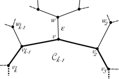
Figure 3. A $(k-1)$–cycle $C_{k-1}$ in $\tilde{g}=w_{\varepsilon}(g)$: the edge $\varepsilon=(v,w)$ does not belong to $C_{k-1}$.

The overall changes in the structure of $\tilde{g}=w_{\varepsilon}(g)$ as compared to $g$ are local and amount to the following:

• The $k$–cycle $C_{k}$ has been transformed into a $(k-1)$–cycle $C_{k-1}$ ;

• If $v_{1}$, $w_{1}$ were part of an $l$–cycle $C_{l}$ then $C_{l}$ was transformed into an $(l+1)$–cycle $C_{l+1}$;

• Same applies to any cycle that previously contained $w_{0}$ and/or $v_{0}$.

By performing a total of $k-1$ Whitehead moves on the edges in $C_{k}$, we reduce it to a loop, as depicted in Figure 4. Here we reduced the total amount of $k$–cycles with $k\geq 2$ by one, although the lengths of some other cycles could have been augmented.

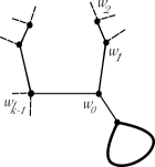
Figure 4. A $k$–cycle $C_{k}$ ($k\geq 2$) is reduced to a loop by $k-1$ consecutive Whitehead moves.

By repeating the above procedure on the remaining $k$–cycles (with $k\geq 2$) of the resulting graph, we shall reduce it to what we call a $(n,b)$–cubic tree, an example of which is depicted in Figure 5. Such a tree has $2n$ vertices and $b=n+1$ loops (note that $b$ is the $1$st Betty number of the initial graph $g$, since Whitehead moves preserve the number of vertices and edges of $g$, as well as the rank of $\pi_{1}(g)$).

Figure 5. A $(2,3)$–cubic tree

There exists a natural isomorphism between our $(n,b)$–cubic trees with a chosen loop (i.e. rooted $(n,b)$–cubic trees with a chosen loop $\varepsilon^{*}$ as a root), and binary rooted trees. Namely, let us take a rooted $(n,b)$–cubic tree $(T,\varepsilon^{*})$ and remove all the loops as well as the edge $(v^{*},v)$ adjacent to $\varepsilon^{*}$ (with $\varepsilon^{*}$ being a loop at vertex $v$). The result, $(\tilde{T},v^{*})$ is a binary rooted tree on $2n-1$ vertices with $n$ leaves.

As shown in  Figure 6, a tree rotation can be achieved by a Whitehead move. Thus, $(\tilde{T},v^{*})$ can be brought to the unique complete rooted binary tree $T_{n}$ on $n$ vertices, cf. [CLRS09, §12 – §13] for more information on binary trees and tree rebalancing. This proves that $\Gamma_{n}$ is connected.

Figure 6. A left and right rotation of a rooted binary tree (corresponding to an $(n,b)$–cubic tree with root $\varepsilon^{*}$) realised by a Whitehead move on edge $e$. Here $P$, $Q$ are the vertices of $\varepsilon$, and $A$, $B$, and $C$ are the respective sub–trees

The outer–conductance of $\Gamma_{n}$ tends to 0.

Let $B_{n}\subset V(\Gamma_{n})$ be the set of (isomorphism classes of) connected cubic graphs on $2n$ vertices that have at least one bridge. We shall estimate the probability $\mathbb{P}(g\in B_{n})$ asymptotically. For this matter, notice that if $U_{n}=V(\Gamma_{n})$ is the set of unlabelled cubic graphs (i.e. their isomorphism classes), and $L_{n}$ is the set of labelled ones, then $\mathbb{P}(g\in U_{n}\mbox{ has a bridge})=\mathbb{P}(g\in L_{n}\mbox{ has a bridge})+o(1)$, since asymptotically virtually all graphs in $L_{n}$ have no non–trivial automorphisms [Bol82], and thus $|L_{n}|\sim|U_{n}|\cdot(2n)!$, as $n\to\infty$.

A bridge in a connected graph is an edge such that its removal produces several connected components. A graph with a bridge is called bridged, while a graph that has no bridges at all is called bridgeless.

A Hamiltonian circuit in a (connected) graph is a closed edge path without self–intersection that visits each vertex once. A graph is called Hamiltonian if it admits a Hamiltonian circuit.

It is clear that a graph that has a bridge cannot be Hamiltonian, and that every Hamiltonian cubic graph is bridgeless.

Let $Bridged=\{g\in L_{n}\ |\ g\mbox{ has a bridge}\}$ and $Looped=\{g\in L_{n}\ |\ g\mbox{ has a loop}\}$, and let $nH$ be the set of graphs in $L_{n}$ that do not have a Hamiltonian circuit. Then

$$\mathbb{P}(g\in Looped)\leq\mathbb{P}(g\in Bridged)\leq\mathbb{P}(g\in Looped)+\mathbb{P}(g\notin Looped\mbox{ \& }g\in nH),$$

since $Looped\subseteq Bridged$, as well as $Bridged\subseteq nH$.

By applying [JLR11, Theorem 9.5], we have that $\mathbb{P}(g\in Looped)=1-e^{-1}+o(1)$, while [JLR11, Theorem 9.23] implies that $\mathbb{P}(g\notin Looped\mbox{ and }g\in nH)=o(1)$, as $n\to\infty$. Thus, $\mathbb{P}(g\in Bridged)=1-e^{-1}+o(1)$ asymptotically, as $n\to\infty$.

Together with the remarks above about the probabilities for labelled and unlabelled graphs, we obtain that $\mathbb{P}(g\in B_{n})$, for $g\in V(\Gamma_{n})$, satisfies $\mathbb{P}(g\in B_{n})=1-e^{-1}+o(1)$, as $n\to\infty$. Thus, $|B_{n}|\sim(1-e^{-1})|V(\Gamma_{n})|$, and $|V(\Gamma_{n})\setminus B_{n}|\sim e^{-1}|V(\Gamma_{n})|$.

Note that the only vertices in $B_{n}$ connected with vertices in $V(\Gamma_{n})\setminus B_{n}$ are those $g\in B_{n}$ having a single bridge, and the corresponding Whitehead moves have to be performed exactly on the bridge edge of $g$.

Indeed, let $g\in V(\Gamma_{n})$ have at least one bridge and let $\varepsilon^{*}=(u,v)$ denote one of its bridges. Then we can check case–by–case what the result of a Whitehead move on $\varepsilon^{*}$ could be.

For this purpose, let us introduce the following equivalence relation on the vertices of $g$: for $v,w\in V(g)$, we write $v\sim_{g}w$ if and only if there are two edge–disjoint paths connecting $v$ to $w$. Then we write $[v]_{g}=\{w\in V(g)\ s.t.\ v\sim_{g}w\}$ for the equivalence class of $v$.

Let $\{a,b,c,d\}$ be the vertices adjacent to the bridge $\varepsilon^{*}\in E(g)$, and let $\tilde{g}=w_{\varepsilon^{*}}(g)$ be the graph resulting from a Whitehead move performed on $\varepsilon^{*}$. Then we consider the following five possible cases.

1.

$[a]_{g}=[b]_{g}=[c]_{g}=[d]_{g}$: in this case $\varepsilon^{*}$ is not a bridge neither in $g$, nor in $\tilde{g}$, cf. Figures 8 and 8.

2.

$[a]_{g}=[b]_{g}=[c]_{g}\neq[d]_{g}$: same as above, $\varepsilon^{*}$ is not a bridge neither in $g$, nor in $\tilde{g}$, cf. Figures 10 and 10.

3.

$[a]_{g}=[b]_{g}\neq[c]_{g}=[d]_{g}$: in this case, $\varepsilon^{*}$ is a bridge in $g$, but not in $\tilde{g}$, cf. Figures 12 and 12.

4.

$[a]_{g}=[b]_{g}\neq[c]_{g}$ , $[a]_{g}=[b]_{g}\neq[d]_{g}$, and $[c]_{g}\neq[d]_{g}$: again, $\varepsilon^{*}$ is a bridge in $g$, but not in $\tilde{g}$, cf. Figures 14 and 14.

5.

$[a]_{g},[b]_{g},[c]_{g},[d]_{g}$ are all distinct: obviously, $\varepsilon^{*}$ is a bridge in both $g$ and $\tilde{g}$, cf. Figures 16 and 16.

Figure 7. Local picture inside $g$ when $[a]_{g}=[b]_{g}=[c]_{g}=[d]_{g}$

Figure 8. Local picture inside $\tilde{g}$ when $[a]_{g}=[b]_{g}=[c]_{g}=[d]_{g}$

Figure 9. Local picture inside $g$ when $[a]_{g}=[b]_{g}=[c]_{g}\neq[d]_{g}$

Figure 10. Local picture inside $\tilde{g}$ when $[a]_{g}=[b]_{g}=[c]_{g}\neq[d]_{g}$

Figure 11. Local picture inside g when $[a]_{g}=[b]_{g}\neq[c]_{g}=[d]_{g}$

Figure 12. Local picture inside $\tilde{g}$ when $[a]_{g}=[b]_{g}\neq[c]_{g}=[d]_{g}$

Figure 13. Local picture inside $g$ when $[a]_{g}=[b]_{g}\neq[c]_{g}$ , $[a]_{g}=[b]_{g}\neq[d]_{g}$, and $[c]_{g}\neq[d]_{g}$

Figure 14. Local picture inside $\tilde{g}$ when $[a]_{g}=[b]_{g}\neq[c]_{g}$ , $[a]_{g}=[b]_{g}\neq[d]_{g}$, and $[c]_{g}\neq[d]_{g}$

Figure 15. Local picture inside $g$ when $[a]_{g},[b]_{g},[c]_{g},[d]_{g}$ are all distinct

Figure 16. Local picture inside $\tilde{g}$ when $[a]_{g},[b]_{g},[c]_{g},[d]_{g}$ are all distinct

According to the observations above, if a bridged graph $g\in B_{n}$ can be transformed into a bridgeless one $\tilde{g}=w_{\varepsilon}(g)$, then $\varepsilon$ is the only bridge of $g$. Every time, both Whitehead moves either succeed or fail to bring $\tilde{g}$ outside $B_{n}$. This implies that $|\partial(B_{n})|\leq 2|B_{n}|$. Thus the outer–conductance of the set $B_{n}$ satisfies

$$\phi_{out}(B_{n}) =\frac{|\partial(B_{n})|}{\min\{d(B_{n}),d(V(\Gamma_{n})\setminus B_{n})\}}\leq\frac{2|B_{n}|}{6n|V(\Gamma_{n})\setminus B_{n}|}\sim$$

$$\sim\frac{2|V(\Gamma_{n})|(1-e^{-1})}{6n|V(\Gamma_{n})|e^{-1}}=\frac{e-1}{3n}\to 0,$$

as $n\to\infty$. $\square$

4. Adjacency spectrum

Let $A$ be a non–zero square $k\times k$ ($k\geq 2$) matrix with non–negative integer entries. Such a matrix is called non–negative, for brevity. If all the entries of $A$ are actually positive, then $A$ is called positive.

If there exists a permutation matrix $P$ such that $PAP^{-1}$ has upper–triangular block form, $A$ is called reducible. Otherwise, $A$ is irreducible.

For $i\in\{1,\dots,k\}$, the $i$–th period of $A$ is the least positive integer $m$ such that the $i$–th diagonal entry of $A^{m}$ is positive. If $A$ is irreducible, then all its periods coincide, and each of them equals the period of $A$. If the period of $A$ equals $1$, then $A$ is called aperiodic.

An aperiodic and irreducible non–negative matrix $A$ is called primitive. If $A$ is a primitive matrix, then its spectral radius is a Perron number, as a consequence of the Perron–Frobenius theorem [LM21]. Recall that a Perron number is an algebraic integer $\rho>1$ such that all of its other Galois conjugates have modulus strictly less than $\rho$. Perron numbers often appear in dynamical context, cf. [LM21]. Another property of the spectral radius of a primitive matrix $A$ is that this eigenvalue has multiplicity one.

Let $\Gamma$ be a directed graph, and let $A$ be its adjacency matrix defined as follows:

$$A_{uv}=\mbox{ the number of directed edges joining }u\mbox{ to }v,\mbox{ if }u\neq v,\mbox{ and }$$

$$A_{vv}=\mbox{ the number of loops incident to }v.$$

Then $A$ is irreducible if and only if $\Gamma$ is strongly connected, i.e. there exists a path of directed edges in $\Gamma$ between any pair of distinct vertices. If $\Gamma$ is strongly connected and the greatest common divisor of its directed cycles equals $1$, then $A$ is aperiodic, and thus primitive. Thus, in this case we can deduce that the spectral radius of $A$ is a Perron number by considering the combinatorics of $\Gamma$.

Theorem 4.1.

Let $\Gamma_{n}$ be the graph of cubic graphs on $2n$ ($n\geq 1$) vertices. Then the number of length $\ell$ paths in $\Gamma_{n}$ is asymptotically $\sim\rho^{\ell}_{n}$, with $\rho_{n}$ a Perron number.

4.1. Proof of Theorem 4.1

Let $\Gamma_{n}$ be the graph of graphs on $2n$ vertices ($n\geq 1$), and let $A_{n}=A(\Gamma_{n})$ be its adjacency matrix. We want to show that $A_{n}$ is primitive. This would imply that its spectral radius $\rho_{n}=\rho(A_{n})$ is a multiplicity $1$ eigenvalue with a positive eigenvector $v$, and that $\rho_{n}$ is a Perron number. The asymptotic number of paths is then a standard computation.

For every $n\geq 1$, there exists an $(n,b)$–cubic tree $t\in V(\Gamma_{n})$, with $b=n+1\geq 2$ loops $\varepsilon_{1},\dots,\varepsilon_{b}$. Then, $w_{\varepsilon_{i}}(t)=t$, for any $i=1,\dots,b$, and thus $\Gamma_{n}$ has loops. This implies that $\Gamma_{n}$ is aperiodic.

We already know that that $\Gamma_{n}$ is strongly connected, as in Theorem 2.2 we prove that $\Gamma_{n}$ is connected as a directed graph. Thus, we obtain that $A_{n}$ is also primitive, and can now apply the Perron–Frobenius theorem. $\square$

4.2. Remark on the thin neighbourhood.

It appears that $\Gamma_{n}$ is itself a relatively “thin” neighbourhood of $B_{n}$. Indeed, we each length $k$ cycle in a graph $g\in V(\Gamma_{n})$ can be reduced by $k-2$ Whitehead moves to a $2$–cycle, and one more Whitehead move will create an edge incident to a loop. The standard asymptotic bound on girth is $\mathrm{girth}(g)\lesssim 2\log_{2}n$. If $v=|V(\Gamma_{n})|$, then $v\sim n^{n}$ [Bol82], and thus each vertex of $\Gamma_{n}$ happens to be within $\sim\log_{2}\log_{2}v$ distance from $B_{n}$. As shown in [RT13], the diameter of $\Gamma_{n}$ satisfies $d=\mathrm{diam}(\Gamma_{n})\sim n\log_{2}n$, and thus each vetrex of $\Gamma_{n}$ is within $\log_{2}d$ of $B_{n}$.

5. Edge orbits and automorphisms

Below we make some remarks on how performing Whitehead moves on edges equivalent under graph automorphisms affects the resulting graph.

Proposition 5.1.

Let $g$ be a trivalent graph and $e,f\in E(g)$. Suppose there exists an automorphism $\alpha\in Aut(g)$ of $g$ such that $\alpha(e)=f,\alpha(v_{i})=w_{i}$ and $\alpha(e_{i})=f_{i}$ for the corresponding indices and that all the $v_{i}$’s and $w_{i}$’s are distinct (see 18 and 18).

Then, if we perform the same Whitehead move on both sides, that is we choose one of the following pairs of transformations:

1. $w_{e}^{1}:(v_{1},v_{2})(v_{3},v_{4})\mapsto(v_{1},v_{3})(v_{2},v_{4})$ and $w_{f}^{1}(g):(w_{1},w_{2})(w_{3},w_{4})\mapsto(w_{1},w_{3})(w_{2},w_{4})$; or

2. $w_{e}^{2}:(v_{1},v_{2})(v_{3},v_{4})\mapsto(v_{1},v_{4})(v_{2},v_{3})$ and $w_{f}^{2}:(w_{1},w_{2})(w_{3},w_{4})\mapsto(w_{1},w_{4})(w_{2},w_{3})$,

then the resulting graphs are isomorphic $w_{e}^{1}(g)\cong w_{f}^{1}(g)$ and $w_{e}^{2}(g)\cong w_{f}^{2}(g)$.

Figure 17. The neighbourhood of $e$

Figure 18. The neighbourhood of $f$

Proof.

Suppose we perform a Whitehead move of type (1). Consider $g_{1}=g\setminus St(e)$ and $g_{2}=\alpha(g)\setminus St(f)$ where $St(e)$, resp. $St(f)$, is the star of $f$, resp. $e$ (i.e. the set of incident vertices and edges to $e$, resp. $f$).

Then the map $\alpha$ induces $\overline{\alpha}:g_{1}\to g_{2}$ which is an isomorphism.

Now consider $\gamma_{1}=w_{e}^{1}(g)\setminus St(e)$ and $\gamma_{2}=w_{f}^{1}(g)\setminus St(f)$. Since a Whitehead move is a local transformation, we have that $g_{1}=\gamma_{1}$ and $g_{2}=\gamma_{2}$. Thus, we obtain a map $\overline{\alpha}:\gamma_{1}\to\gamma_{2}$, and this map is a graph isomorphism.

Now we can extend $\overline{\alpha}$ to a map from $\gamma_{1}=w_{e}^{1}(g)$ to $\gamma_{2}=w_{f}^{1}(g)$ in the unique possible way, because $v_{1}$ and $v_{3}$ have a unique common neighbour in $St_{w_{e}^{1}(g)}(e)$ and the same applies to $w_{1},w_{3}$ in $St_{w_{f}^{1}(g)}(f)$. The same can be done for $v_{2},v_{4}$ and $w_{2},w_{4}$. Thus, the map obtained is a graph isomorphism between $\gamma_{1}$ and $\gamma_{2}$.

Note that exactly the same proof applies if we perform a Whitehead move of type (2). ∎

Note also that the same proof works if, for example, $v_{1}=v_{3}$ and $w_{1}=w_{3}$ and/or $v_{2}=v_{4}$ and $w_{2}=w_{4}$. The main point being that multiple edges still allow extending the automorphism.

We also have a sort of converse.

Proposition 5.2.

Suppose $w_{e}^{k}(g)\cong w_{f}^{k}(g)$ via a map $\psi$ such that $\psi(e^{*})=f^{*},\psi(v_{i}^{*})=w_{i}^{*}$ and $\psi(e_{i}^{*})=f_{i}^{*}$ for the corresponding indices $i$ (see Figures 20 and 20). Then, there exists $\overline{\psi}\in Aut(g)$ such that $\overline{\psi}(e)=f$.

Figure 19. The neighbourhood of $e^{*}$ in $w_{e}^{k}(g)$

Figure 20. The neighbourhood of $f^{*}$ in $w_{f}^{k}(g)$

Proof.

Starting from the two graphs, re–apply the corresponding Whitehead moves, that is either apply on both sides $w_{e}^{1}$ and $w_{f}^{1}$ or $w_{e}^{2}$ and $w_{f}^{2}$ . The two graphs obtained are isomorphic, and on both sides you retrieve $g$. Now you can apply Proposition 5.1 and thus obtain the desired $\overline{\psi}$. ∎

Proposition 5.3.

Suppose $g_{1}$ and $g_{2}$ are isomorphic trivalent graphs via a map $\phi$. Suppose $g_{1}=w_{e}^{1}(h_{1})$ and $g_{2}=w_{f}^{1}(h_{2})$. Suppose that the map $\phi$ maps $e^{*}=w_{e}^{1}(e)$ to $f^{*}=w_{e}^{1}(f)$ and the incident vertices $v_{i}^{*}$ to $w_{i}^{*}$ as in Figures 20 and 20. Then $h_{1}$ and $h_{2}$ are isomorphic and there exists an isomorphism $\psi:h_{1}\to h_{2}$ that maps $e$ onto $f$.

Proof.

Consider $\Gamma_{1}=g_{1}\setminus St(e^{*})$ and $\Gamma_{2}=g_{2}\setminus St(f^{*})$. Then $\phi$ induces $\overline{\phi}:\Gamma_{1}\to\Gamma_{2}$ and $\overline{\phi}$ is an isomorphism of graphs. Note that since a Whitehead move is a local transformation, we have that $\Gamma_{1}=h_{1}\setminus St(e)$ and $\Gamma_{2}=h_{2}\setminus St(f)$ thus $\overline{\phi}$ can be seen as a map from $h_{1}\setminus St(e)$ to $h_{2}\setminus St(f)$. We will now extend $\overline{\phi}$ to an isomorphism $\psi:h_{1}\to h_{2}$.

Suppose the transformation $h_{1}\to g_{1}$ was doing (as local changes described in $h_{1}$) $(v_{1}v_{3})(v_{2}v_{4})\to(v_{1}v_{2})(v_{3})(v_{4})$ and the transformation $h_{2}\to g_{2}$ was doing (as local changes in $h_{2}$) $(w_{1}w_{2})(w_{3}w_{4})\to(w_{1}w_{2})(w_{3}w_{4})$.This is always possible up to relabelling the graphs. Then $\{e_{1}\}=St_{h_{1}}(v_{1})\cap St_{h_{1}}(v_{3}),\{e_{2}\}=St_{h_{1}}(v_{2})\cap St_{h_{1}}(v_{4}),\{f_{1}\}=St_{h_{2}}(w_{1})\cap St_{h_{2}}(w_{3}),\{f_{2}\}=St_{h_{2}}(w_{2})\cap St_{h_{2}}(w_{4})$ and we define $\psi:h_{1}\to h_{2}$ as follows. We set $\psi(e_{i})=f_{i}$ and ${\left.\kern-1.2pt\psi\vphantom{\big{|}}\right|_{h_{1}\setminus St(e)}}=\overline{\phi}$. Obviously $\psi$ is an isomorphism of graphs and it maps $e$ to $f$ because we extend it to preserve adjacency. ∎

6. Related objects

Above we consider the graph of graphs $\Gamma_{n}$ of all possible cubic graphs on $2n$ vertices, where two vertices, $g_{1},g_{2}\in V(\Gamma_{n})$, are connected by a directed edge for each Whitehead move $w_{\varepsilon}$, for $\varepsilon\in E(g_{1})$, such that $w_{\varepsilon}(g_{1})$ is isomorphic to $g_{2}$ vertices up to isomorphism.

However, there are several ways to modify this definition. Indeed, we could modify the edges of $\Gamma_{n}$ in order to turn it into an undirected graph, a simple graph or other types of graphs. These modifications can provide relations between the graph of graphs and other mathematical problems. In this section we will explore some of these connections.

6.0.1. Matchings on graphs

If two edges $e$, $f$ in $g\in\Gamma_{n}$ are not incident to each other, then $w_{e}(g)$ and $w_{f}(g)$ commute. That is, if we want to apply consecutively the two transformations, it will yield the same graph. This comes from Whitehead moves being local transformations of the graph. Thus, if the two local transformations are “far away” from each other, they commute. We will call this a simultaneous Whitehead move on the set $\{e,f\}$ or simultaneous WM for short.

Thus, we can modify slightly the edges of $\Gamma_{n}$ to make it into a simple directed graph in the following way. Say $g_{1},g_{2}\in V(\Gamma_{n})$, are connected by an undirected edge if there exists some Whitehead move on some set of non–incident edges of $g_{1}$ mapping $g_{1}$ to $g_{2}$.

Then, the maximal number of edges one could choose in $g_{1}$ to perform a simultaneous WM is the cardinality of a maximum matching in $g_{1}$. Thus, determining the degree of $\Gamma_{n}$ as defined in this paragraph is closely related to the number of matchings in a trivalent multigraph, though the two quantities are not necessarily equal. Indeed, the number of maximum matchings in $g_{1}$ yields an upper bound on the degree of $g_{1}$ in $\Gamma_{n}$.

6.0.2. Outer space and its spine

In [CV86], Culler and Vogtmann introduced a space $X_{n}$ on which the group $Out(F_{n})$ acts. This space can be thought of as analogous to the Teichmüller space of a surface with the action of the mapping class group of the surface.

The description of $X_{n}$ is complicated, and we will not detail it here. We will only briefly mention the relevant aspects of this object and how it could relate to our graph of graphs.

The space $X_{n}$ is an infinite, finite–dimensional simplicial complex. A point in a simplex in $X_{n}$ can be thought of as a metric graph (we assign lengths to the edges of the graph) with fundamental group $F_{n}$ and some labelling on its edges representing an element $\phi\in Out(F_{n})$ (these are called marked metric graphs). Two given $k$–simplices $x_{1}$ and $x_{2}$ share a face of codimension $1$ if passing from the representative of $x_{1}$ to the one of $x_{2}$ can be obtained by quotienting an edge and re–opening it. Thus, some simplices have open faces : the ones where collapsing an edge would change the fundamental group on the underlying graph (that is, “killing” a generator of $F_{n}$). Note that maximal dimension simplices correspond to marked trivalent metric graphs.

The space $X_{n}$ admits a spine $K_{n}$ which is a deformation retract of $X_{n}$ in which we “forget” about the lengths of the edges. This spine $K_{n}$ has the structure of a simplicial complex, in fact it can be identified with the geometric realization of the partially ordered set of open simplices of $X_{n}$. The group $Out(F_{n})$ acts on $K_{n}$ with compact quotient.

Our graph of graphs $\Gamma_{n}$ is related to $K_{n}/Out(F_{n})$ in the following way. First, we need to slightly modify the graph $\Gamma_{n}$: say $g_{1},g_{2}\in V(\Gamma_{n})$ are connected by a directed edge from $g_{1}$ to $g_{2}$ for each edge $e\in g_{1}$ such that $w_{e}^{1}(g)\cong g_{2}$ or $w_{e}^{2}(g)\cong g_{2}$. That is, we record on which edge we performed the Whitehead move but not the type of Whitehead move.

A vertex $g\in\Gamma_{n}$ has fundamental group isomorphic to $F_{n}$ and thus corresponds to a simplex in $K_{n}/Out(F_{n})$. In particular, since $g$ is a cubic graph, it corresponds to a maximal simplex in $K_{n}/Out(F_{n})$. Thus, two vertices $g_{1}$ and $g_{2}$ are adjacent in $\Gamma_{n}$ if and only if the corresponding simplices in $K_{n}/Out(F_{n})$ share a face of codimension $1$ (a wall).

If we set $w(g_{1},g_{2})=\min\{\#E(g_{1},g_{2}),\#E(g_{2},g_{1})\}$, then the number $w(g_{1},g_{2})$ represents the number of walls shared by the corresponding simplices in $K_{n}/Out(F_{n})$. Moreover, the edges chosen to perform the Whitehead moves on indicate the edges to collapse to describe the shared walls. Thus, our graph of graphs can be thought as encoding adjacency between maximal simplices in $K_{n}/Out(F_{n})$ while keeping track of their shared walls.

References

- [Bol82] Béla Bollobás. The asymptotic number of unlabelled regular graphs. Journal of the London Mathematical Society, 2(2):201–206, 1982.
- [CG97] Fan RK Chung and Fan Chung Graham. Spectral graph theory. American Mathematical Soc., 1997.
- [CLRS09] Thomas H Cormen, Charles E Leiserson, Ronald L Rivest, and Clifford Stein. Introduction to algorithms. MIT press, 2009.
- [CV86] Marc Culler and Karen Vogtmann. Moduli of graphs and automorphisms of free groups. Inventiones mathematicae, 84(1):91–119, 1986.
- [DP18] Valentina Disarlo and Hugo Parlier. Simultaneous flips on triangulated surfaces. Michigan Mathematical Journal, 67(3):451–464, 2018.
- [DP19] Valentina Disarlo and Hugo Parlier. The geometry of flip graphs and mapping class groups. Transactions of the American Mathematical Society, 372(6):3809–3844, 2019.
- [Hat99] Allen Hatcher. Pants decompositions of surfaces. arXiv preprint math/9906084, 1999.
- [JLR11] Svante Janson, Tomasz Luczak, and Andrzej Rucinski. Random graphs, volume 45. John Wiley & Sons, 2011.
- [LM21] Douglas Lind and Brian Marcus. An introduction to symbolic dynamics and coding. Cambridge university press, 2021.
- [RT13] Kasra Rafi and Jing Tao. The diameter of the thick part of moduli space and simultaneous whitehead moves. Duke Mathematical Journal, 162(10):1833–1876, 2013.
- [Vog02] Karen Vogtmann. Automorphisms of free groups and outer space. Geometriae Dedicata, 94:1–31, 2002.