Master Stability Functions of Networks of Izhikevich Neurons

Abstract

Synchronization has attracted the interest of many areas where the systems under study can be described by complex networks. Among such areas is neuroscience, where is hypothesized that synchronization plays a role in many functions and dysfunctions of the brain. We study the linear stability of synchronized states in networks of Izhikevich neurons using Master Stability Functions, and to accomplish that, we exploit the formalism of saltation matrices. Such a tool allows us to calculate the Lyapunov exponents of the Master Stability Function (MSF) properly since the Izhikevich model displays a discontinuity within its spikes. We consider both electrical and chemical couplings, as well as total and partially synchronized states. The MSFs calculations are compared with a measure of the synchronization error for simulated networks. We give special attention to the case of electric and chemical coupling, where a riddled basin of attraction makes the synchronized solution more sensitive to perturbations.

I Introduction

Neurons are the building blocks of the brain. These structures can display a rich variety of dynamics depending on their type and the inputs that it receives from other neurons [1]. Although many features of neurons remain unclear, models are capable of reproducing their observed dynamics. The seminal work of Hodgkin-Huxley (HH) introduced a neuron model based on the giant axon of the squid [2]. Being biophysically accurate, this model become a standard for ODE-based neuron models. Naturally, the collective dynamics of neurons are also of interest, and unfortunately, networks of complex models like the HH can be difficult to deal with both analytically and computationally. With this in mind, E. M. Izhikevich proposed a neuron model that combines biological features of complex models, like the HH, with computational efficiency [3].

Due to these characteristics, the Izhikevich model has been implemented in the study of networks of spiking neurons, including large-scale models [4, 5]. Such models can be used to deepen our understanding of how the interplay between synaptic and neuronal processes produces collective behaviors. Of great interest is the emergence of rhythms and synchronization of neural activity, as it suggests that the high-dimensional dynamics of neuronal networks can collapse into low dimensional oscillatory modes [6]. Although rhythmic activity and synchronization are often associated with brain pathologies like Parkinson’s disease and epilepsy [7, 8], evidence suggests that these two mechanics are involved in information processing, memory formation, and cognition [9, 10, 11].

Since the mathematical description of synchronization is well established in nonlinear dynamics, it can be applied to many natural phenomena, including neural activity. A central question regarding synchronization theory is whether a synchronized state is stable or not. Among the many contributions to this topic over the last decades, here we focus on the Master Stability Function (MSF) formalism [12]. The main result of such formalism is a diagonalized variational equation, which allows us to calculate the Lyapunov exponents associated with perturbations transverse to the synchronized manifold. In the original work, it was made possible by assuming that the system can be locally linearized around the synchronized solution, as well as a diagonalizable coupling matrix. Fortunately, this formalism has been extended to a variety of cases including near-identical systems, non-diagonalizable, and multilayer networks [13, 14, 15]. Moreover, the stability of partial synchronization, which includes cluster synchronized and chimera states have also been studied in the context of master stability functions [16, 17, 18, 19].

In this paper, we apply the MSF formalism to study the linear stability of synchronized states in networks of Izhikevich neurons. Both global and partial synchronization patterns are considered. To calculate the associated Lyapunov exponents, we use the Saltation Matrices formalism, which takes into account the discontinuities of the Izhikevich model. First, we consider the case of global synchronization in networks with electrical coupling, followed by the case with chemical coupling and then with both coupling schemes. For each case, we study how the stability of the synchronized state depends on the coupling strength. We verify that the MSF formalism is effective for probing the threshold for synchronization, except for the last case, where the outcome of the system depends on its initial conditions. This can be the case when the system under study has a riddled basin of attraction [20]. As a result, the system evolves towards a non synchronized solution even with initial conditions in the neighborhood of the synchronization state [21].

II MSF applied to Izhikevich model

The Izhikevich model is a two-dimensional neuronal model, celebrated for its biophysical accuracy, and its capacity of displaying many spiking patterns without losing computational efficiency. Letting $\mathbf{x}=[x,y]^{T}$, the model consists of a system of differential equations [3]

$$\mathbf{\dot{x}}=F(\mathbf{x})=\begin{bmatrix}0.04x^{2}+5x+140-y+I\\ a(bx-y)\end{bmatrix}$$ (1)

with the after-spike reset given by

$$\text{if}\quad x>30\text{mV},\quad\text{then}\begin{cases}x\rightarrow c\\ y\rightarrow y+d\end{cases}$$ (2)

The variables $x$ and $y$ represent the membrane potential and a membrane recovery variable respectively. The parameter $I$ takes into account synaptic currents or injected dc-currents. The role of the remaining parameters $a$, $b$, $c$ and $d$ are discussed in [3]. For all calculations we used $a=0.2$, $b=2$, $c=-56$, $d=-16$ and $I=-99$.

The Izhikevich model can be seen as a hybrid model, a continuous-time evolution process interfaced with a logical process, in this case, the resetting function when $x$ crosses the threshold. These discontinuities interfere with the usual straightforward methods [24, 25, 26] to compute the Lyapunov exponents of such a system.

Following Bizarri et al. [27] we resort to saltation matrices, which allow us to calculate the Lyapunov exponents associated with the master stability functions of networks of Izhikevich neurons. In this framework, these matrices are used as correction factors at the instants of the discontinuities due to the resetting function, yielding the correct Lyapunov exponents.

Between spikes the dynamics of the Izhikevich is smooth, and for a small perturbation $\delta\mathbf{x}$ we have

$$\delta\dot{\mathbf{x}}={DF\big{|}_{\mathbf{x}}}\delta\mathbf{x}\ ,$$ (3)

where $DF\big{|}_{\mathbf{x}}$ is the Jacobian matrix applied to $F$ evaluated at $\mathbf{x}$. If a spike occurs, the after-spike reset (2) induces a discontinuity in the flow such that $DF\big{|}_{\mathbf{x}^{-}}\neq DF\big{|}_{\mathbf{x}^{+}}$, where $-$ and $+$ indicates the before and after the reset. Then, the perturbation $\delta\mathbf{x}^{+}$ after the reset event is given by

$$\delta\mathbf{x}^{+}=S({DF\big{|}_{\mathbf{x^{-}}}}\delta\mathbf{x}^{-})\ ,$$ (4)

which allows us to write

$$\dot{\delta\mathbf{x}^{+}}={DF\big{|}_{\mathbf{x}^{+}}}\delta\mathbf{x}^{+}\ ,$$ (5)

where $S$ is the saltation matrix, which for Izhikevich neurons is given by

$$S=\begin{bmatrix}\dfrac{\dot{x}^{+}}{\dot{x}^{-}}&0\\ \dfrac{\dot{y}^{+}-\dot{y}^{-}}{\dot{x}^{-}}&1\end{bmatrix}\ .$$ (6)

The complete derivation of the procedure can be found at [28, 27].

II.1 Electrical coupling

First, we study the effect of electrical coupling, which represents electrical synapses between nodes [29]. Consider a network with $N$ nodes, where the isolated dynamics of each node is given by Eq. (1). An adjacency matrix $A$ indicates whether node $i$ is connected diffusively to node $j$. In this case, the dynamics of each node is modified by

$$W_{i}=-g_{e}\sum_{j=1}^{N}A_{ij}(x^{j}-x^{i})$$ (7)

where $g_{e}$ is the coupling conductance (strength) and $A_{ij}$ is an element of the adjacency matrix. Note that in this case, the coupling can be written as a function of the Laplacian matrix of the network, given by $L={D}-A$ where $D$ is the degree matrix defined by $D_{ii}=\sum_{j}A_{ij}$, then $W_{i}=g_{e}\sum_{j=1}^{N}L_{ij}x^{j}$. If we define $\mathbf{x}=[\mathbf{x}^{1},...,\mathbf{x}^{N}]^{T}$, where $\mathbf{x}^{i}=[x^{i},y^{i}]^{T}$, and $\mathbf{F}(\mathbf{x})=[\mathbf{F}(\mathbf{x}^{1}),...,\mathbf{F}(\mathbf{x}^{N})]^{T}$, we can write the dynamical system of the network as

$$\mathbf{\dot{x}}=\mathbf{F}(\mathbf{x})-g_{e}(L\otimes\mathbf{G})\mathbf{x}$$ (8)

where $\otimes$ is the Kronecker product and

$$\mathbf{G}=\begin{bmatrix}1&0\\ 0&0\end{bmatrix}$$ (9)

is the matrix encoding the coupling scheme. The synchronization manifold $\mathbf{x}^{s}$ is defined by the $N-1$ constraints $\mathbf{x}^{1}=\mathbf{x}^{2}=...=\mathbf{x}^{N}$, and since the Laplacian matrix is a zero row-sum matrix, $(L\otimes\mathbf{G})\mathbf{x^{s}}$ = 0, we have $\mathbf{\dot{x}^{s}}=\mathbf{F}(\mathbf{x}^{s})$. The linear stability of the synchronized solution can be investigated with the MSF of Eq. (8)

$$\dot{\eta}_{k}=[{D\mathbf{F}\big{|}_{\mathbf{x}^{s}}}-g_{e}\gamma_{k}{D\mathbf{G}\big{|}_{\mathbf{x}^{s}}}]\eta_{k}\ ,$$ (10)

where $\gamma_{k}$ is the $k$-th eigenvalue of $L$. Thus, the analysis is decomposed in eigenmodes, one being parallel to the synchronization manifold $\gamma_{0}$, the others transverse to it. We are interested in the Lyapunov exponents of transverse modes, which tell us whether or not perturbations to the synchronized solution will decay. Equation (10) was first derived by Pecora and Carroll [12] for undirected networks ($A=A^{T}$) but since then it has been extended to a broad range of networks and synchronization patterns [13, 14, 15, 16, 17, 18, 19]. We highlight that at the event of a spike, the synchronized solution $\mathbf{x}^{s}$ encounters a discontinuity, and therefore at this point, we need to apply the saltation matrix Eq. (6).

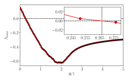
Figure 1: Maximum lyapunov exponent for Izhikevich model with electrical coupling.

The maximum Lyapunov exponent (MLE) of Eq. (10) is presented in Fig. 1. The expanded inset shows that $\Lambda_{max}$ becomes negative for $g_{e}\gamma>0.2670$. To check our results, we simulate a network of $N=2$ nodes, as depicted in Fig. 2. The Laplacian matrix in such case is

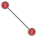
Figure 2: Network with $N=2$ used to verify the result of Fig. 1.

$$L=\begin{bmatrix}1&-1\\ -1&1\end{bmatrix}$$ (11)

with eigenvalues $0$ and $2$, and $\gamma_{2}=2$ is associated with the eigenspace transverse to the synchronized manifold. Putting together that the MLE is negative for $g_{e}\gamma>0.2670$, and that $2$ is the eigenvalue associated with the transverse mode, we conclude that for $g_{e}>0.133$ the synchronized solution is stable.

Fig. 3 depicts the synchronization error, which is computed as $\langle|\mathbf{x}^{1}-\mathbf{x}^{2}|\rangle$, in good agreement with the result given by the MSF.

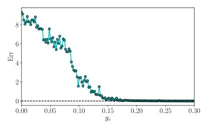
Figure 3: Synchronization error for N=2 with electrical coupling. It goes to zero around $\sigma\approx 0.133$, in conformity with the MSF.

II.2 Chemical coupling

We now study the synchronization of an Izhikevich network with chemical synaptic coupling between nodes. The chemical synapses that node $i$ receives from every other node $j$ are modeled by the sigmodal function $B_{i}$ [30]

$$B_{i}=g_{c}(x^{i}-v_{s})\sum_{j=1}^{N}A_{ij}\zeta(x^{j}),$$ (12)

where $v_{s}$ is the reversal potential, $\zeta(x)=[1+\exp(-\epsilon(x-\theta))]^{-1}$, $\epsilon$ defines the slope of the sigmoidal function and $\theta$ is the synaptic firing threshold. Througout this study we set $v_{s}=20$, $\epsilon=7$ and $\theta=0$. This set of parameters allows the chemical synapses to be both excitatory and inhibitory, since $v_{s}$ lies inside the range of oscillation of the action potential $x_{i}$. This is the case for some classes of neurons, as discussed in [31, 32].

Note that this coupling term cannot be written as a function of the Laplacian matrix, instead we can write it in terms of the adjacency matrix. To obtain an equation analogous to (8), we introduce a few objects, which are defined in the Appendix A, together with the complete derivation of the equation for the dynamics of the network with chemical coupling, which is given by:

$$\mathbf{\dot{x}}=\mathbf{F}(\mathbf{x})-g_{c}\mathbf{T}(\mathbf{x})[(A\otimes\mathbf{C})(\mathbf{x})]\ .$$ (13)

The synchronized solution, $\mathbf{x}^{1}=\mathbf{x}^{2}=...=\mathbf{x}^{N}$, derived in the Appendix A from Eq. (53) to (57), takes the form

$$\mathbf{\dot{x}}^{s}=\mathbf{F}(\mathbf{x}^{s})-g_{c}k_{n}\mathbf{T}(\mathbf{x}^{s})\mathbf{C}(\mathbf{x}^{s})\ ,$$ (14)

and it exists only if the number of links $k_{n}$ is the same for all nodes [33]. Following the Pecora-Carroll analysis, we obtain the Master Stability Function for this case, and after we diagonalize $A$ we have

$$\dot{\eta}=\{[\mathbf{I}_{N}\otimes({D\mathbf{F}\big{|}_{\mathbf{x}^{s}}}-g_{c}k_{n}{D\mathbf{H}\big{|}_{\mathbf{x}^{s}}}\mathbf{K}(\mathbf{x}^{s}))]-g_{c}\Gamma\otimes\mathbf{T}(\mathbf{x}^{s}){D\mathbf{C}\big{|}_{\mathbf{x}^{s}}}\}\eta\ .$$ (15)

The complete derivation of this equation, which is analogous to Eq. (10), is given in Appendix A and it was first derived by Checco et al. [33]. As an example, we consider the network of $N=4$ nodes, depicted in Fig. 4, with an adjacency matrix given by

$$A=\begin{bmatrix}0&1&0&1\\ 1&0&1&0\\ 0&1&0&1\\ 1&0&1&0\end{bmatrix}$$ (16)

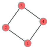
Figure 4: This network, with $N=4$, does not synchronize when the nodes present only chemical coupling, this situation changes when the electrical coupling is added.

The adjacency matrix Eq. (16) has an eigenvalue $\gamma_{1}=2$ associated with the synchronized solution, so we need to calculate the MLE for the remaining eigenvalues $\{0,0,-2\}$. Figure 5 shows the MLE of Eq. (65), which is positive for the range studied. Our calculation for the synchronization error in Fig. (6) shows good agreement with the MLE. The sudden increase in the magnitude of the synchronization error at $g_{c}\approx 0.48$ will be discussed in the context of partial synchronization on Section III.

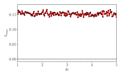
Figure 5: Maximum Lyapunov exponent for Izhikevich model with chemical coupling.

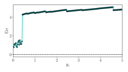
Figure 6: Synchronization error for Izhikevich model with chemical coupling.

II.3 Chemical and electrical coupling

Finally, we study the effect of both electrical and chemical coupling on synchronization. In this case, the evolution of the network is given by

$$\mathbf{\dot{x}}=\mathbf{F}(\mathbf{x})-g_{e}L\otimes\mathbf{G}(\mathbf{x}))-g_{c}\mathbf{T}(\mathbf{x})(A\otimes\mathbf{C})\mathbf{x}\ .$$ (17)

For the sake of simplicity, we consider that both interactions depend on the same diagonalizable adjacency matrix, i.e., $L=D-A$, and that every node has the same number of neighbors $k_{n}$. Combining the results of previous sections, we write the variational equation for the perturbations to the synchronized state as

$$\delta\mathbf{\dot{x}}=\{[\mathbf{I}_{N}\otimes({D\mathbf{F}\big{|}_{\mathbf{x}^{s}}}-g_{c}k_{n}{D\mathbf{H}\big{|}_{\mathbf{x}^{s}}}\mathbf{K}(\mathbf{x}^{s}))]-g_{e}L\otimes{D\mathbf{G}\big{|}_{\mathbf{x}^{s}}}-g_{c}A\otimes\mathbf{T}(\mathbf{x}^{s}){D\mathbf{C}\big{|}_{\mathbf{x}^{s}}}\}\delta\mathbf{x}\ .$$ (18)

Since $L$ and $A$ commute, we can diagonalize both simultaneously, yielding

$$\dot{\eta}=\{[\mathbf{I}_{N}\otimes({D\mathbf{F}\big{|}_{\mathbf{x}^{s}}}-g_{c}k_{n}{D\mathbf{H}\big{|}_{\mathbf{x}^{s}}}\mathbf{K}(\mathbf{x}^{s}))]-[g_{e}\Gamma^{L}\otimes{D\mathbf{G}\big{|}_{\mathbf{x}^{s}}}-g_{c}\Gamma^{A}\otimes\mathbf{T}(\mathbf{x}^{s}){D\mathbf{C}\big{|}_{\mathbf{x}^{s}}}]\}\eta\ .$$ (19)

where $\Gamma^{L}$ and $\Gamma^{A}$ are diagonal matrices with eigenvalues of $L$ and $A$ respectively as entries.

Once again, we take a network of $N=4$ neurons, with electrical and chemical coupling given by $g=g_{e}=g_{c}$ and adjacency matrix (16). Thus, the eigenvalues associated with transverse modes are $\{\gamma^{A}\}=\{0,0,\-2\}$ from the adjacency matrix and $\{\gamma^{L}\}=\{2,2,4\}$, from the Laplacian matrix. We calculate the MLE of Eq. (19) as a function of $g$, and as shown in Fig. (7), the global synchronization pattern becomes stable for $g\approx 0.13$. To confirm this result we calculate the synchronization error over $200$ simulations, which is shown in Fig. 8 and find that it does not go to zero when the MLE becomes negative.

We notice that the synchronization error only vanishes around $g\approx 0.2$, and for values below that, the system can either synchronize or not. Moreover, for $g\approx 0.23$, we see that some simulations yielded a synchronization error greater than expected. To better understand these results, we calculate the synchronization error for different initial conditions, for $g=0.18$ and $g=0.23$. As we see in Fig. 9 (a), for $g=0.18$, depending on the initial conditions, the system can end up in different solutions, a characteristic of multistable systems [34]. Moreover, the different solutions are intertwined in a complex way. This type of basin of attraction is often called a riddled basin, and can be the cause for the divergence between the MLE and the synchronization error results [21].

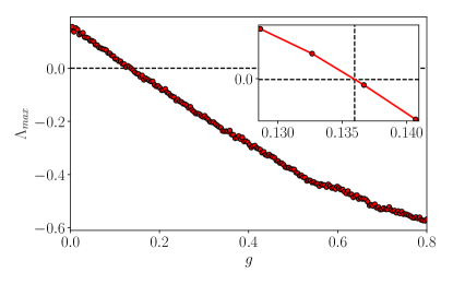
Figure 7: Maximum Lyapunov exponent for Izhikevich model with electrical and chemical coupling.

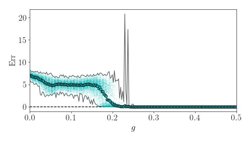
Figure 8: Synchronization error for N=4 with electrical and chemical coupling. The grey lines represent maximum and minimum errors and the circles the average over $200$ simulations.

For $g=0.23$, although the basin of attraction is dominated by synchronized solutions (which represent $96.33\%$ the cases), it is studded with non-synchronized ones, as shown in Fig. 9 (b). Among these cases, few ones yield a synchronization error greater than $15$ ($0.095\%$ of the cases). We verified that in such cases, the network switches from the synchronized solution to a cluster synchronized state with two clusters $(1,3)$ and $(2,4)$ in such a way that these clusters are synchronized but out of phase, resulting in a greater synchronization error. It is worth mentioning that the dynamics of the nodes also changed, as we will discuss later in the text. These results lead us to conclude that the electrical coupling induces synchronization in our network.

Besides that, it is usually assumed that the presence of riddled basins of attraction is related to the MLE approaching zero from below, as discussed in [22, 23]. A similar result, where the system fails to exhibit synchronization when the MLE approaches zeros from above was reported by [21] but the presence of the riddled basin was not investigated.

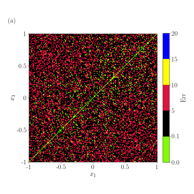
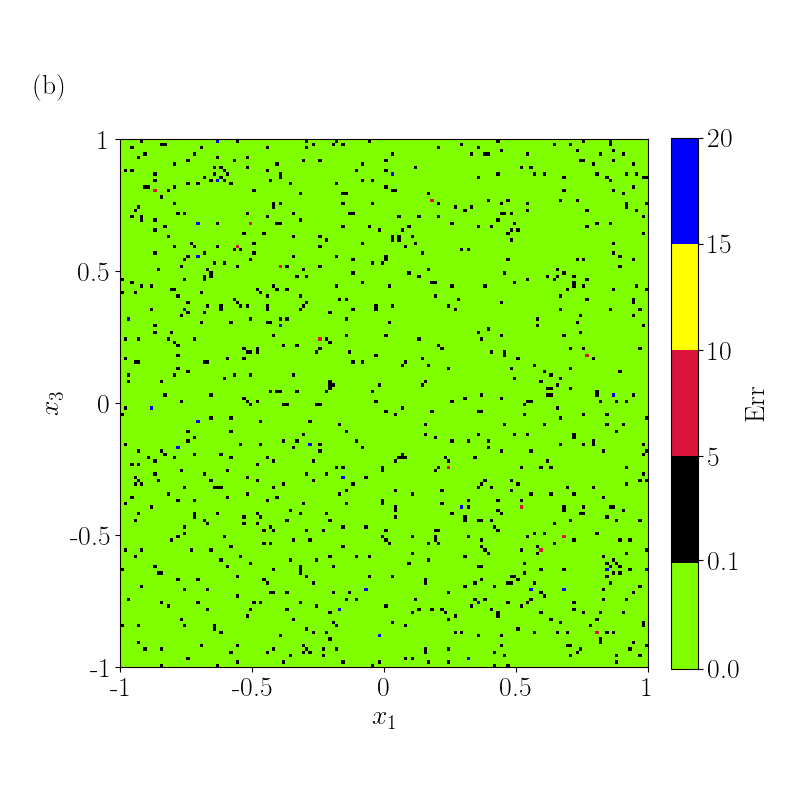
Figure 9: Riddled basin of attraction in $(x_{1},x_{3})$ plane for different values of $g$, calculated with $10.24\times 10^{4}$ initial conditions in $x_{1},x_{3}\in[1,-1]$. (a) is calculated with $g=0.18$. (b) $g=0.23$

III Izhikevich model: Partial Synchronization

III.1 Electrical coupling

As mentioned in the first section, the electrical coupling can be written in terms of the Laplacian matrix. In this case, the variational equation concerning the linear stability around the cluster synchronized state (CSS) is given by [16]

$$\delta\dot{\mathbf{x}}=[\sum_{m=1}^{M}(E^{m}\otimes{D\mathbf{F}\big{|}_{\mathbf{s}^{m}}}-g_{e}(LE^{m}\otimes{D\mathbf{G}\big{|}_{\mathbf{s}^{m}}}))]\delta\mathbf{x}$$ (20)

where $M$ is the number of clusters and $E^{m}$ is an $N\times N$ diagonal indicator matrix for each cluster such that $E^{m}_{ii}=1$ if $i$ belongs to cluster $m$, and it is equal to zero otherwise. If we consider a CSS with $M$ clusters, the dynamical evolution of such state is given by [17, 18]

$$\dot{\mathbf{x}} =(Z\otimes\mathbf{I}_{q})\dot{\mathbf{s}},\quad\text{where}$$ (21)

$$\dot{\mathbf{s}} =\mathbf{F}(\mathbf{s})-g_{e}(L^{\pi}\otimes\mathbf{I}_{q})\mathbf{G}(\mathbf{s})$$ (22)

and $Z$ is the $N\times M$ indicator matrix which encodes the cluster state configuration $Z:Z_{ij}=1$ if node $i$ is part of cluster $C_{j}$ and $Z_{ij}=0$ otherwise. $\mathbf{I}_{q}$ is an $q\times q$ identity matrix, where $q$ is the dimension of the isolated dynamical system, $q=2$ in our case. The state of each cluster is encoded in the $M\times q$-dimensional vector $\mathbf{s}$. If the quotient network Laplacian $L^{\pi}$ satisfies the condition [35]

$$LZ=ZL^{\pi}\ ,$$ (23)

where $L^{\pi}=(Z^{T})^{-1}Z^{T}LZ=Z^{+}LZ$ and $Z^{+}$ is the left Moore-Penrose of pseudoinverse $Z$ [36, 37], then the partition encoded by $Z$ is said to be an Equitable External Partition (EEP) [35]. In this case, the network is divided into $M$ clusters in such way that the number of connections from nodes in a cluster $C_{i}$ to nodes in a cluster $C_{j}$ depends only on $i,j$ with $i\neq j$. The quotient network dynamics is a coarse-grained version of the original network, where each cluster becomes a node and the weights between these nodes are the out-degrees between clusters in the original network [38, 18].

Again, we start our example with a network of Izhikevich neurons coupled through electrical synapses. Consider a network with the following Laplacian matrix

$$L=\begin{bmatrix}2&\-1&0&\-1&0&0&0&0\\ \-1&2&0&\-1&0&0&0&0\\ 0&0&1&\-1&0&0&0&0\\ \-1&\-1&\-1&5&\-1&\-1&0&0\\ 0&0&0&\-1&3&0&\-1&\-1\\ 0&0&0&\-1&0&3&\-1&\-1\\ 0&0&0&0&\-1&\-1&3&\-1\\ 0&0&0&0&\-1&\-1&\-1&3\end{bmatrix}\$$ (24)

and a CSS with indicator matrix $Z$ given by

$$Z=\begin{bmatrix}1&0&0&0&0\\ 1&0&0&0&0\\ 0&1&0&0&0\\ 0&0&1&0&0\\ 0&0&0&1&0\\ 0&0&0&1&0\\ 0&0&0&0&1\\ 0&0&0&0&1\\ \end{bmatrix}\ .$$ (25)

One can verify that this choice of $L$ and $Z$ satisfies (23) and therefore this cluster configuration is an EEP. A representation of such network is given in Fig. 10, where nodes of the same color represent a cluster. Putting this together, Eq. (22) reads

$$[\dot{\mathbf{x}}]^{T}=[\dot{\mathbf{s}}^{1},\dot{\mathbf{s}}^{1},\dot{\mathbf{s}}^{3},\dot{\mathbf{s}}^{4},\dot{\mathbf{s}}^{5},\dot{\mathbf{s}}^{5},\dot{\mathbf{s}}^{7},\dot{\mathbf{s}}^{7}]^{T}\ .$$ (26)

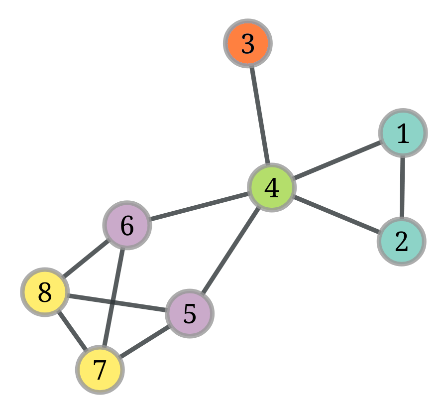
Figure 10: Network studied in this section, where the clusters are indicated with colors.

After block-diagonalizing the variational equation (20), we investigated the linear stability of the CSS with the following equation

$$\mathbf{\dot{\eta}}=\Big{[}\sum_{m}Q^{m}\otimes{D\mathbf{F}\big{|}_{\mathbf{s}^{m}}}-g_{e}\Gamma^{L}Q^{m}\otimes{D\mathbf{G}\big{|}_{\mathbf{s}^{m}}}\Big{]}\mathbf{\eta}\ .$$ (27)

Where $Q^{m}=V^{-1}E^{m}V$ is a block diagonal matrix and $\Gamma^{L}=V^{-1}LV$ is a diagonal matrix filled with eigenvalues of $L$. The orthogonal matrix that block-diagonalizes both ${E^{m}}$ and $L$ can be found using group theory [17], External Equitable Partitions (EEP’s) [18] and Simultaneous Block Diagonalization (SBD) [19] approaches, resulting in the decoupling between modes within the cluster synchronized manifold and transverse to it.

To check if all transverse modes are damped, we calculated the maximum Lyapunov exponent of Eq. (27), which is given in Fig. 11 as a function of $g_{e}$.

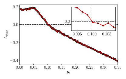
Figure 11: Maximum Lyapunov exponent for Izhikevich model with electrical coupling under partial synchronization.

Fig. 12 shows the synchronization error of the cluster synchronization state as a function of $g_{e}$. The error is computed as $\langle|x^{i}(t)-x_{m}^{i}(t)|\rangle$, where we take an average both in time and over the neurons $i$ in a cluster $m$. $x_{m}^{i}$ is the average state for the neurons in the cluster to which node $i$ belongs.

Fig. 11 and Fig. 12 show excellent agreement between the stability analysis and the synchronization error: the MLE associated with the transverse modes goes negative around $g_{e}\approx 0.10$, and the synchronization error vanishes around the same value.

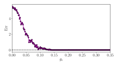
Figure 12: Synchronization error for Izhikevich model with electrical coupling, partial synchronization.

III.2 Chemical coupling

We now extend the linear stability study of cluster synchronized states to networks with chemical coupling, which is mediated by the adjacency matrix of the network. Consider a network with $N$ nodes and adjacency matrix $A$, given a CSS with $M$ clusters encoded by an indicator matrix $Z$, the coarse-grained dynamics can be written as follows

$$\dot{\mathbf{x}} =(Z\otimes\mathbf{I}_{q})\dot{\mathbf{s}},\quad\text{where}$$ (28)

$$\dot{\mathbf{s}} =\mathbf{F}(\mathbf{s})+g_{e}\mathbf{T}(\mathbf{s})(A^{\pi}\otimes\mathbf{C})(\mathbf{s})\ .$$ (29)

If the adjacency matrix of the quotient network is given by $A^{\pi}=Z^{+}AZ$, its diagonal entries corresponds to self-loops in the quotient network whenever we have connections between nodes in the same cluster, and the partition enconded by $Z$ is an External Partition (EP). For EPs the number of connections from nodes in a cluster $C_{i}$ to nodes in a cluster $C_{j}$ depends only in $i,j$ [18].

The variational equation of Eq.(28) is

$${\delta\dot{\mathbf{x}}}=\big{\{}\sum_{m=1}^{M}[E^{m}\otimes({D\mathbf{F}\big{|}_{\mathbf{s}^{m}}}-g_{c}PR^{m})]-[\sum_{m=1}^{M}(E^{m}A\otimes\mathbf{T}(\mathbf{s}^{m}))(\sum_{m=1}^{M}E^{m}\otimes{D\mathbf{K}\big{|}_{\mathbf{s}^{m}}})]\big{\}}\delta\mathbf{x}\ .$$ (30)

And after block-diagonalizing Eq. (30), we obtain

$$\dot{\eta}=\big{\{}\sum_{m=1}^{M}Q^{m}\otimes[{D\mathbf{F}\big{|}_{\mathbf{s}^{m}}}-g_{c}\mathbf{G}R^{m}]-(Q^{m}\Gamma^{A}\otimes\mathbf{T}(\mathbf{s}^{m})(\sum_{m=1}^{M}Q^{m}\otimes{D\mathbf{K}\big{|}_{\mathbf{s}^{m}}})\big{\}}\eta\ .$$ (31)

where we defined

$$\mathbf{G}=\begin{bmatrix}1&0\\ 0&0\end{bmatrix}\quad\text{and}\quad R^{m}=\sum_{n=1}^{M}A^{\pi}_{mn}\zeta(x_{n})\ .$$ (32)

Once again, we consider the network represented in Fig. 4, but now we look for the stability of a CSS, which can explain the sudden increase in the synchronization error around $g_{c}\approx 0.48$ in Fig. 6. The CSS is encoded by the indicator and quotient adjacency matrices, which are given by

$$Z=\begin{bmatrix}1&0\\ 0&1\\ 1&0\\ 0&1\\ \end{bmatrix}\quad\text{and}\quad A^{\pi}=\begin{bmatrix}0&2\\ 2&0\\ \end{bmatrix}\ .$$ (33)

The linear stability analysis of such CSS is given in Fig. 13, where we notice that the CSS becomes stable for $g_{c}>0.53$, which is around the value for which the synchronization error suddenly increases in Fig. 6. This can be explained because the network dynamics are similar to one composed of $N=2$ neurons out-of-phase. Figure 14 shows the synchronization error of the CSS in question, which confirms our stability analysis.

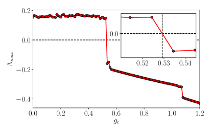
Figure 13: Maximum Lyapunov exponent for Izhikevich model with chemical coupling partial synchronization (N=4).

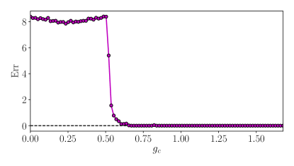
Figure 14: Synchronization error for Izhikevich model with chemical coupling, partial synchronization (N=4).

We now consider the network of the previous subsection, depicted in Fig. 10, and the same indicator matrix $Z$ (Eq. (25)), with chemical coupling between neurons. In this case, the adjacency matrix is given by

$$A=\begin{bmatrix}0&1&0&1&0&0&0&0\\ 1&0&0&1&0&0&0&0\\ 0&0&0&1&0&0&0&0\\ 1&1&1&0&1&1&0&0\\ 0&0&0&1&0&0&1&1\\ 0&0&0&1&0&0&1&1\\ 0&0&0&0&1&1&0&1\\ 0&0&0&0&1&1&1&0\\ \end{bmatrix}\ .$$ (34)

Unlike the case with electrical coupling, here the CSS is not stable, as seen in Fig. (15), where the maximum Lyapunov exponent is positive in the range of $g_{c}$ considered. This analysis is supported by the synchronization error of this case (Fig. 16), which is greater than $0$ in the range of $g_{c}$ studied.

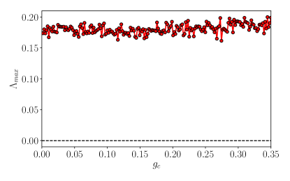
Figure 15: Maximum Lyapunov exponent for Izhikevich model with chemical coupling partial synchronization (N=8).

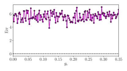
Figure 16: Synchronization error for Izhikevich model with chemical coupling, partial synchronization (N=8).

III.3 Electrical and chemical coupling

In the case where the network admits both eletrical and chemical coupling, the dynamics of the CSS is governed by

$$\dot{\mathbf{x}}= (Z\otimes\mathbf{I}_{q})\dot{\mathbf{s}},\quad\text{where}$$ (35)

$$\dot{\mathbf{s}}=\mathbf{F}(\mathbf{s})-g_{c}\mathbf{T}(\mathbf{s}) (A^{\pi}\otimes\mathbf{C})(\mathbf{s})-g_{e}(L^{\pi}\otimes\mathbf{I}_{q})\mathbf{G}(\mathbf{s})\ .$$ (36)

where $Z$ is the indicator matrix of the CSS state, $A^{\pi}$ and $L^{\pi}$ are the quotient adjacency and Laplacian matrices, and for the sake of simplicity we take $g_{c}=g_{e}=g$. Putting together the results of the later subsections, the master stability function of a given CSS state can be written as

$$\dot{\eta}=\big{\{}\sum_{m=1}^{M}Q^{m}\otimes[{D\mathbf{F}\big{|}_{\mathbf{x}^{m}}}-g_{c}\mathbf{G}R^{m}]-g_{c}(\sum_{m=1}^{M}Q^{m}\Gamma^{A}\otimes\mathbf{T}(\mathbf{x}^{m})(\sum_{m=1}^{M}Q^{m}\otimes{D\mathbf{K}\big{|}_{\mathbf{x}^{m}}})-g_{e}\sum_{m=1}^{M}\Gamma^{L}Q^{m}\otimes{D\mathbf{H}\big{|}_{\mathbf{x}^{m}}}\big{\}}\eta\ .$$ (37)

We proceed with the analysis of the network in Fig. 10, with indicator matrix (25). The MLE of Eq. (37) is shown in Fig. 17, where we notice that the introduction of electrical coupling in the network seems to induce the CSS, since the MLE becomes negative for $g>0.172$.

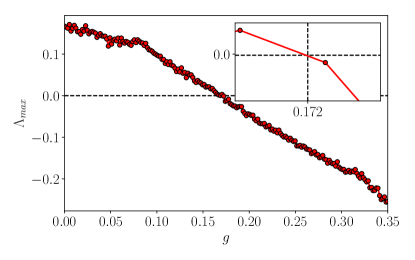
Figure 17: Maximum Lyapunov exponent for the Izhikevich model with chemical and electric coupling, partial synchronization (N=8).

The initial conditions, used to make Fig. 18 (nearly identical but random), were equivalent to adding perturbations to all three directions transverse to the synchronized solution, plus the five directions parallel to the synchronized solution. The dotted line represents the average over $100$ simulations and the shaded area the error bars of these simulations. Although the lower bound of the synchronization error goes to zero around $g\approx 0.172$, we see that on average the system does not reach the synchronized solution. This sensibility to perturbations is characteristic of multistable systems [34], and as discussed in [21], a riddled basin of attraction can be the cause for such behavior, which in turn may be a consequence of the discontinuity of the differential equation. A thorough understanding of this phenomenae needs an intense research which is outside the scope of this work.

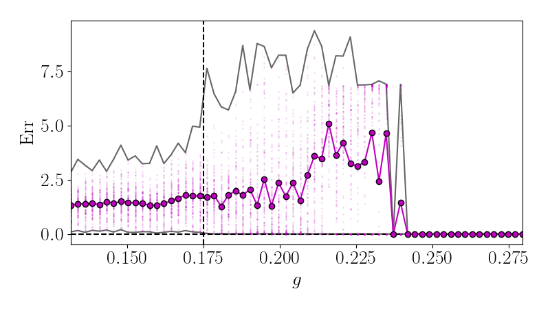
Figure 18: Synchronization error as a function of $g$ for Izhikevich model with electrical and chemical coupling. The CSS considered is the one Fig. 10. The average over $150$ runs, with nearly identical initial conditions, is depicted with its bounds.

To verify that, we consider adding a disturbance in only one direction transverse to the synchronized solution, which means perturbing only one cluster. For example, if we take the solution

$$\mathbf{x}=\begin{bmatrix}\mathbf{s}_{1}\\ \mathbf{s}_{1}\\ \mathbf{s}_{3}\\ \mathbf{s}_{4}\\ \mathbf{s}_{5}\\ \mathbf{s}_{5}\\ \mathbf{s}_{7}\\ \mathbf{s}_{7}\end{bmatrix}\ ,\quad\text{and add}\quad\mathbf{p}_{\perp}=\alpha\begin{bmatrix}1\\ \-1\\ 0\\ 0\\ 0\\ 0\\ 0\\ 0\end{bmatrix}\ \otimes\begin{bmatrix}1\\ 1\end{bmatrix},$$ (38)

where $\alpha$ is a constant used to control the magnitude of the perturbation $\mathbf{p}_{\perp}$, we are pulling the first cluster out of synchronicity. Fig. 19 (a) shows how the synchronization error, represented by colors, is sensible to initial conditions, for $g=0.18$. In this case, we consider initial conditions slightly perturbed as in Eq. (38). The initial conditions for $\mathbf{x}_{(1,2)}=[x^{(1,2)},y^{(1,2)}]^{T}$ vary from $[1,1]$ to $[\-1,\-1]$, which is equivalent to $\alpha$ varying from $1$ to $-1$ in Eq. (38). Along the diagonal $\mathbf{x}_{1}=\mathbf{x}_{2}$ and the system is always synchronized. In the off-diagonal region, we have both synchronized and non-synchronized solutions. The basin is riddled with these two kinds of solutions, which receive different colors depending on the value of the synchronization error. The same calculation is shown in Fig. 19 (b), which shows a zoom on the center of Fig. 19 (a).

This broad error range is due to the different types of solutions that the system allows. In Fig. 20 we show the time-series of the two first nodes in red and blue lines. In Fig. 20(a), a synchronized solution, which yields Err = $0$ (taking into account only $x_{1}$ and $x_{2}$), for (b) and (c) the synchronization error is equal to $2.059$ and $7.964$. The larger synchronization error comes from the last type of solution, depicted in (d), where the two nodes are out of phase, resulting in an Err $=20.884$. In addition to that, in the last case we notice a hard increase in the frequency of spikes.

Fig. 21 depicts the attractors of five different solutions color-coded in the same fashion of Fig. 19. The attractors corresponding to solutions with Err $\leq 10$ are superposed in the same region, while the yellow and blue attractor, which yields an Err between $10$ and $20$, are far apart and have different shape.

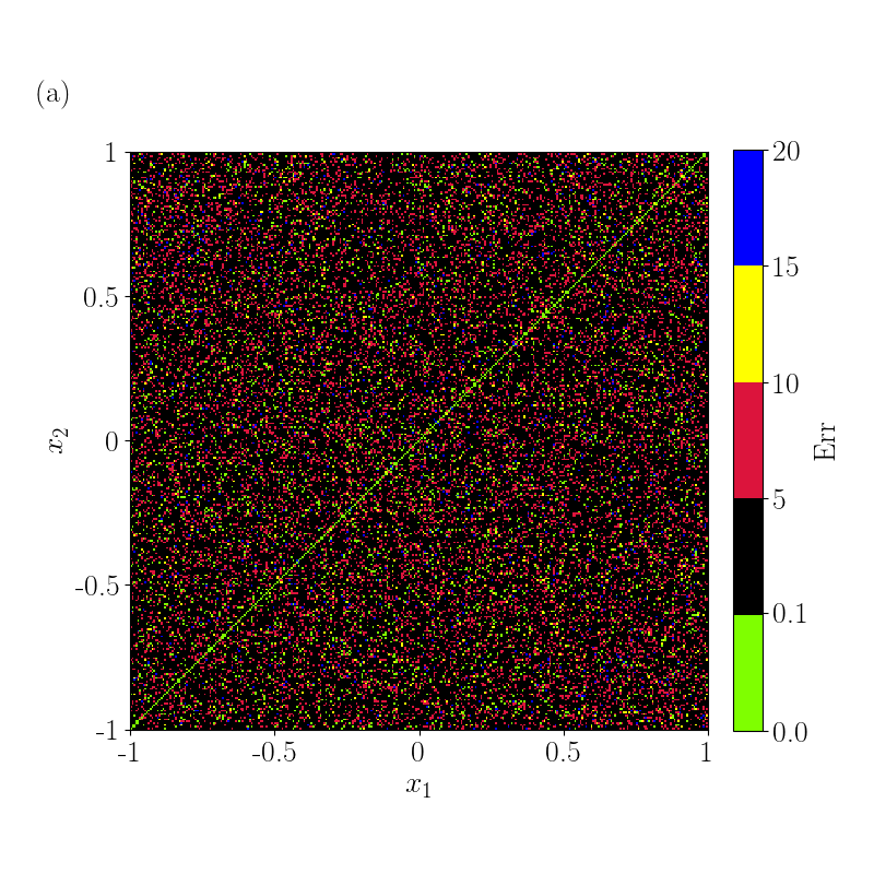
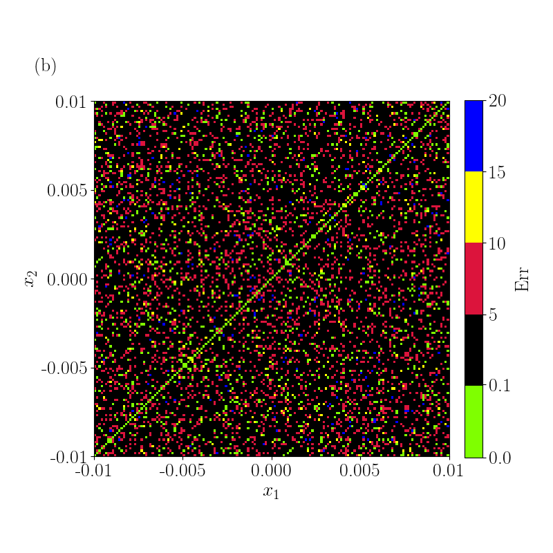
Figure 19: Riddled basin of attraction in $(x_{1},x_{2})$ plane for $g=0.18$. (a) is calculated with $10.24\times 10^{4}$ initial conditions in $x_{1},y_{1}\in[1,-1]$. (b) Inset of (a), calculated with $2.56\times 10^{4}$ initial conditions in $x_{1},y_{1}\in[0.01,-0.01]$.

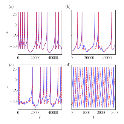
Figure 20: Time series of the $x$-variable from nodes $1$ (red) and $2$ (blue) for different initial conditions. (a) Complete synchronization with Err $=0$, (b) and (c) burst synchronization with Err $=2.05$ and Err $=7.96$, and (d) out of phase synchronization with Err $=20.88$.

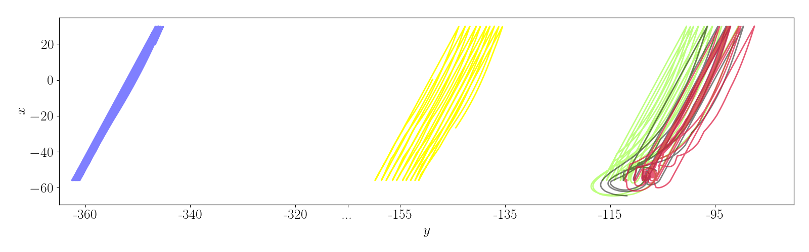
Figure 21: Depending on the initial conditions the system settles into different attractors. Each attractor is color-coded according to the synchronization error in Fig. 19.

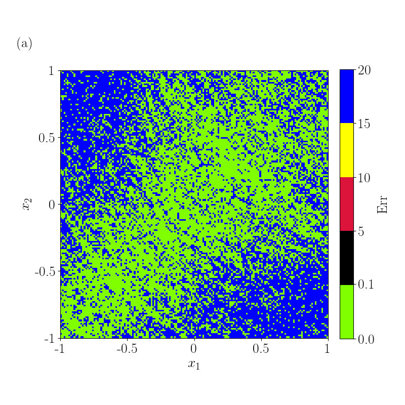
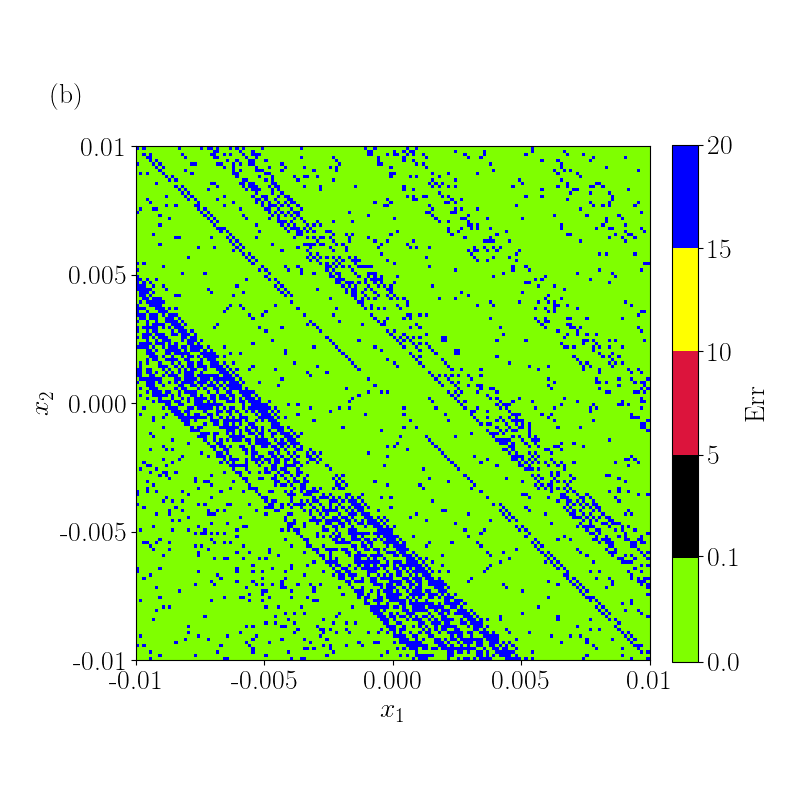
Figure 22: Riddled basin of attraction in $(x_{1},x_{2})$ plane for $g=0.26$. (a) is calculated with $2.56\times 10^{4}$ initial conditions in $x_{1},y_{1}\in[1,-1]$. (b) Inset of (a), calculated with $2.56\times 10^{4}$ initial conditions in $x_{1},y_{1}\in[0.01,-0.01]$.

It is worth mentioning that the transition to synchronization observed in Fig. 18 is due to the nearly identical initial conditions. Taking $g=0.26$, and using initial conditions as in Fig. 22, yields a bistable system, as we see in Fig. 22 (a) and (b). Instead of complete synchronization (Fig. 18) or multiple solutions Fig. (19), in this case, the system is either in a completely synchronized (Err $\approx 0$) or in an out of phase synchronized (Err $\approx 20$) state. The inset in Fig. 22(b) shows that points from these two attractors are interwoven in a riddled fashion.

IV Conclusions

We have calculated the MSF of networks of Izhikevich neurons, considering global and cluster synchronized states with electrical and chemical coupling schemes. To do so, we combined the MSF formalism with the use of saltation matrices, which allow the calculation of Lyapunov exponents of systems with discontinuities such as the Izhikevich model. For the networks studied, we found that the addition of electrical coupling to a network with only chemical coupling induces synchronization for both global and cluster synchronized states. However, the presence of both coupling schemes yielded a riddled basin of attraction. Due to this, even in the range where the MSF is negative and with nearly identical initial conditions concerning the CSS, the system can end up in a not synchronized state and with a different kind of dynamics.

It will be interesting, for future work, to study not only networks with more elements but also how the stability of synchronized solutions if we consider non-identical neurons and the presence of noise in the network. It would also be appealing to investigate why the riddled basins displayed by these systems appear as the MLE approaches zero from above, and not from below as it is usually reported in the literature.

V Acknowledgements

We acknowledge useful discussions with Federico Bizzarri, Bruno Boaretto and Eleonora Catsigeras. R.P.A. acknowledges financing from Coordenação de Aperfeiçoamento de Pessoal de Nível Superior – Brasil (CAPES), Finance Code 001. H.A.C. thanks ICTP-SAIFR and FAPESP Grant No. 2016/01343-7 for partial support.

Appendix A Derivation of MSF for the chemical coupling

Starting from Eq. 12 we define the $2\times 2$ matrices

$$\mathbf{H}=\begin{bmatrix}h&0\\ 0&0\end{bmatrix}\quad\text{and}\quad\mathbf{C}=\begin{bmatrix}\zeta&0\\ 0&0\end{bmatrix}\ ,$$ (39)

where $h$ and $\zeta$ are nonlinear operators

$$hx =h(x)=x-v_{s}\ ,$$ (40)

$$\zeta x=\zeta(x) =[1+\exp(-\epsilon(x-\theta))]^{-1}\ ,$$ (41)

and an operator $\mathbf{Dg}$, that returns a diagonal matrix whose elements are the components of the vector on which it acts. For example, for $\mathbf{x}$:

$$\mathbf{Dg}(\mathbf{x})=\mathbf{Dg}\begin{bmatrix}x^{1}\\ y^{1}\\ \vdots\\ x^{N}\\ y^{N}\end{bmatrix}=\begin{bmatrix}x^{1}&0&...&0&0\\ 0&y^{1}&...&0&0\\ \vdots&\vdots&\ddots&\vdots&\vdots\\ 0&0&...&x^{N}&0\\ 0&0&...&0&y^{N}\end{bmatrix}\ ,$$ (42)

where in this notation $\mathbf{Dg}(\mathbf{x})$ reads $\mathbf{Dg}$ acts on $\mathbf{x}$. We can write the vector encoding the synaptic coupling of a network of $N$ nodes as

$$\mathbf{Dg}[(\mathbf{I}_{N}\otimes\mathbf{H})(\mathbf{x})](A\otimes\mathbf{C})(\mathbf{x})\ .$$ (43)

Moreover, it is convenient to introduce the matrices

$$\mathbf{T}=\mathbf{Dg}(\mathbf{I}_{N}\otimes\mathbf{H})$$ (44)

$$\mathbf{K}=\mathbf{Dg}(\mathbf{I}_{N}\otimes\mathbf{C})\ .$$ (45)

With this notation, the dynamics of a network coupled through chemical synapses reads

$$\mathbf{\dot{x}}=\mathbf{F}(\mathbf{x})-g_{c}\mathbf{T}\mathbf{x}[(A\otimes\mathbf{C})(\mathbf{x})]\ .$$ (46)

For example, if $N=1$,

$$\mathbf{T}\mathbf{x}=\mathbf{Dg}\Bigg{[}\Bigg{(}\mathbf{I}_{1}\otimes\begin{bmatrix}h&0\\ 0&0\end{bmatrix}\Bigg{)}\begin{bmatrix}x^{1}\\ y^{1}\end{bmatrix}\Bigg{]}=\mathbf{Dg}\begin{bmatrix}h(x^{1})\\ 0\end{bmatrix}$$

$$=\begin{bmatrix}x^{1}-v_{s}&0\\ 0&0\end{bmatrix}$$ (47)

If we consider a network with $N=2$ neurons and adjacency matrix given by

$$A=\begin{bmatrix}0&1\\ 1&0\end{bmatrix}\ ,$$ (48)

the coupling term reads

$$\mathbf{T}\mathbf{x} =\mathbf{Dg}\Bigg{(}\begin{bmatrix}1&0\\ 0&1\end{bmatrix}\otimes\begin{bmatrix}h&0\\ 0&0\end{bmatrix}\Bigg{)}\begin{bmatrix}x^{1}\\ y^{1}\\ x^{2}\\ y^{2}\\ \end{bmatrix}=\mathbf{Dg}\begin{bmatrix}h&0&0&0\\ 0&0&0&0\\ 0&0&h&0\\ 0&0&0&0\\ \end{bmatrix}\begin{bmatrix}x^{1}\\ y^{1}\\ x^{2}\\ y^{2}\\ \end{bmatrix}$$

$$\mathbf{Tx} =\mathbf{Dg}\begin{bmatrix}h(x^{1})\\ 0\\ h(x^{2})\\ 0\\ \end{bmatrix}=\begin{bmatrix}h(x^{1})&0&0&0\\ 0&0&0&0\\ 0&0&h(x^{2})&0\\ 0&0&0&0\\ \end{bmatrix}$$ (49)

times

$$(A\otimes\mathbf{C})(\mathbf{x})=\begin{bmatrix}0&0&\zeta&0\\ 0&0&0&0\\ \zeta&0&0&0\\ 0&0&0&0\\ \end{bmatrix}\begin{bmatrix}x^{1}\\ y^{1}\\ x^{2}\\ y^{2}\\ \end{bmatrix}=\begin{bmatrix}\zeta(x^{2})\\ 0\\ \zeta(x^{1})\\ 0\\ \end{bmatrix}$$ (50)

yielding

$$\mathbf{T}(\mathbf{x})[(A\otimes\mathbf{C})(\mathbf{x})] =\begin{bmatrix}h(x^{1})&0&0&0\\ 0&0&0&0\\ 0&0&h(x^{2})&0\\ 0&0&0&0\\ \end{bmatrix}\begin{bmatrix}\zeta(x^{2})\\ 0\\ \zeta(x^{1})\\ 0\\ \end{bmatrix}$$ (51)

$$\mathbf{T}(\mathbf{x})[(A\otimes\mathbf{C})(\mathbf{x})] =\begin{bmatrix}h(x^{1})\zeta(x^{2})\\ 0\\ h(x^{2})\zeta(x^{1})\\ 0\\ \end{bmatrix}\ .$$ (52)

Following the Pecora-Carroll analysis, the master stability function can be obtained via the variational equation for $\delta\mathbf{x}^{i}=\mathbf{x}^{i}-\mathbf{x}^{s}$. So first, we derive the synchronized solution $\mathbf{x}^{s}$, where $\mathbf{x}^{i}=\mathbf{x}^{j}$, $\forall$ $i,j$. If we take an adjacency matrix equal to Eq. 16, we have

$$\mathbf{\dot{x}}^{s}=\mathbf{F}(\mathbf{x}^{s})-g_{c}\mathbf{T}(\mathbf{x}^{s})[(A\otimes\mathbf{C})(\mathbf{x}^{s})]\ ,$$ (53)

the second term reads

$$\mathbf{Dg}\Bigg{\{}\Bigg{(}\begin{bmatrix}1&0&0&0\\ 0&1&0&0\\ 0&0&1&0\\ 0&0&0&1\end{bmatrix}\otimes\begin{bmatrix}h&0\\ 0&0\end{bmatrix}\Bigg{)}\begin{bmatrix}x^{s}\\ y^{s}\\ \vdots\\ x^{s}\\ y^{s}\\ \end{bmatrix}\Bigg{\}}\Bigg{\{}\Bigg{(}\begin{bmatrix}0&1&0&1\\ 1&0&1&0\\ 0&1&0&1\\ 1&0&1&0\end{bmatrix}\otimes\begin{bmatrix}\zeta&0\\ 0&0\end{bmatrix}\Bigg{)}\begin{bmatrix}x^{s}\\ y^{s}\\ \vdots\\ x^{s}\\ y^{s}\end{bmatrix}\Bigg{\}}$$ (54)

which, after application of $\mathbf{Dg}$ becomes:

$$g_{c}\begin{bmatrix}h(x^{s})&0&0&0&0&0&0&0\\ 0&0&0&0&0&0&0&0\\ 0&0&h(x^{s})&0&0&0&0&0\\ 0&0&0&0&0&0&0&0\\ 0&0&0&0&h(x^{s})&0&0&0\\ 0&0&0&0&0&0&0&0\\ 0&0&0&0&0&0&h(x^{s})&0\\ 0&0&0&0&0&0&0&0\\ \end{bmatrix}\Bigg{(}\begin{bmatrix}0&1&0&1\\ 1&0&1&0\\ 0&1&0&1\\ 1&0&1&0\end{bmatrix}\otimes\begin{bmatrix}\zeta&0\\ 0&0\end{bmatrix}\begin{bmatrix}x^{s}\\ y^{s}\\ \vdots\\ x^{s}\\ y^{s}\end{bmatrix}\Bigg{)}$$ (55)

simplifying we obtain:

$$g_{c}\begin{bmatrix}h(x^{s})&0&0&0&0&0&0&0\\ 0&0&0&0&0&0&0&0\\ 0&0&h(x^{s})&0&0&0&0&0\\ 0&0&0&0&0&0&0&0\\ 0&0&0&0&h(x^{s})&0&0&0\\ 0&0&0&0&0&0&0&0\\ 0&0&0&0&0&0&h(x^{s})&0\\ 0&0&0&0&0&0&0&0\\ \end{bmatrix}\begin{bmatrix}\zeta(x^{s})+\zeta(x^{s})\\ 0\\ \zeta(x^{s})+\zeta(x^{s})\\ 0\\ \zeta(x^{s})+\zeta(x^{s})\\ 0\\ \zeta(x^{s})+\zeta(x^{s})\\ 0\\ \end{bmatrix}$$ (56)

which is symply

$$g_{c}k_{n}\mathbf{T}(\mathbf{x}^{s})\mathbf{C}(\mathbf{x}^{s})$$ (57)

where in this case, the number of links that each node has is $k_{n}=2$. Now, we linearize $\mathbf{x}^{i}$ around the synchronized state $\mathbf{x}^{s}$

$$\mathbf{x}^{i}\approx\mathbf{F}(\mathbf{x}^{s})+D\mathbf{F}\big{|}_{\mathbf{x}^{s}}\delta\mathbf{x}^{i}-g_{c}D\Big{[}\mathbf{T}(\mathbf{x}^{i})\sum_{j}a_{ij}\mathbf{C}(\mathbf{x}^{j})\Big{]}\delta\mathbf{x}^{k}\ ,$$ (58)

where $k=(i,j)$ depending on whether the Jacobian matrix $D$ acts on a function of $\mathbf{x}^{i}$ or $\mathbf{x}^{j}$. Evaluating the last term yields

$$D[\mathbf{T}(\mathbf{x}^{i})\sum_{j}a_{ij}\mathbf{C}(\mathbf{x}^{j})]\delta\mathbf{x}^{k}=D\begin{bmatrix}h(x^{i})\sum_{j}a_{ij}\zeta(x^{j})\\ 0\end{bmatrix}\delta\mathbf{x}_{k}$$ (59)

$$=\begin{bmatrix}\frac{\partial h(x^{i})}{\partial x^{i}}\sum_{j}a_{ij}\zeta(x^{j})&0\\ 0&0\end{bmatrix}\delta\mathbf{x}^{i}+\begin{bmatrix}h(x^{i})\sum_{j}a_{ij}\frac{\partial\zeta(x^{j})}{\partial x^{i}}&0\\ 0&0\end{bmatrix}\delta\mathbf{x}^{j}$$ (60)

$$=\begin{bmatrix}\frac{\partial h(x^{i})}{\partial x^{i}}k_{n}\zeta(x^{j})&0\\ 0&0\end{bmatrix}\Bigg{|}_{\mathbf{x}^{s}}\delta\mathbf{x}^{i}+\begin{bmatrix}h(x^{i})\sum_{j}a_{ij}\frac{\partial\zeta(x^{j})}{\partial x^{i}}&0\\ 0&0\end{bmatrix}\Bigg{|}_{\mathbf{x}^{s}}\delta\mathbf{x}^{j}$$ (61)

which is

$$g_{c}k_{n}D\mathbf{H}\big{|}_{\mathbf{x}^{s}}\mathbf{K}(\mathbf{x}^{s})\delta\mathbf{x}^{i}-g_{c}\mathbf{T}(\mathbf{x}^{s})\sum_{j}a_{ij}D\mathbf{C}\big{|}_{\mathbf{x}^{s}}\delta\mathbf{x}^{j}\ .$$ (62)

Then, we can write $\delta\mathbf{x}^{i}$ as

$$\delta\mathbf{x}^{i}=D\mathbf{F}\big{|}_{\mathbf{x}^{s}}-g_{c}k_{n}D\mathbf{H}\big{|}_{\mathbf{x}^{s}}\mathbf{K}(\mathbf{x}^{s})\delta\mathbf{x}^{i}-g_{c}\mathbf{T}(\mathbf{x}^{s})\sum_{j}a_{ij}D\mathbf{C}\big{|}_{\mathbf{x}^{s}}\delta\mathbf{x}^{j}\ .$$ (63)

and finally, we write $\delta\mathbf{x}=[\delta\mathbf{x}^{1},...,\delta\mathbf{x}^{N}]^{T}$ as

$$\delta\dot{\mathbf{x}}=\{[\mathbf{I}_{N}\otimes D\mathbf{F}\big{|}_{\mathbf{x}^{s}}-g_{c}k_{n}D\mathbf{H}\big{|}_{\mathbf{x}^{s}}\mathbf{K}(\mathbf{x}^{s}))]-g_{c}A\otimes\mathbf{T}(\mathbf{x}^{s})D\mathbf{C}\big{|}_{\mathbf{x}^{s}}\}\delta\dot{\mathbf{x}}\ .$$ (64)

The diagonalization of $A$ leads to the desired block diagonalized variational equation:

$$\dot{\eta}=\{[\mathbf{I}_{N}\otimes(D\mathbf{F}\big{|}_{\mathbf{x}^{s}}-g_{c}k_{n}D\mathbf{H}\big{|}_{\mathbf{x}^{s}}\mathbf{K}(\mathbf{x}^{s}))]-g_{c}\Gamma\otimes\mathbf{T}(\mathbf{x}^{s})D\mathbf{C}\big{|}_{\mathbf{x}^{s}}\}\eta\ .$$ (65)

References

- Purves et al. [2009] D. Purves, G. J. Augustine, D. Fitzpatrick, W. C. Hall, A.-S. LaMantia, and R. D. Mooney, Neuroscience (Oxford, 2009).
- Hodgkin and Huxley [1952] A. L. Hodgkin and A. F. Huxley, J. Physiol. 117, 500 (1952).
- Izhikevich [2003] E. M. Izhikevich, IEEE Trans. Neural Net. 14, 1569 (2003).
- Izhikevich and Edelman [2008] E. M. Izhikevich and G. M. Edelman, Proc. Natl. Acad. Sci. U.S.A. 105, 3593 (2008).
- Modolo et al. [2007] J. Modolo, E. Mosekilde, and A. Beuter, J. of Physiol. Paris 101, 56 (2007).
- Buzsaki [2006] G. Buzsaki, Rhythms of the Brain (Oxford University Press, 2006).
- Jiruska et al. [2013] P. Jiruska, M. Curtis, J. G. R. Jefferys, C. A. Schevon, S. J. Schiff, and K. Schindler, J. Physiol. 594, 787 (2013).
- Uhlhaas and Singer [2006] P. Uhlhaas and W. Singer, Neuron 52, 155 (2006).
- Cohen and D’Esposito [2016] J. R. Cohen and M. D’Esposito, J. Neurosci. 36, 12083 (2016).
- Axmacher [2006] N. Axmacher, and F. Mormann, and G. Fernández, and C. E. Elger, and J. Fell Brain. Res. Rev. 52, 170-182 (2006).
- Fries [2009] P. Fries, Annu. Rev. of Neurosci. 32, 209 (2009).
- Pecora and Carroll [1998] L. M. Pecora and T. L. Carroll, Phys. Rev. Lett. 80, 2109 (1998).
- Nishikawa and Motter [2006] T. Nishikawa and A. E. Motter, Phys. Rev. E 73, 065106(R) (2006).
- Sun et al. [2009] J. Sun, E. M. Bollt, and T. Nishikawa, Europhys. Lett. 73, 60011 (2009).
- Rossa et al. [2020] F. D. Rossa, L. Pecora, K. Blaha, A. Shirin, I. Klickstein, and F. Sorrentino, Nat. Commun. 11 (2020).
- Pecora et al. [2014] L. M. Pecora, F. Sorrentino, A. M. Hagerstrom, T. E. Murphy, and R. Roy, Nat. Commun. 5 (2014).
- Pecora et al. [2016] L. M. Pecora, F. Sorrentino, A. M. Hagerstrom, T. E. Murphy, and R. Roy, Sci. Adv. 2 (2016).
- Schaub et al. [2016] M. Schaub, N. O’Clery, Y. N. Billeh, J.-C. Delvenne, R. Lambiotte, and M. Barahona, Chaos 26, 094821 (2016).
- Zhang et al. [2021] Y. Zhang, V. Latora, and A. E. Motter, Commun. Phys. 4 (2021).
- Alexander et al. [1992] J. C. Alexander, J. A. Yorke, Y. Z., and I. Kan, Int. J. Bifurc. Chaos 2, 795 (1992).
- Huang et al. [2009] L. Huang, Q. Chen, Y.-C. Lai, and L. M. Pecora, Phys. Rev. E 80, 036204 (2009).
- Heagy [1994] J. F. Heagy, T. L. Carroll, and L. M. Pecora, Phys. Rev. Lett. 73, (1994).
- Ott [1994] E. Ott, J. C. Sommerer, Phys. Lett. A 188, 39-47 (1994).
- Shimada and Nagashima [1979] I. Shimada and T. Nagashima, Prog. Theor. Phys. 61, 1605 (1979).
- Benettin et al. [1980] G. Benettin, L. Galgani, A. Giorgilli, and J.-M. Strelcyn, Meccanica 15, 9 (1980).
- Wolf et al. [1985] A. Wolf, J. . B. Swift, H. L. Swinney, and J. A. Vastano, Phys. D. 16, 285 (1985).
- Bizzari et al. [2013] F. Bizzari, A. Brambilla, and G. S. Gajani, J. Comput. Neurosci. 35, 201 (2013).
- di Bernardo et al. [2008] M. di Bernardo, C. J. Budd, A. R. Champneys, and P. Kowalczyk, Piecewise-smooth dynamical systems: theory and applications (Springer, 2008) p. 106.
- Perkel et al. [1981] D. H. Perkel, b. Mulloney, and R. W. Budelli, Neuroscience 6, 823 (1981).
- Somers and Kopell [1993] D. Somers and N. Kopell, Biol. Cybern. 68, 393 (1993).
- Root et al. [2014] D. H. Root, C. Mejias-Aponte, S. Zhang, H. Wang, A. F. Hoff, C. R. Lupica, and M. Morales, Nat. Neurosci. 17, 1543 (2014).
- Pelkey et al. [2020] K. A. Pelkey, D. Calvigioni, C. Fang, G. Vargish, T. Ekins, K. Auville, J. C. Wester, M. Lai, C. M.-C. Scott, X. Yuan, S. Hunt, D. Abebe, Q. Xu, J. Dimidschstein, G. Fishell, R. Chittajallu, and C. J. McBain, eLife 9, e51995 (2020).
- Checco et al. [2008] P. Checco, M. Righero, M. Biey, and L. Kocarev, IEEE Trans. Circuits Syst. II 55, 1274 (2008).
- Feudel [2008] U. Feudel, Int. J. Bifurc. Chaos 18, 1607 (2008).
- Cardoso et al. [2007] D. M. Cardoso, C. Delorme, and P. Rama, Eur. J. Comb. 28, 665 (2007).
- Moore [1920] E. H. Moore, Bull. Amer. Math. Soc 26, 394 (1920).
- Penrose [1955] R. Penrose, Math. Proc. Camb. Philos. Soc. 51, 406 (1955).
- O’Clery et al. [2007] N. O’Clery, Y. Yuan, G.-B. Stan, and M. Barahona, Phys. Rev. E 88, 042805 (2007).