Cross-Platform Comparison of Arbitrary Quantum Processes

Abstract

In this work, we present a protocol for comparing the performance of arbitrary quantum processes executed on spatially or temporally disparate quantum platforms using Local Operations and Classical Communication (LOCC). The protocol involves sampling local unitary operators, which are then communicated to each platform via classical communication to construct quantum state preparation and measurement circuits. Subsequently, the local unitary operators are implemented on each platform, resulting in the generation of probability distributions of measurement outcomes. The max process fidelity is estimated from the probability distributions, which ultimately quantifies the relative performance of the quantum processes. Furthermore, we demonstrate that this protocol can be adapted for quantum process tomography. We apply the protocol to compare the performance of five quantum devices from IBM and the "Qianshi" quantum computer from Baidu via the cloud. Remarkably, the experimental results reveal that the protocol can accurately compare the performance of the quantum processes implemented on different quantum computers, requiring significantly fewer measurements than those needed for full quantum process tomography. We view our work as a catalyst for collaborative efforts in cross-platform comparison of quantum computers.

I Introduction

As the field of quantum computing and quantum information gains traction, an increasing number of manufacturers are entering the market, producing their own quantum computers. However, the current generation of noisy intermediate-scale quantum (NISQ) computers, despite their potential, are still hindered by quantum noise [1]. A great challenge is how to compare the performance of the quantum computers fabricated by different manufacturers and located in different laboratories, termed as cross-platform comparison. This task is especially relevant when we move towards regimes where comparing to classical simulations becomes computationally challenging, and therefore a direct comparison of quantum computers is necessary.

A standard method to achieve cross-platform comparison is the quantum tomography [2], in which we first reconstruct the full information of quantum computers under investigation, and then estimate their relative fidelity from the obtained matrices. However, quantum tomography is known to be time consuming and computationally difficult; even learning a few-qubit quantum state is already experimentally challenging [3, 4]. A more efficient way is to estimate the fidelity of the quantum computer without resorting to the full information. Indeed, a variety of estimation and verification tools [5, 6], such as fidelity estimation [7, 8, 9, 10, 11, 12] and quantum verification [13, 14, 15, 16], have been developed along this way. However, these methods assume that one can access a known and theoretical target, usually simulated by classical computers. They quickly become inaccessible for quantum computers containing several hundreds or even thousands of highly entangled qubits, due to the intrinsic time complexity of classical simulation.

Recently, Elben et al. [17] proposed the first cross-platform protocol for estimating the fidelity of quantum states, which are possibly generated by spatially and temporally separated quantum computers. This protocol requires only local measurements in randomized product bases and classical communication between quantum computers. Numerical simulation shows that it consumes significantly fewer measurements than full quantum state tomography. It is expected be applicable in state-of-the-art quantum computers consisting of a few tens of qubits. Later on, Knörzer et al. [18] extended Elben’s protocol to cross-platform comparison of quantum networks, assuming the existence of quantum links that can teleport quantum states. Nevertheless, a quantum link transferring quantum states of many qubits with high accuracy between two distant quantum computers is far from reach in the near future.

In this work, by elaborating the core idea of [17], we present a novel protocol for cross-platform comparing spatially and temporally separated quantum processes. The protocol uses only single-qubit unitary gates and classical communication between quantum computers, without requiring quantum links or ancilla qubits. This approach allows for accurate estimation of the performance of quantum devices manufactured in separate laboratories and companies using different technologies. Furthermore, the protocol can be used to monitor the stable function of target quantum computers over time. We apply the protocol to compare the performance of five quantum devices from IBM and the "Qianshi" quantum computer from Baidu via the cloud. Our experimental results reveal that our protocol can accurately compare the performance of arbitrary quantum processes. Although the sample complexity of our protocol still scales exponentially with the number of qubits, it has a significantly smaller exponent factor compared with that of quantum process tomography. Overall, our protocol serves as a novel application of the powerful randomized measurement toolbox [19].

The rest of the paper is organized as follows. Section II reviews the cross-platform quantum state comparison protocol in [17] and introduces the quantum process performance metric. Section III elaborates the main result, a new protocol for cross-platform comparing arbitrary quantum processes. Particularly, we summarize the similarities and differences between our protocol and that of [18]. Section IV reports a thorough experimental cross-platform comparison on spatially and temporally separated quantum computers, along with a comprehensive investigation of the experimental data. The Appendices summarize technical details of the main text.

II Preliminaries

II.1 Cross-platform comparison of quantum states

In quantum information, fidelity is an important metric that is widely used to characterize the closeness between quantum states. There are many different proposals for the definition of state fidelity [20]. In this work, we will concentrate on the max fidelity, formally defined as [20, 17]

$$F_{\max}(\rho_{1},\rho_{2})\mathrel{\mathop{\mathchar 58\relax}}=\frac{\operatorname{Tr}[\rho_{1}\rho_{2}]}{\max\{\operatorname{Tr}[\rho_{1}^{2}],\operatorname{Tr}[\rho_{2}^{2}]\}},$$ (1)

where $\rho_{i}$ is an $n$-qubit quantum state produced by the quantum computer, $i=1,2$.

Elben et al. [17] proposed a randomized measurement protocol to estimate $F_{\max}$, which functions as follows. First, we construct an $n$-qubit unitary $U=\bigotimes_{k=1}^{n}U_{k}$, where each $U_{k}$ is identically and independently sampled from a single-qubit set $\mathcal{X}_{2}$ satisfying unitary $2$-design [21, 22]. This information will be classically communicated to the quantum computers, possibly spatially or temporally separated, that produce the quantum states $\rho_{1}$ and $\rho_{2}$, respectively. Then, each quantum computer executes the unitary $U$, performs a computational basis measurement, and records the measurement outcome $\bm{s}$. Repeating the above procedure for fixed $U$ a number of times, we are able to obtain two probability distributions over the outcomes of the form $\Pr_{U}^{(1)},\Pr_{U}^{(2)}$, where the superscript $i$ represents that the distribution is obtained from quantum state $\rho_{i}$. Next, we repeat the whole procedure for many different random unitaries $U$, yielding a set of probability distributions $\{\Pr_{U}^{(1)},\Pr_{U}^{(2)}\}_{U}$. From the experimental data, we estimate the overlap between $\rho_{i}$ and $\rho_{j}$ as [17]

$$\operatorname{Tr}[\rho_{i}\rho_{j}]=2^{n}\sum_{\bm{s},\bm{s}^{\prime}\in\{0,1\}^{n}}(-2)^{-\mathcal{D}[\bm{s},\bm{s}^{\prime}]}\overline{{\rm Pr}_{U}^{(i)}[\bm{s}]{\rm Pr}_{U}^{(j)}[\bm{s}^{\prime}]},$$ (2)

where $\overline{\cdots}$ denotes the ensemble average over the sampled unitaries $U$ and $\mathcal{D}[\bm{s},\bm{s}^{\prime}]$ denotes the hamming distance between two bitstrings $\bm{s}$ and $\textbf{s}^{\prime}$. Specially, $\operatorname{Tr}[\rho_{1}\rho_{2}]$ can be estimated from (2) by setting $i=1$ and $j=2$, whereas the purities $\operatorname{Tr}[\rho_{1}^{2}]$ and $\operatorname{Tr}[\rho_{2}^{2}]$ can be obtained by setting $i=j=1$ and $i=j=2$, respectively. Using the above estimated quantities, we successfully compute the max fidelity $F_{\max}(\rho_{1},\rho_{2})$.

Using experimental data from [23], Elben et al. showcased the experiment-theory fidelities and experiment-experiment fidelities of highly entangled quantum states prepared via quench dynamics in a trapped ion quantum simulator as a proof of principle [17]. Recently, Zhu et al. reported thorough cross-platform comparison of quantum states in four ion-trap and five superconducting quantum platforms, with detailed analysis of the results and an intriguing machine learning approach to explore the data [24].

II.2 Quantum process performance metric

A quantum process, also known as a quantum operation or a quantum channel, is a mathematical description of the evolution of a quantum system. It is mathematically formulated as a completely positive and trace-preserving (CPTP) linear map on the quantum states [25]. The Choi-Jamiołkowski isomorphism provides a unique way to represent quantum processes as quantum states in a larger Hilbert space. Formally, the Choi state of an $n$-qubit quantum process $\mathcal{E}$ is defined as [26]

$$\eta_{\mathcal{E}}\mathrel{\mathop{\mathchar 58\relax}}=(\mathcal{I}\otimes\mathcal{E})|{\psi_{+}}\rangle\!\langle{\psi_{+}}|,$$ (3)

where $\mathcal{I}$ is the identity channel and $\left|{\psi_{+}}\right\rangle\mathrel{\mathop{\mathchar 58\relax}}=1/\sqrt{2^{n}}\sum\left|{ii}\right\rangle$ is a maximally entangled state of a bipartite quantum system composed of two $n$-qubit subsystems.

One lesson we can learn from the cross-platform state comparison protocol is that, we must choose a process metric before comparing two quantum processes. Gilchrist et al. [27] have introduced a systematic way to generalize a metric originally defined on quantum states to a corresponding metric on quantum processes, utilizing the Choi-Jamiołkowski isomorphism. Specifically, the max fidelity between two $n$-qubit quantum processes $\mathcal{E}_{1}$ and $\mathcal{E}_{2}$, implemented on different quantum platforms, is defined as

$$F_{\max}(\mathcal{E}_{1},\mathcal{E}_{2})\mathrel{\mathop{\mathchar 58\relax}}=F_{\max}(\eta_{\mathcal{E}_{1}},\eta_{\mathcal{E}_{2}}),$$ (4)

where $\eta_{\mathcal{E}}$ is the Choi state of quantum process $\mathcal{E}$. This metric fulfills the axioms for quantum process fidelities following the argument in [27]. It is reasonable to believe that, at least to some extent, this metric reveals that the quantum processes have implemented the same quantum evolution.

In the following, we propose an experimentally efficient protocol to estimate this metric. This protocol makes use of only single-qubit unitaries and classical communication, thus can be executed in spatially and temporally separated quantum devices. This enables cross-platform comparison of arbitrary quantum processes.

III Cross-Platform Comparison

In this section, we first provide a simple example to illustrate the necessity of cross-platform comparison. Then, we introduce a protocol for estimating the max process fidelity that is conceptually straightforward yet experimentally challenging. Next, we propose a modification to the protocol that employs randomized input states and provide a detailed explanation of the approach. Furthermore, we demonstrate that our protocol can be extended to accomplish full process tomography. Our protocol is motivated by the observation that even identical quantum computers cannot produce identical outcomes on each run due to the intrinsic randomness of quantum mechanics, but they do generate identical probability distributions from a statistical perspective.

Cross-platform comparison of quantum computers is essential for at least two reasons. Firstly, comparing the actual implementation with an idealized theoretical simulation can be challenging, as classical simulations become computationally demanding with an increasing number of qubits. Secondly, due to the presence of varying forms of quantum noise across different quantum platforms, the actual implementation of quantum processes can vary significantly, even if they maintain the same process fidelity with respect to the ideal target. To illustrate this point, consider the following example. Suppose Alice has a superconducting quantum computer and Bob has a trapped-ion quantum computer. They implement the single-qubit Hadamard gate $\mathcal{H}(\rho)=H\rho H^{\dagger}$ on their respective quantum computers. However, Alice’s implementation $\mathcal{E}_{1}$ suffers from the depolarizing noise, yielding $\mathcal{E}_{1}(\rho)=(1-p_{1})H\rho H^{\dagger}+p_{1}\mathbbm{1}/2$, where $p_{1}=7/30$. On the other hand, Bob’s implementation $\mathcal{E}_{2}$ suffers from the dephasing noise, such that $\mathcal{E}_{2}(\rho)=(1-p_{2})H\rho H^{\dagger}+p_{2}{\rm\Delta(\rho)}$, where $p_{2}=1/5$ and $\Delta(\cdot)$ is the dephasing operation. After simple calculations, we obtain $F_{\max}(\mathcal{E}_{1},\mathcal{H})=F_{\max}(\mathcal{E}_{2},\mathcal{H})\approx 0.808$ and $F_{\max}(\mathcal{E}_{1},\mathcal{E}_{2})\approx 0.978$. Despite $\mathcal{E}_{1}$ and $\mathcal{E}_{2}$ having the same fidelity level when compared to the ideal target $\mathcal{H}$, discernible difference exists between them. Therefore, solely comparing the fidelity of a quantum process to an ideal reference is insufficient, and a direct comparison between quantum processes is warranted.

III.1 Ancilla-assisted cross-platform comparison

In this section, we recover a conceptually simple approach for estimating the max process fidelity defined in Eq. (4), which was recently proposed in [18]. The key observation is that this fidelity can be seen as the max state fidelity between the Choi states of the corresponding quantum processes. To construct the Choi state of the $n$-qubit quantum process $\mathcal{E}$, we need to introduce an additional $n$-qubit clean auxiliary system. Using the auxiliary system, we prepare a $2n$-qubit maximally entangled state $|\psi_{+}\rangle$ and apply $\mathcal{E}$ to half of the whole system, which successfully prepares the Choi state of $\mathcal{E}$. We can then estimate the max state fidelity using the procedure introduced in Section II.1. The complete protocol is illustrated in Figure 1(a)-(c).

We refer to this protocol as the ancilla-assisted cross-platform comparison because it requires additional clean ancilla qubits to prepare the Choi state of the quantum process. To perform this protocol, a maximally entangled state is required as input, resulting in a two-fold overhead when comparing $2n$-qubit states instead of $n$-qubit states. Consequently, this protocol may not be practical in scenarios with limited quantum computing resources. Furthermore, preparing high-fidelity maximally entangled states can be experimentally challenging, which may negatively impact the accuracy of the protocol.

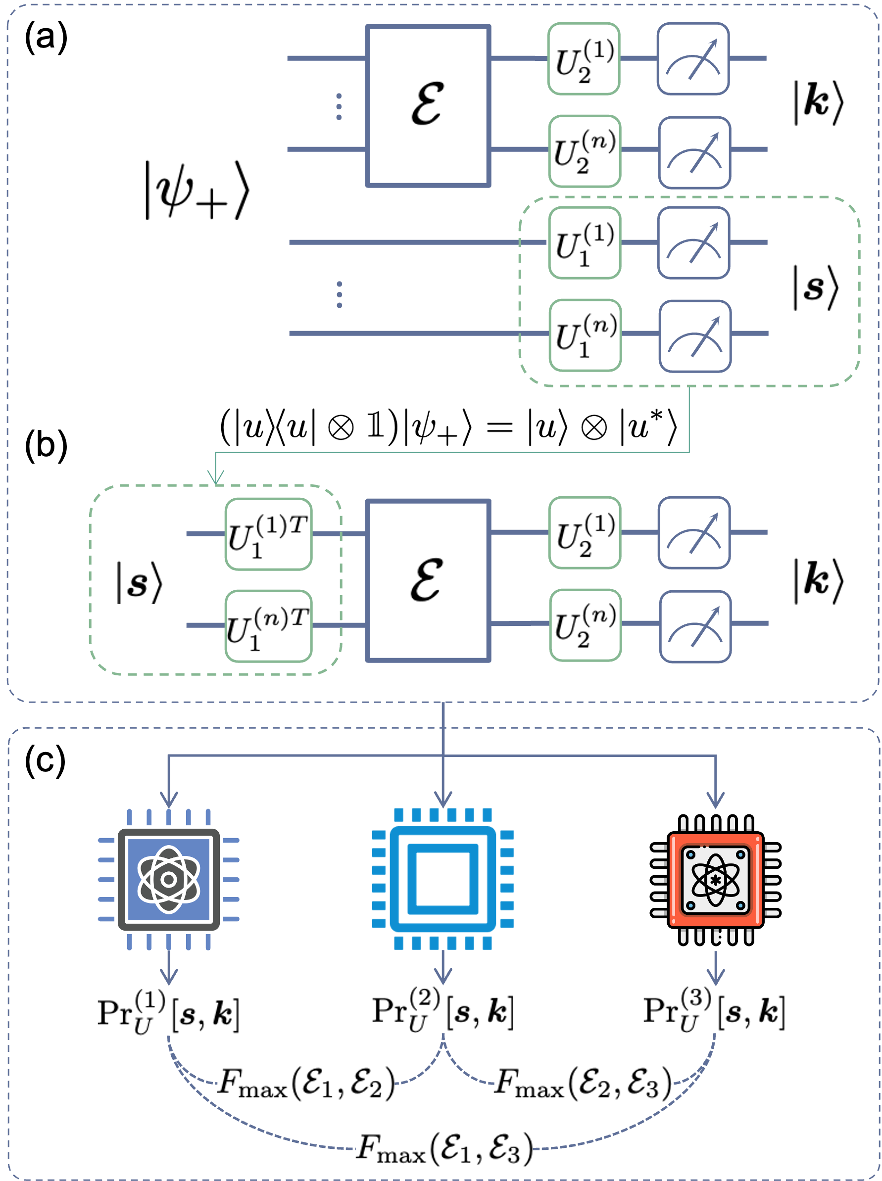
Figure 1: Two protocols to estimate the max process fidelity $F_{\max}$ between quantum processes implemented on different quantum platforms. (a) Ancilla-assisted protocol: Prepare the maximally entangled state, execute the target quantum process, and perform the randomized measurements given by $\otimes_{k=1}^{n}U_{1}^{(k)}\otimes\otimes_{k=1}^{n}U_{2}^{(k)}$. (b) Ancilla-free protocol: Randomly sample a computational basis $\left|{\bm{s}}\right\rangle$, execute the unitaries $\otimes_{k=1}^{n}U_{1}^{(k)T}$, execute the target quantum process, and perform the randomized measurements given by $\otimes_{k=1}^{n}U_{2}^{(k)}$. (c) Run the quantum circuits constructed in (a) or (b) on platform $\mathcal{S}_{i}$ to obtain the probability distribution $\Pr_{U}^{(i)}[\bm{s},\bm{k}]$. The max process fidelity $F_{\max}(\mathcal{E}_{i},\mathcal{E}_{j})$ is inferred from the probability distributions (see text).

III.2 Ancilla-free cross-platform comparison

To overcome the limitations of the ancilla-assisted protocol, we propose an efficient and ancilla-free approach for estimating the max process fidelity. Our protocol does not require any additional qubits or the preparation of maximally entangled states. The key observation is that the auxiliary system in the ancilla-assisted protocol only needs to perform randomized measurements. After the measurement, the auxiliary system collapses to one eigenstate of the sampled measurement operator. Based on the identity $(|{u}\rangle\!\langle{u}|\otimes\mathbbm{1})\left|{\psi_{+}}\right\rangle=\left|{u}\right\rangle\otimes\left|{u^{*}}\right\rangle$, where $\mathbbm{1}$ is the identity matrix, and the deferred measurement principle [28], we can eliminate the auxiliary system by preparing computational states and applying the transposed unitary operator on the main system. Please refer to Appendix A for a detailed analysis.

We refer to the new protocol as the ancilla-free cross-platform comparison and it works as follows. We consider two $n$-qubit quantum processes $\mathcal{E}_{1}$ and $\mathcal{E}_{2}$ realized on different quantum platforms $\mathcal{S}_{1}$ and $\mathcal{S}_{2}$, whose Choi states are $\eta_{1}$ and $\eta_{2}$, respectively. The protocol, illustrated in Figure 1(b)-(c), consists of three main steps: sampling unitaries, running circuits, and post-processing.

Step 1. Sampling unitaries: Construct two $n$-qubit unitaries $U_{i}=\bigotimes_{k=1}^{n}U_{i}^{(k)}$, $i=1,2$, where each $U_{i}^{(k)}$ is identically and independently sampled from a single-qubit set $\mathcal{X}_{2}$ satisfying unitary $2$-design. The information of $U_{i}$ is then communicated to both platforms via classical communication.

Step 2. Running circuits: After receiving the information of the sampled unitaries, Each platform $\mathcal{S}_{i}$ ($i=1,2$) initializes its quantum system to the computational states $\left|{\bm{s}}\right\rangle$ and applies the first unitary $U_{1}$ to $\left|{\bm{s}}\right\rangle$. Subsequently, $\mathcal{S}_{i}$ implements the quantum process $\mathcal{E}_{i}$ and applies the second unitary $U_{2}$. Finally, $\mathcal{S}_{i}$ performs the projective measurement in the computational basis and obtains an outcome $\bm{k}$. Repeating the above procedure many times, we obtain two probability distributions $\Pr_{K|\bm{s},U_{1},U_{2}}^{(1)}$ and $\Pr_{K|\bm{s},U_{1},U_{2}}^{(2)}$ over the measurement outcomes $\bm{k}$ for the fixed computational state $\left|{\bm{s}}\right\rangle$ and unitaries $U_{1}$ and $U_{2}$. By exhausting the computational states and repeatedly sampling the unitaries, we obtain two probability distributions $\Pr_{K,S|U_{1},U_{2}}^{(i)}$ with respect to the sampled unitaries and computational state inputs. For simplicity, we abbreviate $\Pr_{K,S|U_{1},U_{2}}^{(i)}$ to $\Pr^{(i)}_{U}$.

Step 3. Post-processing: From the experimental data, we estimate the overlap between the Choi states $\eta_{i}$ and $\eta_{j}$ for $i,j=1,2$ as

$$\begin{split}\operatorname{Tr}[\eta_{i}\eta_{j}]=4^{n}\sum_{\bm{s},\bm{s}^{\prime},\bm{k},\bm{k}^{\prime}\in\{0,1\}^{n}}&(-2)^{-\mathcal{D}[\bm{s},\bm{s}^{\prime}]-\mathcal{D}[\bm{k},\bm{k}^{\prime}]}\\ &\times\overline{{\rm Pr}^{(i)}_{U}[\bm{s},\bm{k}]{\rm Pr}^{(j)}_{U}[\bm{s}^{\prime},\bm{k}^{\prime}]}.\end{split}$$ (5)

where $\overline{\cdots}$ denotes the ensemble average over the sampled unitaries $U_{1}$ and $U_{2}$. This is proven in Appendix A. By setting $i=1$ and $j=2$, we can estimate the overlap $\operatorname{Tr}[\eta_{1}\eta_{2}]$ from the above equation, which is the second-order cross-correlation of the probabilities $\Pr^{(1)}_{U}$ and $\Pr^{(2)}_{U}$. We can obtain the purities $\operatorname{Tr}[\eta_{1}^{2}]$ and $\operatorname{Tr}[\eta_{2}^{2}]$ by setting $i=j=1$ and $i=j=2$, respectively. These are the second-order autocorrelations of the probabilities. Using the estimated quantities, we compute the max process fidelity $F_{\max}(\mathcal{E}_{1},\mathcal{E}_{2})$ in Eq. (4).

There are several important points to note about our protocol. First, when classical simulation is available, the protocol can be used to compare the experimentally implemented process to the theoretical simulation, providing a useful tool for experiment-theory comparison. Second, our protocol can also estimate the process purity $\operatorname{Tr}[\eta_{\mathcal{E}}^{2}]$ of a quantum process $\mathcal{E}$, which measures the extent to which $\mathcal{E}$ preserves the purity of the quantum state. This is an important measure for characterizing quantum processes, and our protocol provides an efficient way to estimate it. Finally, it is worth noting that the definition of max process fidelity is not unique, and different approaches exist [27, 29]. Our protocol, based on statistical correlations of randomized inputs and measurements, can be readily extended to any metric that depends solely on the process overlap $\operatorname{Tr}[\eta_{\mathcal{E}_{1}}\eta_{\mathcal{E}_{2}}]$ and the process purities $\operatorname{Tr}[\eta_{\mathcal{E}_{1}}^{2}]$ and $\operatorname{Tr}[\eta_{\mathcal{E}_{2}}^{2}]$. This makes our protocol highly versatile and applicable to a wide range of quantum computing scenarios.

III.3 Randomized quantum process tomography

Here we argue that our protocol is applicable for full quantum process tomography. It is worth noting that in Ref. [30], a method was proposed for performing full quantum state tomography using randomized measurements. For an $n$-qubit quantum process $\mathcal{E}$, we can first construct the Choi state of $\mathcal{E}$ and then use the proposed protocol to obtain the full information of the Choi state $\eta_{\mathcal{E}}$. However, as previously mentioned, this method is not efficient and is impractical due to the imperfect preparation of maximally entangled states and the requirement for an additional $n$-qubit auxiliary system.

Likewise, we may use the randomized input states trick introduced in Section III.2 to overcome the above issues. Specifically, based on the experimental data $\Pr_{U}$ collected in Section III.2, the full information of an unknown $n$-qubit quantum process $\mathcal{E}$ can be obtained via

$$\begin{split}\eta_{\mathcal{E}}=4^{n}\sum_{\bm{s},\bm{s}^{\prime},\bm{k},\bm{k}^{\prime}\in\{0,1\}^{n}}&(-2)^{-\mathcal{D}[\bm{s},\bm{s}^{\prime}]-\mathcal{D}[\bm{k},\bm{k}^{\prime}]}\\ &\times\overline{{\rm Pr}_{U}[\bm{s},\bm{k}]U^{\dagger}|{\bm{s}^{\prime}\bm{k}^{\prime}}\rangle\!\langle{\bm{s}^{\prime}\bm{k}^{\prime}}|U},\end{split}$$ (6)

where $U=U_{1}\otimes U_{2}$ and $\overline{\cdots}$ denotes the ensemble average over the sampled unitaries $U_{1}$ and $U_{2}$ as before. The is proven in Appendix B.

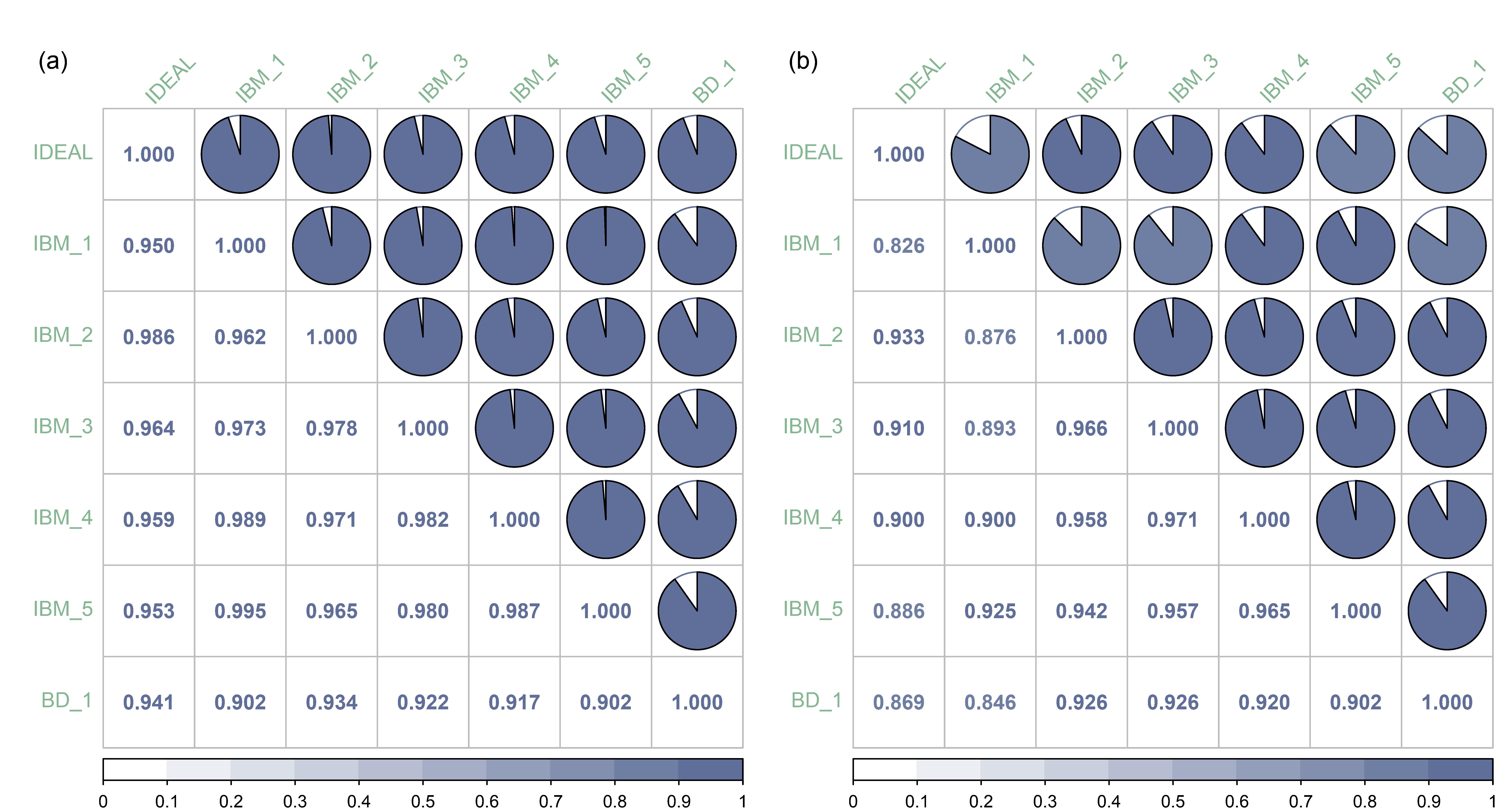
Figure 2: The performance matrices for the single-qubit H and two-qubit CNOT gates generated from seven different quantum platforms. The entry in the $i$-th row and $j$-th column of the matrix represents the max process fidelity between platform-$i$ and platform-$j$. The entries in the upper right corner are visualized in pie chart format. (a) The performance matrix of the H gate. Each entry is inferred from $2^{1}\cdot N_{U}=20$ random circuits and each circuit is repeated $M_{\rm shots}=500$ times. (b) The performance matrix of the CNOT gate. Each entry is inferred from $2^{2}\cdot N_{U}=20$ random circuits and each circuit is repeated $M_{\rm shots}=500$ times.

III.4 Comparison with previous works

Knörzer et al. [18] have recently introduced a new set of protocols that enable pair-wise comparisons between distant nodes in a quantum network. The authors propose four cross-platform state comparison schemes as alternatives to Elben’s protocol [17], each of which relies on the presence of quantum links. In addition to this, they present three protocols, referred to as M1, M2, and M3, which facilitate cross-platform comparisons of quantum processes, assuming that a cross-platform state comparison protocol is available.

We will now explain how our protocol differs from M1, M2, and M3. While M1 involves an ancilla-assisted comparison protocol that we have rephrased in Section III.1, our protocol does not rely on ancilla qubits. Similarly, M3 involves a series of entanglement tests that are fundamentally different from our protocol. Although our protocol and M2 share some similarities, such as the absence of ancilla qubits and the need to sample random unitaries and computational basis states, there are notable differences. Specifically, our protocol only needs to sample from a single-qubit unitary $2$-design, can accurately estimate the max fidelity, and can compare the performance of arbitrary quantum processes. On the other hand, M2(i) estimates the average gate fidelity and requires sampling from a multi-qubit unitary $2$-design, which can be resource-intensive as the number of qubits increases. M2(iii) is conceptually straightforward but can only estimate the ability of quantum processes to preserve quantum information in the computational basis. Additionally, M2(i) and M2(iii) are limited to comparing the performance of unitary quantum processes.

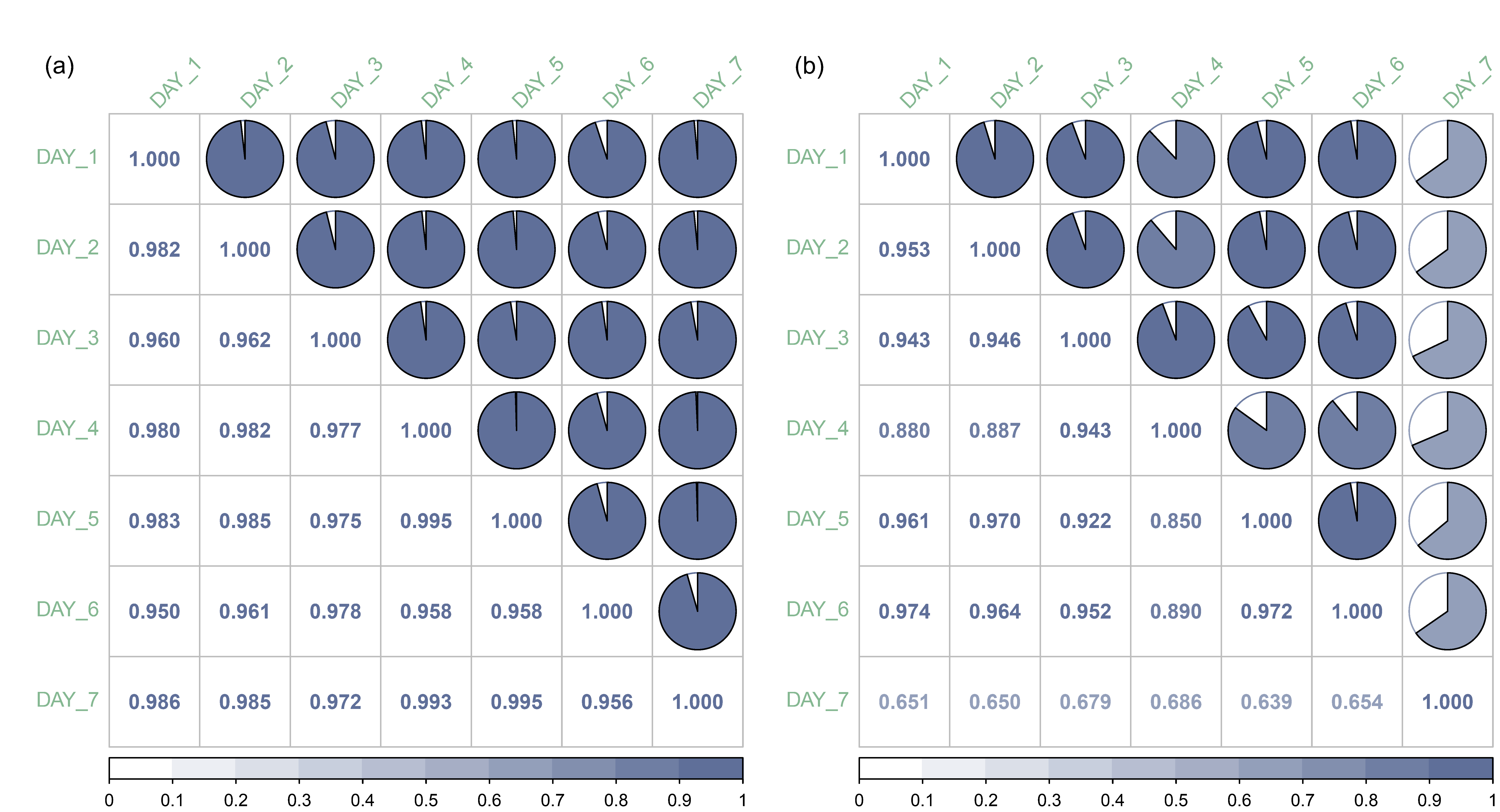
Figure 3: The performance matrices of the single-qubit H and two-qubit CNOT gates generated from the daily data of Baidu’s "Qianshi" quantum computer for one week. The entry in the $i$-th row and $j$-th column of the matrix represents the max process fidelity between platform-$i$ and platform-$j$. The entries in the upper right corner are visualized in pie chart format. (a) The performance matrix of the H gate. Each entry is inferred from $2^{1}\cdot N_{U}=20$ random circuits and each circuit is repeated $M_{\rm shots}=500$ times. (b) The performance matrix of the CNOT gate. Each entry is inferred from $2^{2}\cdot N_{U}=400$ random circuits and each circuit is repeated $M_{\rm shots}=500$ times.

IV Experiments

In this section, we report experimental results on cross-platform comparison of quantum processes across various spatially and temporally separated quantum devices. First, we demonstrate the efficacy of our protocol in comparing the H and CNOT gates implemented on different platforms with their ideal counterparts obtained from classical simulation. Next, we monitor the stability of the "Qianshi" quantum computer from Baidu over a week with our protocol. Finally, we conduct an extensive numerical analysis to determine the expected number of experimental runs required to obtain reliable results. All the experiments are conducted using the Quantum Error Processing toolkit developed on the Baidu Quantum Platform [31].

IV.1 Comparing spatially separated quantum processes

We utilize our ancilla-free cross-platform comparison protocol to assess the performance of H and CNOT gates implemented on seven distinct platforms that are freely accessible to the public over the internet. These platforms include six superconducting quantum computers, namely ibmq_quito (IBM_1), ibmq_oslo (IBM_2), ibmq_lima (IBM_3), ibm_nairobi (IBM_4), ibmq_manila (IBM_5), and baidu_qianshi (BD_1), as well as the baidu ideal simulator (IDEAL), which is intended for experiment-theory comparisons.

First of all, it is noteworthy that the random Pauli basis measurements $\{X,Y,Z\}$ are equivalent to randomized measurements with a single qubit Clifford group [24, 32]. The Clifford group is a unitary $2$-design group, and it can be employed to conduct complete process tomography of $n$-qubit quantum processes. This equivalence enables us to sample directly from the $3^{n}$ Pauli preparation and $3^{n}$ Pauli measurement unitaries in our experiments.

To begin with, we utilize our protocol to compare the performance of the single-qubit H gate across seven quantum platforms. To achieve this, we create $2^{1}\times N_{U}=20$ random circuits and execute $M_{\rm shots}=500$ projective measurements for each circuit on each platform. Furthermore, we employ the same protocol to compare the performance of the CNOT gate implemented on these platforms. To accomplish this, we generate $2^{2}\times N_{U}=400$ random circuits and performe $M_{\rm shots}=500$ repetitions for each quantum circuit on each platform. The performance matrices for the H and CNOT gates are presented in Figure 2.

The experimental results make it clear that, while some quantum devices may achieve fidelities that are comparable to those of the ideal simulator, there remains a significant discrepancy between them. This emphasizes the importance of directly comparing the performance of quantum devices with each other, rather than relying solely on comparisons to an ideal simulator, as such comparisons may not be adequate.

IV.2 Comparing temporally separated quantum processes

Our protocol is also useful for monitoring the stable performance of quantum devices. To this end, we employe the ancilla-free cross-platform comparison protocol to assess the stability of H and CNOT gates implemented on Baidu’s "Qianshi" quantum computer (BD_1) over the course of one week. The experimental settings for the H and CNOT gates are identical to those used in the previous section. Specifically, for the single-qubit H gate, we create $2^{1}\times N_{U}=20$ random circuits daily and execute $M_{\rm shots}=500$ projective measurements for each circuit on "Qianshi". For the two-qubit CNOT gate, we create $2^{2}\times N_{U}=400$ random circuits daily and execute $M_{\rm shots}=500$ projective measurements for each circuit on "Qianshi". The performance matrices of the single-qubit H and two-qubit CNOT gates generated from the daily data of "Qianshi" are shown in Figure 3.

After analyzing the cross-platform fidelities presented in Figure 3, we discover several noteworthy features. First, we observe that the stability of the H gate is considerably higher than that of the CNOT gate on "Qianshi," which aligns with the expectation that two-qubit gates are harder to implement and maintain in a superconducting quantum computer than single-qubit gates. Additionally, on the last day of the week (DAY_7), there is a significant drop in the performance of the CNOT gate. After consulting with researchers from Baidu’s Quantum Computing Hardware Laboratory, it is determined that the instability is caused by the sudden halt of the dilution cooling system. After the system is restarted, all native quantum gates have to be re-calibrated to achieve optimal performance. Furthermore, it is observed that the temperature variation had a negligible impact on the H gate. This observation might be helpful for the experimenters to identify potential hardware issues.

IV.3 Scaling of the required number of experimental runs

Figure 4: Average statistical error $|\widetilde{F}_{\max}-1|$ as a function of the total number of experimental runs $2^{n}N_{U}M_{\rm shots}$. The target quantum process is taken to be the H gate for $n=1$ and the CNOT gate for $n=2$. The green lines obey $\sim 1/(2^{n}N_{U}M_{\rm shots})$ and are guides for the eye. The data is obtained via numerical simulation.

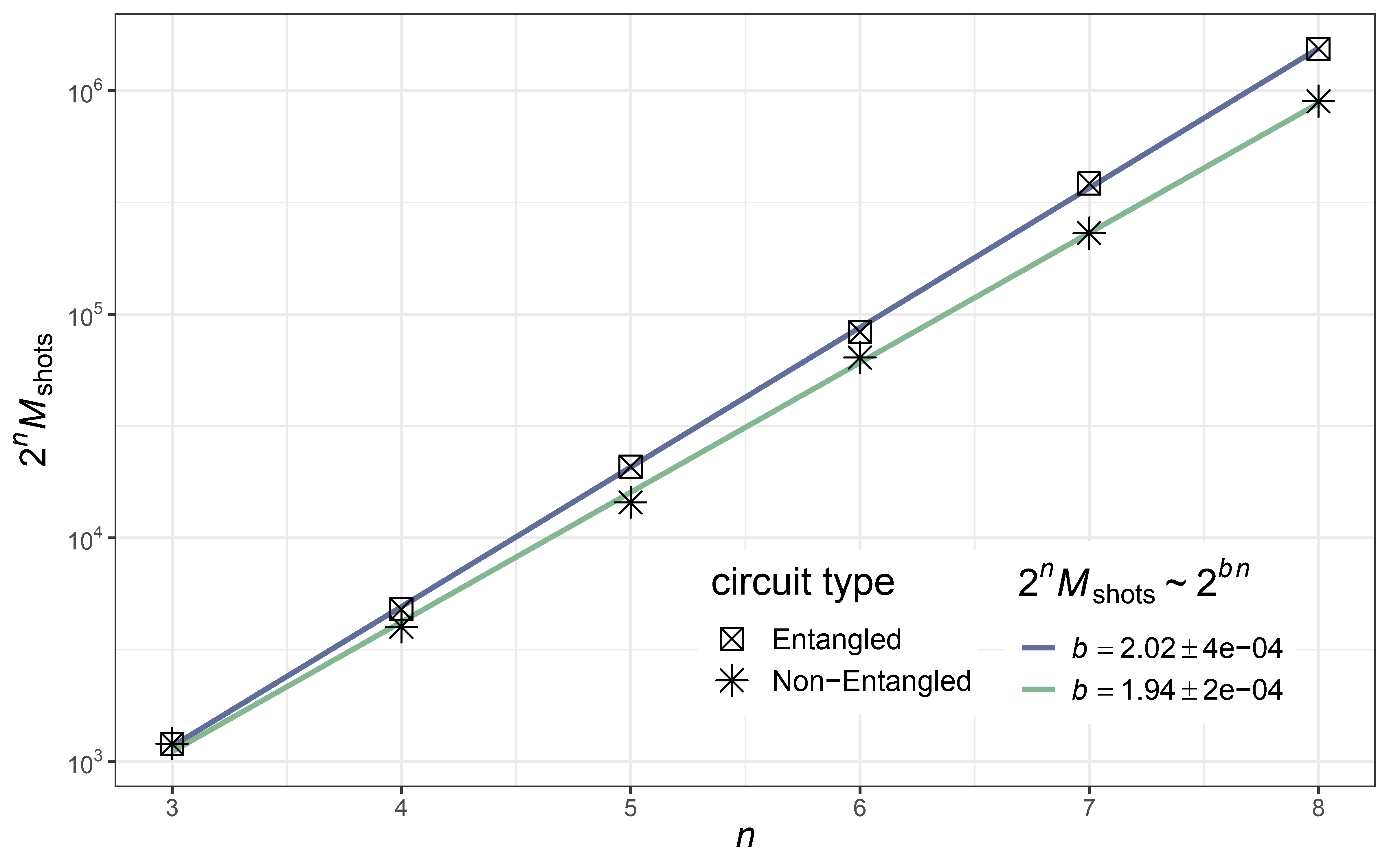
Figure 5: Scaling of the minimal number of required experimental runs $2^{n}M_{\rm shots}$ to estimate $\widetilde{F}_{\max}$ up to a fixed statistical error of $0.05$ as a function of the number of qubits $n$. The number of random unitaries is fixed to $N_{U}=100$. The target quantum process is taken to be the $n$-qubit GHZ state preparation circuit for the entangled case and the rotation circuit composed of $n$ single-qubit rotation gates for the non-entangled case. The data is obtained via numerical simulation.

In practice, the accuracy of the estimated fidelity is unavoidably subject to statistical error, as a result of the finite number of random circuits ($2^{n}\cdot N_{U}$) and the finite number of projective measurements ($M_{\rm shots}$) performed per random circuit. Therefore, it is experimentally crucial to consider the scaling of the total number of experimental runs, which equals to $2^{n}\cdot N_{U}\cdot M_{\rm shots}$, constituting the measurement budget, in order to effectively suppress the statistical error to a prespecified threshold $\epsilon$ when evaluating the performance of an $n$-qubit quantum process. In the following, we present numerical simulation to investigate this behavior.

In Figure 4, numerical results for the average statistical error as a function of the measurement budget $2^{n}\cdot N_{U}\cdot M_{\rm shots}$ are presented and the scaling of the measurement budget with respect to the system size $n$ is derived. In order to keep consistent with previous experiments, we choose the H gate when $n=1$ and the CNOT gate when $n=2$ in the simulation. Note that in this case the ideal fidelity $F_{\max}=1$ is known. We repeat our protocol on the ideal simulator $5$ times for each point in the figure and record the mean of the statistical errors $|\widetilde{F}_{\max}-1.0|$. We find that the statistical error scales as $|\widetilde{F}_{\max}-1.0|\sim 1/(2^{n}N_{U}M_{\rm shots})$, where $\widetilde{F}_{\max}$ is the estimated max process fidelity via simulation.

Now we investigate the scaling of the required number of experimental runs, $2^{n}M_{\rm shots}$, per unitary to estimate the max fidelity $\widetilde{F}_{\max}$ within an average statistical error of $\epsilon=0.05$ while fixing $N_{U}$ to $100$. We employ our protocol to two very different types of quantum processes, with different numbers of qubits $n$: (i) a highly entangled quantum process corresponding to an $n$-qubit GHZ state preparation circuit (Entangled) and (ii) a completely local quantum process composed of $n$ single-qubit rotation gates (Non-Entangled). The numerical results are presented in Figure 5. From the fitted data, we find that $2^{n}M_{\rm shots}\sim 2^{bn}$, where $b=2.02\pm 4{\rm e-}4$ for the entangled case and $b=1.94\pm 2{\rm e-}4$ for the non-entangled case. The analysis shows that our ancilla-free cross-platform protocol requires a total number of experimental runs that scales as $2^{n}N_{U}M_{\rm shots}\sim 2^{bn}$ with $b\approx 2$. This scaling, despite exponential, is significantly less than full quantum process tomography (QPT), which has an exponent $b\geq 4$ [33].

V Conclusions

We have proposed an ancilla-free cross-platform protocol that enables the performance comparison of arbitrary quantum processes, using only single-qubit unitaries and classical communication. This protocol is thus suitable for comparing quantum processes that are independently manufactured over different times and locations, built by different teams using different technologies. We have experimentally demonstrated the cross-platform protocol on six remote quantum computers fabricated by IBM and Baidu, and monitored the stable functioning of Baidu’s "Qianshi" quantum computer over one week. The experimental results reveal that our protocol accurately compares the performance of different quantum computers with significantly fewer measurements than quantum process tomography. Additionally, we have shown that our protocol is applicable to quantum process tomography.

However, some problems must be further explored to make the cross-platform protocols more practical. Firstly, the sample complexity of these protocols lacks theoretical guarantees, thereby necessitating the empirical selection of experimental parameters. To address this challenge, it may be possible to adapt techniques from [34]. Secondly, it is vital to make the protocols robust against state preparation and measurement errors. One possible solution is to apply quantum error mitigation methods [35, 36, 37, 38, 39] to alleviate quantum errors and increase the estimation accuracy. We suggest that ideas and insights from randomized benchmarking [40] and quantum gateset tomography [41] might be helpful for designing error robust cross-platform protocols.

Appendix A Proof of the protocol

In this section, we prove the correctness of the ancilla-free cross-platform comparison protocol introduced in the main text (MT).

For two $n$-qubit quantum processes $\mathcal{E}_{1}$ and $\mathcal{E}_{2}$ performed on platforms $\mathcal{S}_{1}$ and $\mathcal{S}_{2}$, let’s start with the ancilla-assisted idea for estimating $\operatorname{Tr}[\eta_{i}\eta_{j}]$. On each platform, we prepare a $2n$-qubit maximally entangled state with an $n$-qubit auxiliary system and apply the corresponding quantum process $\mathcal{E}_{i}$ to the target quantum system. This enables us to construct the Choi state $\eta_{i}$ of the quantum process $\mathcal{E}_{i}$. Using Eq. (2) in MT, we can estimate the overlap between the Choi states $\eta_{i}$ and $\eta_{j}$, where $i,j=1,2$, via

$$\operatorname{Tr}[\eta_{i}\eta_{j}]=4^{n}\sum_{\bm{s},\bm{s}^{\prime},\bm{k},\bm{k}^{\prime}\in\{0,1\}^{n}}(-2)^{-\mathcal{D}[\bm{s},\bm{s}^{\prime}]-\mathcal{D}[\bm{k},\bm{k}^{\prime}]}\overline{{\rm Pr}_{U}^{(i)}[\bm{s},\bm{k}]{\rm Pr}_{U}^{(j)}[\bm{s}^{\prime},\bm{k}^{\prime}]},$$ (7)

where $\bm{s}$ and $\bm{k}$ are bitstrings representing the outcomes of the auxiliary system and the original system, respectively. $\overline{\cdots}$ denotes ensemble average over $U$, where $U$ is a tensor product of $2n$ local random unitaries sampled from a single-qubit set $\mathcal{X}_{2}$ satisfying unitary $2$-design.

The key trick for removing the ancilla qubits from (7) is that we can generate the probability distribution ${\rm Pr}_{U}^{(i)}[\bm{s},\bm{k}]$ through a prepare-and-measure approach, without requiring the use of any ancilla qubits. Since $U$ is a tensor product of $2n$ local random unitaries, we can decompose it as $U=U_{1}\otimes U_{2}$, where $U_{1}$ and $U_{2}$ are the unitaries operating on the auxiliary and original systems, respectively. Note that both $U_{1}$ and $U_{2}$ are tensor products of $n$ local random unitaries. Based on this decomposition, we can rewrite the probability distribution ${\rm Pr}_{U}^{(i)}[\bm{s},\bm{k}]$ in Eq. (7) as

$${\rm Pr}_{U}^{(i)}[\bm{s},\bm{k}] =\operatorname{Tr}\left[(|{\bm{s}\bm{k}}\rangle\!\langle{\bm{s}\bm{k}}|)\left(U\eta_{i}U^{\dagger}\right)\right]$$ (8)

$$=\operatorname{Tr}\left\{(|{\bm{s}\bm{k}}\rangle\!\langle{\bm{s}\bm{k}}|)\left[(U_{1}\otimes U_{2})(\mathcal{I}\otimes\mathcal{E}_{i})(|{\psi_{+}}\rangle\!\langle{\psi_{+}}|)(U_{1}\otimes U_{2})^{\dagger}\right]\right\}$$ (9)

$$=\operatorname{Tr}\left\{\left[(U_{1}^{\dagger}|{\bm{s}}\rangle\!\langle{\bm{s}}|U_{1})\otimes\left((|{\bm{k}}\rangle\!\langle{\bm{k}}|)(\mathcal{U}_{2}\circ\mathcal{E}_{i})\right)\right](|{\psi_{+}}\rangle\!\langle{\psi_{+}}|)\right\}$$ (10)

$$=\operatorname{Tr}\left\{(U_{1}^{\dagger}|{\bm{s}}\rangle\!\langle{\bm{s}}|U_{1})\otimes|{\bm{k}}\rangle\!\langle{\bm{k}}|(\mathcal{U}_{2}\circ\mathcal{E}_{i})(U_{1}^{T}|{\bm{s}}\rangle\!\langle{\bm{s}}|U_{1}^{*})\right\}$$ (11)

$$=\operatorname{Tr}\left[|{\bm{k}}\rangle\!\langle{\bm{k}}|(\mathcal{U}_{2}\circ\mathcal{E}_{i})(U_{1}^{T}|{\bm{s}}\rangle\!\langle{\bm{s}}|U_{1}^{*})\right],$$ (12)

where $\mathcal{U}_{i}(\cdot)=U_{i}(\cdot)U_{i}^{\dagger}$ and Eq. (11) follows from the identity $(|{u}\rangle\!\langle{u}|\otimes\mathbbm{1})\left|{\psi_{+}}\right\rangle=\left|{u}\right\rangle\otimes\left|{u^{*}}\right\rangle$. Eq. (12) leads to an ancilla-free approach to generate the probability distribution ${\rm Pr}_{U}^{(i)}[\bm{s},\bm{k}]$ as follows: We prepare the input state $U_{1}^{T}\left|{\bm{s}}\right\rangle$, execute the target quantum process $\mathcal{E}_{i}$, followed by the unitary $U_{2}$, and measure the resulting state in the computational basis. The remaining question is what probability distribution should be used to sample and prepare the computational basis input states $\left|{\bm{s}}\right\rangle$. Since the reduced state of a maximally entangled state is the maximally mixed state, we conclude that the measurement outcomes of the auxiliary system satisfy the uniform distribution for arbitrary randomized measurements, i.e.,

$$\Pr\left\{S=\bm{s}|U_{1}\right\}=\frac{1}{2^{n}}.$$ (13)

That is, the computational basis input states $\left|{\bm{s}}\right\rangle$ should be sampled and prepared with respect to the uniform distribution. This accomplishes the final piece of the ancilla-free cross-platform estimation protocol.

Appendix B Randomized quantum process tomography

In this section, we prove the correctness of randomized quantum process tomography in the MT.

In [30], it was shown that the full information of an $n$-qubit unknown quantum state $\rho$ can be reconstructed using the experimental data $\{\Pr_{U}^{(1)},\Pr_{U}^{(2)}\}_{U}$ collected in Section II.1 via

$$\rho_{i}=2^{n}\sum_{\bm{s},\bm{s}^{\prime}\in\{0,1\}^{n}}(-2)^{-\mathcal{D}[\bm{s},\bm{s}^{\prime}]}\overline{{\rm Pr}_{U}^{(i)}[\bm{s}]U^{\dagger}|{\bm{s}^{\prime}}\rangle\!\langle{\bm{s}^{\prime}}|U},$$ (14)

where $i=1,2$ and $\overline{\cdots}$ denotes ensemble averaging over $U$, which is a tensor product of $n$ local random unitaries sampled from $\mathcal{X}_{2}$.

Similarly, we can adopt the experimental data collected by cross-platform process comparison protocols to reconstruct the full information of an unknown quantum process. Let’s begin with the ancilla-assisted protocol for reconstructing an $n$-qubit quantum process $\mathcal{E}_{i}$, $i=1,2$. We prepare a $2n$-qubit maximally entangled state with an $n$-qubit auxiliary system. Then the randomized measurement protocol outlined in (14) provides a simple way to reconstruct the Choi state of the quantum process $\mathcal{E}$ via

$$\eta_{\mathcal{E}_{i}}=4^{n}\sum_{\bm{s},\bm{s}^{\prime},\bm{k},\bm{k}^{\prime}\in\{0,1\}^{n}}(-2)^{-\mathcal{D}[\bm{s},\bm{s}^{\prime}]-\mathcal{D}[\bm{k},\bm{k}^{\prime}]}\overline{{\rm Pr}_{U}^{(i)}[\bm{s},\bm{k}]U^{\dagger}|{\bm{s}^{\prime}\bm{k}^{\prime}}\rangle\!\langle{\bm{s}^{\prime}\bm{k}^{\prime}}|U},$$ (15)

using the experimental data ${\rm Pr}_{U}^{(i)}[\bm{s},\bm{k}]$ collected in Section III.1. Note that here $\overline{\cdots}$ denotes ensemble averaging over $U$, which is a tensor product of $2n$ local random unitaries sampled from $\mathcal{X}_{2}$.

As proved in Appendix A, the probability distribution ${\rm Pr}_{U}^{(i)}[\bm{s},\bm{k}]$ can be generated using a prepare-and-measure approach that does not require the use of ancilla qubits. Specifically, we decompose each $U$ as $U=U_{1}\otimes U_{2}$, where $U_{1}^{T}$ and $U_{2}$ are employed for state preparation and randomized measurement, respectively. The ancilla-free approach reconstructs the Choi state of the quantum process $\mathcal{E}$ with the same formula as Eq. (15). The advantage is that it facilitates the reconstruction in a more practical manner.

References

- Preskill [2018] J. Preskill, Quantum computing in the NISQ era and beyond, Quantum 2, 79 (2018).
- O’Donnell and Wright [2016] R. O’Donnell and J. Wright, Efficient quantum tomography, in Proceedings of the Forty-Eighth Annual ACM Symposium on Theory of Computing (2016) pp. 899–912.
- Häffner et al. [2005] H. Häffner, W. Hänsel, C. Roos, J. Benhelm, D. Chek-al Kar, M. Chwalla, T. Körber, U. Rapol, M. Riebe, P. Schmidt, et al., Scalable multiparticle entanglement of trapped ions, Nature 438, 643 (2005).
- Carolan et al. [2014] J. Carolan, J. D. Meinecke, P. J. Shadbolt, N. J. Russell, N. Ismail, K. Wörhoff, T. Rudolph, M. G. Thompson, J. L. O’brien, J. C. Matthews, et al., On the experimental verification of quantum complexity in linear optics, Nature Photonics 8, 621 (2014).
- Eisert et al. [2020] J. Eisert, D. Hangleiter, N. Walk, I. Roth, D. Markham, R. Parekh, U. Chabaud, and E. Kashefi, Quantum certification and benchmarking, Nature Reviews Physics 2, 382 (2020).
- Kliesch and Roth [2021] M. Kliesch and I. Roth, Theory of quantum system certification, PRX quantum 2, 010201 (2021).
- Hofmann [2005] H. F. Hofmann, Complementary classical fidelities as an efficient criterion for the evaluation of experimentally realized quantum operations, Physical Review Letters 94, 160504 (2005).
- Bendersky et al. [2008] A. Bendersky, F. Pastawski, and J. P. Paz, Selective and efficient estimation of parameters for quantum process tomography, Physical Review Letters 100, 190403 (2008).
- Flammia and Liu [2011] S. T. Flammia and Y.-K. Liu, Direct fidelity estimation from few pauli measurements, Physical Review Letters 106, 230501 (2011).
- da Silva et al. [2011] M. P. da Silva, O. Landon-Cardinal, and D. Poulin, Practical characterization of quantum devices without tomography, Physical Review Letters 107, 210404 (2011).
- Reich et al. [2013] D. M. Reich, G. Gualdi, and C. P. Koch, Optimal strategies for estimating the average fidelity of quantum gates, Physical Review Letters 111, 200401 (2013).
- Greenaway et al. [2021] S. Greenaway, F. Sauvage, K. E. Khosla, and F. Mintert, Efficient assessment of process fidelity, Physical Review Research 3, 033031 (2021).
- Pallister et al. [2018] S. Pallister, N. Linden, and A. Montanaro, Optimal verification of entangled states with local measurements, Physical Review Letters 120, 170502 (2018).
- Zhu and Hayashi [2019] H. Zhu and M. Hayashi, Efficient verification of pure quantum states in the adversarial scenario, Physical Review Letters 123, 260504 (2019).
- Wang and Hayashi [2019] K. Wang and M. Hayashi, Optimal verification of two-qubit pure states, Phys. Rev. A 100, 032315 (2019).
- Yu et al. [2022] X.-D. Yu, J. Shang, and O. Gühne, Statistical methods for quantum state verification and fidelity estimation, Advanced Quantum Technologies 5, 2100126 (2022).
- Elben et al. [2020] A. Elben, B. Vermersch, R. van Bijnen, C. Kokail, T. Brydges, C. Maier, M. K. Joshi, R. Blatt, C. F. Roos, and P. Zoller, Cross-platform verification of intermediate scale quantum devices, Physical Review Letters 124, 010504 (2020).
- Knörzer et al. [2022] J. Knörzer, D. Malz, and J. I. Cirac, Cross-platform verification in quantum networks, arXiv preprint arXiv:2212.07789 10.48550/arXiv.2212.07789 (2022).
- Elben et al. [2022] A. Elben, S. T. Flammia, H.-Y. Huang, R. Kueng, J. Preskill, B. Vermersch, and P. Zoller, The randomized measurement toolbox, Nature Reviews Physics 5, 9 (2022).
- Liang et al. [2019] Y.-C. Liang, Y.-H. Yeh, P. E. Mendonça, R. Y. Teh, M. D. Reid, and P. D. Drummond, Quantum fidelity measures for mixed states, Reports on Progress in Physics 82, 076001 (2019).
- Dankert et al. [2009] C. Dankert, R. Cleve, J. Emerson, and E. Livine, Exact and approximate unitary 2-designs and their application to fidelity estimation, Physical Review A 80, 012304 (2009).
- Gross et al. [2007] D. Gross, K. Audenaert, and J. Eisert, Evenly distributed unitaries: On the structure of unitary designs, Journal of Mathematical Physics 48, 052104 (2007).
- Brydges et al. [2019] T. Brydges, A. Elben, P. Jurcevic, B. Vermersch, C. Maier, B. P. Lanyon, P. Zoller, R. Blatt, and C. F. Roos, Probing rényi entanglement entropy via randomized measurements, Science 364, 260 (2019).
- Zhu et al. [2022] D. Zhu, Z.-P. Cian, C. Noel, A. Risinger, D. Biswas, L. Egan, Y. Zhu, A. M. Green, C. H. Alderete, N. H. Nguyen, et al., Cross-platform comparison of arbitrary quantum states, Nature Communications 13, 6620 (2022).
- Watrous [2018] J. Watrous, The Theory of Quantum Information (Cambridge University Press, 2018).
- Jamiołkowski [1972] A. Jamiołkowski, Linear transformations which preserve trace and positive semidefiniteness of operators, Reports on Mathematical Physics 3, 275 (1972).
- Gilchrist et al. [2005] A. Gilchrist, N. K. Langford, and M. A. Nielsen, Distance measures to compare real and ideal quantum processes, Physical Review A 71, 062310 (2005).
- Nielsen and Chuang [2010] M. A. Nielsen and I. L. Chuang, Quantum Computation and Quantum Information: 10th Anniversary Edition (Cambridge University Press, 2010).
- Korzekwa et al. [2018] K. Korzekwa, S. Czachórski, Z. Puchała, and K. Życzkowski, Coherifying quantum channels, New Journal of Physics 20, 043028 (2018).
- Elben et al. [2019] A. Elben, B. Vermersch, C. F. Roos, and P. Zoller, Statistical correlations between locally randomized measurements: A toolbox for probing entanglement in many-body quantum states, Physical Review A 99, 052323 (2019).
- Baidu Quantum [2022] Baidu Quantum, Quantum Error Processing Toolkit (QEP) (2022).
- Huang et al. [2020] H.-Y. Huang, R. Kueng, and J. Preskill, Predicting many properties of a quantum system from very few measurements, Nature Physics 16, 1050 (2020).
- Mohseni et al. [2008] M. Mohseni, A. T. Rezakhani, and D. A. Lidar, Quantum-process tomography: Resource analysis of different strategies, Physical Review A 77, 032322 (2008).
- Anshu et al. [2022] A. Anshu, Z. Landau, and Y. Liu, Distributed quantum inner product estimation, in Proceedings of the 54th Annual ACM SIGACT Symposium on Theory of Computing (ACM, 2022).
- Temme et al. [2017] K. Temme, S. Bravyi, and J. M. Gambetta, Error mitigation for short-depth quantum circuits, Physical Review Letters 119, 180509 (2017).
- Kandala et al. [2019] A. Kandala, K. Temme, A. D. Córcoles, A. Mezzacapo, J. M. Chow, and J. M. Gambetta, Error mitigation extends the computational reach of a noisy quantum processor, Nature 567, 491 (2019).
- Wang et al. [2021] K. Wang, Y.-A. Chen, and X. Wang, Mitigating Quantum Errors via Truncated Neumann Series, arXiv preprint arXiv:2111.00691 10.48550/arXiv.2111.00691 (2021).
- Tang et al. [2022] S. Tang, C. Zheng, and K. Wang, Detecting and Eliminating Quantum Noise of Quantum Measurements, arXiv preprint arXiv:2206.13743 10.48550/arXiv.2206.13743 (2022).
- Cai et al. [2022] Z. Cai, R. Babbush, S. C. Benjamin, S. Endo, W. J. Huggins, Y. Li, J. R. McClean, and T. E. O’Brien, Quantum error mitigation, arXiv preprint arXiv:2210.00921 10.48550/arXiv.2210.00921 (2022).
- Helsen et al. [2022] J. Helsen, I. Roth, E. Onorati, A. Werner, and J. Eisert, General framework for randomized benchmarking, PRX Quantum 3, 020357 (2022).
- Nielsen et al. [2021] E. Nielsen, J. K. Gamble, K. Rudinger, T. Scholten, K. Young, and R. Blume-Kohout, Gate Set Tomography, Quantum 5, 557 (2021).