Regularization of polynomial networks for image recognition

Abstract

Deep Neural Networks (DNNs) have obtained impressive performance across tasks, however they still remain as black boxes, e.g., hard to theoretically analyze. At the same time, Polynomial Networks (PNs) have emerged as an alternative method with a promising performance and improved interpretability but have yet to reach the performance of the powerful DNN baselines. In this work, we aim to close this performance gap. We introduce a class of PNs, which are able to reach the performance of ResNet across a range of six benchmarks. We demonstrate that strong regularization is critical and conduct an extensive study of the exact regularization schemes required to match performance. To further motivate the regularization schemes, we introduce $\mathcal{D}$-PolyNets that achieve a higher-degree of expansion than previously proposed polynomial networks. $\mathcal{D}$-PolyNets are more parameter-efficient while achieving a similar performance as other polynomial networks. We expect that our new models can lead to an understanding of the role of elementwise activation functions (which are no longer required for training PNs). The source code is available at https://github.com/grigorisg9gr/regularized_polynomials.

1 Introduction

Deep neural networks (DNNs) are dominating the research agenda in computer vision since the previous decade owing to their stellar performance in image recognition [24, 17] and object detection [28, 27]. The design of tailored normalization schemes [21], data augmentation [11] and specific architectural blocks [19, 42] have further fostered this trend. However, our theoretical understanding of DNNs pales in comparison. There is little progress in making DNNs interpretable, or a principled understanding of the training dynamics or the role of the network depth.

Figure 1: The proposed networks ($\mathcal{R}$-PolyNets, $\mathcal{D}$-PolyNets) enable polynomial networks to reach the performance of the powerful neural networks across a range of tasks.

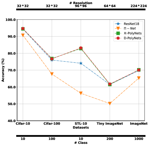
So far, a handful of works have attempted to mitigate that lack of understanding by designing principled architectures. Combining neural networks with the research on kernel methods has emerged for designing principled architectures with guarantees. In [30], the kernel feature map of the training data is used for achieving invariance to certain transformations. Recently, high-performing kernels were used for defining a principled architecture [40]. Using fixed components such as wavelets has been considered for replacing the learnable convolutions [33]. Another approach approximates the target function with a polynomial expansion. Polynomial Nets (PNs) rely on capturing higher-order correlations of the input data for expressing the output without the use of elementwise activation functions [37]. Despite the progress in the principled design of networks, the aforementioned works have yet to achieve a performance comparable to standard baselines, such as the performance of the seminal residual neural networks (ResNet) [17].

In this work, we aim to close the gap between well-established neural network architectures and principled architectures by focusing on the PNs. In particular, we concentrate on the recent parametrization of $\Pi$-Nets [5] that has outperformed the aforementioned principled methods. We validate our hypothesis that the performance of PNs can be significantly improved through strong regularization schemes. To this end, we introduce a class of polynomial networks, called $\mathcal{R}$-PolyNets. In our study, we explore which regularization schemes can improve the performance of PNs. For instance, we find that initializations proposed for neural networks [15, 36] are not optimal for PNs. Overall, our exploration enables $\mathcal{R}$-PolyNets to achieve performance on par with the (unregularized) ResNet, which is the de facto neural network baseline.

To further motivate our regularization schemes, we design a new class of polynomial expansions achieving a higher total degree of expansion than previous PNs. In $\mathcal{R}$-PolyNets, the final degree of expansion is obtained by a sequential concatenation of a series of lower-degree polynomial expansions. That is, $\mathcal{R}$-PolyNets concatenate $N$ polynomials of second-degree to obtain a $2^{N}$ polynomial expansion. Instead, we use outputs from previous polynomials in the current expansion, increasing the previous total degree. Our goals are twofold: a) transfer representations from earlier polynomials, b) increase the total degree of polynomial expansion. The proposed regularization schemes are critical for training these dense polynomials, named $\mathcal{D}$-PolyNets. We showcase that $\mathcal{D}$-PolyNets are more expressive than previously proposed polynomial expansions. Overall, our contributions can be summarized as follows:

• We introduce a class of regularized polynomial networks, called $\mathcal{R}$-PolyNets, in sec. 3.

• We propose densely connected polynomials, called $\mathcal{D}$-PolyNets. $\mathcal{D}$-PolyNets use multiple terms from a previous polynomial as input to the current polynomial resulting in a higher-degree of expansion than previous PNs (sec. 4).

• Our thorough validation in both image and audio recognition illustrates the critical components for achieving performance equivalent to vanilla DNNs.

2 Related work

2.1 Polynomial networks

Polynomial networks (PNs) capture higher-order interactions between the input elements using high-degree polynomial expansions. PNs have demonstrated a promising performance in standard benchmarks in image generation [5] and image recognition [4]. Beyond the empirical progress, various (theoretical) properties of PNs have been recently explored [53, 34]. In particular, PNs augment the expressivity of DNNs [13], while they offer benefits in the extrapolation or learning high-frequency functions [3, 47]. More importantly, the recent work of [12] highlights how PNs can learn powerful interpretable models.

When PNs are combined with element-wise activation functions, they can achieve state-of-the-art performance as demonstrated in [44, 18, 26, 5, 1, 50, 49]. However, many of the beneficial properties, such as the interpretability are not applicable for these models. Therefore, the hybrid models combining polynomial expansions with activation functions are not the focus of our work, since they share similar drawbacks to DNNs.

Table 1: Nomenclature on the symbols used in this work

Symbol	Dimension(s)	Definition
$n,N$	$\mathbb{N}$	Polynomial term degree, total approximation degree.
$r$	$\mathbb{N}$	Rank of the decomposition.
$\bm{z}$	$\mathbb{R}^{d}$	Input to polynomial expansion.
$\bm{B},\theta$	$\mathbb{R}^{o\times r},\mathbb{R}^{o}$	Parameters in the decomposition.
$\bm{H}_{[n]},\bm{J}_{[n]},\bm{K}_{[n]}$	$\mathbb{R}^{d\times r},\mathbb{R}^{k\times r},\mathbb{R}^{\omega\times r}$	Parameters in the hierarchical decomposition.
$\bm{\Phi},\bm{\Psi}$	$\mathbb{R}^{r\times r},\mathbb{R}^{r\times r}$	Regularization matrices.
$*$	$-$	Hadamard (element-wise) product.

2.2 Regularization of neural networks

Deep neural networks (DNNs) can be prone to over-fitting and regularization methods are widely used to mitigate this issue. Hence, we summarize below three categories of regularization techniques: a) data augmentation, b) intermediate learned features and c) auxiliary loss terms.

Data augmentation: Data augmentation techniques are often used in image recognition pipelines [52, 11, 51]. Mixup [52] uses a linear interpolation between two training samples to improve generalization based on empirical vicinal risk minimization [2]. Cutout [11] removes contiguous regions from the input images, generating augmented training dataset with partially occluded versions of existing samples. This enables the network to focus on non-dominant part of the training sample. CutMix [51] combines the previous two augmentation methods by replacing a patch of the image with a patch from another training image.

Feature normalization: Apart from the data augmentation, feature normalization enables deeper neural networks to be trained. Dropout [41] is a prominent example of such feature normalization techniques. Dropout randomly drops units (and the corresponding connections) during training to avoid co-adaptation of units. Despite its initial success, dropout has not been widely used with convolutional neural nets. Instead, dropblock [14] randomly drops a contiguous region of a feature map. Additional regularization schemes, such as average or max pooling, rely on the idea of aggregating features from a local region of the feature map to avoid the sensitivity to small spatial distortions [6].

Auxiliary loss terms: In addition to the classification losses, additional loss terms, such as Tikhonov regularization, can result in more stable learning and can avoid overfitting [39] [Chapter 13]. Weight decay forces sparsity on the weights by penalizing their norm. [8] proposes to decorrelate the different units by encouraging the covariance matrix of the features to be close to the identity matrix. For classification problems, label smoothing can prevent the networks from predicting the training examples over-confidently [31].

Despite the progress in regularization schemes and the various theoretical connections, no consensus has been reached over a single regularization scheme that performs well in all cases, so often a combination of regularization schemes are used in modern image recognition pipelines.

3 Regularizing polynomial networks

In this section, we introduce $\mathcal{R}$-PolyNets in sec. 3.1, while we refer to the training techniques used in sec. 3.2.

Notation: Vectors (or matrices) are indicated with lowercase boldface letters e.g., $\bm{x}$ $($or $\bm{X})$. Tensors are identified by calligraphic letters, e.g., $\mathcal{X}$. The main symbols along with their dimensions are summarized in Table 1.

3.1 Proposed model

One critical component for learning PNs is their regularization [45]. To this end, we introduce a class of PNs, called $\mathcal{R}$-PolyNets. $\mathcal{R}$-PolyNets include two regularization matrices $\bm{\Phi},\bm{\Psi}$ that can result in different normalization schemes as we indicate below. We express an $N^{\text{th}}$ degree polynomial expansion of the input vector $\bm{z}$ with a simple recursive equation as follows:

$$\bm{y}_{n}=\left(\bm{\Phi}\bm{H}_{[n]}^{T}\bm{z}\right)*\left(\bm{\Psi}\bm{J}_{[n]}^{T}\bm{y}_{n-1}+\bm{K_{[n]}^{T}}\bm{k_{[n]}}\right)+\bm{y}_{n-1},$$ (1)

where $\Big{\{}\bm{H_{[n]}},\bm{J}_{[n]},\bm{K}_{[n]},\bm{k}_{[n]}\Big{\}}_{n=2}^{N}$ are trainable parameters. Eq. (1) can be recursively applied for $n=2,\ldots,N$ for an $N^{\text{th}}$ degree polynomial expansion with $\bm{y}_{1}:=\bm{z}$ and $\bm{y}:=\bm{B}\bm{y}_{N}+\bm{\theta}$. The output $\bm{y}$ captures high-order correlations between the input elements of $\bm{z}$. Eq. (1) enables us to build a polynomial expansion of arbitrary degree; we demonstrate in Fig. 2 how this can be implemented for $3^{\text{rd}}$ degree expansion. Each term in Eq. (1) has a specific purpose: a) $\bm{H}{[n]}^{T}\bm{z}$ performs a linear transformation of the input, b) $\bm{J}{[n]}^{T}\bm{y}_{n-1}+\bm{K_{[n]}^{T}}\bm{k_{[n]}}$ performs a linear transformation of the output of the previous layer, as performed in regular neural networks. The resulting two representations are then multiplied element-wise, and a skip connection is added.

Our method allows for a variety of normalization schemes through the matrices $\bm{\Phi}$ and $\bm{\Psi}$. For example, we can use the matrix $\bm{\mathbb{I}}-\frac{\overrightarrow{\bm{1}}}{h}$ (where $\bm{\mathbb{I}}$ is the identity matrix, $h$ is the dimensionality of the vector being multiplied, and $\overrightarrow{\bm{1}}$ is a matrix of ones) to subtract the mean from each element, effectively creating a zero-mean vector. This extends the previously proposed $\Pi$-Nets and can recover it as a special case when $\bm{\Phi}$ and $\bm{\Psi}$ are both identity transformations. However, we emphasize that normalization is necessary in our experimentation, making our method a significant extension of the previously proposed PNs in achieving performance on par with DNNs. We develop the details of the normalization schemes used in practice in the next section.

We provide an additional model for our new method in case a different underlying tensor decomposition is selected, which is discussed in sec.B. It is worth noting that, in practice, convolutions are often used instead of the full matrices in Eq. (1). This aligns with the implementation choices of our prior works[5, 4].

Figure 2: Schematic illustration of the $\mathcal{R}$-PolyNets for third-degree expansion with respect to the input $\bm{z}$ (sec. 3.1). The ‘Mul’ abbreviates the Hadamard product.

3.2 Training Configuration

We propose a number of techniques that enforce stronger regularization of the PNs. The regularization schemes are divided into three categories: initialization (sec. 3.2.1), normalization (sec. 3.2.2) and auxiliary regularization (sec. 3.2.3). The precise details of each training configuration are offered in the supplementary, e.g., in Table 9.

3.2.1 Initialization scheme

The initialization of the weights is a critical topic in deep (convolutional) neural networks [16]. The proposed initialization schemes are developed either for fully-connected neural networks [15] or for convolutional neural networks [16]. However, PNs do not belong in the aforementioned classes of neural networks, thus we need a new initialization scheme. In our preliminary experiments, we noticed that the high-degree polynomial expansions are sensitive to the initialization scheme, and values closer to zero work better. We propose a simple initialization scheme below and defer the theoretical analysis on the initialization schemes of PNs to a future work.

Technique 1 Let

$$\bm{H}_{[n]},\bm{J}_{[n]},\bm{K}_{[n]}\sim\mathcal{N}\left(\mathbf{0},\sigma^{2}\mathbf{I}\right)\text{ with }\sigma=\sqrt{\frac{D}{M_{n}}},$$ (2)

for $n=1,\ldots,N$ with $M_{n}$ the total number of polynomial parameters of $n^{\text{th}}$ order. In other words, we initialize polynomial parameters with zero-mean gaussian distribution. In practice, we choose $D=16$.

3.2.2 Normalization scheme

Normalization is a core component for training of DNNs, while we expect normalization to have a significant role in enabling training PNs. Despite the popularity of batch normalization (BN) [21], BN normalizes the features across a batch of samples, which might not be ideal for high-degree expansions. Instead, instance normalization (IN) [43] computes the mean and variance for each sample and each channel to normalize the features. However, a combination of both can be beneficial for our goal.

Technique 2 We adopt the normalization scheme IBN, which combines instance normalization (IN) and batch normalization (BN) for PNs [35]. For each block in the first three layers, we apply IN for $0.8\cdot C$ (number of channels produced by the convolution) channels, and BN for the other channels, after the first convolution. In the final layer, we only implement batch normalization to preserve discrimination between individual representations in the latent space. Note that the parameters $\bm{\Phi},\bm{\Psi}$ of Eq. (1) are implemented using these normalization schemes.

3.2.3 Auxiliary regularization schemes

Three auxiliary regularization schemes are used: one auxiliary loss, one feature augmentation, and one feature regularization. Following the convention of $\Pi$-Nets, the network consists of product of polynomials of the form of Eq. (1). That is, the output of each polynomial is used as the input to the next polynomial, which results in a higher degree polynomial expansion, increasing the significance of regularization. We utilize Label smoothing [31], DropBlock [14] and max pooling. Max pooling is applied after each polynomial expansion except the final one.

Technique 3 We adopt Label smoothing [31], DropBlock [14] and max pooling in the proposed framework. Label smoothing is applied on the labels and Dropblock on the feature maps. We add max pooling layer after each individual polynomial expansion (of the form of Eq. (1)) in $\mathcal{R}$-PolyNets.

4 Dense connections across polynomials

To showcase the representative power of the regularized polynomial expansion, we propose a new type of PNs, called $\mathcal{D}$-PolyNets. In the polynomial networks proposed above (or in the literature), a sequence of polynomial expansions is used with the output of $i^{\text{th}}$ polynomial being used as the input of $(i+1)^{\text{th}}$ polynomial. Adding $N$ such second-degree polynomials results in an overall polynomial expansion of degree $2^{{N}}$.

In $\mathcal{D}$-PolyNets, we enable additional connections across polynomials which results in a higher degree of expansion. To achieve that we enable outputs from the $i^{\text{th}}$ polynomial being used as a) input to the next polynomial, b) as a term in the Hadamard products of a next polynomial. Let us assume that each polynomial includes a single recursive step with potentially multiple terms. In Eq. (1), taking a single recursive step (i.e., $n=2$) includes a Hadamard product between a filtered version of the input $\bm{z}$ and a filtered version of the previous recursive term $\bm{y}_{1}$. On the contrary, in $\mathcal{D}$-PolyNets, a single recursive term includes both of the aforementioned terms along with the outputs from previous polynomials. The schematic in Fig. 3 depicts $\mathcal{D}$-PolyNets assuming each polynomial includes a single recursive step. This can be trivially extended to any number of recursive steps, while each polynomial can also rely on a different tensor decomposition.

Figure 3: Schematic illustration of $\mathcal{D}$-PolyNets. On the left the overall structure is presented, while on the right a single third-degree polynomial using the structure of $\mathcal{D}$-PolyNets is visualized. The red arrows depict the newly added connections with respect to previous polynomial expansions.

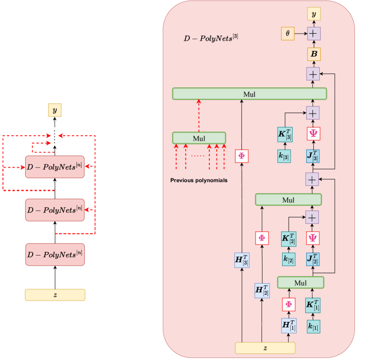
If we denote as $\bm{y}^{[i]}$ the output of the $i^{\text{th}}$ polynomial, then the recursive formulation of $\mathcal{D}$-PolyNets based on (1) is the following expressions:

$$\begin{split}\bm{y}_{n}^{[i]}=\bm{y}_{n-1}^{[i]}+\\ \left(\bm{\Phi}\bm{H}_{[n]}^{T}\bm{z}\right)*\left(\bm{\Psi}\bm{J}_{[n]}^{T}\bm{y}_{n-1}+\bm{K_{[n]}^{T}}\bm{k_{[n]}}\right)*_{\tau=1}^{i-1}\bm{y}^{[\tau]}.\end{split}$$ (3)

The total degree of expansion in Eq. (3) is higher than the corresponding one in $\mathcal{R}$-PolyNets or $\Pi$-Nets. This makes the requirement for strong regularization imperative to avoid exploding gradients.

Equation (1) enables us to build a regularized polynomial expansion of arbitrary degree, $\bm{y}_{n}$. Apart from the training techniques in sec 3.2, we propose below specific techniques to enforce a strong regularization of $\mathcal{D}$-PolyNets.

Training Configuration of $\mathcal{D}$-PolyNets: Our preliminary experiments indicate that iterative normalization [20] is beneficial in this case. Additionally, we include a learnable parameter $\rho_{\tau}$ which regularizes the contribution of each previous polynomial in the current Hadamard product.

5 Experiments

In this section, we evaluate the proposed models across a range of six in image recognition and one standard dataset in audio recognition. We describe below the datasets, and the setup, then we conduct an ablation study to evaluate the contribution of different techniques in sec. 5.1. Sequentially, we conduct the main body of the experiments in various widely-used datasets in sec. 5.2 and sec. 5.3. We extend beyond the standard image classification tasks, with audio classification and fine-grained classification in sec. 5.4 and sec. 5.5 respectively. Details on the datasets along with additional experiments (including an experiment with deeper networks and the runtime comparison in FLOPs) are developed in sec. D. The results in the supplementary verify the empirical findings below, while the the proposed $\mathcal{R}$-PolyNets has a similar number of FLOPs as the $\Pi$-Nets, e.g., in Table 21.

Figure 4: Accuracy on Cifar-100. The symbols ‘V0’, ‘V1’, ‘V2’ and ‘V3’ denote $\mathcal{R}$-PolyNets (IBN), $\mathcal{R}$-PolyNets (IBN + max pooling), $\mathcal{R}$-PolyNets (IBN + max pooling + Dropblock) and $\mathcal{R}$-PolyNets (IBN + max pooling + Dropblock + Label smoothing) respectively. Note that the normalization scheme adds a significant improvement, and similarly the regularized loss (i.e., Label smoothing) has also a considerable effect. Overall, training techniques such as Dropblock and Label smoothing improve the testing performance and obtain a result comparable to the baseline model (vanilla ResNet18).

Training details: Each model is trained for $120$ epochs with batch size $128$. The SGD optimizer is used with initial learning rate of $0.1$. The learning rate is multiplied with a factor of $0.1$ in epochs $40,60,80,100$. For Tiny ImageNet, the learning rates of $\mathcal{R}$-PolyNets and $\mathcal{D}$-PolyNets are multiplied by $0.92$ every epoch. For data augmentation we adopt random cropping with 4-pixel padding and horizontal flipping. Unless mentioned otherwise, each experiment is conducted 5 times and the average and the standard deviations are also reported.

Compared methods: The family of $\Pi$-Nets is the main baseline we use in our comparisons. Namely, the $\Pi$-Nets use the structure of ResNet18, where each block from the original ResNet is converted into a second-degree polynomial expansion. As a reminder, $\Pi$-Nets do not use element-wise activation functions, and result in a high-degree polynomial expansion. The recent PDC [4] is also added as a baseline with many of its properties shared with $\Pi$-Nets. We also report the accuracy of two further methods: (a) the popular ResNet18, which is the de facto baseline in image recognition, (b) hybrid $\Pi$-Nets, i.e., polynomial expansions with element-wise activation functions. The last two methods are added as a reference (thus added with grayscale color). Outperforming the vanilla ResNet18 or the hybrid $\Pi$-Nets is not our goal in this work. We aim at demonstrating for the first time that polynomial expansions can be on par with feed-forward neural networks.

5.1 Ablation study

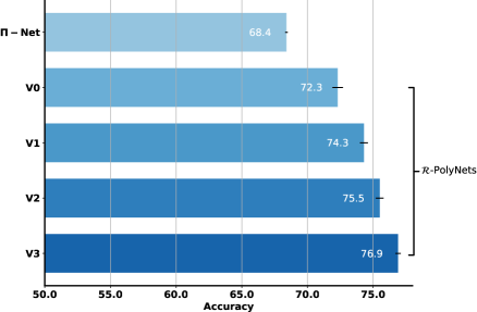
Below, we conduct three ablation experiments. In the first experiment, we showcase how the different components proposed in sec. 3 can decrease the error in image recognition. We choose Cifar-100 for this experiment. To facilitate the presentation, we gradually insert different regularization components on $\Pi$-Nets to advocate for stronger regularization techniques and highlight their benefit in the final accuracy.

Fig. 4 summarizes the results of the experiment. Notice that the initialization plus the normalization scheme already makes a significant impact on the accuracy. Then, max pooling, the feature augmentation and regularized loss contribute to reduce overfitting and to achieve the final performance. In the next experiments, we consider the last row of Fig. 4 as the model that is used for the main comparisons.

Table 2: Accuracy of $\mathcal{R}$-PolyNets (IBN + max pooling + Dropblock + Label smoothing) and $\mathcal{D}$-PolyNets (IBN + max pooling + Dropblock + Label smoothing) with different initialization schemes on Cifar-100. Note that $\mathcal{D}$-PolyNets contains $7$M parameters (down from the $11$M of $\mathcal{R}$-PolyNets) and one block less than $\mathcal{R}$-PolyNets.

Model	Initialization	Accuracy
$\mathcal{R}$-PolyNets	Xavier	$0.765\pm 0.002$
	Orthogonal	$0.765\pm 0.001$
	Kaiming normal	$0.767\pm 0.003$
	Kaiming uniform	$0.767\pm 0.004$
	zero-mean	$\bm{0.769\pm 0.002}$
$\mathcal{D}$-PolyNets	Xavier	$0.761\pm 0.004$
	Orthogonal	$0.764\pm 0.001$
	Kaiming normal	$0.764\pm 0.002$
	Kaiming uniform	$0.760\pm 0.004$
	zero-mean	$\bm{0.767\pm 0.003}$

In the second experiment, we utilize well-established initialization schemes, i.e., Xavier initialization [15], orthogonal matrix initialization [36], Kaiming initialization [16], and evaluate their performances on the proposed $\mathcal{R}$-PolyNets. The results in Table 2 indicate that previously proposed initializations cannot perform as well in the $\mathcal{R}$-PolyNets. This is not contradictory to the studies of those initialization schemes, since they were derived for the neural network structure, which differs substantially from the structure of PNs.

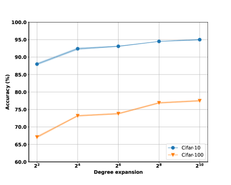
In the third experiment, we vary the degree of polynomials applied in $\mathcal{R}$-PolyNets. The results in Fig. 5 indicate that an increasing degree of polynomial expansion can increase the accuracy. Given the correspondence between the standard ResNet18 with $8$ residual blocks and the $2^{8}$ degree polynomial, we use this $2^{8}$ degree in the rest of the experiments unless explicitly stated otherwise.

Figure 5: Accuracy of $\mathcal{R}$-PolyNets with varying degree polynomials on Cifar-10 and Cifar-100.

5.2 Image classification on smaller datasets

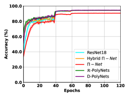
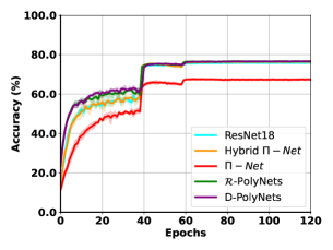
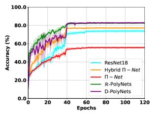
We conduct our main experimentation in the following four datasets: Cifar-10, Cifar-100, STL-10, Tiny ImageNet. Table 3 exhibits the accuracy of each compared method across all datasets. The results indicate that the $\mathcal{R}$-PolyNets consistently outperform the baseline $\Pi$-Nets by a large margin. In STL-10 the accuracy increases from $56.3\%$ to $82.8\%$, which is a $47.1\%$ relative increase in the performance. In Fig. 6 the test accuracy per epoch is depicted; notice that the proposed method has a consistently higher accuracy over the $\Pi$-Nets throughout the training. This consistent improvement demonstrates the efficacy of the proposed method. In Table 3, ResNet18 and hybrid $\Pi$-Nets are added. $\mathcal{R}$-PolyNets achieve a higher performance than ResNet18 and hybrid $\Pi$-Nets on the three benchmarks of Cifar-10, Cifar-100 and STL-10, while the three methods perform on par on Tiny ImageNet. These observations verify our proposal that regularized polynomials can achieve a similar performance with the standard baselines of neural networks or hybrid $\Pi$-Nets.

Table 3: Accuracy on Cifar-10, Cifar-100, STL-10 and Tiny ImageNet. The symbol ‘# par’ abbreviates the number of parameters. $\mathcal{D}$-PolyNets containing 7M parameters. Note that $\mathcal{R}$-PolyNets and $\mathcal{D}$-PolyNets without activation functions can outperform $\Pi$-Nets without activation functions significantly on Cifar-10, Cifar-100, STL-10 and Tiny ImageNet. Moreover, $\mathcal{R}$-PolyNets and $\mathcal{D}$-PolyNets can match the performances of baseline models (e.g. $\Pi$-Nets with activation functions and ResNet18) on Cifar-10, Cifar-100 and STL-10.

Dataset	Model	# par	Accuracy
Cifar-10	ResNet18	$11.2$M	$0.944\pm 0.001$
	Hybrid $\Pi$-Nets	$6.0$M	$0.944\pm 0.002$
	PDC	$5.4$M	$0.909\pm 0.002$
	$\Pi$-Nets	$11.9$M	$0.907\pm 0.003$
	$\mathcal{R}$-PolyNets	$11.9$M	$0.945\pm 0.000$
	$\mathcal{D}$-PolyNets	$7.1$M	$\bm{0.947\pm 0.002}$
Cifar-100	ResNet18	$11.2$M	$0.760\pm 0.003$
	Hybrid $\Pi$-Nets	$6.1$M	$0.765\pm 0.004$
	PDC	$5.5$M	$0.689\pm 0.002$
	$\Pi$-Nets	$11.9$M	$0.677\pm 0.006$
	$\mathcal{R}$-PolyNets	$11.9$M	$\bm{0.769\pm 0.002}$
	$\mathcal{D}$-PolyNets	$7.2$M	$0.767\pm 0.003$
STL-10	ResNet18	$11.2$M	$0.741\pm 0.016$
	Hybrid $\Pi$-Nets	$6.0$M	$0.775\pm 0.006$
	PDC	$5.4$M	${0.681\pm 0.006}$
	$\Pi$-Nets	$11.9$M	${0.563\pm 0.008}$
	$\mathcal{R}$-PolyNets	$11.9$M	$0.828\pm 0.003$
	$\mathcal{D}$-PolyNets	$7.1$M	$\bm{0.834\pm 0.006}$
Tiny ImageNet	ResNet18	$11.3$M	$0.615\pm 0.002$
	Hybrid $\Pi$-Nets	$6.1$M	$0.611\pm 0.004$
	PDC	$5.5$M	$0.452\pm 0.002$
	$\Pi$-Nets	$12.0$M	$0.502\pm 0.007$
	$\mathcal{R}$-PolyNets	$12.0$M	$0.615\pm 0.004$
	$\mathcal{D}$-PolyNets	$7.2$M	$\bm{0.618\pm 0.001}$

(a)

(b)

(c)

Figure 6: Test error on (a) Cifar-10, (b) Cifar-100 and (c) STL-10. The highlighted region depicts the variance in the accuracy. Interestingly, the proposed $\mathcal{R}$-PolyNets and $\mathcal{D}$-PolyNets outperform the $\Pi$-Nets from the first few epochs, while the absolute difference in the error is not decreasing as the training progresses. Notice that the proposed training techniques enable $\mathcal{R}$-PolyNets and $\mathcal{D}$-PolyNets to be on par with the ResNet18 baseline in STL-10 and even outperform the baselines in Cifar-100.

Table 4: ImageNet classification results. We compare our models with state-of-the-art deep convolutional neural networks, $\Pi$-Nets and hybrid $\Pi$-Nets. We report the top-1 and top-5 accuracy on the validation set of ImageNet as well as the number of parameters. Our models are highlighted in gray. The symbol ‘# par’ abbreviates the number of parameters.

Model	Image Size	# par $(\mathrm{M})$	Top-1 Acc. $(\%)$	Top-5 Acc. $(\%)$
ImageNet-1K trained models
ResNet18	$224^{2}$	$11.69$	$69.758$	$89.078$
ResNet18 without activations	$224^{2}$	$11.69$	$20.536$	$39.986$
Hybrid $\Pi$-Nets	$224^{2}$	$11.96$	$\bm{70.740}$	$\bm{89.548}$
$\Pi$-Nets	$224^{2}$	$12.38$	$65.280$	$85.958$
$\mathcal{R}$-PolyNets	$224^{2}$	$12.38$	$70.228$	$89.390$
$\mathcal{D}$-PolyNets	$224^{2}$	$11.36$	$70.090$	$89.424$

Discussion on $\mathcal{R}$-PolyNets: A reasonable question would be whether the studied training techniques are unique in enabling the training of $\mathcal{R}$-PolyNets. Our preliminary experiments with alternative methods indicate that different combinations of training techniques can indeed perform well. However, the proposed techniques are the only ones we found that perform well in a range of datasets. To verify this, we conducted two experiments to assess alternative training techniques of $\mathcal{R}$-PolyNets.

In the first experiment, we increase the weight decay to train $\mathcal{R}$-PolyNets on Cifar-100. We notice that max pooling and Label smoothing can prevent $\mathcal{R}$-PolyNets from overfitting the train samples. However, the alternative regularization schemes may also help $\mathcal{R}$-PolyNets achieve the similar final performance. To verify this, we conduct another experiment of training $\mathcal{R}$-PolyNets with different regularization techniques. The result is presented in Table 6.

As the results in Table 5 and Table 6 illustrate, different combinations of regularization techniques can indeed improve the test performance of $\mathcal{R}$-PolyNets. Notice that the CutMix and Stochastic depth can also help PN without element-wise activation functions perform on par with established DNNs. However, we find their behavior is dataset-dependent, so we do not include them in our final scheme.

Discussion on $\mathcal{D}$-PolyNets: The results in Table 3 demonstrate that $\mathcal{D}$-PolyNets can match the test performance of $\mathcal{R}$-PolyNets, which both outperform the baseline $\Pi$-Nets. However, $\mathcal{D}$-PolyNets have $41.7\%$ fewer parameters. The representation power of $\mathcal{D}$-PolyNets is improved, because the total degree of polynomial expansion output by $\mathcal{D}$-PolyNets can reach $\bm{z}^{588}$ higher than that of $\Pi$-Nets ($\bm{z}^{256}$) when they use at most $8$ blocks each. The results validate our assumption that $\mathcal{D}$-PolyNets are more expressive.

Table 5: The impact of weight decay changes on $\mathcal{R}$-PolyNets (IBN + max pooling + Dropblock + Label smoothing) trained on Cifar-100.

Weight decay	Accuracy
$5e^{-4}$	$0.766\pm 0.002$
$6e^{-4}$	$0.768\pm 0.004$
$7e^{-4}$	$\bm{0.768\pm 0.002}$

Table 6: Accuracy on Cifar-100. Note that Data aumentation (i.e. Cutmix) can achieve the best test performance. Overall, these alternative training techniques obtain a state-of-the-art result with respect to the baseline model (ResNet18).

Models	Accuracy
$\mathcal{R}$-PolyNets (IBN + maxpooling + Dropblock + Label smoothing)	$0.766\pm 0.002$
$\mathcal{R}$-PolyNets (IBN + maxpooling + Dropblock + CutMix)	$\bm{0.771\pm 0.002}$
$\mathcal{R}$-PolyNets (IBN + maxpooling + Stochastic depth + Label smoothing)	$0.769\pm 0.002$

5.3 ImageNet Classification

We conduct a large-scale classification experiment on ImageNet [10]. We employ the mmclassification toolkit [9] to train networks on the training set and report the $224\times 224$ single-crop top-1 and the top-5 errors on the validation set. Our pre-processing and augmentation strategy follows the settings of the baseline (i.e., ResNet18). All models are trained for 100 epochs on 8 GPUs with 32 images per GPU (effective batch size of 256) with synchronous SGD of momentum 0.9. The learning rate is initialized to 0.1, and decays by a factor of 10 at the $30^{\text{th}}$, $60^{\text{th}}$, and $90^{\text{th}}$ epochs. The results in Table 4 validate our findings on the rest of the datasets and confirm that $\mathcal{R}$-PolyNets are able to reach the performance of standard neural network baselines. $\mathcal{D}$-PolyNets perform on par with $\mathcal{R}$-PolyNets, while having a slightly reduced number of parameters. The reduction in parameters is smaller than the respective numbers with smaller scale datasets (e.g., Table 3) , which might indicate that further regularization is required for $\mathcal{D}$-PolyNets when scaled to more complex datasets.

5.4 Audio classification

We perform an experiment on the Speech Commands dataset to evaluate $\mathcal{R}$-PolyNets and $\mathcal{D}$-PolyNets on a distribution that differs from that of natural images. The accuracy for each model is reported in Table 7. Noticeably, hybrid $\Pi$-Nets, $\mathcal{R}$-PolyNets, $\mathcal{D}$-PolyNets and ResNet18 can achieve the accuracy over $0.975$, which showcases the representative power of $\mathcal{R}$-PolyNets and $\mathcal{D}$-PolyNets on audio classification. By comparison, $\Pi$-Nets and PDC has accuracy below $0.975$.

Table 7: Accuracy on Speech Command. Note the Hybrid $\Pi$-Nets, $\mathcal{R}$-PolyNets, $\mathcal{D}$-PolyNets and ResNet18 can achieve the same test performance.

Dataset	Model	# par	Accuracy
Speech command	ResNet18	$11.2$M	$0.977$
	Hybrid $\Pi$-Nets	$6.0$M	$0.977$
	PDC	$5.4$M	$0.972$
	$\Pi$-Nets	$11.9$M	$0.972$
	$\mathcal{R}$-PolyNets	$11.9$M	$0.977$
	$\mathcal{D}$-PolyNets	$7.2$M	$0.977$

5.5 Fine-grained classification

We conduct one last experiment on fine-grained classification to validate further the regularization scheme of $\mathcal{R}$-PolyNets. We select the Oxford $102$ Flowers dataset [32], which contains $102$ flower categories with $10$ training images and $10$ validation images annotated per class. The accuracy for each model is exhibited in Table 8, where $\mathcal{R}$-PolyNets performs favorably to the vanilla ResNet18. As a reminder, the goal of our experiments is not to demonstrate state-of-the-art behavior, but rather to focus on achieving performance at least comparable to the existing DNNs.

Table 8: Accuracy on Oxford 102 Flowers. Note $\mathcal{R}$-PolyNets and $\mathcal{D}$-PolyNets perform favorably to the vanilla ResNet18.

Dataset	Model	# par	Accuracy
Oxford Flower	ResNet18	$11.2$M	$0.877$
	Hybrid $\Pi$-Nets	$6.1$M	$0.889$
	PDC	$5.5$M	$0.885$
	$\Pi$-Nets	$11.9$M	$0.826$
	$\mathcal{R}$-PolyNets	$11.9$M	$\bm{0.949}$
	$\mathcal{D}$-PolyNets	$7.2$M	$0.941$

6 Conclusion

In this work, we focus on Polynomial Nets (PNs) for image recognition. We propose a new parametrization of PNs that enables them to avoid reported overfitting issues using custom initialization and normalization schemes. We showcase how the proposed model, called $\mathcal{R}$-PolyNets, extends previously proposed PN models. Our thorough evaluation with six datasets exhibits a significant improvement over previously proposed PN models and establish $\mathcal{R}$-PolyNets as an alternative to existing DNNs. Furthermore, we introduce $\mathcal{D}$-PolyNets that leverage dense connections across sequential polynomials to capture higher-order correlations. Experimentally, $\mathcal{D}$-PolyNets verify their expressivity over alternative PNs. We believe that our work can encourage further research in alternative models for image recognition.

Limitations: A deeper theoretical understanding of PNs is needed, particularly regarding the link between the degree, the regularization requirements and the generalization error. Concretely, each block of polynomials we are using is composed of lower-degree polynomial expansions. We hypothesize that the high-degree obtained from the sequential polynomial blocks might be sufficient for image recognition tasks, but might not suffice for harder tasks. In addition, the theoretical study of the initialization or the regularization requirements on PNs remains elusive.

Contents of the Appendix

The following sections are included in the appendix:

• A review of the $\Pi$-Nets is in sec. A.

• An alternative parameterization to $\mathcal{R}$-PolyNets is introduced in sec. B.

• A number of auxiliary tables and visualizations that could not fit in the main paper are in sec. C.

• Lastly, a number of additional experiments are conducted in sec. D.

Appendix A Background: $\Pi$-Nets

$\Pi$-Nets is a family of architectures that are high-degree polynomial expansions [5]. To reduce the parameters and enable the implementation of the polynomial expansion, coupled tensor decompositions are utilized. This results in a simple recursive formulation that enables an arbitrary degree of expansion. For instance, the $N^{\text{th}}$ degree polynomial used for image recognition is expressed as:

$$\bm{y}_{1}=\left(\bm{H}_{[1]}^{T}\bm{z}\right)*\left(\bm{K}_{[1]}^{T}\bm{k}_{[1]}\right),$$ (4)

$$\bm{y}_{n}=\left(\bm{H}_{[n]}^{T}\bm{z}\right)*\left(\bm{J}_{[n]}^{T}\bm{y}_{n-1}+\bm{K}_{[n]}^{T}\bm{k}_{[n]}\right)+\bm{y}_{n-1},$$ (5)

$$\bm{y}=\bm{B}\bm{y}_{N}+\bm{\theta},$$ (6)

for $n=2,\ldots,N$. The symbol $\bm{z}$ is the input vector of the polynomial, $\bm{y}$ is the output. The parameters $\bm{B},\bm{\theta},\{\bm{H}_{[n]},\bm{J}_{[n]},\bm{K}_{[n]},\bm{k}_{[n]}\}_{n=1}^{N}$ are trainable. The aforementioned models can be used both in a hybrid setting (i.e., using polynomial expansion with element-wise activation) functions or as polynomial expansions. In the latter case, it was reported that despite the training accuracy reaching $100\%$, the testing accuracy was reduced when compared to DNNs.

Appendix B CCP-equivalent for the regularized model

Beyond the aforementioned model of sec. 3.1, by changing the assumptions behind the tensor decomposition, one could retrieve another architecture. In this section, we demonstrate how an alternative parametrization, called CCP in [5] can be reformulated in our context. A coupled CP decomposition (CCP) can be used for tensor parameters of PNs. The recursive equation of CCP can be expressed as:

$$\bm{y}_{1}=\bm{H}_{[1]}^{T}\bm{z},$$

$$\bm{y}_{n}=\left(\bm{H}_{[n]}^{T}\bm{z}\right)*\bm{y}_{n-1}+\bm{y}_{n-1},$$

$$\bm{y}=\bm{B}\bm{y}_{N}+\theta,$$

for $n=1,\ldots,N$, the parameters $\bm{B}\in\mathbb{R}^{o\times r},\bm{H}_{[n]}\in\mathbb{R}^{d\times r}$ for $n=1,\ldots,N$ are trainable.

After introducing regularization matrix, $\bm{\Phi}\in\mathbb{R}^{r\times r}$, the modified recursive relationships for $n=2,\ldots,N$ can be expressed as follows:

$$x_{n}=\left(\bm{\bm{\Phi}}\bm{H}_{[n]}^{T}\bm{z}\right)*\bm{y}_{n-1}+\bm{y}_{n-1}.$$

A schematic assuming a third order expansion ($N=3$) is illustrated in Fig. 7.

Figure 7: Schematic illustration of the regularized CCP (for third degree approximation). Symbol $*$ refers to the Hadamard product.

Table 9: Experimental settings in sec 5.2 and sec 5.3. Note the hyper-parameters of label smoothing are selected on the validation sets of Cifar-10 and Cifar-100.

	Cifar-10/Cifar-100/STL-10/Tiny ImageNet	ImageNet
optimizer	SGD	SGD
base learning rate	$1\mathrm{e}-1$	$1\mathrm{e}-1$
weight decay	$5\mathrm{e}-4$	$1\mathrm{e}-4$
optimizer momentum	$0.9$	$0.9$
batch size	$128$ ($64$: Tiny ImageNet)	$256$
training epochs	$120$	$100$
learning rate schedule	multi-step decay	multi-step decay
	exponential decay: $\mathcal{R}$-PolyNets/ $\mathcal{D}$-PolyNets (Tiny ImageNet)
label smoothing: $\mathcal{R}$-PolyNets/$\mathcal{D}$-PolyNets	$0.1$: (Cifar-10 and STL-10)	$0.1$
	$0.4$: (Cifar-100)
	$0.6$: (Tiny ImageNet)

Table 10: Experimental setting in sec 5.4.

	Speech Command
optimizer	SGD
base learning rate	$1\mathrm{e}-1$
weight decay	$5\mathrm{e}-4$
optimizer momentum	$0.9$
batch size	$128$
training epochs	$120$
learning rate schedule	multi-step decay
label smoothing: $\mathcal{R}$-PolyNets/$\mathcal{D}$-PolyNets	$0.1$

Table 11: Experimental setting in sec 5.5.

	Oxford $102$ Flowers
optimizer	SGD
base learning rate	$1\mathrm{e}-1$
weight decay	$5\mathrm{e}-4$
optimizer momentum	$0.9$
batch size	$64$
training epochs	$120$
learning rate schedule	multi-step decay
label smoothing: $\mathcal{R}$-PolyNets/$\mathcal{D}$-PolyNets	$0.4$

Appendix C Auxiliary tables and visualizations for experiments on the main paper

Below we list the settings for experiments on the main paper in the Table 9, Table 10 and Table 11. The Table 12 ablates the accuracy for different degree polynomials on Cifar-10 and Cifar-100.

Table 12: Accuracy of $\mathcal{R}$-PolyNets with varying degree polynomials on Cifar-10 and Cifar-100. Each block is a degree $2$ polynomial expansion, which results in the $2^{6}$ expansion if we add $6$ such blocks. Blocks with higher-degree can also be used, however we note that training those has not been as stable in our experience.

Dataset	Degree polynomials	Accuracy
Cifar-10	$2^{2}$ degree expansion	$0.880\pm 0.003$
	$2^{4}$ degree expansion	$0.924\pm 0.003$
	$2^{6}$ degree expansion	$0.931\pm 0.001$
	$2^{8}$ degree expansion	$0.945\pm 0.000$
	$2^{10}$ degree expansion	$\bm{0.950\pm 0.002}$
Cifar-100	$2^{2}$ degree expansion	$0.671\pm 0.003$
	$2^{4}$ degree expansion	$0.732\pm 0.002$
	$2^{6}$ degree expansion	$0.738\pm 0.002$
	$2^{8}$ degree expansion	$0.769\pm 0.002$
	$2^{10}$ degree expansion	$\bm{0.775\pm 0.002}$

Appendix D Additional experimental results

The following additional experimental results are added below:

1. We evaluate the classification under limited training data in sec. D.1.

2. We conduct an error analysis for best and worst performing classes in sec. D.2.

3. In sec. D.3, an comparison with convolutional kernel networks is conducted.

Below, we also add details on the datasets used in this paper:

Datasets: The following datasets are used in our evaluation:

1. Cifar-10 [22] is a popular image recognition dataset consisting of $50,000$ training and $10,000$ testing images evenly distributed across $10$ classes. Each image is of resolution $32\times 32$.

2. Cifar-100 [23] includes images similar to Cifar-10. Cifar-100 contains $100$ object classes with $600$ ($500$ for training, $100$ for testing) images annotated per class.

3. STL-10 [7] contains $10$ object classes that are similar to Cifar-10. Each image is of resolution $96\times 96$, while the dataset contains $5,000$ images. This dataset is used to evaluate the performance on images of higher resolution, while using limited data.

4. Tiny ImageNet [25] contains $200$ object classes, where each image is of resolution $64\times 64$. There are $500$ images annotated per class, while the object classes demonstrate a larger variance than the aforementioned datasets.

5. Speech Commands dataset [46] includes $60,000$ audio files; each audio contains a single word of a duration of one second. There are $35$ different words (classes) with each word having $1,500-4,100$ recordings. Every audio file is converted into a mel-spectrogram of resolution $32\times 32$.

6. ImageNet Large Scale Visual Recognition Challenge 2012 (ILSVRC2012) [10] contains over one million training images and $50,000$ validation images from $1,000$ object classes. Each image depicts natural scenes and is annotated with a single object per image.

D.1 Image classification with limited data

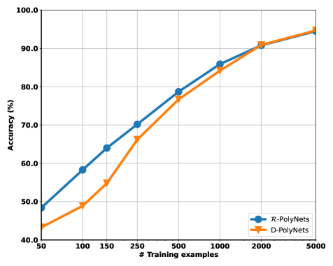
We conduct an experiment on Cifar-10 in the presence of limited data. The hyper-parameters in sec. 5.2 are used unchanged, while only the number of training samples of each class is reduced. The results in Table 13 exhibit that $\mathcal{R}$-PolyNets outperform $\Pi$-Nets in the presence of limited training data. Notice that in the extreme case of only $50$ samples per class, there is a relative increase of $50\%$ from the accuracy of $\Pi$-Nets. The goal of this experiment is to explore how $\Pi$-Nets and $\mathcal{D}$-PolyNets perform in the presence of limited data. Indeed, Fig. 8 confirms that both networks perform reasonably in the case of limited data.

Table 13: Accuracy of image classification with limited data on Cifar-10. Note that $\mathcal{R}$-PolyNets without activation functions can outperform $\Pi$-Nets without activation functions significantly on limited data of Cifar-10.

Training samples per class	$\Pi$-Nets	$\mathcal{R}$-PolyNets
$50$	$0.314\pm 0.005$	$\bm{0.484\pm 0.004}$
$100$	$0.355\pm 0.010$	$\bm{0.583\pm 0.003}$
$150$	$0.396\pm 0.010$	$\bm{0.640\pm 0.006}$

Figure 8: Image classification with limited data on Cifar-10. The x-axis declares the number of training samples per class (log-axis).

D.2 Error Analysis

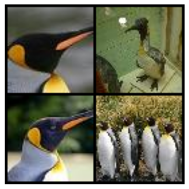
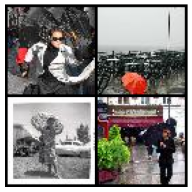
We use our best-performing $\mathcal{R}$-PolyNets to calculate per-class error rates for all 200 classes on the validation dataset of a large-scale classification dataset, Tiny ImageNet [25]. We report the top-5 accurate and misclassified classes in Table 14. Also, we present the images of the most accurate class (king penguin) and the most misclassified class (umbrella) in Fig. 9.

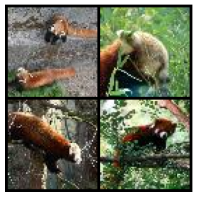
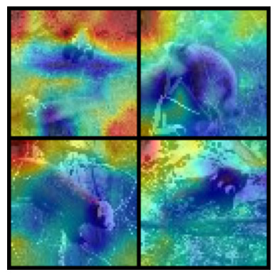
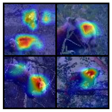
Remarkably, $\mathcal{R}$-PolyNets achieve above $85\%$ validation accuracy for the top-5 accurate classes. We analyse the images of the most accurate class and misclassified class. As shown in Fig. 9, the king penguins occupy most regions in the images. Also, they have similar shape, color and texture. On the other side, the umbrellas in Fig. 9 have different colors and shapes. Furthermore, the images are dominated by the other objects such as human beings and landscape. The saliency maps in Fig. 10 computed by GradCAM [38] indicate $\mathcal{R}$-PolyNets can concentrate on the main object in an image. By comparison, $\Pi$-Nets recognize the lesser panda at $92.7\%$ accuracy, but the saliency maps in Fig. 10 show $\Pi$-Nets do not concentrate on the main object in an image.

Table 14: Top-5 Accurate/Misclassified Classes on Tiny ImageNet. Note that $\mathcal{R}$-PolyNets can achieve above $85\%$ validation accuracy for the top-5 accurate classes.

Class Name	Accuracy	Class Name	Accuracy
king penguin	$0.902$	backpack	$0.358$
lesser panda	$0.900$	bucket	$0.327$
sea slug	$0.895$	plunger	$0.296$
bullet train	$0.882$	wooden spoon	$0.278$
Persian cat	$0.879$	umbrella	$0.243$

(a)

(b)

Figure 9: Images of the Most Accurate/Misclassified Class recognized by $\mathcal{R}$-PolyNets. As in Fig 9, the king penguins in (a) have similar characteristics, and occupy most regions in the images. On the other side, the images in (b) are dominated by other objects such as persons and landscape.

(a)

(b)

(c)

(d)

Figure 10: Saliency maps of $\Pi$-Nets and $\mathcal{R}$-PolyNets. As in Fig 10, $\Pi$-Nets can recognize the lesser panda in (a) at $93\%$ accuracy, but the saliency maps in (b) indicate $\Pi$-Nets can not concentrate on the main object in an image. The saliency maps in (d) indicate $\mathcal{R}$-PolyNets can concentrate on the main object in an image.

D.3 Comparison with convolutional kernel networks

We conduct experiments to compare $\mathcal{R}$-PolyNets and $\mathcal{D}$-PolyNets with supervised convolutional kernel networks (SCKNs) [29], which is among the principled design choices. The results of $\mathcal{R}$-PolyNets and $\mathcal{D}$-PolyNets are the same as those in the main paper, i.e., in Table 3. The accuracy for each model is reported in Table 15. Notice that the proposed $\mathcal{R}$-PolyNets and $\mathcal{D}$-PolyNets outpuperform the newly added baseline.

Table 15: Accuracy on Cifar-10, Cifar-100, STL-10 and Tiny ImageNet. The symbol ‘# par’ abbreviates the number of parameters. $\mathcal{D}$-PolyNets containing 7M parameters. Note that $\mathcal{R}$-PolyNets and $\mathcal{D}$-PolyNets without activation functions can outperform SCKNs on Cifar-10, Cifar-100, STL-10 and Tiny ImageNet by a large margin.

Dataset	Model	# par	Accuracy
Cifar-10	SCKNs	$3.4$M	$0.895\pm 0.002$
	$\mathcal{R}$-PolyNets	$11.9$M	$0.945\pm 0.000$
	$\mathcal{D}$-PolyNets	$7.1$M	$\bm{0.947\pm 0.002}$
Cifar-100	SCKNs	$3.5$M	$0.610\pm 0.003$
	$\mathcal{R}$-PolyNets	$11.9$M	$\bm{0.769\pm 0.002}$
	$\mathcal{D}$-PolyNets	$7.2$M	$0.767\pm 0.003$
STL-10	SCKNs	$3.4$M	${0.527\pm 0.012}$
	$\mathcal{R}$-PolyNets	$11.9$M	$0.828\pm 0.003$
	$\mathcal{D}$-PolyNets	$7.1$M	$\bm{0.834\pm 0.006}$
Tiny ImageNet	SCKNs	$4.2$M	$0.409\pm 0.001$
	$\mathcal{R}$-PolyNets	$12.0$M	$0.615\pm 0.004$
	$\mathcal{D}$-PolyNets	$7.2$M	$\bm{0.618\pm 0.001}$

D.4 Regularized PDC, ResNext and dense connections for PDC

To showcase the representative power of the regularized polynomial expansion and dense connections across different polynomial nets, we firstly apply the proposed regularization schemes (IBN + max pooling + Dropblock + Label smoothing) in the influential ResNext [48] and the recent PDC [4]. The regularized ResNext is called $\mathcal{R}$-PolyNeXt, while the regularized PDC is called $\mathcal{R}$-PDC. The results for ResNext are reported in Table 18. Even though $\mathcal{R}$-PolyNeXt performs on par with ResNext, we notice that there is some training instability that did not emerge in regularizing PDC or $\Pi$-Nets. It is possible that further tuning is required for converting more complex models, such as ResNext, into polynomial expansions.

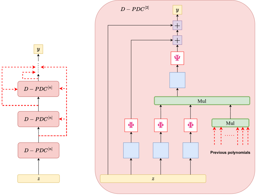
Furthermore, we also enable additional skip connections across polynomials for PDC. The new type of PDC is called $\mathcal{D}$-PDC. The schematic in Fig. 11 depicts $\mathcal{D}$-PDC assuming each polynomial includes a single recursive step. This can be trivially extended to any number of recursive steps, while each polynomial can also rely on a different tensor decomposition. The same regularization scheme (IBN + max pooling + Dropblock + Label smoothing) in $\mathcal{D}$-PolyNets is used in $\mathcal{D}$-PDC. The accuracy for each model is reported in Table 16. Notice that the $\mathcal{R}$-PDC and $\mathcal{D}$-PDC both outperform the PDC. The rest of the patterns, e.g., $\mathcal{D}$-PDC versus $\mathcal{R}$-PDC, are similar to the experiments in the main paper.

Figure 11: Schematic illustration of $\mathcal{D}$-PDC. On the left the overall structure is presented, while on the right a single second-degree polynomial using the structure of $\mathcal{D}$-PDC is visualized. The red arrows depict the newly added connections with respect to previous polynomial expansions.

Table 16: Accuracy on Cifar-10, Cifar-100, STL-10 and Tiny ImageNet. The symbol ‘# par’ abbreviates the number of parameters. Note that $\mathcal{R}$-PDC and $\mathcal{D}$-PDC without activation functions can outperform PDC without activation functions significantly on Cifar-10, Cifar-100, STL-10 and Tiny ImageNet.

Dataset	Model	# par	Accuracy
Cifar-10	PDC	$5.4$M	$0.909\pm 0.002$
	$\mathcal{R}$-PDC	$7.3$M	$0.947\pm 0.001$
	$\mathcal{D}$-PDC	$6.0$M	$\bm{0.949\pm 0.002}$
Cifar-100	PDC	$5.5$M	$0.689\pm 0.002$
	$\mathcal{R}$-PDC	$7.4$M	$0.757\pm 0.003$
	$\mathcal{D}$-PDC	$6.0$M	$\bm{0.762\pm 0.001}$
STL-10	PDC	$5.4$M	${0.681\pm 0.006}$
	$\mathcal{R}$-PDC	$7.3$M	${0.833\pm 0.007}$
	$\mathcal{D}$-PDC	$6.0$M	$\bm{0.855\pm 0.003}$
Tiny ImageNet	PDC	$5.5$M	$0.452\pm 0.002$
	$\mathcal{R}$-PDC	$7.4$M	$0.560\pm 0.005$
	$\mathcal{D}$-PDC	$6.0$M	$\bm{0.569\pm 0.002}$

Table 17: Accuracy of $\mathcal{D}$-PolyNets without IBN and without label smoothing (mentioned as ‘$\mathcal{D}$-PolyNets without reg’ below) on Cifar-10 and Cifar-100. The symbol ‘# par’ abbreviates the number of parameters.

Dataset	Model	# par	Accuracy
Cifar-10	$\Pi$-Nets	$11.9$M	$0.907\pm 0.003$
	$\mathcal{D}$-PolyNets without reg	$7.1$M	$\bm{0.934\pm 0.002}$
Cifar-100	$\Pi$-Nets	$11.9$M	$0.677\pm 0.006$
	$\mathcal{D}$-PolyNets without reg	$7.2$M	$\bm{0.726\pm 0.006}$

Table 18: Accuracy of ResNext [48] and the corresponding $\mathcal{R}$-PolyNeXt on Cifar-10 and Cifar-100.

Dataset	Model	# par	Accuracy
Cifar-10	ResNeXt-$29$, $8\times 64$d	$34.4$M	$0.964$
	$\mathcal{R}$-PolyNeXt-$29$, $8\times 64$d	$38.6$M	$\bm{0.965}$
Cifar-100	ResNeXt-$29$, $8\times 64$d	$34.4$M	$0.822$
	$\mathcal{R}$-PolyNeXt-$29$, $8\times 64$d	$38.7$M	$\bm{0.824}$

D.5 Comparison with deeper ResNets

We conduct experiments to compare deeper $\mathcal{R}$-PolyNets and $\mathcal{D}$-PolyNets with deeper ResNets. The experimental settings described in sec. 5.2 remain unchanged for these comparisons. The accuracy for each model is reported in Table 19. It is noteworthy that the proposed $\mathcal{R}$-PolyNets and $\mathcal{D}$-PolyNets outperform ResNets when their architectures are deeper.

Table 19: Accuracy on Cifar-10 and Cifar-100. The symbol ‘# par’ abbreviates the number of parameters. Note that deeper $\mathcal{R}$-PolyNets and $\mathcal{D}$-PolyNets without activation functions can outperform deeper ResNets on Cifar-10, and Cifar-100.

Dataset	Model	# par	Accuracy
Cifar-10	ResNet34	$21.3$M	$0.947\pm 0.002$
	$\mathcal{R}$-PolyNets34	$22.5$M	$0.950\pm 0.001$
	$\mathcal{D}$-PolyNets34	$13.5$M	$\bm{0.951\pm 0.002}$
	ResNet152	$58.2$M	$0.943\pm 0.003$
	$\mathcal{R}$-PolyNets152	$58.5$M	$0.952\pm 0.001$
	$\mathcal{D}$-PolyNets152	$54.2$M	$\bm{0.953\pm 0.002}$
Cifar-100	ResNet34	$21.3$M	$0.762\pm 0.004$
	$\mathcal{R}$-PolyNets34	$22.6$M	$\bm{0.788\pm 0.002}$
	$\mathcal{D}$-PolyNets34	$13.5$M	$0.787\pm 0.001$
	ResNet152	$58.3$M	$0.768\pm 0.005$
	$\mathcal{R}$-PolyNets152	$58.5$M	$\bm{0.793\pm 0.004}$
	$\mathcal{D}$-PolyNets152	$54.2$M	$0.791\pm 0.001$

D.6 FLOPs

We compute the floating-point operations per second (FLOPs) for $\mathcal{R}$-PolyNets, $\mathcal{D}$-PolyNets, $\Pi$-Nets, and ResNet18 on both small datasets and ImageNet. The results of these computations are presented in Table 20 and Table 21. Notice that the proposed $\mathcal{R}$-PolyNets has a similar FLOP as the previously proposed $\Pi$-Nets, while $\mathcal{D}$-PolyNets has only a marginal increase in the FLOPs.

Table 20: FLOPs on Cifar-10, Cifar-100, STL-10 and Tiny ImageNet.

Dataset	Model	GFLOPs
Cifar-10	ResNet18	$0.56$
	Hybrid $\Pi$-Nets	$0.46$
	$\Pi$-Nets	$0.59$
	$\mathcal{R}$-PolyNets	$0.59$
	$\mathcal{D}$-PolyNets	$0.55$
Cifar-100	ResNet18	$0.56$
	Hybrid $\Pi$-Nets	$0.46$
	$\Pi$-Nets	$0.59$
	$\mathcal{R}$-PolyNets	$0.59$
	$\mathcal{D}$-PolyNets	$0.55$
STL-10	ResNet18	$5.01$
	Hybrid $\Pi$-Nets	$4.11$
	$\Pi$-Nets	$5.31$
	$\mathcal{R}$-PolyNets	$5.31$
	$\mathcal{D}$-PolyNets	$4.94$
Tiny ImageNet	ResNet18	$2.23$
	Hybrid $\Pi$-Nets	$1.83$
	$\Pi$-Nets	$2.36$
	$\mathcal{R}$-PolyNets	$2.36$
	$\mathcal{D}$-PolyNets	$2.19$

Table 21: FLOPs on ImageNet. Notice that the proposed $\mathcal{R}$-PolyNets has a similar FLOP as the previously proposed $\Pi$-Nets.

Model	GFLOPs
ImageNet-1K trained models
ResNet18	$1.82$
ResNet18 without activations	$1.82$
Hybrid $\Pi$-Nets	$1.92$
$\Pi$-Nets	$1.92$
$\mathcal{R}$-PolyNets	$1.92$
$\mathcal{D}$-PolyNets	$1.98$

References

- [1] Francesca Babiloni, Ioannis Marras, Filippos Kokkinos, Jiankang Deng, Grigorios G Chrysos, and Stefanos Zafeiriou. Poly-nl: Linear complexity non-local layers with polynomials. In International Conference on Computer Vision (ICCV), 2021.
- [2] Olivier Chapelle, Jason Weston, Léon Bottou, and Vladimir Vapnik. Vicinal risk minimization. In Advances in neural information processing systems (NeurIPS), pages 416–422, 2001.
- [3] Moulik Choraria, Leello Tadesse Dadi, Grigorios G Chrysos, Julien Mairal, and Volkan Cevher. The spectral bias of polynomial neural networks. In International Conference on Learning Representations (ICLR), 2022.
- [4] Grigorios G Chrysos, Markos Georgopoulos, Jiankang Deng, Jean Kossaifi, Yannis Panagakis, and Anima Anandkumar. Augmenting deep classifiers with polynomial neural networks. In European Conference on Computer Vision (ECCV), 2022.
- [5] Grigorios G Chrysos, Stylianos Moschoglou, Giorgos Bouritsas, Yannis Panagakis, Jiankang Deng, and Stefanos Zafeiriou. nets: Deep polynomial neural networks. In Conference on Computer Vision and Pattern Recognition (CVPR), 2020.
- [6] Dan Ciregan, Ueli Meier, and Jürgen Schmidhuber. Multi-column deep neural networks for image classification. In Conference on Computer Vision and Pattern Recognition (CVPR), pages 3642–3649. IEEE, 2012.
- [7] Adam Coates, Andrew Ng, and Honglak Lee. An analysis of single-layer networks in unsupervised feature learning. In Proceedings of the fourteenth international conference on artificial intelligence and statistics, pages 215–223. JMLR Workshop and Conference Proceedings, 2011.
- [8] Michael Cogswell, Faruk Ahmed, Ross Girshick, Larry Zitnick, and Dhruv Batra. Reducing overfitting in deep networks by decorrelating representations. In International Conference on Learning Representations (ICLR), 2016.
- [9] MMClassification Contributors. Openmmlab’s image classification toolbox and benchmark. https://github.com/open-mmlab/mmclassification, 2020.
- [10] Jia Deng, Wei Dong, Richard Socher, Li-Jia Li, Kai Li, and Li Fei-Fei. Imagenet: A large-scale hierarchical image database. In Conference on Computer Vision and Pattern Recognition (CVPR), pages 248–255, 2009.
- [11] Terrance DeVries and Graham W Taylor. Improved regularization of convolutional neural networks with cutout. arXiv preprint arXiv:1708.04552, 2017.
- [12] Abhimanyu Dubey, Filip Radenovic, and Dhruv Mahajan. Scalable interpretability via polynomials. In Advances in neural information processing systems (NeurIPS), 2022.
- [13] Feng-Lei Fan, Mengzhou Li, Fei Wang, Rongjie Lai, and Ge Wang. Expressivity and trainability of quadratic networks. arXiv preprint arXiv:2110.06081, 2021.
- [14] Golnaz Ghiasi, Tsung-Yi Lin, and Quoc V Le. Dropblock: A regularization method for convolutional networks. arXiv preprint arXiv:1810.12890, 2018.
- [15] Xavier Glorot and Yoshua Bengio. Understanding the difficulty of training deep feedforward neural networks. In International Conference on Artificial Intelligence and Statistics (AISTATS), pages 249–256, 2010.
- [16] Kaiming He, Xiangyu Zhang, Shaoqing Ren, and Jian Sun. Delving deep into rectifiers: Surpassing human-level performance on imagenet classification. In International Conference on Computer Vision (ICCV), pages 1026–1034, 2015.
- [17] Kaiming He, Xiangyu Zhang, Shaoqing Ren, and Jian Sun. Deep residual learning for image recognition. In Proceedings of the IEEE conference on computer vision and pattern recognition, pages 770–778, 2016.
- [18] Jie Hu, Li Shen, and Gang Sun. Squeeze-and-excitation networks. In Proceedings of the IEEE conference on computer vision and pattern recognition, pages 7132–7141, 2018.
- [19] Gao Huang, Zhuang Liu, Laurens Van Der Maaten, and Kilian Q Weinberger. Densely connected convolutional networks. In Conference on Computer Vision and Pattern Recognition (CVPR), pages 4700–4708, 2017.
- [20] Lei Huang, Yi Zhou, Fan Zhu, Li Liu, and Ling Shao. Iterative normalization: Beyond standardization towards efficient whitening. In Conference on Computer Vision and Pattern Recognition (CVPR), pages 4874–4883, 2019.
- [21] Sergey Ioffe and Christian Szegedy. Batch normalization: Accelerating deep network training by reducing internal covariate shift. In International conference on machine learning, pages 448–456. PMLR, 2015.
- [22] Alex Krizhevsky, Geoffrey Hinton, et al. Learning multiple layers of features from tiny images. 2009.
- [23] Alex Krizhevsky, Vinod Nair, and Geoffrey Hinton. Cifar-100 (canadian institute for advanced research).
- [24] Alex Krizhevsky, Ilya Sutskever, and Geoffrey E Hinton. Imagenet classification with deep convolutional neural networks. In Advances in neural information processing systems (NeurIPS), pages 1097–1105, 2012.
- [25] Ya Le and Xuan Yang. Tiny imagenet visual recognition challenge. CS 231N, 7:7, 2015.
- [26] Xiang Li, Wenhai Wang, Xiaolin Hu, and Jian Yang. Selective kernel networks. In Conference on Computer Vision and Pattern Recognition (CVPR), pages 510–519, 2019.
- [27] Tsung-Yi Lin, Piotr Dollár, Ross Girshick, Kaiming He, Bharath Hariharan, and Serge Belongie. Feature pyramid networks for object detection. In Conference on Computer Vision and Pattern Recognition (CVPR), pages 2117–2125, 2017.
- [28] Tsung-Yi Lin, Priya Goyal, Ross Girshick, Kaiming He, and Piotr Dollár. Focal loss for dense object detection. In International Conference on Computer Vision (ICCV), pages 2980–2988, 2017.
- [29] Julien Mairal. End-to-end kernel learning with supervised convolutional kernel networks. Advances in neural information processing systems (NeurIPS), 29, 2016.
- [30] Julien Mairal, Piotr Koniusz, Zaid Harchaoui, and Cordelia Schmid. Convolutional kernel networks. Advances in neural information processing systems (NeurIPS), 27, 2014.
- [31] Rafael Müller, Simon Kornblith, and Geoffrey Hinton. When does label smoothing help? arXiv preprint arXiv:1906.02629, 2019.
- [32] Maria-Elena Nilsback and Andrew Zisserman. Automated flower classification over a large number of classes. In 2008 Sixth Indian Conference on Computer Vision, Graphics & Image Processing, pages 722–729. IEEE, 2008.
- [33] Edouard Oyallon, Stéphane Mallat, and Laurent Sifre. Generic deep networks with wavelet scattering. arXiv preprint arXiv:1312.5940, 2013.
- [34] Chao Pan and Chuanyi Zhang. On the study of sample complexity for polynomial neural networks. arXiv preprint arXiv:2207.08896, 2022.
- [35] Xingang Pan, Ping Luo, Jianping Shi, and Xiaoou Tang. Two at once: Enhancing learning and generalization capacities via ibn-net. In Proceedings of the European Conference on Computer Vision (ECCV), pages 464–479, 2018.
- [36] Andrew M Saxe, James L McClelland, and Surya Ganguli. Exact solutions to the nonlinear dynamics of learning in deep linear neural networks. In International Conference on Learning Representations (ICLR), 2014.
- [37] Terrence J Sejnowski. Higher-order boltzmann machines. In AIP Conference Proceedings, volume 151, pages 398–403. American Institute of Physics, 1986.
- [38] Ramprasaath R Selvaraju, Michael Cogswell, Abhishek Das, Ramakrishna Vedantam, Devi Parikh, and Dhruv Batra. Grad-cam: Visual explanations from deep networks via gradient-based localization. In International Conference on Computer Vision (ICCV), pages 618–626, 2017.
- [39] Shai Shalev-Shwartz and Shai Ben-David. Understanding machine learning: From theory to algorithms. Cambridge university press, 2014.
- [40] James Benjamin Simon, Sajant Anand, and Mike Deweese. Reverse engineering the neural tangent kernel. In International Conference on Machine Learning (ICML), pages 20215–20231, 2022.
- [41] Nitish Srivastava, Geoffrey Hinton, Alex Krizhevsky, Ilya Sutskever, and Ruslan Salakhutdinov. Dropout: a simple way to prevent neural networks from overfitting. The journal of machine learning research, 15(1):1929–1958, 2014.
- [42] Christian Szegedy, Vincent Vanhoucke, Sergey Ioffe, Jon Shlens, and Zbigniew Wojna. Rethinking the inception architecture for computer vision. In Conference on Computer Vision and Pattern Recognition (CVPR), pages 2818–2826, 2016.
- [43] Dmitry Ulyanov, Andrea Vedaldi, and Victor Lempitsky. Instance normalization: The missing ingredient for fast stylization. arXiv preprint arXiv:1607.08022, 2016.
- [44] Xiaolong Wang, Ross Girshick, Abhinav Gupta, and Kaiming He. Non-local neural networks. In Conference on Computer Vision and Pattern Recognition (CVPR), pages 7794–7803, 2018.
- [45] Yan Wang, Lingxi Xie, Chenxi Liu, Siyuan Qiao, Ya Zhang, Wenjun Zhang, Qi Tian, and Alan Yuille. Sort: Second-order response transform for visual recognition. In International Conference on Computer Vision (ICCV), pages 1359–1368, 2017.
- [46] Pete Warden. Speech commands: A dataset for limited-vocabulary speech recognition. arXiv preprint arXiv:1804.03209, 2018.
- [47] Yongtao Wu, Zhenyu Zhu, Fanghui Liu, Grigorios G Chrysos, and Volkan Cevher. Extrapolation and spectral bias of neural nets with hadamard product: a polynomial net study. In Advances in neural information processing systems (NeurIPS), 2022.
- [48] Saining Xie, Ross Girshick, Piotr Dollár, Zhuowen Tu, and Kaiming He. Aggregated residual transformations for deep neural networks. In Conference on Computer Vision and Pattern Recognition (CVPR), pages 1492–1500, 2017.
- [49] Guandao Yang, Sagie Benaim, Varun Jampani, Kyle Genova, Jonathan T Barron, Thomas Funkhouser, Bharath Hariharan, and Serge Belongie. Polynomial neural fields for subband decomposition and manipulation. In Advances in neural information processing systems (NeurIPS), 2022.
- [50] Minghao Yin, Zhuliang Yao, Yue Cao, Xiu Li, Zheng Zhang, Stephen Lin, and Han Hu. Disentangled non-local neural networks. In European Conference on Computer Vision (ECCV), pages 191–207. Springer, 2020.
- [51] Sangdoo Yun, Dongyoon Han, Seong Joon Oh, Sanghyuk Chun, Junsuk Choe, and Youngjoon Yoo. Cutmix: Regularization strategy to train strong classifiers with localizable features. In International Conference on Computer Vision (ICCV), pages 6023–6032, 2019.
- [52] Hongyi Zhang, Moustapha Cisse, Yann N Dauphin, and David Lopez-Paz. mixup: Beyond empirical risk minimization. In International Conference on Learning Representations (ICLR), 2018.
- [53] Zhenyu Zhu, Fabian Latorre, Grigorios G Chrysos, and Volkan Cevher. Controlling the complexity and lipschitz constant improves polynomial nets. In International Conference on Learning Representations (ICLR), 2022.