Edge-free but Structure-aware: Prototype-Guided
Knowledge Distillation from GNNs to MLPs

Abstract

Distilling high-accuracy Graph Neural Networks (GNNs) to low-latency multilayer perceptrons (MLPs) on graph tasks has become a hot research topic. However, MLPs rely exclusively on the node features and fail to capture the graph structural information. Previous methods address this issue by processing graph edges into extra inputs for MLPs, but such graph structures may be unavailable for various scenarios. To this end, we propose a Prototype-Guided Knowledge Distillation (PGKD) method, which does not require graph edges (edge-free) yet learns structure-aware MLPs. Specifically, we analyze the graph structural information in GNN teachers, and distill such information from GNNs to MLPs via prototypes in an edge-free setting. Experimental results on popular graph benchmarks demonstrate the effectiveness and robustness of the proposed PGKD.

1 Introduction

Graph Neural Networks (GNNs) are gaining importance in handling non-Euclidean structural data and have achieved start-of-the-art performance across graph machine learning tasks, particularly for the node classification task (Kipf and Welling, 2017; Velickovic et al., 2017; Hamilton et al., 2017). The message-passing architecture, which aggregates the information from neighborhoods, guarantees the powerful representation ability in GNNs. However, such neighborhood fetching operation also leads to high latency Jia et al. (2020), making it challenging to apply GNNs for real-world applications. Meanwhile, MLPs are free from the GNN latency problem without message-passing architecture, but perform poorly in graph tasks due to the lack of graph structural information. Therefore, it is challenging to train low-latency MLPs to have competitive accuracy as GNNs on graph tasks.

Methods	Edge-free	Structure-aware
Vanilla KD	✓	✗
Regularization	✗	✓
PGKD (ours)	✓	✓

Table 1: Comparison among different methods to learn MLPs from GNNs. Edge-free denotes whether graph edges are employed as extra inputs. Structure-aware denotes whether the learned MLPs aware of the graph structural information.

To achieve this goal, one mainstream approach is to distill the knowledge from GNNs to MLPs. GLNN Zhang et al. (2022) employs the vanilla logit-based knowledge distillation (KD) to train MLP students from GNN teachers. Despite the KD target, the MLPs in GLNN still suffer from the lacking of graph structural information, since MLPs rely exclusively on the node features. To inject the graph structural information, previous methods Hu et al. (2021); Wu et al. (2022) employ additional regularization terms on the final node representations based on the graph structures. For each node, the key insight is to draw closer the distance between the selected node and its $i$-hop connected neighbors while pushing further for other nodes. However, this strategy has two issues: 1) Graph edges are required as an auxiliary input, but graph structures may be unavailable for various scenarios, such as federated graph learning Liu and Yu (2022); 2) Such prior knowledge, which the regularization terms rely on, is irrelevant to the GNN teachers. Intuitively, we can transfer the graph structural information from GNN teachers to MLP students when the graph structures are unknown. We thus ask: What is the impact of graph structures (i.e. graph edges) on GNNs? Can we distill such graph structural information from GNNs to MLPs (so that we can get structure-aware MLPs in an edge-free setting)?

In this paper, we first analyze the impact of graph structures on GNNs. We categorize the graph edges into intra-class and inter-class edges, where the nodes connected by the edge are from the same and different classes, respectively. The intra-class edges enforce the local smoothness by constraining the learned representations of two connected nodes to become similar, so that the homophily property for nodes from the same class can be captured Zhu et al. (2021). The inter-class edges, connecting two nodes from different classes, determine the pattern of distances among these classes.

Based on the analysis, we propose a Prototype-Guided Knowledge Distillation (PGKD) method, which distills the graph structural information from GNN teachers to MLP students in an edge-free setting. We design extra alignment losses for MLPs based on the class prototype (viz. a typical embedding vector of a given class) Snell et al. (2017), aiming to mimic the impact of graph structures (i.e. graph edges) on GNNs. In PGKD, we design a prototype strategy to get all class prototypes for both GNN teachers and MLP students. To mimic the intra-class edges, we force the node representations to be closer to their corresponding prototypes. Meanwhile, we align the MLP prototypes with GNN prototypes to learn the inter-class distance patterns. As shown in Table 1, PGKD is the first edge-free and structure-aware method to distill GNNs to MLPs.

We perform experiments on popular graph benchmarks in both transductive and inductive settings. We also conduct extensive ablation studies and analyses on PGKD. Empirical results demonstrate the effectiveness and robustness of PKGD. In short, our main contributions are as follows:

• We analyze the impact of graph structures on GNNs, thus providing a deeper understanding of GNNs.

• We propose PGKD, which effectively distills the graph structural knowledge from GNNs to MLPs in an edge-free setting.

• We evaluate PGKD on various graph benchmarks and demonstrate its effectiveness and robustness.

2 Preliminaries

Notations.

Let $\mathcal{G}=(\mathcal{V},\mathcal{E})$ denote a graph, where $\mathcal{V}$ stands for all $N$ nodes with features $\mathbf{X}\in\mathbb{R}^{N\times D}$ and $\mathcal{E}$ stands for all edges. We represent edges with an adjacency matrix $\mathbf{A}$, and $A_{u,v}=1$ if edge $(u,v)\in\mathcal{E}$ or be 0 otherwise. For node classification task, the target is $\mathbf{Y}\in\mathbb{R}^{N\times K}$, where row $y_{v}\in R^{K}$ denotes the $K$-dim one-hot label for node $v$. We adopt superscript ^L for labeled nodes (i.e. $\mathcal{V}^{L}$, $\mathbf{X}^{L}$, and $\mathbf{Y}^{L}$) and superscript ^U for the rest unlabeled nodes (i.e. $\mathcal{V}^{U}$, $\mathbf{X}^{U}$, and $\mathbf{Y}^{U}$).

Graph Neural Network.

Most GNNs follow the message-passing framework, where the representation $\mathbf{h}_{v}$ of node $v$ is updated by aggregating messages from its neighbors $\mathcal{N}_{v}$. For the $l$-th layer, $\mathbf{h}^{l}_{v}$ is obtained from the previous layer’s representations of its neighbors as follows:

$$h^{(l)}_{N(v)}=\text{AGGR}(\{h^{l-1}_{u}:u\in\mathcal{N}_{v}\})$$ (1)

$$h^{(l)}_{v}=\text{UPDATE}(h^{(l)}_{N(v)},h^{l-1}_{v}),$$ (2)

where AGGR and UPDATE denote the aggregate and update operations, respectively.

Transductive vs Inductive.

There are two setting for graph learning: transductive and inductive. For transductive setting, models can utilize all node features and graph edges. For inductive setting, we split the unlabeled data into disjoint inductive subset and observed subset (i.e. $\mathcal{V}^{U}=\mathcal{V}^{U}_{obs}\cup\mathcal{V}^{U}_{ind}$ and $\mathcal{V}^{U}_{obs}\cap\mathcal{V}^{U}_{ind}=\emptyset$). The edges between $\mathcal{V}^{U}_{obs}$ and $\mathcal{V}^{U}_{ind}$ are preserved (cf. Table 2).

Model Setting		Train	Test	KD
GNN	tran	$(\mathbf{X},\mathcal{G},\mathbf{Y}^{L})$	$(\mathbf{X}^{U},\mathcal{G},\mathbf{Y}^{U})$	$\mathbf{H}$
	ind	$(\mathbf{X}^{L},\mathcal{G}_{obs},\mathbf{X}^{U}_{obs},\mathbf{Y}^{L})$	$(\mathbf{X}^{U}_{ind},\mathbf{Y}^{U}_{ind})$	$\mathbf{H}^{L}\cup\mathbf{H}^{U}_{obs}$
MLP		$(\mathbf{X}^{L},\mathbf{Y}^{L})$	$(\mathbf{X}^{U},\mathbf{Y}^{U})$	-

Table 2: The inputs for GNNs and MLPs under different settings. tran and ind denote transductive and inductive, respectively. KD denotes the employed features for knowledge distillation. $\mathbf{H}$ denotes the graph nodes representations from GNN teachers.

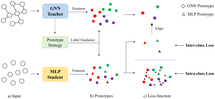
Figure 1: Overview of the proposed PGKD. The input is the whole graph for the GNN teacher but only the corresponding graph nodes for the MLP student. The circles mean the vectors for graph nodes and the same color denotes the same class. After getting the class prototypes, we design inter-class and intra-class loss to distill the graph structural information from the GNN teacher to the MLP student.

3 Methodology

3.1 Impact of Graph Structures on GNNs

Here we study the impact of graph structures (graph edges) on GNNs. Based on that, PGKD is subsequently derived. We first categorize the graph edges into intra-class and inter-class edges based on whether the connected nodes are from the same or different classes, respectively.

Intra-class Edges.

The propagation mechanisms in GNNs are the optimal solution of optimizing a feature fitting function with a graph Laplacian regularization term Zhu et al. (2021); Ma et al. (2021). The Laplacian regularization guides the smoothness of $\mathbf{H}$ over $\mathcal{G}$, where connected nodes share similar features. Therefore, the homophily property for nodes from the same class can be captured. As shown in Table 7, the average connected node distance for GNNs is much smaller than that in initial node features.

Inter-class Edges.

For inter-class edges, the nodes connected belong to different classes, which is known as heterophily. We define the class distance as the distance between class prototypes, and the class prototype is the prototypical vector for all nodes from the same class. The inter-class edges determine the pattern of class distances: for class $i,j,k$, if the inter-class edges between class $i,j$ are more than class $i,k$, then the class distance of $i,j$ would be smaller. From Table 8, we can infer that two classes would be closer if more inter-class edges exist between them in GNNs.

3.2 Prototype-Guided Knowledge Distillation

Since the impact of graph structures (i.e. graph edges) on GNNs has been studied, the next goal is to distill such graph structural information from GNNs to MLPs. In PGKD, we design two losses to mimic the impact of intra-class and inter-class edges via class prototypes. Figure 1 shows the overview of PGKD.

Prototype Strategy.

To get the class prototype, the key is to label all nodes. In the inductive scenario, we employ the corresponding ground-truth label $\mathbf{Y}^{L}$ of training data for both GNN teachers and MLP students. However, in transductive scenarios, applying the ground-truth label $\mathbf{Y}$ would lead to label leaking. Hence, we employ the predicted label of the GNN teacher to label the MLP nodes. After grouping the nodes via the labels, we define the class prototypes as the mean vectors of all nodes from the same class. Henceforth, we use $(\mathbf{P}^{t}_{1},...,\mathbf{P}^{t}_{K})$ and $(\mathbf{P}^{s}_{1},...,\mathbf{P}^{s}_{K})$ to denote the GNN and MLP class prototypes, respectively.

Intra-class Loss.

The intra-class edges in GNNs capture the homophily property for nodes from the same class. One intuitive idea is to draw closer for any two nodes from the same classes in the edge-free setting. However, this strategy has two drawbacks: 1) It is easily influenced by the outlines, viz. noisy points; and 2) A heavy computing as much as $O(n^{2})$ where $n$ denotes the quantity of a given class. In PGKD, the goal is to draw a selected node closer to its corresponding prototype. We design the intra-class loss analogous to InfoNCE van den Oord et al. (2018). For node $i$ and its given label $c_{i}$, the loss is calculated as follows:

$$\mu_{i}=[d_{1}(h_{i},\mathbf{P}^{s}_{1}),...,d_{1}(h_{i},\mathbf{P}^{s}_{K})]\vspace{-0.5em}$$ (3)

$$\mathcal{L}_{intra}=\Phi_{1}(\text{Softmax}(-\mu_{i}/\tau_{1}),c_{i}),\vspace{-0.5em}$$ (4)

where $\Phi_{1}$ denotes loss functions such as cross-entropy loss, $\tau_{1}$ denotes the temperature parameter, and $d_{1}$ denotes the distance function. The class prototypes are less sensitive to noisy points. Meanwhile, the computing cost is decreased into $O(n\times K)$ where $K\ll n$ typically.

Inter-class Loss.

The inter-class edges determine the pattern of class distances. The class prototypes would be closer if more inter-class edges connect these two classes. However, we cannot count the edges in an edge-free setting. One solution is to force the student to mimic the distance pattern of GNN teachers. Aligning the distances directly can not work, since the node representations from teacher and student lie in different semantic space. Therefore, we calculate the relative distance in PGKD. The loss to align GNN prototype $\mathbf{P}^{t}_{i}$ and MLP prototype $\mathbf{P}^{s}_{i}$ is calculated by:

$$\sigma^{t}_{i}=[d_{2}(\mathbf{P}^{t}_{i},\mathbf{P}^{t}_{1}),...,d_{2}(\mathbf{P}^{t}_{i},\mathbf{P}^{t}_{K})]\vspace{-0.5em}$$ (5)

$$\sigma^{s}_{i}=[d_{2}(\mathbf{P}^{s}_{i},\mathbf{P}^{s}_{1}),...,d_{2}(\mathbf{P}^{s}_{i},\mathbf{P}^{s}_{K})]\vspace{-0.5em}$$ (6)

$$\mathcal{L}_{inter}=\Phi_{2}(\text{Softmax}(\sigma^{s}_{i}/\tau_{2}),\text{Softmax}(\sigma^{t}_{i}/\tau_{2})),\vspace{-0.5em}$$ (7)

where $\Phi_{2}$ denotes the similarity function for two distributions such as KL-divergence, $\tau_{2}$ denotes the temperature parameter, and $d_{2}$ denotes the distance function.

Overall Target.

In PGKD, the overall loss function is:

$$\mathcal{L}=\mathcal{L}_{label}+\mathcal{L}_{kd}+\lambda_{1}\mathcal{L}_{intra}+\lambda_{2}\mathcal{L}_{inter},$$ (8)

where $\mathcal{L}_{label}$ and $\mathcal{L}_{kd}$ are the original loss for classification and vanilla logit-base KD loss, respectively. $\lambda_{1}$ and $\lambda_{2}$ are the hyperparameters. This way, the baseline GLNN is a special case of PGKD when both $\lambda_{1}$ and $\lambda_{2}$ are zeroed.

4 Experiments

This section presents an empirical study of PGKD on several popular graph benchmarks.

4.1 Datasets

To evaluate the performance of PGKD, we consider six popular benchmarks, including four homophilous graph datasets, namely, Cora Sen et al. (2008), Citeseer Sen et al. (2008), Pubmed Namata et al. (2012), and A-computer Shchur et al. (2018), and two heterophilous graph datasets, namely, Penn94 Lim et al. (2021) and Twitch-gamer Lim et al. (2021). Table 3 shows the dataset details. We split these datasets for train/validation/test following GLNN Zhang et al. (2022) for fair comparison. For the metric, we report the average accuracy on test data over five runs with different random seeds.

Datasets	#Nodes	#Edges	#Features	#Classes
Cora	2708	5429	1433	7
Citeseer	3327	4732	3703	6
A-computer	7650	119081	745	8
Pumbed	19717	44324	500	3
Penn94	41554	1362229	5	2
Twitch-gamer	168114	6797557	7	2

Table 3: Statistics of the benchmarks

4.2 Implementation

GNN Teacher.

To evaluate the ability on different backbones, we select four popular GNNs as the teacher model: GraphSAGE Hamilton et al. (2017), GAT Velickovic et al. (2017), GCN Kipf and Welling (2017) and APPNP Klicpera et al. (2019), and perform experiments under both transductive and inductive settings.

Baselines.

For baselines, we do not compare with the regularization methods since these methods utilize the graph edges as extra inputs. In real-world applications, these graph edges may be unavailable such as in federated graph learning. Therefore, we conduct all experiments in the edge-free setting. For fairness, we select the edge-free GLNN Zhang et al. (2022) as our baseline, which adapts vanilla logit-base KD from GNNs to MLPs.

Hyper-parameters.

We distill the two-layer GNN teacher to MLP student with two layers (on Cora, Citeseer, and A-computer) or three layers (on Pumbed, Penn94, and Twitch-gamer). For PGKD, we employ grid search to train the MLPs, where $\lambda_{1}$ is searched in $\{0.1,0.2,0.4\}$ and $\lambda_{2}$ in $\{0.05,0.1\}$. We set $\tau_{1}$ and $\tau_{2}$ as 1 and 10, respectively. The hidden state dimension is 128 for both GNNs and MLPs. On all the datasets, the MLPs are trained for 500 epochs with early stopping.

4.3 Main Results

Dataset	GNN Setting		GNN	GLNN	PGKD (Ours)	$\Delta$GLNN
Cora	SAGE	transductive	81.11$\pm$2.05	80.22$\pm$1.81	82.15$\pm$0.19	$\uparrow$ 1.93
		inductive	81.59$\pm$1.95	74.38$\pm$0.85	74.85$\pm$0.24	$\uparrow$ 0.47
Citeseer	SAGE	transductive	70.62$\pm$1.53	71.87$\pm$1.90	72.93$\pm$1.17	$\uparrow$ 1.06
		inductive	69.89$\pm$2.80	69.34$\pm$2.10	69.94$\pm$2.03	$\uparrow$ 0.60
A-computer	SAGE	transductive	82.70$\pm$0.69	82.84$\pm$1.04	83.42$\pm$0.39	$\uparrow$ 0.58
		inductive	83.12$\pm$0.88	80.94$\pm$0.83	81.78$\pm$0.50	$\uparrow$ 0.84
Penn94	GCN	transductive	82.08$\pm$0.40	81.08$\pm$0.50	81.51$\pm$0.48	$\uparrow$ 0.43
		inductive	81.95$\pm$0.52	71.67$\pm$0.52	72.18$\pm$0.50	$\uparrow$ 0.51
Pubmed	GCN	transductive	76.44$\pm$2.44	76.66$\pm$3.34	77.02$\pm$2.85	$\uparrow$ 0.36
		inductive	75.68$\pm$2.80	73.95$\pm$5.56	76.35$\pm$2.21	$\uparrow$ 1.86
Twitch-gamer	GCN	transductive	62.58$\pm$0.19	60.07$\pm$0.16	60.56$\pm$0.07	$\uparrow$ 0.49
		inductive	62.34$\pm$0.44	59.57$\pm$0.30	60.01$\pm$0.42	$\uparrow$ 0.44

Table 4: Experiment results for PGKD on several benchmarks under transductive and inductive settings. We report the average test accuracy (%) and the standard deviation over five runs for each dataset. PGKD outperforms GLNN with higher average score and lower standard deviation.

We conduct the experiments on six benchmarks and select SAGE as GNN teachers for small datasets (Cora, Citeseer and A-computer) and GCN for large datasets (Penn94, Pubmed and Twitch-gamer). Meanwhile, we reproduce GLNN from its official codes. Table 4 reports the accuracy results. Some observations are in place:

1. PKGD outperforms GLNN on all six benchmarks with higher average scores under both transductive and inductive settings, thus demonstrating the effectiveness of PGKD in capturing graph structural information for the MLPs. In particular, PGKD achieves 76.35% on Pubmed under inductive setting, which is 1.86% higher than GLNN. PKGD can even outperform GNN teachers on some datasets (Citeseer and Pubmed).

2. The standard deviations of PGKD are smaller than GLNN for almost all datasets, showing the stability and robustness of PGKD. For instance, PGKD gets 0.39% on A-computer under transductive setting, which is approximately 3$\times$ smaller than the 1.04% of GLNN.

4.4 Ablation Studies

To better understand PGKD, we conduct ablation experiments on intra-class loss and inter-class loss. Without loss of generality, we select SAGE, GAT, GCN, APPNP as GNN teachers and compare the performance on Citeseer under inductive setting and Cora under transductive setting.

Table 5&6 show the experiment results. From the tables, we find that the performance drops when either intra-class loss or inter-class loss is removed, indicating that both intra-class information and inter-class information are vital. In general, removing the intra-class loss would lead to a larger drop than the inter-class loss under the transductive setting, but a smaller drop under the inductive setting. Moreover, it is quite interesting to find that PGKD with one loss exclusively would perform worse than GLNN, but is better than GLNN with two losses together. For example, PGKD gets 68.62% and 68.23% (APPNP as GNN teacher) on Citeseer with one loss exclusively, which are lower than 69.23% of GLNN. However, PGKD would get a higher 69.78% than GLNN with two losses. Adopting SAGE as the GNN teacher on Citeseer also leads to a similar situation. Such phenomenon indicates that simultaneously capturing both intra-class information and inter-class information is crucial for the MLP training.

Model	SAGE	GAT	GCN	APPNP
GNN	69.89$\pm$2.83	71.69$\pm$2.90	70.83$\pm$3.12	72.93$\pm$2.11
GLNN	69.34$\pm$2.10	69.12$\pm$3.83	69.01$\pm$2.92	69.23$\pm$1.74
PGKD	69.94$\pm$2.03	69.89$\pm$4.51	70.00$\pm$2.00	69.78$\pm$1.59
-$\mathcal{L}_{intra}$	69.01$\pm$1.76	68.51$\pm$5.03	69.28$\pm$2.28	68.62$\pm$1.77
-$\mathcal{L}_{inter}$	68.62$\pm$2.87	69.17$\pm$3.62	69.12$\pm$1.98	68.23$\pm$2.01

Table 5: The ablation accuracy (%) on Citeseer dataset for several GNN teachers under inductive setting. We report the results for five runs.

Model	SAGE	GAT	GCN	APPNP
GNN	81.11$\pm$2.05	81.81$\pm$1.28	82.24$\pm$0.59	83.26$\pm$0.87
GLNN	80.22$\pm$1.81	79.92$\pm$1.00	81.43$\pm$0.18	79.40$\pm$1.34
PGKD	82.15$\pm$0.19	81.65$\pm$1.47	82.39$\pm$0.64	82.59$\pm$1.11
-$\mathcal{L}_{intra}$	80.83$\pm$1.26	80.21$\pm$1.10	81.12$\pm$0.92	79.55$\pm$1.04
-$\mathcal{L}_{inter}$	81.17$\pm$1.62	81.98$\pm$1.04	81.91$\pm$0.54	82.79$\pm$0.86

Table 6: The ablation results (%) on Cora dataset for several GNN teachers under transductive setting. We report the results for five runs.

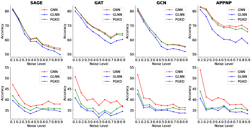
Figure 2: The performance of GNN teacher, distilled MLP students via GLNN and PKGD when adding different noise to the initial node features. For GNN teachers, we select SAGE, GAT, GCN and APPNP, respectively. Upper: Cora dataset and transductive setting. Lower: Pubmed dataset and inductive setting.

5 Analysis and Discussion

We further explore the ability to capture graph structural information as well as the robustness of the proposed PGKD. We also visualize the distributions of node representations for deeper insights.

5.1 Can PGKD distill the Impact of Graph Edges?

As mentioned in Section 3.1, the intra-class edges guarantee the homophily for nodes from the same class, while the inter-class edges determine the pattern of distances among class prototypes.

We adopt SAGE as the GNN teacher and perform experiments under a transductive setting, and then calculate the average L2 distance for the features of connected nodes in the graph. Table 7 shows the average distance of initial node features and node features from GNN teacher (SAGE), GLNN, and PGKD. The distance of the GNN teacher is the shortest due to the information aggregation operations along graph edges. Meanwhile, the distance for GLNN is much longer due to the weak awareness of such graph structural information. PGKD gets shorter distances than GLNN, showing a great ability to capture intra-class graph structural information. In particular, PGKD gets a L2 distance of 0.82 on Citeseer, which is shorter than 3.10 from the GLNN.

Dataset	Input	GNN	GLNN	PGKD
Cora	4.40	1.95	3.02	2.47
Citeseer	5.66	1.40	3.10	0.82
A-computer	17.63	2.35	7.14	4.76

Table 7: Average L2 distance for the features of connected nodes on different datasets.

Dataset	GNN	GLNN	PGKD
Cora	-0.94	-0.88	-0.92
Citeseer	-0.71	-0.62	-0.67
A-computer	-0.75	-0.60	-0.77

Table 8: Spearman correlation $\rho$ between class distances and inter-class edges quantity. $\rho\to-1$ indicates more negatively correlated for two variables.

The inter-class edges determine the pattern of distances among class prototypes. Specifically, the prototypes of two classes would be closer with more inter-edges connecting them in GNNs. We take statistics on the class distances (defined as L2 distances among class prototypes) and quantity of corresponding inter-class edges. For qualitative analysis, we calculate the Spearman correlation. From Table 8, the GNN teacher has a low Spearman correlation, whereas GLNN shows a relatively high value. Meanwhile, the proposed PGKD, thanks to the intra-class loss, can better capture the intra-class graph structural information and exhibits a much lower correlation.

5.2 Is PGKD Robust to Noisy Node Features?

To analyze the robustness of PGKD on node noise, we further evaluate the performance after adding Gaussian noise of different levels to initial node features $X$. Specifically, we replace $X$ with $(1-\alpha)X+\alpha\epsilon$, where $\epsilon$ denotes the isotropic Gaussian noise independent from $X$, and $\alpha\in[0,1]$ controls the noise level. A larger $\alpha$ means a stronger noise. Figure 2 shows the performance of GNN, GLNN, and PGKD under different noise levels. On both Cora and Pumbed, PGKD outperforms GLNN consistently as the noise level ranges from 0.1 to 0.9. Particularly, PGKD could get better results than GAT and APPNP on Pumbed with $\alpha=0.9$. These show that PGKD is more robust than GLNN with respect to noisy input node features due to its ability to capture graph structural information.

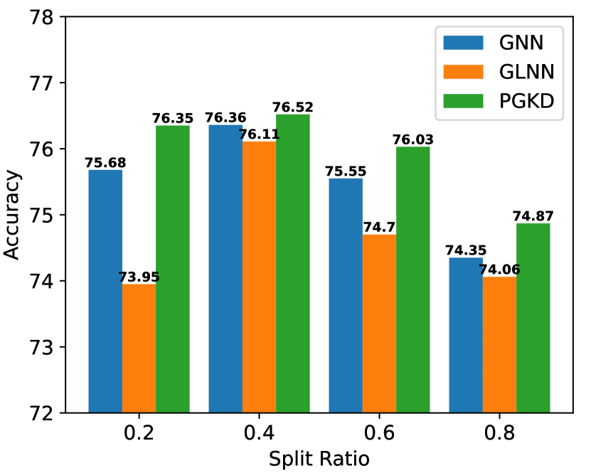
Figure 3: The performance of GNN teacher, distilled MLP students via GLNN and PKGD under inductive setting with different split ratio. We select GCN as GNN teacher and perform experiments on Pubmed dataset.

5.3 Impact of Inductive Split Ratio

To evaluate the ability for less observed data under inductive setting, we conduct the experiments under different split ratios, defined as the ratio $|\mathcal{V}^{U}_{ind}|/|\mathcal{V}^{U}|$. A larger split ratio means less observed unlabeled data during training and more inductive unlabeled data for test (cf. Section 2). As shown in Figure 3, the performance of the GNN teacher is not monotonically decreasing since the way to split graph (i.e. the edges to remove) is also vital as the number of nodes for training. PGKD outperforms GLNN and GNN under all split ratios. Also, the performance of PGKD is more stable than GLNN. This proves that PKGD, explicitly capturing the graph structural information, is robust and effective under different inductive split ratios.

5.4 Impact of MLP Setting

#L	#H	Params	MLP	GLNN	PGKD	$\Delta$GLNN
2	64	0.09M	53.40	73.30	74.00	$\uparrow$0.70
2	128	0.18M	59.48	71.66	74.71	$\uparrow$3.05
3	128	0.20M	54.33	73.07	74.24	$\uparrow$1.17
2	512	0.73M	56.21	73.54	74.47	$\uparrow$0.92
3	512	1.00M	54.57	72.83	74.00	$\uparrow$1.17

Table 9: Comparisons for vanilla MLP, distilled MLP students via GLNN and PGKD with different MLP settings on Cora under inductive setting. We report the average test accuracy (%). #L denotes the layers and #H denotes dimension of hidden state.

We further conduct experiments using different MLP settings. The GNN teacher is a two-layer GCN with 0.18M parameters and gets an accuracy of 83.37% on Cora dataset. As shown in Table 9, the vanilla MLP shows an overfitting trend when the number of parameters increases, while the PGKD does not. Meanwhile, PGKD gets the highest results under all settings and shows consistent improvement over GLNN. In particular, GLNN gets a score of 74.71% (#L=2, #H=128), which is 3.05% higher than GLNN. Such findings indicate that PGKD is more robust and effective in different MLP settings.

5.5 Node Representation Distribution

We visualize the distribution of node representations from GNNs and MLPs (vanilla MLPs without KD, MLPs from GLNN, and MLPs from PGKD) via t-SNE van der Maaten and Hinton (2008). We select the GAT as the GNN teachers. Figure 4 shows the results on Cora and Citeseer under transductive setting. Due to the message passing architecture, the node representations in the same class from GNNs are much more gathered than vanilla MLPs. PGKD captures such graph information via intra-class loss, while vanilla MLPs and MLPs from GLNN lack such capability. The same-class features from both GLNN and vanilla MLP are slightly dispersed, while the features from PGKD are more clustered inside a class and separable between classes. Moreover, PGKD can learn better class prototype distributions. Specifically, in the GNN representations on Cora, the dark green and purple classes are far from each other. PGKD captures such a behavior well, where GLNN fails.

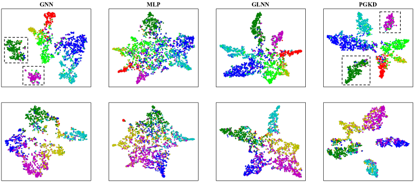
Figure 4: The distribution of node representations for GNN teacher, vanilla MLP, and distilled MLPs from GLNN and PKGD. Upper: Cora dataset. Lower: Citeseer dataset.

6 Related Work

6.1 Distill GNNs to MLPs

Knowledge Distillation (KD) is among the mainstream approaches to transferring knowledge from GNNs to MLPs. The key insight is to learn a student model by mimicking the behaviors of the teacher model. GLNN Zhang et al. (2022) utilizes the vanilla logit-based KD Hinton et al. (2015), which is edge-free but fails to capture the graph structural information. To address this issue, one way is to process graph edges into extra inputs for MLPs, such as the adjacent matrix Chen et al. (2022) or the node positions Tian et al. (2022). Another line is to treat graph structural information as a regularization term, where the nodes connected by edges should be closer Wu et al. (2022); Hu et al. (2021). Nonetheless, graph structure may be unavailable for some scenarios, e.g., in federated graph learning.

In this work, we show it is possible to effectively distill the graph structural knowledge from GNNs to MLPs under an edge-free setting.

6.2 Prototype in GNNs

Prototypical Networks Snell et al. (2017) have been widely applied in few-shot learning and metric learning on classification tasks Huang and Zitnik (2020). The basic idea is that there exists an embedding in which points cluster around a single prototype representation for each class. In GNNs, class prototypes are widely employed for few-shot classification Satorras and Estrach (2018); Yao et al. (2020), zero-shot classification Wang et al. (2021), graph matching Wang et al. (2020), and graph explanation Shin et al. (2022); Ying et al. (2019). The class prototypes are usually defined as simple as mean vectors.

In this work, we employ the class prototypes and design extra losses for MLP students via prototypes, aiming to capture the graph structural information from GNN teachers. To our best knowledge, this is the first use of prototypes for GNN-to-MLP distillation.

7 Conclusion

A novel PGKD scheme has been proposed to distill the knowledge from high-accuracy GNNs to low-latency MLPs, wherein the distillation process is edge-free and the learned MLP students are structure-aware. Specifically, we analyze the impact of graph structure (graph edges) on GNNs and categorize them into intra-class and inter-class edges. Two corresponding losses via class prototypes are designed to transfer the graph structural knowledge from GNNs to MLPs. Experiments on popular benchmarks demonstrate the effectiveness of PGKD. Additionally, we show PGKD is robust to noisy node features, and performs well under different training settings.

For our future work, PGKD will be generalized to other graph tasks beyond node classification. Another interesting direction will be to generate prototypes utilizing node representations rather than class labels.

Limitations

In PGKD, we adopt the class prototypes to capture graph structural information for MLPs in an edge-free setting. Subsequently, PGKD requires slightly more computing cost compared to the baseline GLNN. Meanwhile, the gap between the MLP learned by PGKD and its teacher GNN under the inductive setting is larger than that under the transductive setting, especially on Cora and Penn94 datasets. More effort to improve the performance under the inductive setting is required underway.

References

- Chen et al. (2022) Jie Chen, Shouzhen Chen, Mingyuan Bai, Junbin Gao, Junping Zhang, and Jian Pu. 2022. SA-MLP: distilling graph knowledge from gnns into structure-aware MLP. CoRR, abs/2210.09609.
- Chopra et al. (2005) Sumit Chopra, Raia Hadsell, and Yann LeCun. 2005. Learning a similarity metric discriminatively, with application to face verification. In 2005 IEEE Computer Society Conference on Computer Vision and Pattern Recognition (CVPR 2005), 20-26 June 2005, San Diego, CA, USA, pages 539–546. IEEE Computer Society.
- Hamilton et al. (2017) William L. Hamilton, Zhitao Ying, and Jure Leskovec. 2017. Inductive representation learning on large graphs. In Advances in Neural Information Processing Systems 30: Annual Conference on Neural Information Processing Systems 2017, December 4-9, 2017, Long Beach, CA, USA, pages 1024–1034.
- Hinton et al. (2015) Geoffrey E. Hinton, Oriol Vinyals, and Jeffrey Dean. 2015. Distilling the knowledge in a neural network. CoRR, abs/1503.02531.
- Hu et al. (2021) Yang Hu, Haoxuan You, Zhecan Wang, Zhicheng Wang, Erjin Zhou, and Yue Gao. 2021. Graph-mlp: Node classification without message passing in graph. CoRR, abs/2106.04051.
- Huang and Zitnik (2020) Kexin Huang and Marinka Zitnik. 2020. Graph meta learning via local subgraphs. In Advances in Neural Information Processing Systems 33: Annual Conference on Neural Information Processing Systems 2020, NeurIPS 2020, December 6-12, 2020, virtual.
- Jia et al. (2020) Zhihao Jia, Sina Lin, Rex Ying, Jiaxuan You, Jure Leskovec, and Alex Aiken. 2020. Redundancy-free computation for graph neural networks. In KDD ’20: The 26th ACM SIGKDD Conference on Knowledge Discovery and Data Mining, Virtual Event, CA, USA, August 23-27, 2020, pages 997–1005. ACM.
- Kipf and Welling (2017) Thomas N. Kipf and Max Welling. 2017. Semi-supervised classification with graph convolutional networks. In 5th International Conference on Learning Representations, ICLR 2017, Toulon, France, April 24-26, 2017, Conference Track Proceedings. OpenReview.net.
- Klicpera et al. (2019) Johannes Klicpera, Aleksandar Bojchevski, and Stephan Günnemann. 2019. Predict then propagate: Graph neural networks meet personalized pagerank. In 7th International Conference on Learning Representations, ICLR 2019, New Orleans, LA, USA, May 6-9, 2019. OpenReview.net.
- Lim et al. (2021) Derek Lim, Felix Hohne, Xiuyu Li, Sijia Linda Huang, Vaishnavi Gupta, Omkar Bhalerao, and Ser-Nam Lim. 2021. Large scale learning on non-homophilous graphs: New benchmarks and strong simple methods. In Advances in Neural Information Processing Systems 34: Annual Conference on Neural Information Processing Systems 2021, NeurIPS 2021, December 6-14, 2021, virtual, pages 20887–20902.
- Liu and Yu (2022) Rui Liu and Han Yu. 2022. Federated graph neural networks: Overview, techniques and challenges. CoRR, abs/2202.07256.
- Ma et al. (2021) Yao Ma, Xiaorui Liu, Tong Zhao, Yozen Liu, Jiliang Tang, and Neil Shah. 2021. A unified view on graph neural networks as graph signal denoising. In CIKM ’21: The 30th ACM International Conference on Information and Knowledge Management, Virtual Event, Queensland, Australia, November 1 - 5, 2021, pages 1202–1211. ACM.
- Namata et al. (2012) Galileo Namata, Ben London, Lise Getoor, and Bert Huang. 2012. Query-driven active surveying for collective classification.
- Satorras and Estrach (2018) Victor Garcia Satorras and Joan Bruna Estrach. 2018. Few-shot learning with graph neural networks. In 6th International Conference on Learning Representations, ICLR 2018, Vancouver, BC, Canada, April 30 - May 3, 2018, Conference Track Proceedings. OpenReview.net.
- Sen et al. (2008) Prithviraj Sen, Galileo Namata, Mustafa Bilgic, Lise Getoor, Brian Gallagher, and Tina Eliassi-Rad. 2008. Collective classification in network data. AI Mag., 29(3):93–106.
- Shchur et al. (2018) Oleksandr Shchur, Maximilian Mumme, Aleksandar Bojchevski, and Stephan Günnemann. 2018. Pitfalls of graph neural network evaluation. CoRR, abs/1811.05868.
- Shin et al. (2022) Yong-Min Shin, Sun-Woo Kim, and Won-Yong Shin. 2022. PAGE: prototype-based model-level explanations for graph neural networks. CoRR, abs/2210.17159.
- Snell et al. (2017) Jake Snell, Kevin Swersky, and Richard S. Zemel. 2017. Prototypical networks for few-shot learning. In Advances in Neural Information Processing Systems 30: Annual Conference on Neural Information Processing Systems 2017, December 4-9, 2017, Long Beach, CA, USA, pages 4077–4087.
- Tian et al. (2022) Yijun Tian, Chuxu Zhang, Zhichun Guo, Xiangliang Zhang, and Nitesh V. Chawla. 2022. NOSMOG: learning noise-robust and structure-aware mlps on graphs. CoRR, abs/2208.10010.
- van den Oord et al. (2018) Aäron van den Oord, Yazhe Li, and Oriol Vinyals. 2018. Representation learning with contrastive predictive coding. CoRR, abs/1807.03748.
- van der Maaten and Hinton (2008) Laurens van der Maaten and Geoffrey Hinton. 2008. Visualizing data using t-sne. Journal of Machine Learning Research, 9(86):2579–2605.
- Velickovic et al. (2017) Petar Velickovic, Guillem Cucurull, Arantxa Casanova, Adriana Romero, Pietro Liò, and Yoshua Bengio. 2017. Graph attention networks. CoRR, abs/1710.10903.
- Wang et al. (2021) Zheng Wang, Jialong Wang, Yuchen Guo, and Zhiguo Gong. 2021. Zero-shot node classification with decomposed graph prototype network. In KDD ’21: The 27th ACM SIGKDD Conference on Knowledge Discovery and Data Mining, Virtual Event, Singapore, August 14-18, 2021, pages 1769–1779. ACM.
- Wang et al. (2020) Zijian Wang, Yadan Luo, Zi Huang, and Mahsa Baktashmotlagh. 2020. Prototype-matching graph network for heterogeneous domain adaptation. In MM ’20: The 28th ACM International Conference on Multimedia, Virtual Event / Seattle, WA, USA, October 12-16, 2020, pages 2104–2112. ACM.
- Wu et al. (2022) Lirong Wu, Jun Xia, Haitao Lin, Zhangyang Gao, Zicheng Liu, Guojiang Zhao, and Stan Z. Li. 2022. Teaching yourself: Graph self-distillation on neighborhood for node classification. CoRR, abs/2210.02097.
- Yao et al. (2020) Huaxiu Yao, Chuxu Zhang, Ying Wei, Meng Jiang, Suhang Wang, Junzhou Huang, Nitesh V. Chawla, and Zhenhui Li. 2020. Graph few-shot learning via knowledge transfer. In The Thirty-Fourth AAAI Conference on Artificial Intelligence, AAAI 2020, The Thirty-Second Innovative Applications of Artificial Intelligence Conference, IAAI 2020, The Tenth AAAI Symposium on Educational Advances in Artificial Intelligence, EAAI 2020, New York, NY, USA, February 7-12, 2020, pages 6656–6663. AAAI Press.
- Ying et al. (2019) Zhitao Ying, Dylan Bourgeois, Jiaxuan You, Marinka Zitnik, and Jure Leskovec. 2019. Gnnexplainer: Generating explanations for graph neural networks. In Advances in Neural Information Processing Systems 32: Annual Conference on Neural Information Processing Systems 2019, NeurIPS 2019, December 8-14, 2019, Vancouver, BC, Canada, pages 9240–9251.
- Zhang et al. (2022) Shichang Zhang, Yozen Liu, Yizhou Sun, and Neil Shah. 2022. Graph-less neural networks: Teaching old mlps new tricks via distillation. In The Tenth International Conference on Learning Representations, ICLR 2022, Virtual Event, April 25-29, 2022. OpenReview.net.
- Zhu et al. (2021) Meiqi Zhu, Xiao Wang, Chuan Shi, Houye Ji, and Peng Cui. 2021. Interpreting and unifying graph neural networks with an optimization framework. In WWW ’21: The Web Conference 2021, Virtual Event / Ljubljana, Slovenia, April 19-23, 2021, pages 1215–1226. ACM / IW3C2.