Associated Random Neural Networks for Collective Classification of Nodes in Botnet Attacks

Abstract

Botnet attacks are a major threat to networked systems because of their ability to turn the network nodes that they compromise into additional attackers, leading to the spread of high volume attacks over long periods. The detection of such Botnets is complicated by the fact that multiple network IP addresses will be simultaneously compromised, so that Collective Classification of compromised nodes, in addition to the already available traditional methods that focus on individual nodes, can be useful. Thus this work introduces a collective Botnet attack classification technique that operates on traffic from a $n$-node IP network, with a novel Associated Random Neural Network (ARNN) that identifies the nodes which are compromised. The ARNN is a recurrent architecture that incorporates two mutually associated, interconnected and architecturally identical $n$-neuron random neural networks, that act simultneously as mutual critics to reach the decision regarding which of $n$ nodes have been compromised. A novel gradient learning descent algorithm is presented for the ARNN, and is shown to operate effectively both with conventional off-line training from prior data, and with on-line incremental training without prior off-line learning. Real data from a $107$ node packet network is used with over $700,000$ packets to evaluate the ARNN, showing that it provides accurate predictions. Comparisons with other well-known state of the art methods using the same learning and testing datasets, show that the ARNN offers significantly better performance.

1 Introduction

Many classification problems, such as identifying a given individual’s face in a large dataset of face images of people [1], associate a binary label to data items [2]. This is also the usual case for network attack detection from traffic data [3] that attemps to determine whether a given network node has been compromised by an attack [4]. Such problems are often solved with Machine Learning (ML) algorithms that learn off-line from one or more datasets that contain the ground-truth data. The trained ML algorithm can then be tested on datasets that have not been used for learning, and then used online with previously unseen or new data. Typically, the online usage of such attack detection algorithms is carried out “one node at a time”, i.e. as an individual classification problem for a specific node that may be concerned by possible attacks [5, 6].

When we need to classify each individual node in a set $V=\{v_{1},~{}...~{},v_{n}\}$ of interconnected nodes in a network as being “compromised” or uncompromised (i.e., “safe”) we obviously face with a Binary Individual Classification Problem for each of the $n$ nodes. However, when the attacking entity is a Botnet which induces a compromised node to attack several other nodes with which it is able to directly communicate, then we are faced with a Collective Binary Classification Problem where the classification of the distinct nodes is correlated, even though we cannot be sure that a compromised node has sufficient bandwidth or processing capacity to actually compromise other nodes.

Indeed let $A=[A_{ij}]_{n\times n}$ be the (deterministic) adjacency matrix where $A_{ij}=1$ indicates that node $v_{i}$ has opened a connection to node $v_{j}$ and therefore can send packet traffic to it, while $A_{ij}=0$ indicates that node $v_{i}$ is unable to send packets to node $v_{j}$. Then during a Botnet attack, nodes that can receive traffic from compromised nodes are themselves likely to become compromised, and to become in turn attackers against other nodes, so that one needs to classify nodes by taking account both the local atack traffic at each node, and their patterns of communication between nodes.

Collective (also known as “relational”) classification problems have been widely studied [7, 8] using a variety of techniques linked to ML. As indicated in the literature [9], collective classification may use a collection of local conditional classifiers which classify an individual’s label conditionally on the label value of others, and then fuses the overall sets of outputs, or may try to solves the problem either as a global optimization or a global relaxation problem [10, 11], with the global approach being often computationally more costly.

Botnet attack detection has been discussed in numerous papers, mainly using single node attack detection techniques [12, 13, 14] which can identify individually comprimised nodes, except for some studies that analyze relations between nodes to detect the existence or spread of a Botnet [15, 16, 17].

Thus in this paper we address the Collective Classification problem of detecting all the nodes in a given network which have been compromised by a Botnet. In particular, we introduce a ML method that combines supervised learning by a novel Random Neural Network [18] architecture – which we call the Associated Random Neural Network (ARNN) – that learns from a sample taken from the traffic flowing among a set of network nodes, to classify them as being either compromised by a Botnet, or as non-compromised.

The Random Neural Network is a bio-inspired spiking Neural Network that has a convenient mathematical solution, and has been applied by numerous authors, including [19, 20, 21, 22, 23, 24, 25, 26, 27, 28, 29, 30, 31, 32, 33, 34, 35, 36, 37, 38, 39], in diverse problems that can be addressed with ML such as video compression, tumor recognition from MRI images, video quality evaluation, smart building climate management, enhanced reality, voice quality evaluation over the internet, wireless channel modulation, climate control in buildings, the detection of network viruses and other cyberattacks.

In the case of Botnet detection, the ARNN is trained off-line with data that is certified as containing Botnet attacks, and with data that is attack free, and the trained ARNN is then used online to monitor a network’s traffic to collectively classfy which nodes – if any – are compromised by a Botnet.

In the sequel, Section 2 surveys previous research on Botnet attacks. In Section 3 the proposed ARNN is described; to improve readability its gradient learning algorithm is detailed separately in A.

Section 4 presents the experimental work based on a large MIRAI Botnet dataset involving $107$ network nodes and over $760,000$ packets [40] that is used for training and evaluating the proposed method. The evaluation of the ARNN using this dataset is detailed in Section 5, where we have also compared our results with other well known ML methods. Finally, conclusions and suggestions for further work are presented in Section 6.

2 Recent Work on Botnet Attack Detection

In networked systems the cost of not meeting security requirements can be very high [41, 42, 43], hence much effort has been devoted to developing techniques that detect attacks against network components such as hosts, servers, routers, switches, IoT devices, mobile devices and various network applications.

Botnet attacks are particularly harmful, since they induce their victims to become sources of further attacks against third parties [44, 45, 46]. Recent Botnet reports include the 2016 MIRAI attack [47], and the MERIS type attacks from 2021 and 2022 that can generate some $46$ million requests per second, lasting more than $60$ minutes, exploiting over $5,000$ source IP addresses as Bots from over $130$ countries [48, 49], which is a similar rate of requests as all the Wikimedia daily requests made in ten seconds. Another MERIS attack generated $17.2$ million requests per second against a commercial web site, and such attacks have been observed to target some $50$ web sites per day, with over $100$ Distributed Denial of Service (DDoS) attacks, of which one third appear to occur in China, and $13\%$ in the USA, involving a number of Bots sometimes ranging between $30,000$ up to $250,000$.

Botnet attack detection techniques typically examine incoming traffic streams and identify sub-streams that are benign or “normal”, and those that may contain attacks [50, 51, 52], and often classify attacks into “types” [53] based on signatures [54, 55] that exploit prior knowledge about attack patterns. In addition, false alarms should also be minimized so that useful network traffic is not eliminated by mistake. However, such methods can also be overwhelmed by attack generators [56] that have been designed to adaptively modify their behaviour.

Defense techniques for Botnets based on the smart location of counter-attacks by “white hat” worm launchers have also been suggested [57, 58], while refined deep learning (DL) techniques have been investigated to recognize constantly evolving Botnet traffic [59], and transfer learning can improve detection accuracy, without concatenating large datasets having different characteristics [60].

Recent work has also created a taxonomy of Botnet communication patterns including encryption and hiding [61] with some authors examining how Internet Service Providers (ISP) can participate collectively to mitigate their effect [62]. Other work suggests that traditional Botnet detection techniques in the Internet are not well adapted to emerging applications such as the IoT [63], some studies have addressed Botnet apps in specific operating system contexts such as Android [64] or Botnet detection for specific applications such as Peer to Peer Systems (P2P) [65], or Vehicular Networks for which specific detection and protection mechanisms are suggested [66].

Some recent research has focused on the manner in which Botnet variability can be reflected in intrusion detection software that is designed for a given host [67]. Universal sets of features that may be applicable to attack detection [68] have also been suggested, and detection techniques for specific types of Botnets such as the ones based on the Domain Generation Algorithm [69] have been proposed.

Most of the previous literature on Botnets, as well as our recent work, has focused on single node detection with off-line learning. We developed detection techniques for Distributed Denial of Service (DDoS) attacks using gradient descent learning with the RNN [4, 70], because Botnets often use DDoS as the means of bringing down their victims. The system-level remedial actions that should be taken after an attack is detected [71] were also analyzed. To avoid learning all possible types of attack patterns, an auto-associative approach based on Deep Learning of ”normal“ patterns with a dense multi-layer RNN [72] was developed to detect malicious attacks by identifying deviations from normal traffic [73, 74, 75]. It was also shown that a single trained auto-associative dense RNN can provide detection of multiple types of attacks (i.e. not just Botnets) [76], and that learning can be partially conducted on-line, with less need for long and computationally costly off-line training [6].

2.1 Approach Developed in this Paper

While it is possible to accurately detect malicious attacks by processing traffic at a given node, it is difficult to certify that the detected attack is indeed a Botnet by observing a single node since Botnets are based on the propagation of attack patterns through multiple nodes. Furthermore, many attack detectors detect anomalies in the incoming traffic rather that pointing to a specific attack [76]. Thus the present paper develops a Collective Classification approach to secifically address the Botnet detection problem in the following manner:

1. A finite set of $n$ interconnected network IP (Internet Protocol) addresses is considered,

2. Some of these addresses are equipped with a Local Attack Detector (LAD), so that a local evaluation is available at some of the nodes about whether they are being attacked. Note that the fact that a node is attacked does not necessarily imply that it has been compromised,

3. A specific neural network architecture, the Associated RNN (ARNN) with $2n$ neurons, is designed to deduce which (if any) of the IP addresses have been compromised by Botnet(s), using the available decisions from the LADs regarding individual nodes. The ARNN is trained, using the algorithm detailed in A, on a small subset of data taken from a large open access Botnet dataset [40] containing over $760,000$ packets exchanged among $107$ IP (Internet Protocol) addresses.

4. Then using the remaining large dataset (not used for training) we determine which of the $107$ IP addresses have been compromised and become Botnet attackers, resulting in a high level of accuracy regarding which IP addresses are compromised.

5. Two other well established ML methods are also used to identify which of the $107$ nodes have been compromised. The results show that the ARNN provides significantly better accuracy concerning both True Positives and True Negatives.

3 The ARNN Decision System

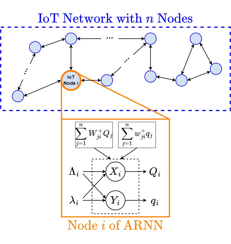
Figure 1: A schematic diagram of the $2n$-neuron ARNN that carries out a Collective Classification of the compromised nodes (if any) for a $n$-node IoT network denoted $V=\{v_{1},~{}...~{},v_{n}\}$. The ARNN has two neurons $X_{i}$ and $Y_{i}$ that represent opposite views for each network node $v_{i}$: $X_{i}$ indicates that $v_{i}$ is compromised, while $Y_{i}$ indicates that $v_{i}$ is not compromised. The corresponding numerical decision variables are $Q_{i},~{}q_{i}\in[0,1]$, where $Q_{i}$ is the probability that $X_{i}$ is excited and $q_{i}$ is the probability that $Y_{i}$ is excited. $X_{i}$ has an excitatory connection $W^{+}_{ij}$ to each other neuron $X_{j}$ and an inhibitory connection $W^{-}_{ij}$ to all other $Y_{j}$ neurons, and $Y_{i}$ has an excitatory connection $w^{+}_{ij}$ to each other neuron $Y_{j}$ and an inhibitory connection $w^{-}_{ij}$ to all other $X_{j}$ neurons. A neuron does not excite or inhibit its own self. Thus inside the ARNN, the neurons of type $X$ excite other neurons of type $X$ and inhibit all neurons of type $Y$, and vice-versa for the neurons of type $Y$. The ARNN is “self-critical” in the sense that neurons of type $X$ try to supress the neurons of type $Y$, and vice-versa. $\Lambda_{i}$ represents the output from the LAD (local attack detector) at node $v_{i}$ stating that $v_{i}$ has been compromised while $\lambda_{i}$ represents the LAD output at node $v_{i}$ stating that it has not been compromised. $\Lambda_{i},~{}\lambda_{i}$ act as an excitatory and inhibitory external input, respectively, for $X_{i}$, while they act as an inhibitory, excitatory input for $Y_{i}$.

The decision system presented in this paper, the “self-critical” ARNN with $2n$ neurons, is shown schematically in Figure 1. The ARNN carries out a Collective Classification of the compromised nodes (if any) for a $n$-node IP network denoted $V=\{v_{1},~{}...~{},v_{n}\}$. For each network node $v_{i}$, the ARNN has two neurons $X_{i}$ and $Y_{i}$ that represent opposite views. $X_{i}$ indicates that $v_{i}$ is compromised, while $Y_{i}$ indicates that $v_{i}$ is not compromised. Their corresponding numerical decision variables are $Q_{i},~{}q_{i}\in[0,1]$, where $Q_{i}$ is the probability that $X_{i}$ is excited and $q_{i}$ is the probability that $Y_{i}$ is excited. $X_{i}$ has an excitatory connection $W^{+}_{ij}$ to every other neuron $X_{j}$ and an inhibitory connection $W^{-}_{ij}$ to all $Y_{j}$ neurons, and $Y_{i}$ has an excitatory connection $w^{+}_{ij}$ to every other neuron $Y_{j}$ and an inhibitory connection $w^{-}_{ij}$ to all $X_{j}$ neurons. None of the neuron can directly excite or inhibit themselves. Thus inside the ARNN, the neurons of type $X$ excite other neurons of type $X$ and inhibit all neurons of type $Y$, and vice-versa for the neurons of type $Y$. The ARNN is “self-critical” in the sense that neurons of type $X$ try to supress the neurons of type $Y$, and vice-versa. $\Lambda_{i}$, is a non-negative real number that represents the output from the LAD (local attack detector) at $v_{i}$ stating that $v_{i}$ has been compromised while $\lambda_{i}$ represents the LAD output at node $v_{i}$ stating that it has not been compromised. $\Lambda_{i},~{}\lambda_{i}$ can be chosen from the corresponding probabilities outputted from the LADs acting as excitatory and inhibitory external input, respectively, for each $X_{i}$, while they have the opposite effect as inhibitory and excitatory input for $Y_{i}$, respectively.

The two neurons $X_{i}$ and $Y_{i}$ have internal states $K_{i}(t)\geq 0$ and $k_{i}(t)\geq 0$, respectively. If its internal state $K_{i}(t)$ is strictly positive, then the RNN neuron $X_{i}$ will fire spikes at exponentially distributed successive intervals, sending excitatory and/or inhibitory spikes at rates $W^{+}_{ij},~{}W^{-}_{ij}\geq 0$ to the other neurons in the ARNN. Similarly when $k_{i}(t)>0$ neuron $Y_{i}$ will fire spikes at rates and $w^{+}_{ij},~{}w^{-}_{ij}\geq 0$ for $Y_{i}$, respectively, to the other neurons $X_{j}$ and $Y_{j}$ in the ARNN. These firing rates are the “weights” that are learned with the training dataset using the algorithm described in A.

When any of the neurons $\{X_{i},~{}Y_{i},~{}i=1,~{}...~{}n\}$ receives an excitatory spike either from its external input or from another neuron, say at time $t$, its internal state will increase by $1$, i.e. $K_{i}(t^{+})=K_{i}(t)+1$ or $k_{i}(t^{+})=k_{i}(t)+1$. Similarly if a neuron receives an inhibitory spike then its internal state decreases by $1$ provided it was previously at a positive state value, and its state does not change if it was previously at the zero value, i.e. $K_{i}(t^{+})=max[0,K_{i}(t)-1]$ or $k_{i}(t^{+})=max[0,k_{i}(t)-1]$. Also when a neuron fires, its internal state drops by $1$, i.e. $K_{i}(t^{+})=K_{i}(t)-1$ or $k_{i}(t^{+})=k_{i}(t)-1$; note that a neuron can only fire if its state was previously positive.

We thus define the probability that these $2n$ neurons are “excited” or firing by:

$$For~{}X_{i}:~{}Q_{i}=\lim_{t\rightarrow\infty}Prob[K_{i}(t)>0],$$ (1)

$$For~{}Y_{i}:~{}q_{i}=\lim_{t\rightarrow\infty}Prob[k_{i}(t)>0],$$ (2)

and $Q_{i}$ is the variable that “advocates” that node $i$ is compromised, while the role of $q_{i}$ is to advocate the opposite.

Consider the following system of $2n$ equations for $Q_{i},~{}q_{i}$, obtained from the RNN equations [77]:

$$Q_{i} = \frac{\Lambda_{i}+\sum_{j=1}^{n}W^{+}_{ji}Q_{j}}{\lambda_{i}+\sum_{j=1}^{n}[W^{+}_{ij}+W^{-}_{ij}]+\sum_{j=1}^{n}w^{-}_{ji}q_{j}},$$ (3)

$$q_{i} = \frac{\lambda_{i}+\sum_{j=1}^{n}w^{+}_{ji}q_{j}}{\Lambda_{i}+\sum_{j=1}^{n}[w^{+}_{ij}+w^{-}_{ij}]+\sum_{j=1}^{n}W^{-}_{ji}Q_{j}},$$

where

$$W^{+}_{ii}=W^{-}_{ii}=w^{+}_{ii}=w^{-}_{ii}=0.$$ (4)

Let $K(t)=(K_{1}(t),~{}...~{},K_{n}(t))$ and $k(t)=(k_{1}(t),~{}...~{},k_{n}(t))$, and define the vectors of non-negative integers $H=(H_{1},~{}...~{},H_{n})$ and $h=(h_{1},~{}...~{},h_{n})$. From [77], we know that if the solution to the equations (3) satisfy $0\leq Q_{i},~{}q_{i}<1$ for $1\leq i\leq n$, then the joint stationary distribution of the ARNN’s state is:

$$\lim_{t\rightarrow\infty}Prob[K(t)=H,~{}k(t)=h~{}]$$ (5)

$$~{}~{}~{}~{}~{}~{}~{}~{}~{}~{}~{}=\prod_{i=1}^{n}Q_{i}^{H_{i}}(1-Q_{i}).q_{i}^{h_{i}}(1-q_{i})~{}.$$

Note: From (5) we can see that if $Q_{i}>q_{i}$ then:

$$\lim_{t\rightarrow\infty}Prob[K_{i}(t)>k_{i}(t)]=\frac{Q_{i}(1-q_{i})}{q_{i}(1-Q_{i})}>1.$$ (6)

To simplify the learning algorithm, we restrict the weights in the following manner:

$$W=W^{+}_{ij}+W^{-}_{ij}=w^{+}_{ij}+w^{-}_{ij},~{}i,j\in\{1,~{}..~{}n\},~{}i\neq j,$$ (7)

where $W>0$ is a constant representing the total firing or spiking rate any neuron $X_{i}$ or $Y_{i}$ towatds other neurons. This restriction also avoids having weights which take very large values. We can write the $2n$ RNN equations (3) as:

$$Q_{i} = \frac{\Lambda_{i}+\sum_{j=1}^{n}W^{+}_{ji}Q_{j}}{\lambda_{i}+(n-1)W+\sum_{j=1}^{n}w^{-}_{ji}q_{j}},$$ (8)

$$q_{i} = \frac{\Lambda_{i}+\sum_{j=1}^{n}w^{+}_{ji}q_{j}}{\Lambda_{i}+(n-1)W+\sum_{j=1}^{n}W^{-}_{ji}Q_{j}}.$$

On the other hand, the learning algorithm detailed in A computes the values of $W^{+}_{ij},~{}w^{+}_{ij}$ for all the neuron pairs $i,j,~{}i\neq j$ so as to minimize an error based cost function ${\bf E}$ using an appropriate training dataset such as Kitsune [78, 40].

4 Network Learning and Accuracy of Botnet Attack Prediction

The data we use concerns the MIRAI Botnet Attack [79]. documented in the Kitsune dataset [78, 40] which contains a total of $764,137$ individual packets. The dataset contains $107$ network nodes identified by IP addresses, and a given node may be both a source node for some packets, and a destination for other packets.

This publicly available dataset, which is already partially processed (by the providers of the dataset) contains the ground-truth that the providers held, regarding the packets which are Botnet attack packets, and those which are not attack packets. Thus each packet is labeled as either an “attack” ($a=1$) or a “normal” packet ($a=0$), so that the Kitsune dataset already contains the “ground truth”. Since the dataset is quite large, some parts of the data may be used for training the attack detection algorithms, while other parts may be used for evaluating the effectiveness of them.

The data items in this dataset are the individual packets, where each packet can be denoted as $pk(t,s,d,a)$, where:

• $t$ is a time-stamp indicating when the packet is sent,

• $s,d$ are the source and destination nodes of the packet,

• $a$ is the binary variable with $a=1$ for a packet that has been identified as an attack packet, and $a=0$ for a packet that has been identfied as a benign non-attack packet.

It is interesting to note that this dataset is time varying. The obvious reason is that in the course of a Botnet attack the number of nodes that are compromised increases with the number of attacks which occur, and the number of attack packets obviously also increases as the number of compromised nodes increases. The Kitsune dataset does not incorporate the consequences of attack detection. Indeed if an attack is detected and the compromised nodes are progressively blacklisted, then the number of attack packets and the number of nodes that are compromised, may eventually decrease, but this is not incorporated in the Kitsune dataset.

Thus, since this data is based on an attack that is going unchecked, the initial part of the data contains hardly any attack packets, while the latter part contains many more attack packets, as would be expected. Whether a given node is compromised or not also depends on the amount of traffic it receives from compromised nodes, as this traffic may contain attack packets capable of compromising the destination node. Thus detecting whether a network node is compromised or not, does not only depend on its own behaviour, i.e. on whether it sends attack packets, but also on whether it has received traffic from other compromised nodes.

4.1 Processing the MIRAI Botnet Data

These $764,137$ packets in [40] cover a consecutive time period of roughly $7137$ seconds (approximately $2$ hours). Thus we aggregate the data in a more compact form by grouping packets into successive time $10$ second time slots whose length is denoted by $\tau$. The choice of $\tau=10~{}secs$ is based on the need to have a significant number of $\approx 713$ time slots, and to have a statistically significant number of packets in each slot. Since we have $107$ nodes, the average number of packets per node in each slot is also approximately $10$.

The packets within each successive slot are thus grouped into “buckets”, where $B^{l}$ denotes the $l-th$ bucket, i.e. the set of packets whose time stamp lies between $(l-1)\tau$ and $l\tau$ seconds:

$$B^{l}=\{pk(t,s,d,a),~{}(l-1)\tau\leq t<l\tau\},~{}\tau=10~{}secs.$$

Let $S^{l}(s)$ denote the set of packets that have been transmitted by node $s$ until the end of the $l-th$ time slot:

$$S^{l}(s)=\{pk(t,s,d,a),~{}\forall d,~{}\forall a,~{}0\leq t<l\tau\},$$ (9)

and, let $R^{l}(d)$ denote the set of packets that have been received by node $d$ in the same time frame:

$$R^{l}(d)=\{pk(t,s,d,a),~{}\forall s,~{}\forall a,~{}0\leq t<l\tau\}~{}.$$ (10)

Then $A^{l}_{d}$ is the attack ratio which represents the ratio of attack packets, among all packets received by node $d$ at the end of $l-th$ slot and is computed as

$$If~{}~{}|R^{l}(d)|>0:$$

$$A^{l}_{d}=\frac{|\{pk(t,s,d,1),~{}\forall s,~{}0\leq t<l\tau\}|}{|R^{l}(d)|},$$ (11)

$$Else~{}~{}A^{l}_{d}=0,$$

while $K^{l}_{s}$ is the proportion of compromised packets which is the ratio of attack packets sent by node $s$ at the end of the same slot, given by:

$$If~{}~{}|S^{l}(s)|>0:$$

$$K^{l}_{s}=\frac{|\{pk(t,s,d,1),~{}\forall d,~{}0\leq t<l\tau\}|}{|S^{l}(s)|},$$ (12)

$$Else~{}~{}K^{l}_{s}=0.$$

Since any node $i$ may be a source or destination, or both a source and destination, of packets, $A^{l}_{i}$ and $K^{l}_{i}$ are, respectively, the input and output ground truth data regarding which nodes are attacked, and which nodes are compromised at the end of $l-th$ time slot.

In addition, for each node $i$, we define the binary variable regarding the ground truth, denoted by $G^{l}_{i}$ as:

$$G^{l}_{i}=\mathbf{1}\left[K^{l}_{i}>\Theta\right],$$ (13)

where $\mathbf{1}\left[L\right]=1$ if $L$ is true and $0$ otherwise, where $\Theta\in[0,1]$ is a threshold. Thus, at the end of the $l-th$ slot, if $G^{l}_{i}=1$ the ground truth indicates that node $i$ has been compromised. If $G^{l}_{i}=0$ then node $i$ is considered not to be compromised.

4.2 The ARNN Error Functio $E$

Let us call ”TrainData” the subset of time slots used for Training the ARNN. The manner in which this subset is selected from the MIRAI dataset is detailed below. Since we wish to predict whether each of the $n$ nodes has been compromised given the data about attacks, the error function to be minimized by the learning algorithm takes the form:

$${\bf E} = \frac{1}{2}\sum_{l\in{\bf TrainData}}\sum_{i=1}^{n}\big{[}\big{(}Q^{l}_{i}(A^{l}_{i})-K^{l}_{i}\big{)}^{2}$$ (14)

$$~{}~{}~{}~{}~{}~{}~{}~{}~{}+\big{(}q^{l}_{i}(1-A^{l}_{i})-(1-K^{l}_{i})\big{)}^{2}\big{]},$$

where the functions $Q^{l}_{i}(A^{l}_{i})$ and $q^{l}_{i}(1-A^{l}_{i})$ are computed by the ARNN using equation (8) as follows:

$$Q^{l}_{i}(A^{l}_{i})=$$

$$\frac{A^{l}_{i}+\sum_{j=1}^{n}W^{+}_{ji}Q^{l}_{j}(A^{l}_{i})}{(1-A^{l}_{i})+(n-1)W+\sum_{j=1}^{n}w^{-}_{ji}q^{l}_{j}(1-A^{l}_{i})},$$

$$q^{l}_{i}(1-A^{l}_{i}) =$$

$$\frac{(1-A^{l}_{i})+\sum_{j=1}^{n}w^{+}_{ji}q^{l}_{j}(1-A^{l}_{i})}{A^{l}_{i}+(n-1)W+\sum_{j=1}^{n}W^{-}_{ji}Q^{l}_{j}(A^{l}_{i})}.$$

For each node $i$, we define the binary decision of the output of the ARNN, denoted by the binary variable $Z_{i}$ as

$$Z^{l}_{i}=\mathbf{1}\left[L^{l}_{i}=\frac{Q^{l}_{i}(1-q^{l}_{i})}{q^{l}_{i}(1-Q^{l}_{i})}>\gamma\right],$$ (15)

where $\gamma\in[0,\infty]$ is a “decision threshold”. Thus, at $l-th$ slot, if $Z^{l}_{i}=1$ the ARNN indicates that node $i$ has been compromised, while if $Z^{l}_{i}=0$ then ARNN considers that node $i$ is not compromised.

Then, we perform two distinct experiments:

4.2.1 Experiment I: Offline Training of ARNN

To construct a balanced training dataset TrainData for the ARNN, the sequence of slots was scanned chronologically from the beginning of the whole MIRAI dataset until the first slot was found that contained some nodes that had been compromised. Specifically, this was in $l^{*}-th$ slot with $l^{*}=445$ in the MIRAI dataset.

Then, the training set ${\bf TrainData}$ with a total of $25$ time slots was constructed as follows:

$${\bf TrainData}=$$

$$\{(A^{l}_{i},K^{l}_{i}),~{}l=l^{*}-12,...,{l^{*}+12};~{}i=1,...,n\},$$

of which the first $12$ have very few attack packets, while the following $13$ all contain a significant number of attack packets.

The test set, denoted by ${\bf TestData}$, is composed of all the remaining time slots which have not used for training the ARNN:

$${\bf TestData}=$$

$$\{(A^{l}_{i},K^{l}_{i}),~{}l=\{1,...,l^{*}-13\}\cup\{l^{*}+13,...,713\};$$

$$~{}~{}~{}~{}~{}~{}~{}~{}~{}~{}~{}~{}~{}~{}i=1,...,n\},$$

4.2.2 Experiment II: Online (Incremental) Training of ARNN

In this part, ARNN’s training took place online, along with testing, which represents the case where there is no available training set offline. To this end, it was used for prediction on every slot $l$ and also if $mod(l,6)=0$ it was trained at the end of slot $l$. That is, we perform testing for $10$ second slots and training for $1$ minute slots.

Accordingly, on each “training slot” $l$ for which $mod(l,6)=0$, the training set ${\bf TrainData}$ for incremental learning was constructed as follows:

$${\bf TrainData}=\{(A^{l^{\prime}}_{i},K^{l^{\prime}}_{i}),~{}{l^{\prime}}=l-5,...,{l};~{}i=1,...,n\}.$$

Recall that TrainData is updated for each $l$ such that $mod(l,6)=0$, so that the ARNN’s weights ($W^{+}_{ij}$ and $w^{+}_{ij}$) are updated based on TrainData at the end of slot $l$, without reinitializing the weights.

4.3 Other Machine Learning Models Used for Comparison

For both Experiments I and II, the performance of the ARNN is also compared with those obtained with two well-known ML models: the Multi-Layer Perceptron (MLP) and the Long-Short Term Memory (LSTM) neural network. We now briefly present the specific architectures of these models which we use during our experimental work, and Figure 2 displays the inputs and outputs which are common to the ML models.

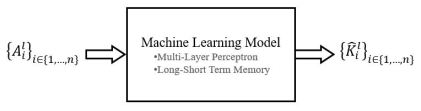
Figure 2: High-level architecture that shows the inputs and outputs at each slot $l$ for the ML techniques that are used in the comparison with the ARNN, where $\hat{K}_{i}^{l}$ denotes the predicted compromised ratio of IP Address $i$ at slot $l$ by any considered ML model.

Then, based on these input-output sets, each ML model is used as follows:

• MLP, which is a feedforward (fully-connected) neural network, is comprised of three hidden layers and an output layer, where there are $n$ neurons at each layer. A sigmoidal activation function is used for each neuron in the network.

• LSTM, which is a recurrent neural network, is comprised of an lstm layer, two hidden layers and an output layer, where there are $n$ lstm units or neurons at each layer. A sigmoidal activation function is used for each neuron in the network.

5 Experimental Results

We now evaluate the performance of the ARNN model and compare it with the performance of some existing techniques for Experiment I and Experiment II, respectively. Note that we set the learning rate $\eta=0.1$ in the algorithm of A.

5.1 Experiment I - Offline Training of the ARNN

We set $\Theta=0.3$ and $0.96\leq\gamma\leq 1$, and summarize the statistics of Accuracy, True Negative Rate (TNR) and True Positive Rate (TNR) performances of ARNN, which are presented in detail in Figures 4, 5, and 6, respectively. Figure 3 displays a box-plot that shows the statistics over all the IP Addresses. These results show that ARNN achieves a high performance with very few outliers in regards of Accuracy, TNR, and TPR. The median accuracy is about $92\%$ while the first quartile is at $87\%$; that is, accuracy is above $87\%$ for $75\%$ of IP addresses. The median of TNR is almost $100\%$; that is, there are almost no false alarms (TNR$=100\%$) for more than $50\%$ of IP addresses. Also, the median of TPR equals $100\%$ and the first quartile is about $62\%$. Thus the TPR equals $100\%$ for more than $50\%$ of IP addresses while it is lower than $62\%$ for only less than $25\%$ of addresses.

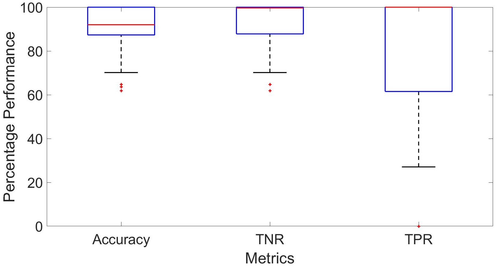
Figure 3: Box-plots of the Accuracy, TNR and TPR performance of ARNN over IP Addresses, where each of box-plot shows the calculated statistics (e.g. median) based on the results presented in Figures 4, 5, and 6, respectively

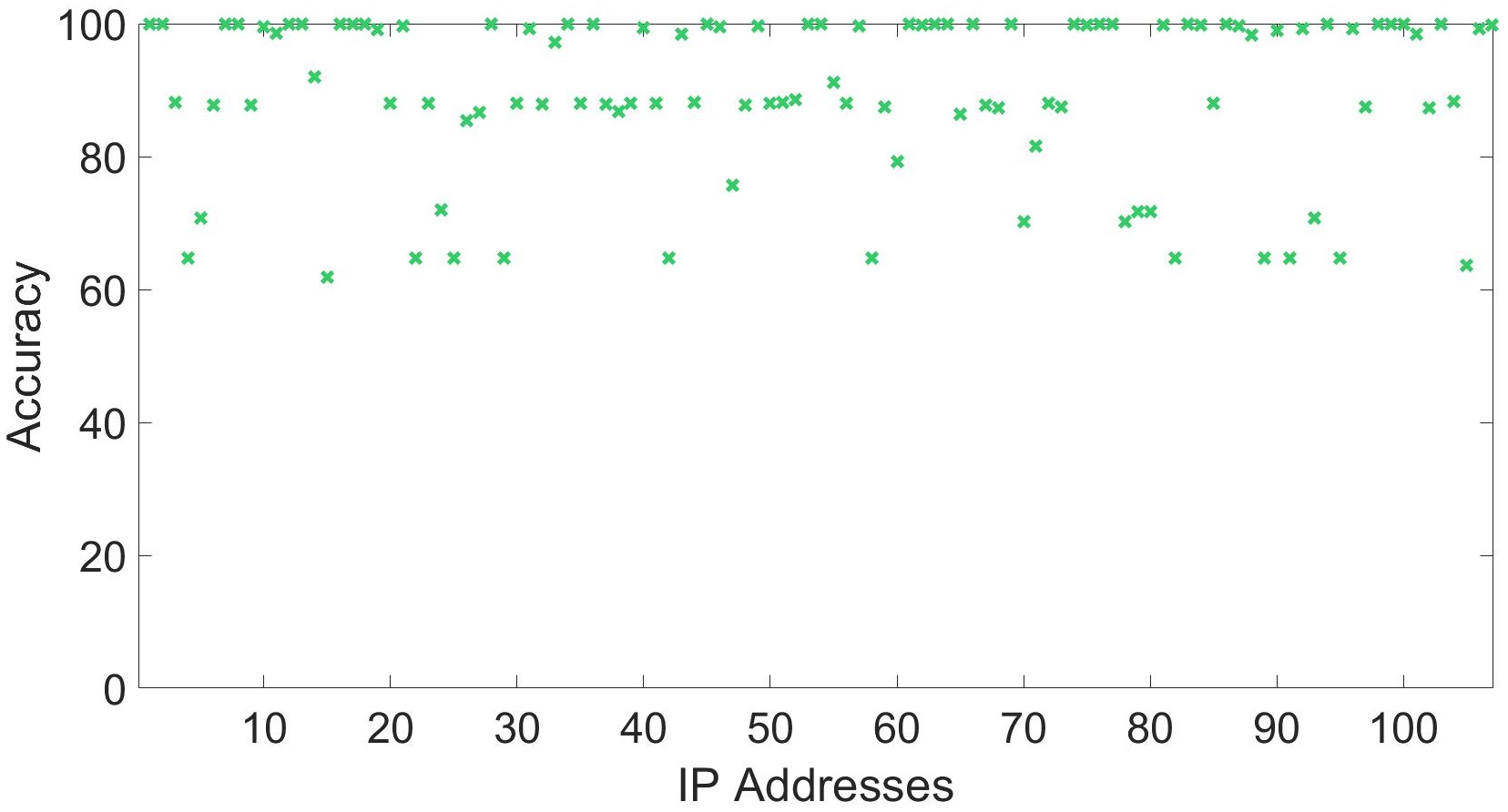
Figure 4: Evaluation of the average accuracy over all packets of each IP Address $i\in\{1,\dots,107\}$ in ${\bf TestData}$. The accuracy is computed by comparing the binary decision in the ground truth $G_{i}^{l}$ and the binary decision of ARNN $Z_{i}^{l}$.

Figure 5: Evaluation of the average percentage TNR over all packets of each IP Address $i\in\{1,\dots,107\}$ in ${\bf TestData}$. For each $i$, TNR is computed by comparing $G_{i}^{l}$ and $Z_{i}^{l}$ for the values of $l$ where $G_{i}^{l}=0$.

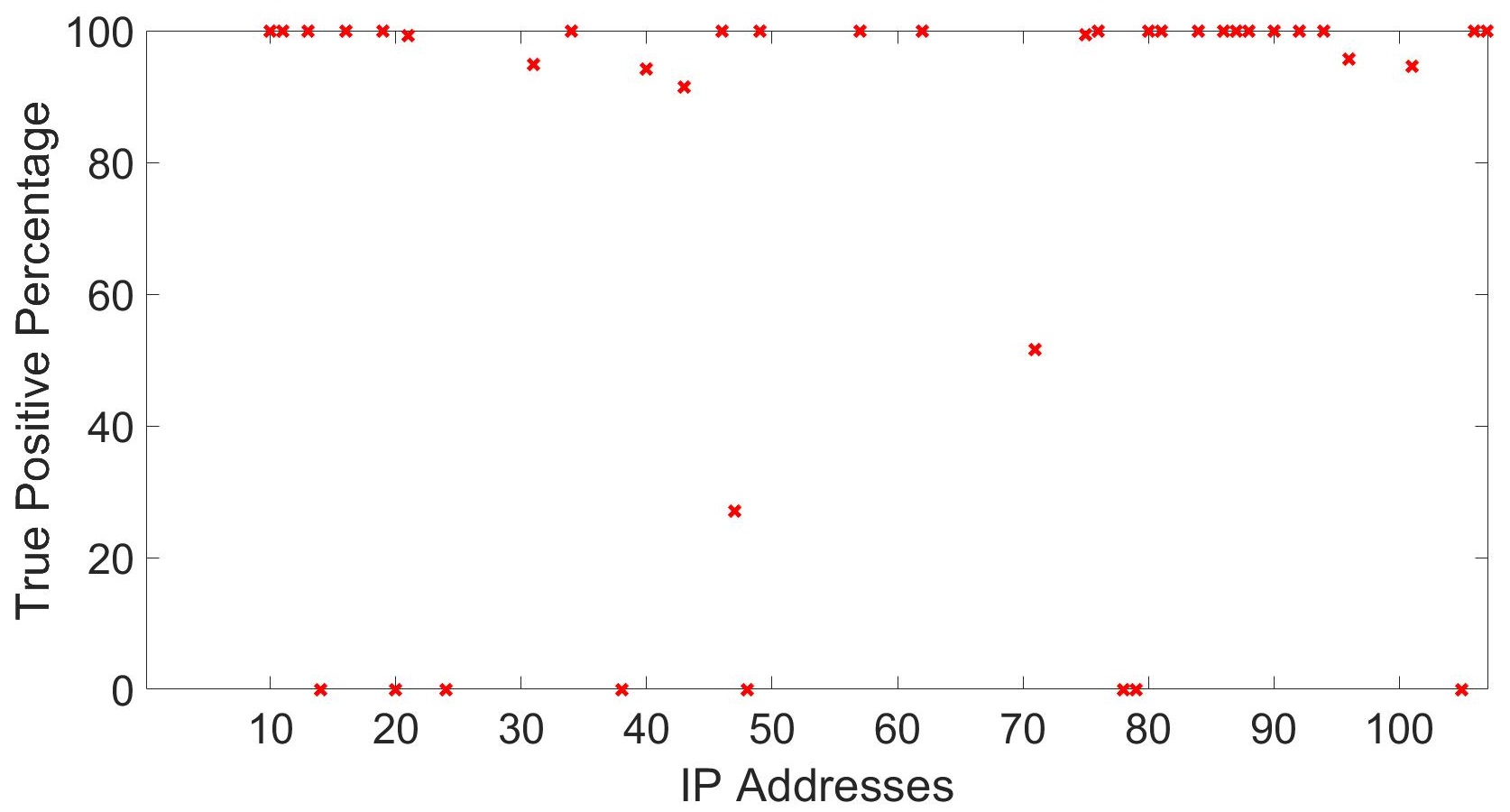
Figure 6: Evaluation of the average percentage TPR over all packets of each IP Address $i\in\{1,\dots,107\}$ in ${\bf TestData}$. For each $i$, TPR is computed by comparing $G_{i}^{l}$ and $Z_{i}^{l}$ for the values of $l$ where $G_{i}^{l}=1$. Note that if $G_{i}^{l}=0$ for an IP Address $i$ for any $l$ in ${\bf TestData}$ (that is, the ground truth indicates that IP Address $i$ has not been compromised within the observation period of the dataset), TPR does not exist for $i$. Accordingly, in the considered dataset TPR exists for $39$ IP Address.

Figure 4 displays the average decision accuracy for each IP Address $i\in\{1,\dots,107\}$. The results in this figure show that the accuracy of ARNN is above $95\%$ for $50\%$ of the IP Addresses while it is between $62\%$ and $80\%$ for only $20\%$ of addresses and does not decrease below $62\%$. Next, Figure 5 presents average percentage TNR of ARNN for each IP Address. The results in this figure show that TNR is above $95\%$ for $59\%$ of all IP Addresses, and it is between $62\%$ and $80\%$ for $15\%$ of addresses. Lastly, Figure 6 displays the percentage average TPR for $39$ IP Addresses for which are considered compromised at least once in the ground truth. The results in this figure show that TPR is greater than $95\%$ for $64\%$ of IP addresses while it is above $90\%$ for more than $74\%$ of the addresses.

5.2 Online (Incremental) Training of the ARNN

Having set $\Theta=0.3$ and $0.96\leq\gamma\leq 1$, we obtain the Accuracy, TNR, and TPR of ARNN with online training shown in Figure 10 in the form of box-plots. In this figure, we see that median accuracy equals $92\%$ while the first quartile equals $87\%$. That is, the accuracy is above $87\%$ for $75\%$ of all IP Addresses. The TNR is above $99\%$ for at least $50\%$ of IP Addresses. The median TPR equals $100\%$; that is, at least $50\%$ (exactly $62\%$) of IP Addresses are $100\%$ accurately identified as compromised. When the results in Experiment II in Figure 7 are compared with those of Experiment I of Figure 3, we see that TPR increases slightly with online training and TNR remains almost the same. In addition, recall that online training is simpler since it does not require data collection, as offline training does.

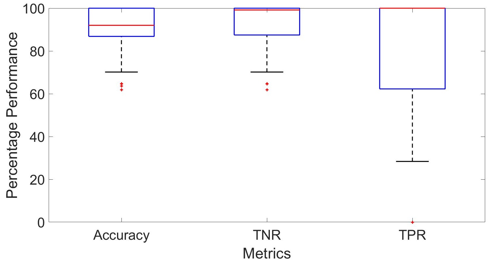
Figure 7: Box-plots of the Accuracy, TNR and TPR performance of ARNN over all IP Addresses, where each box-plot shows the calculated statistics (e.g. median) based on the results presented in Figures 8, 9, and 10, respectively

Figure 8 presents the average accuracy of ARNN for each IP Address $i$ is displayed. The results in this figure show that the accuracy of ARNN is above $95\%$ for $50\%$ of IP Addresses while it is between $62\%$ and $80\%$ for only $20\%$ of addresses and does not decrease below $62\%$. Next, we present the average percentage TNR in Figure 9, and show that the TNR is above $95\%$ for $59\%$ of IP Addresses. Moreover, Figure 10 displays the average percentage TPR for individual IP Addresses, where for IP Address $i$, TPR is presented only if $G_{i}^{l}=1$ for at least a single value of $l$. The results in this figure show that percentage TPR is greater than $95\%$ for $72\%$ of IP Addresses, while TPR under offline training is shown (in Fig. 6) to be above $95\%$ for $64\%$ of IP Addresses. Hence, one may observe that ARNN achieves significantly higher TPR when it is trained online.

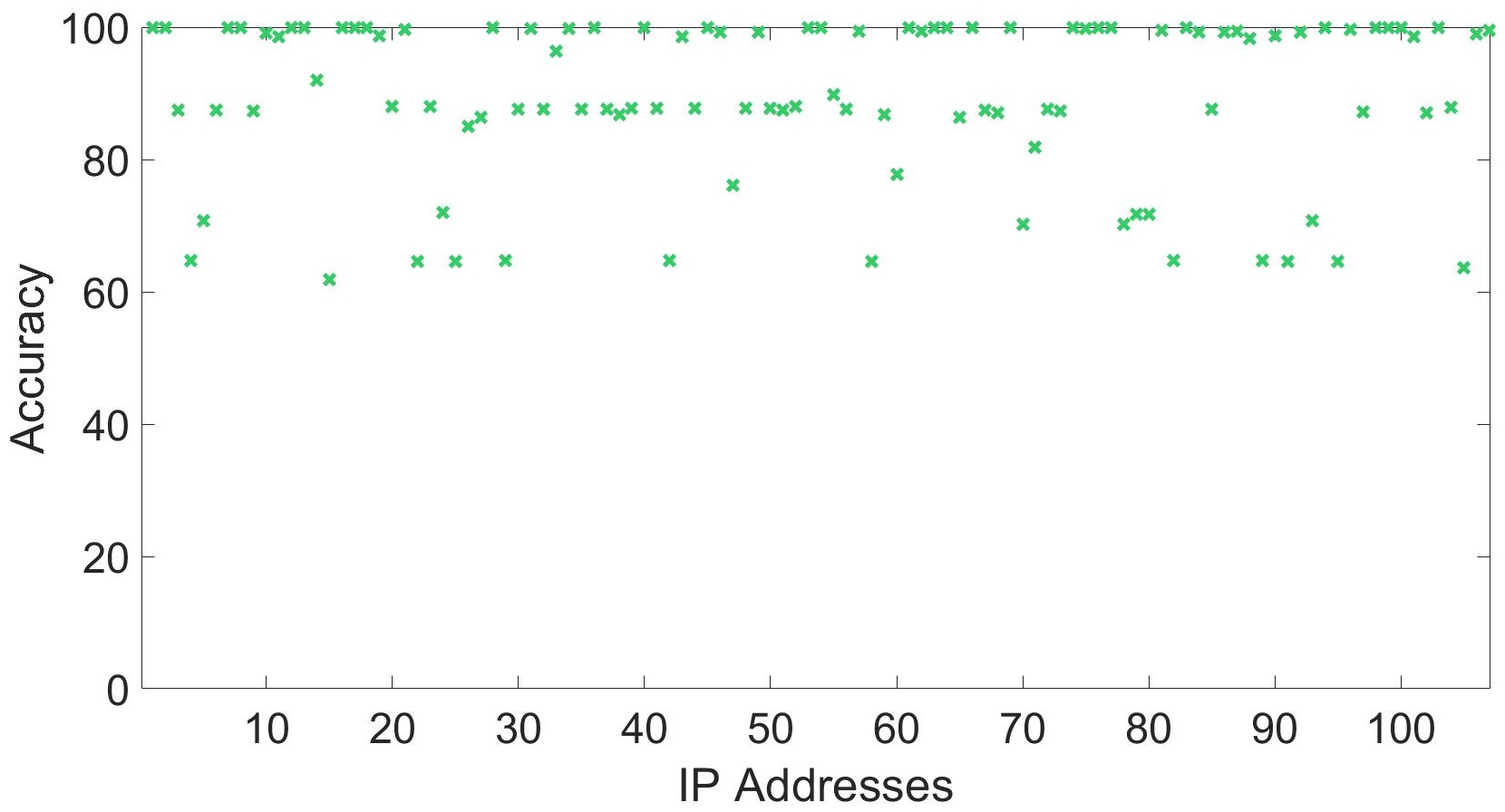
Figure 8: Evaluation of the average accuracy over all packets of each IP Address $i\in\{1,\dots,107\}$. The accuracy is computed by comparing the binary decision in the ground truth $G_{i}^{l}$ and the binary decision of ARNN $Z_{i}^{l}$.

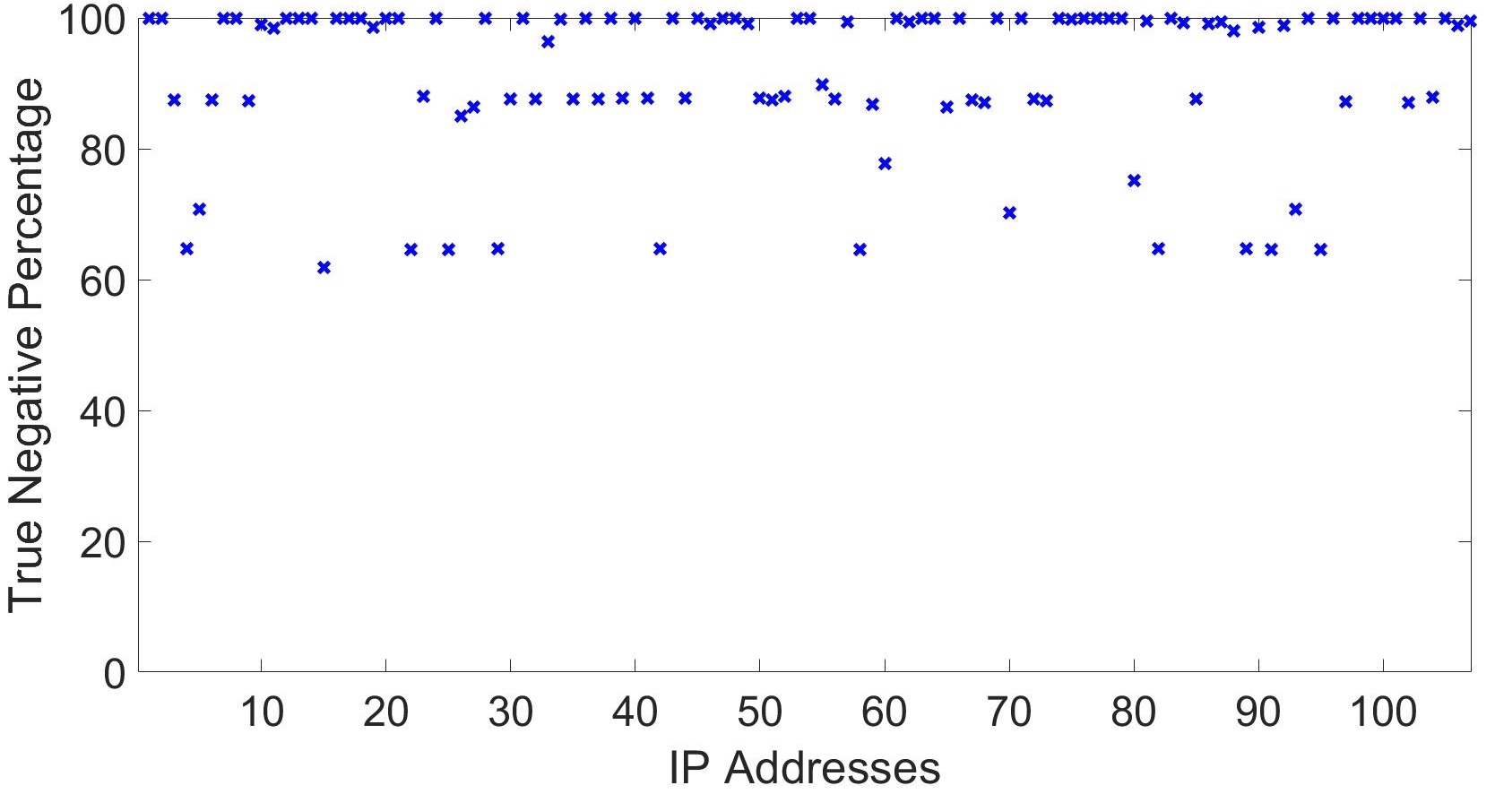
Figure 9: Evaluation of the average percentage TNR over all packets of each IP Address $i\in\{1,\dots,107\}$. For each $i$, TNR is computed by comparing $G_{i}^{l}$ and $Z_{i}^{l}$ for the values of $l$ where $G_{i}^{l}=0$.

Figure 10: Evaluation of the average percentage TPR over all packets of each IP Address $i\in\{1,\dots,107\}$ in ${\bf TestData}$. For each $i$, TPR is computed by comparing $G_{i}^{l}$ and $Z_{i}^{l}$ for the values of $l$ where $G_{i}^{l}=1$. Note that if $G_{i}^{l}=0$ for an IP Address $i$ for any $l$ (that is, the ground truth indicates that IP Address $i$ has not been compromised within the observation period of the dataset), TPR does not exist for $i$. Accordingly, in the considered dataset TPR exists for $39$ IP Address.

5.3 Performance Comparison

We now compare the performance of ARNN with that of MLP and LSTM neural networks with respect to the mean of each Accuracy, TNR, TPR, and F1 Score. The traditional F-measure or $F_{1}$ score is computed as

$$F_{1}=2\frac{Precision.Recall}{Precision+Recall}=\frac{TP}{TP+\frac{1}{2}(FP+FN)},$$ (16)

First, Figure 11 presents the performance comparison of neural network models for Experiment I (offline training), where the results show that the ARNN model significantly outperforms all of the other techniques with respect to all Accuracy, F1 Score, TNR, and TPR. In addition, we also see that LSTM is more successful than MLP for identifying uncompromised nodes (Figure 11 (bottom left)) while MLP identifies the compromised nodes more successfully than LSTM (Figure 11 (bottom right)). However, ARNN outperforms LSTM by $24\%$ with respect to TNR and MLP by $13\%$ with respect to TPR.

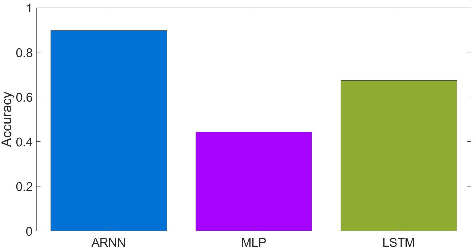
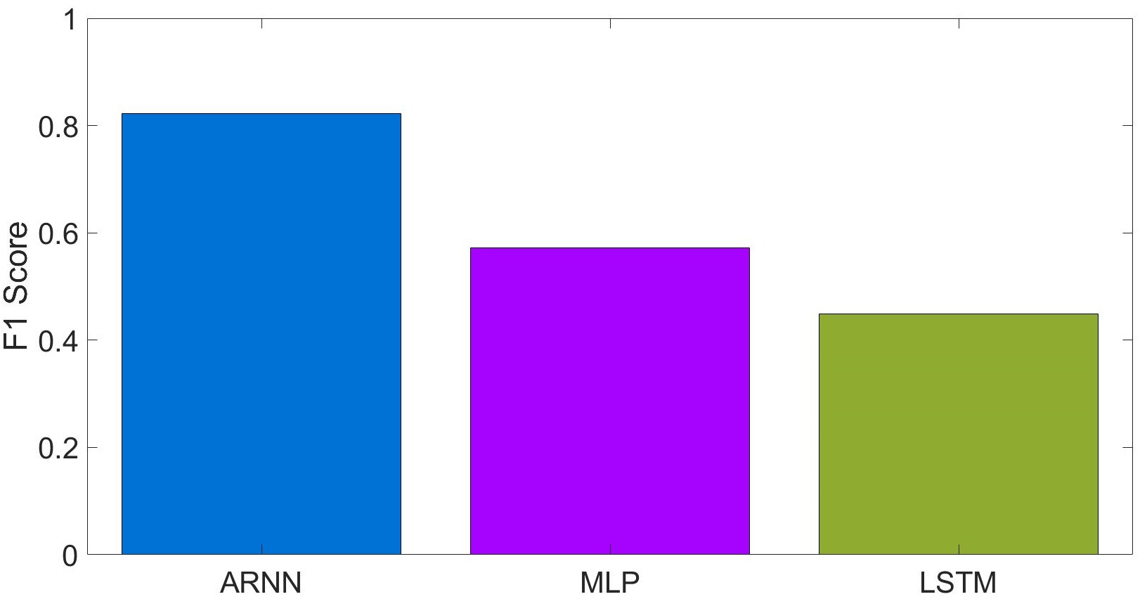
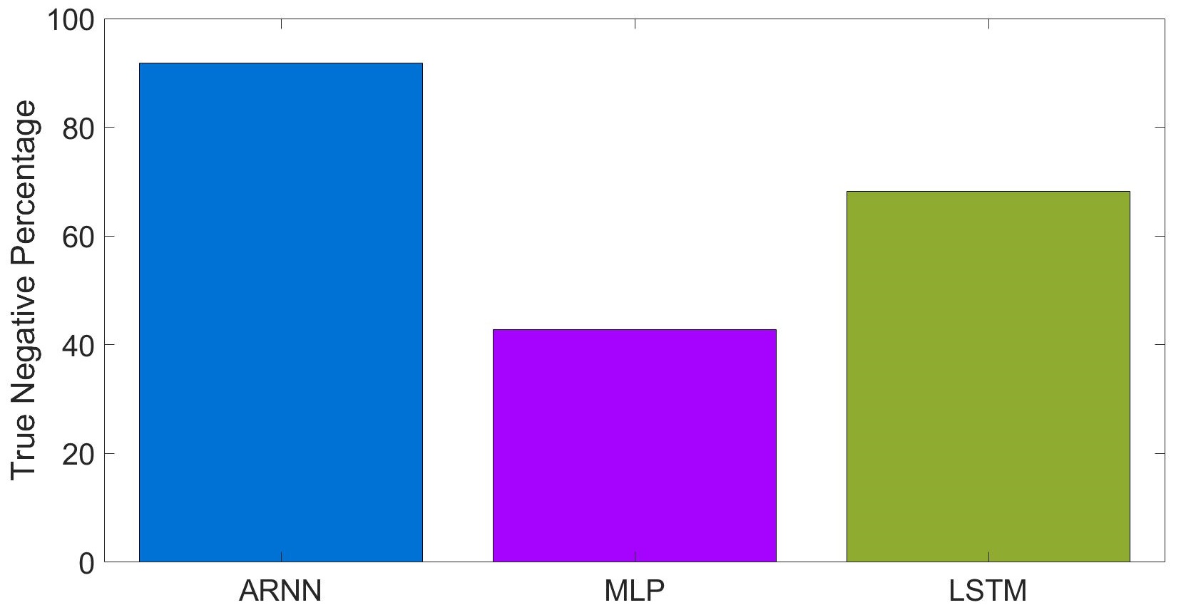
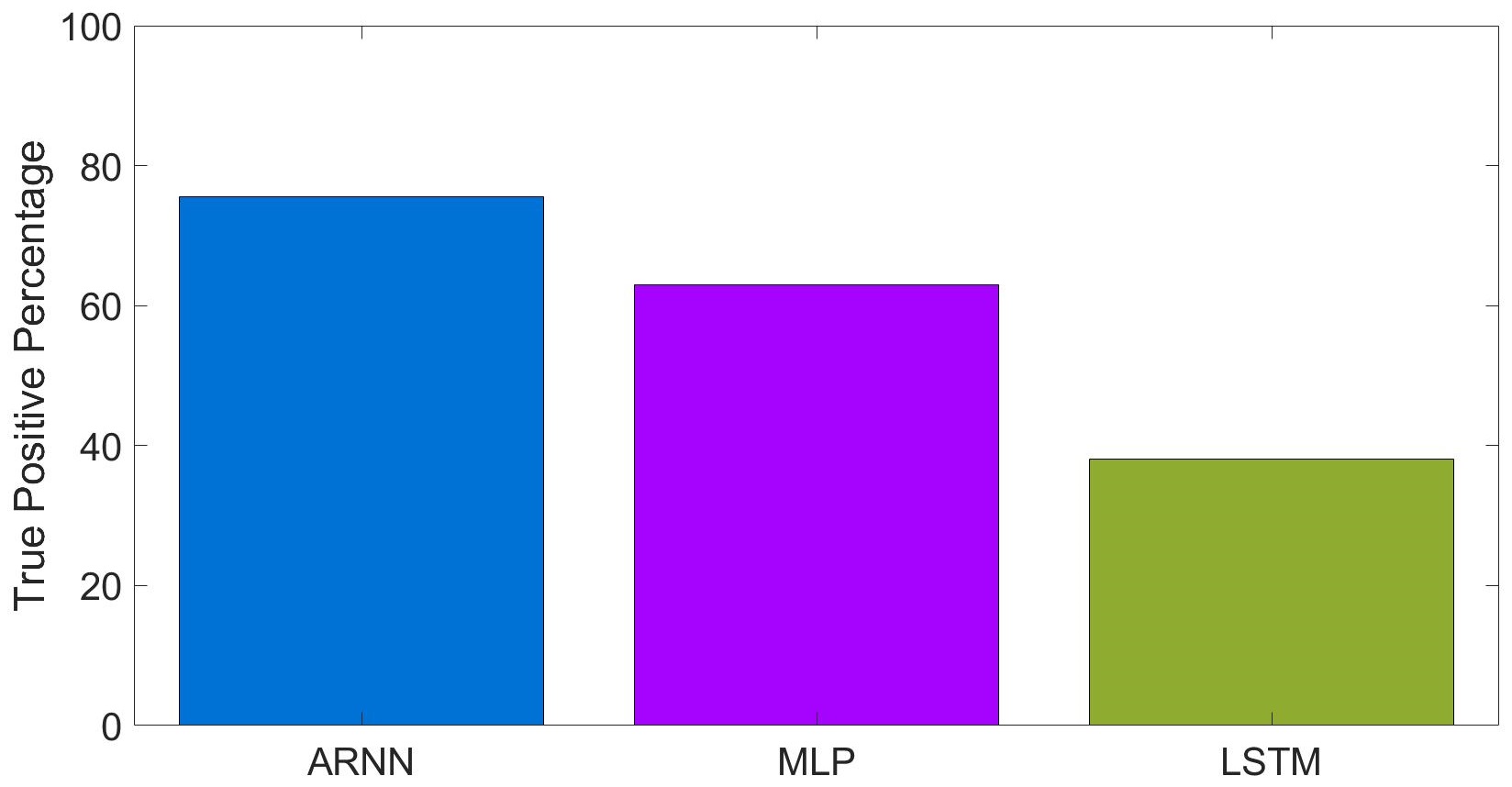
Figure 11: Performance comparison between ARNN, MLP and LSTM for Experiment I (where each model is trained offline) with respect to (top left) Accuracy, (top right) F1 Score, (bottom left) percentage TNR, and (bottom right) percentage TPR

Then, in Figure 12, the comparison of the neural network models for Experiment II (online training) with respect to the mean of each Accuracy, F1 Score, TNR and TPR is presented. The results in this figure show that ARNN significantly outperforms both MLP and LSTM with respect to any measure by at least $27\%$. Moreover, we see that although the overall performances of both MLP and LSTM have been significantly decreased under online training compared with offline training, the performance of ARNN is almost the same under both online and offline training.

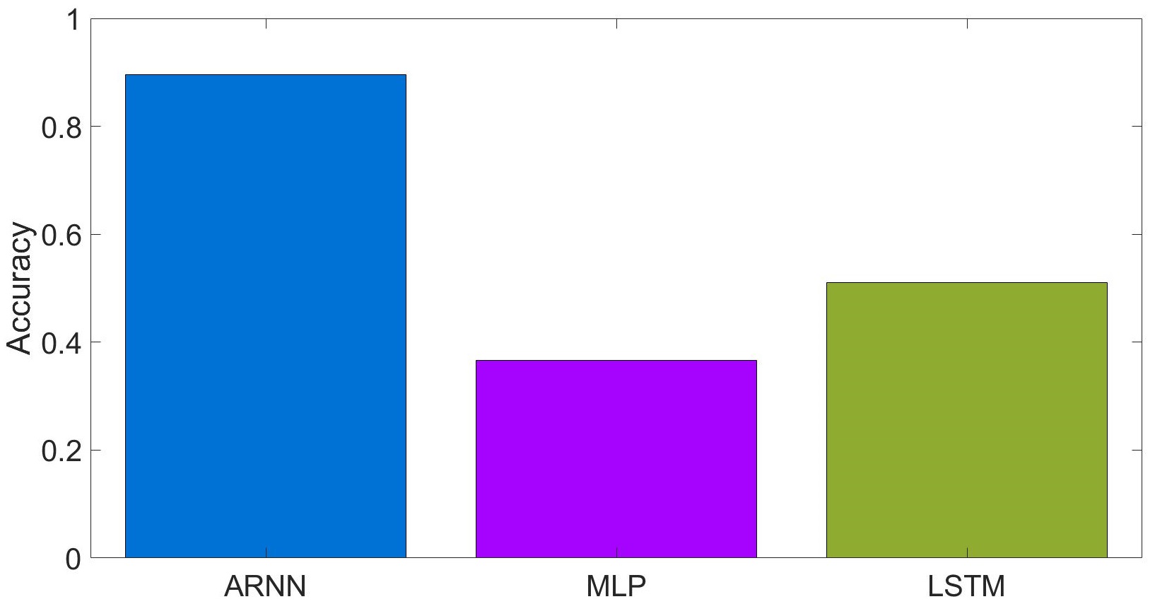
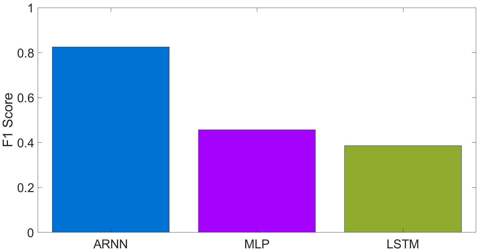
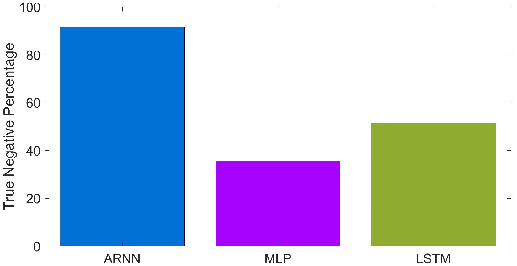
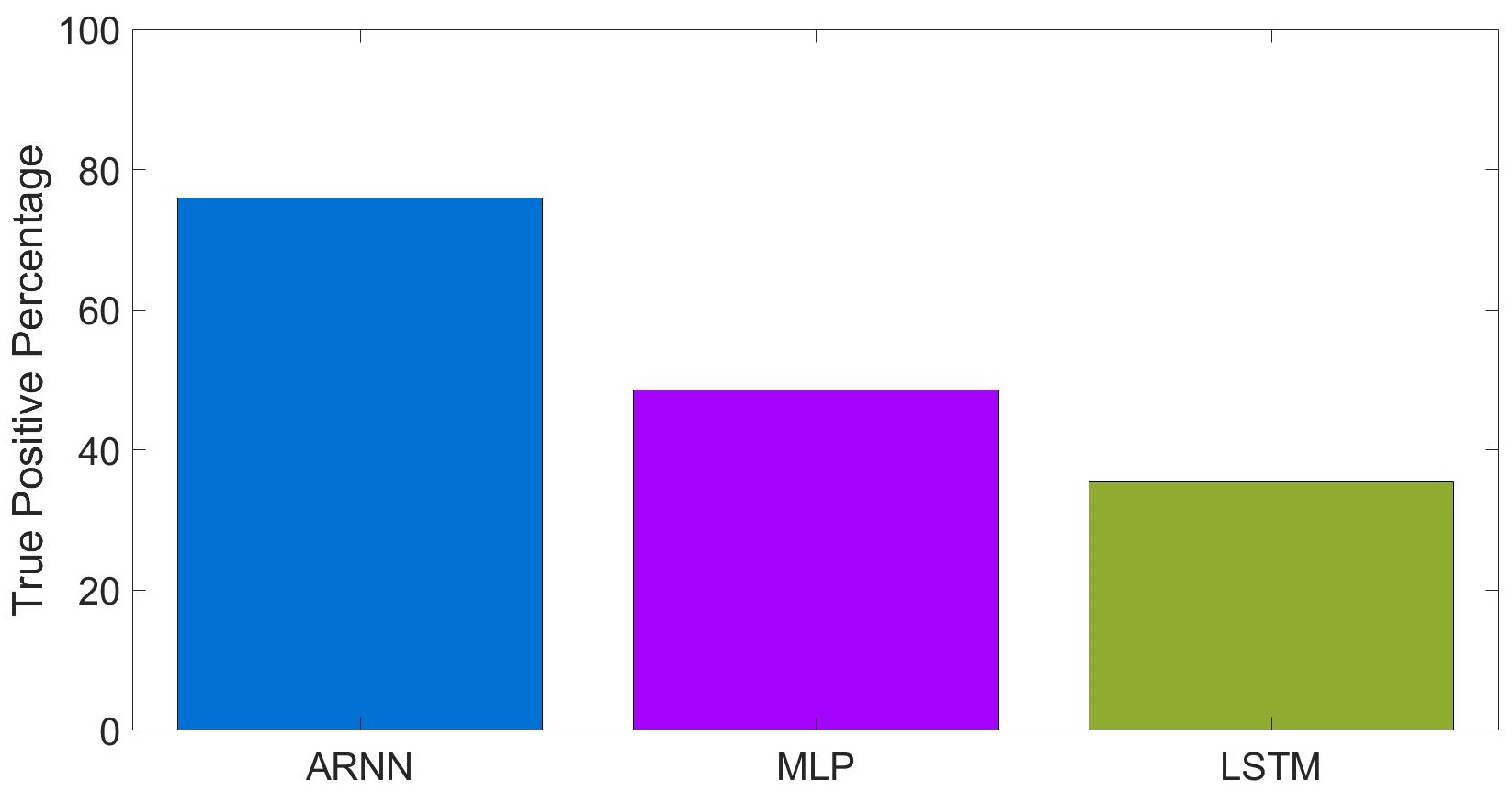
Figure 12: Performance comparison between ARNN, MLP and LSTM for Experiment II (where each model is trained online) with respect to (top left) Accuracy, (top right) F1 Score, (bottom left) percentage TNR, and (bottom right) percentage TPR

5.4 Training and Execution Times

Finally, in Table 1, we present the average training and execution time. Note that these results are collected on a workstation with $32$ Gb RAM and an AMD $3.7$ GHz (Ryzen 7 3700X) processor. The second row of this table displays the average training time that has been spent for a single data sample in a single training step. Thus, during the discussion of the results on training time, we shall calculate the total training time during Experiment I and that for one training window during Experiment II. One should note that both the number of inputs and the number of outputs of ARNN are twice those of MLP and LSTM. One should also note that the implementation of ARNN can be optimized to achieve lower training and execution time, and both MLP and LSTM have been implemented by using Keras library in Python.

Table 1: Average Training Time per Sample per Step and Average Execution Time per Sample of ARNN, MLP and LSTM

	ARNN	MLP	LSTM
Training ($s$)	$40.02$	$3.82\times 10^{-4}$	$0.01$
Execution ($ms$)	$8.4$	$0.17$	$0.78$

During Experiment I, ARNN, MLP and LSTM have been trained on 25 samples for 20 epochs, 1000 epochs and 1000 epochs, respectively. Accordingly, the total training time of these models are $40.02\times 25\times 20=20010~{}s$, $3.82\times 10^{-4}\times 25\times 1000=9.55~{}s$, and $0.01\times 25\times 1000=250~{}s$, respectively. We see that the training time of ARNN is much higher than those of the other models. However, ARNN can be selected as identification method while the training of all models in Experiment I is performed offline and ARNN achieves significantly higher accuracy than MLP and LSTM.

During Experiment II, all three models have been trained online on 1 minute windows (6 samples) for 3 epochs, 100 epochs and 100 epochs respectively. Accordingly, the total training time of these models for each window are $40.02\times 6\times 3=720.36~{}s$, $3.82\times 10^{-4}\times 6\times 100=0.23~{}s$, and $0.01\times 6\times 100=6~{}s$, respectively. Although the training time results show that MLP and LSTM are suitable for training once in 1 minute, the performance of either MLP or LSTM has shown not to be acceptable for practical usage. On the other hand, ARNN with its current implementation achieves high accuracy but can be trained once in 720.36 seconds ($\approx$12 minutes) on 1 minute of data.

Furthermore, the third row of this table displays the average execution time that has been spent to make a prediction for a single sample. The results in this row show that the execution time of ARNN is one order of magnitude higher than the execution times of MLP and LSTM.

6 Conclusions

In a network of IP addresses, when n individual node is attacked by a Botnet and becomes compromised, it can then compromise other network nodes and turn them into attackers. Thus attacks may propagate across the system and affect other nodes and IP addresses. There is a large prior literature regarding Botnet attacks, but most of the work has addressed attacks against a specific network node, while the collective detection of Botnet attacks has received less attention.

Thus in this paper we have developed a ML based decision method, that identifies all the nodes of a given interconnected set of nodes, that are compromised by a Botnet attack. The approach is based on designing an Associated Random Neural Network that incorporates two connected and recurrent Random Neural Networks (RNN), where each RNN offers a contradictory recommendation regarding whether any one of the IP addresses or network nodes in the system are compromised. The final decision is taken by the ARNN based on which of the two recommendations for each of the nodes appears to be stronger. We have also developed a gradient based learning algorithm for the ARNN, which learns based on linear-algebraic operations on the network weights. If the system is composed of $n$ IP addresses or nodes, then the resulting learning algorithm is of time complexity $O(n^{3})$ since all computations are based on the inversion of $n\times n$ matrices.

In this paper, the ARNN and its learning algorithm have been described and tested on real Botnet data involving some $760,000$ packets. The experimental results show that the ARNN provides very accurate predictions of the order of $92\%$ for a $107$ node network. For comparison purposes, we have also implemented and tested two well known ML approaches for the same training and testing datasets, showing that the ARNN results provide significantly much better accuracy.

In future work, we plan to develop a generalization of the ARNN for multiple valued binary collective decision making and classification in other significant areas with datasets that contain inter-related or inter-dependent data items, such as social networks and the analysis of epidemics.

Appendix A Appendix: ARNN Learning Algorithm

In this Appendix, we focus on the ARNN’s learning algorithm, recalling that the ARNN is a specific ML structure based on the Random Neural Network (RNN), which has been proven to be an effective approximator in the sense of [80] for continuous and bounded functions [81]. It was generalized to G-Networks in the framework of queueing theory [82, 83, 84]. Gradient learning for the RNN was initially designed for both feedforward and recurrent (feedback) RNNs [77], and other RNN learning algorithms have also been proposed [37, 85, 72].

Prior to running the learning algorithm, the ARNN parameters are set to “neutral” values which express the fact that initially the ARNN does not know whether any of the network nodes are compromised. To this effect, we:

• Initialize all the weights between $X_{i}$ and $Y_{i}$ to zero: $W^{+}_{ii}=w^{+}_{ii}=W^{-}_{ii}=w^{-}_{ii}=0$.

• Set $W^{+}_{ij}=W^{-}_{ij}=w^{+}_{ij}=w^{-}_{ij}=0.5W$ for $i\neq j$, and choose $Q_{i}=q_{i}=0.5$ to represent the perfect ignorance of the ARNN.

• Set the external inputs of the ARNN to $\Lambda_{i}=\lambda_{i}=L(n-1),~{}L>0$, so that the external excitatory and inhibitory inputs are all initially set to an identical value.

• Keep $W$ constant in the learning procedure, and only learn $W^{+}_{ij},~{}w^{+}_{ij}$ for each $i\neq j$.

• Accordingly (8) becomes:

  $$q_{i}=Q_{i}=0.5$$ (17)

  $$=\frac{L(n-1)+0.25(n-1)W}{L(n-1)+(n-1)W+0.25(n-1)W},$$

  $$or~{}0.5=\frac{L+0.25W}{L+W+0.25W},$$

  $$yielding~{}L=0.75W~{}.$$ (18)

• Taking $W=1$ and $L=0.75$, all the neuron states are initialized with the values $Q_{i}=q_{i}=0.5,~{}i=1,~{}...~{},n$.

Now for any given value of the data, we use gradient descent to update the ARNN weights so as to search for a local minimum of the error ${\bf E}$ in equation (14). We drop the notation regarding the $l-th$ data item for simplicity, and compute ${\bf E}$’s derivative with respect to each of the ARNN weights:

$$E^{U,V}\equiv\frac{\partial{\bf E}}{\partial W^{+}_{U,V}}$$

$$=\sum_{i=1}^{n}~{}[~{}(Q_{i}-K_{i})Q^{U,V}_{i}+(q_{i}-1+K_{i})q^{U,V}_{i}~{}],$$ (19)

$$E^{u,v}\equiv\frac{\partial{\bf E}}{\partial w^{+}_{u,v}}$$

$$=\sum_{i=1}^{n}~{}[~{}(Q_{i}-K_{i})Q^{u,v}_{i}+(q_{i}-1+K_{i})q^{u,v}_{i}~{}],$$ (20)

where the derivatives of the ARNN state values are denoted:

$$Q^{U,V}_{i}=\frac{\partial Q_{i}}{\partial W^{+}_{U,V}},~{}Q^{u,v}_{i}=\frac{\partial Q_{i}}{\partial w^{+}_{u,v}},$$

$$q^{U,V}_{i}=\frac{\partial q_{i}}{\partial W^{+}_{U,V}},~{}q^{u,v}_{i}=\frac{\partial q_{i}}{\partial w^{+}_{u,v}}.$$

We can then use the expressions (19) and (20) to update the ARNN weights iteratively for successive values of $d=1,~{}...~{},|\textbf{TrainData}|$, with the Gradient Descent Rule with some $\eta>0$:

$$W^{+}_{new,U,V}\leftarrow W^{+}_{U,V}-\eta E^{U,V}|_{(V^{d},v^{d})},$$

$$w^{+}_{new,U,V}\leftarrow w^{+}_{u,v}-\eta E^{u,v}|_{(V^{d},v^{d})}.$$ (21)

A.1 Derivatives of the ARNN State Probabilities

Now consider the ARNN with generic inputs $\Lambda=(\Lambda_{1},~{}...~{}\Lambda_{n})$ and $\lambda=(\lambda_{1},~{}...~{},\lambda_{n})$. In order to obtain the derivatives needed for the gradient descent expression (21), we use (8) to write:

$$Q^{U,V}_{i}=\frac{Q_{U}}{D_{V}}1[i=V]+\sum_{j=1}^{n}\frac{W^{+}_{ji}}{D_{i}}~{}Q^{U,V}_{j}$$

$$~{}~{}~{}~{}~{}~{}~{}-\sum_{j=1}^{n}\frac{Q_{i}[W-w^{+}_{ji}]}{D_{i}}~{}q^{U,V}_{j},$$ (22)

$$q^{U,V}_{i}=\sum_{j=1}^{n}\frac{w^{+}_{ji}}{d_{i}}~{}q^{U,V}_{j}-\sum_{j=1}^{n}\frac{q_{i}[W-W^{+}_{ji}]}{d_{i}}~{}Q^{U,V}_{j}$$

$$~{}~{}~{}~{}~{}~{}~{}+\frac{q_{U}}{d_{V}}1[i=V],$$ (23)

where $D_{i}$ and $d_{i}$ are the denominators of $Q_{i}$ and $q_{i}$ respectively, in (8):

$$D_{i}=\Lambda_{i}+\sum_{j=1,j\neq i}^{n}W+\sum_{j=1,j\neq i}^{n}[W-w^{+}_{ji}]~{}.q_{j},$$ (24)

$$d_{i}=\lambda_{i}+\sum_{j=1,j\neq i}^{n}W+\sum_{j=1,j\neq i}^{n}[W-W^{+}_{ji}]~{}.Q_{j}.$$

Define the vectors $Q=(Q_{1},~{}...~{},Q_{n})$ and $q=(q_{1},~{}...~{},q_{n})$ and the corresponding vectors of derivatives $Q^{U,V}=(Q^{U,V}_{1},~{}...~{},Q^{U,V}_{n})$ and $q^{U,V}=(q^{U,V}_{1},~{}...~{},q^{U,V}_{n})$. Similarly we define the $n\times n$ matrices:

$$B^{+}=\{\frac{W^{+}_{ij}}{D_{j}}\},~{}C=\{\frac{Q_{j}[W-w^{+}_{ij}]}{D_{j}}\},$$ (25)

$$F^{+}=\{\frac{w^{+}_{ij}}{d_{j}}\},~{}G=\{\frac{q_{j}[W-W^{+}_{ij}]}{d_{j}}\}.$$

We use the vector $\delta_{V}$ whose elements are zero everywhere, except in position $V$ where the value is $1$, and write (22) and (23) in vector form:

$$Q^{U,V} = B^{+}Q^{U,V}-Cq^{U,V}+\delta_{V}.\frac{Q_{U}}{D_{V}},$$

$$q^{U,V} = F^{+}q^{U,V}-GQ^{U,V}+\frac{q_{U}}{d_{V}}\delta_{V},$$ (26)

$$= [-GQ^{U,V}+\frac{q_{U}}{d_{V}}\delta_{V}][I-F^{+}]^{-1},$$

which yields:

$$Q^{U,V}=B^{+}Q^{U,V}+[CGQ^{U,V}-\frac{q_{U}}{d_{V}}C\delta_{V}][1-F^{+}]^{-1}+\delta_{V}.\frac{Q_{U}}{D_{V}},$$

and hence:

$$Q^{U,V}=\{-\frac{q_{U}}{d_{V}}C\delta_{V}[I-F^{+}]^{-1}+\frac{Q_{U}}{D_{V}}\delta_{V}\}{\bf.}$$ (27)

$$~{}~{}~{}~{}~{}~{}~{}~{}{\bf.}\{I-B^{+}-CG[I-F^{+}]^{-1}\}^{-1}\qquad$$

Also define the matrices:

$$B_{*}^{+}=\{\frac{w^{+}_{ij}}{d_{j}}\},~{}C_{*}=\{\frac{q_{j}[W-W^{+}_{ij}]}{d_{j}}\},$$ (28)

$$F_{*}^{+}=\{\frac{W^{+}_{ij}}{D_{j}}\},~{}G_{*}=\{\frac{Q_{j}[W-w^{+}_{ij}]}{D_{j}}\}.$$

Since $Q^{U,V}$ and $q^{u,v}$ are symmetric with respect to each other, as are $Q^{u,v}$ and $q^{U,V}$, we also obtain:

$$q^{u,v}=\{-\frac{Q_{u}}{D_{v}}C_{*}\delta_{v}[I-F_{*}^{+}]^{-1}+\frac{q_{u}}{d_{v}}\delta_{v}\}{\bf.}$$

$$~{}~{}~{}~{}~{}~{}{\bf.}\{I-B_{*}^{+}-C_{*}G_{*}[I-F_{*}^{+}]^{-1}\}^{-1},$$ (29)

and

$$Q^{u,v}=\{-G_{*}q^{u,v}+\frac{Q_{u}}{D_{v}}\delta_{v}\}[I-F_{*}^{+}]^{-1}~{}.$$ (30)

This completes the computation of all the needed derivatives of the ARNN state probability vectors $Q$ and $q$.

References

- [1] W. R. Schwartz, H. Guo, J. Choi, L. S. Davis, Face identification using large feature sets, IEEE Transactions on Image Processing 21 (4) (2012) 2245–2255. doi:10.1109/TIP.2011.2176951.
-
[2]
A. Ortner,
Top
10 binary classification algorithms [a beginner’s guide] (May 2020).
URL https://github.com/alexortner/teaching/tree/master/binary_classification -
[3]
T. A. Tuan, H. V. Long, L. H. Son, R. Kumar, I. Priyadarshini, N. T. K. Son,
Performance evaluation of
botnet ddos attack detection using machine learning, Evolutionary
Intelligence (October 2019).
URL https://doi.org/10.1007/s12065-019-00310-w - [4] K. Filus, J. Domańska, E. Gelenbe, Random neural network for lightweight attack detection in the IoT, in: Symposium on Modelling, Analysis, and Simulation of Computer and Telecommunication Systems, Springer, Cham, 2021, pp. 79–91.
- [5] M. Alshamkhany, W. Alshamkhany, M. Mansour, M. Khan, S. Dhou, F. Aloul, Botnet attack detection using machine learning, in: 14th International Conference on Innovations in Information Technology (IIT), 2020, pp. 203–208. doi:10.1109/IIT50501.2020.9299061.
- [6] E. Gelenbe, M. Nakıp, Traffic based sequential learning during Botnet attacks to identify compromised iot devices, IEEE Access 10 (2022) 126536–126549. doi:10.1109/ACCESS.2022.3226700.
- [7] M. Bilgic, G. M. Namata, L. Getoor, Combining collective classification and link prediction, in: Seventh IEEE International Conference on Data Mining Workshops (ICDMW 2007), 2007, pp. 381–386. doi:10.1109/ICDMW.2007.35.
-
[8]
P. Sen, G. Namata, M. Bilgic, L. Getoor,