Gamma-rays and neutrinos from supernovae of Type Ib/c with late time emission

Abstract

Observations of some supernovae (SNe), such as SN 2014C, in the X-ray and radio wavebands revealed a rebrightening over a timescale of about a year since their detection. Such a discovery hints towards the evolution of a hydrogen-poor SN of Type Ib/c into a hydrogen-rich SN of Type IIn, the late time activity being attributed to the interaction of the SN ejecta with a dense hydrogen-rich circumstellar medium (CSM) far away from the stellar core. We compute the neutrino and gamma-ray emission from these SNe, considering interactions between the shock accelerated protons and the non-relativistic CSM protons. Assuming three CSM models inspired by recent electromagnetic observations, we explore the dependence of the expected multi-messenger signals on the CSM characteristics. The detection prospects of existing and upcoming gamma-ray (Fermi-LAT and Cerenkov Telescope Array) and neutrino (IceCube and IceCube-Gen2) telescopes are also outlines. Our findings are in agreement with the non-detection of neutrinos and gamma-rays from past SNe exhibiting late time emission. Nevertheless, the detection prospects of SNe with late time emission in gamma-rays and neutrinos with the Cerenkov Telescope Array and IceCube-Gen2 (Fermi-LAT and IceCube) are promising and could potentially provide new insight into the CSM properties, if the SN burst should occur within $10$ Mpc ($4$ Mpc).

I Introduction

Supernovae (SNe) Ib/c are among the dominant SN types ($26\%$) in the local universe [1]. Typically, the light curve of a SN Ib/c fades after a few weeks [2, 3, 4]. However, recent observations of SN 2014C, a SN of Type Ib/c, have revealed that a fraction of SNe of Type Ib/c exhibits evidence of late rebrightening at a few $\mathcal{O}(100)$ days [5, 6, 7]. Such rebrightening resembles the behavior of a hydrogen-rich SN (i.e. a SN of Type IIn). Due to this peculiar feature, SN 2014C has been referred to as “chameleon SN” [6].

The late time (LT) rebrightening may result from the interaction of the SN ejecta with a dense circumstellar medium (CSM) surrounding the dying star. Observations of SN 2014C suggest that the shock may have interacted with a dense hydrogen (H) rich CSM located at larger radii. Such CSM structure could be due to the ejection of the H envelope a few centuries prior to explosion or the interaction of a Wolf-Rayet star wind with a dense red-supergiant wind [8, 6]. In addition, evidence for an asymmetric CSM hints towards an explosion occurring within a binary system [9, 10]. The dense hydrogen rich CSM of SN2014C is found to be located at about $10^{16}$–$10^{17}$ cm, which is at a distance far away from the stellar envelope ($\sim 10^{11}$ cm) and has a mass of about $1$–$2\ \rm M_{\odot}$ [6, 11, 8]. Such dense CSM has also been observed for different types of core collapse SNe [12, 13, 14, 15].

For a wind-like CSM, the CSM density depends on the mass-loss rate ($\dot{M}_{\rm W}$) and the wind velocity ($v_{\rm W}$). The CSM of conventional SNe Ib/c in the first few $100$ days (early phase) exhibits $\dot{M}_{\rm W}\in[10^{-7},10^{-4}]~{}\rm M_{\odot}~{}yr^{-1}$, with $v_{\rm W}$ being approximately $10^{2}$–$10^{3}~{}\rm{km\ s}^{-1}$ [12]. However, $\dot{M}_{\rm W}$ estimated for SN 2014C after about $200$–$300$ days (late phase) is $\mathcal{O}(1)$ $\rm M_{\odot}yr^{-1}$ [6], with $v_{\rm W}\in[10,10^{3}]~{}\rm{km\ s}^{-1}$ that corresponds to a CSM density $\sim 2\times 10^{6}~{}{\rm cm^{-3}}$ at $6\times 10^{16}~{}{\rm cm}$ and then falls as a function of the radius as $r^{-2}$. Analysis of the available X-ray data suggest a constant CSM density up to $8\times 10^{16}~{}{\rm cm}$ which then falls following $r^{-2.5}$ [8]. Recent work focusing on X-ray data from SN 2014C instead infers two different density profiles [16]. One of these density profiles scales as $r^{-1.5\pm 0.01}$, while the other one has a steeper profile falling like $r^{-2.42\pm 0.17}$. Interestingly, this analysis reports that the LT emission from SN 2014C is due to a dense H-rich disk resulting in an asymmetric CSM. These conclusions are in contrast with the model based on a spherically symmetric CSM density profile falling as $r^{-3}$ [11]. Nevertheless, it is clear that the CSM of SN 2014C is different from the ones usually observed with wind-like CSM (i.e., $r^{-2}$ profile).

Similar LT features have been observed for SNe 2003gk, 2004cc, 2004dk, 2004gk, and 2019yvr [6, 16, 17, 18, 19]; additional examples of past SNe Ib/c showing indirect evidence of similar LT activity have been reported in Refs. [6, 16]. All these SNe initially showed properties of usual SNe Ib/c, but later evolved into IIn-like SNe with dense CSM. By relying on current observations, the fraction of SNe Ib/c with LT emission is expected to be about $2.6\%$ of all core-collapse SNe [6, 20]. In the following, we assume SN 2014C as representative of this class of chameleon SNe.

The interaction of the SN ejecta with the CSM may lead to the production of secondary particles, such as neutrinos and gamma-rays, via inelastic proton-proton ($pp$) collisions [21, 22, 23, 24, 4, 25, 26, 27, 28, 29, 30]. The flux of neutrinos and gamma-rays from the conventional early phase of SNe of Type Ib/c was found to be faint, with poor detection prospects (the detection horizon being estimated to be around $2$–$6$ Mpc) [31, 32, 33, 34]. However, due to the presence of the dense hydrogen rich CSM at large radii, the fluxes of neutrinos and gamma-rays from SNe Ib/c LT can be larger than the ones expected in the early SN phase.

Different CSM density profiles may yield different fluxes of neutrinos and gamma-rays. Therefore, the detection of these secondary particles could be crucial to disentangle the properties of the CSM as well as probe the shock acceleration mechanism. In this work, we consider the aforementioned CSM profiles to compute the expected fluxes of neutrinos and gamma-rays and discuss their detection prospects with current and upcoming gamma-ray (Fermi-LAT and CTA) and neutrino (IceCube and IceCube-Gen2) telescopes.

This paper is organized as follows. We introduce the CSM models of the LT emission in Sec. II, followed by the modelling of the neutrino and gamma-ray signals in Sec. III. The temporal evolution, the spectral energy distribution of the secondaries, and their dependence on the model parameters are explored in Sec. IV. The detection prospects of SN 2014C-like bursts with current and future gamma-ray and neutrino telescopes are presented in Sec. V. Finally, we summarize our findings in Sec. VI. The characteristic timescales for proton acceleration and cooling processes are provided in Appendix VI.

II Modeling of the circumstellar medium

Our understanding of the CSM density profile of SN 2014C is still uncertain and different scenarios have been proposed in the literature [6, 8, 11, 16]. In this paper, we consider the following CSM models:

• Model A—A spherically symmetric and dense CSM. The CSM density is assumed to be constant ($n_{\rm CSM}\simeq 10^{6}~{}\rm cm^{-3}$) between the inner radius, $r_{\rm i}$ $\simeq 6\times 10^{16}$ cm and the break radius $r_{\rm b}$ $\simeq 8\times 10^{16}$ cm [8]. The CSM density beyond $r_{\rm b}$ falls as $r^{-2.5}$ up to the outer radius, $r_{\rm o}$ $\simeq 2.5\times 10^{17}$ cm. The origin of the constant CSM is not well understood. It may originate from the interaction of a short lived Wolf-Rayet star wind with the remnant of a dense red supergiant wind [20], due to mass loss [35], or to the ejection of the H envelope caused by binary interactions [8].

• Model B—An asymmetric CSM model [16]. The asymmetry is proposed to be caused by the H-rich disk in the equatorial plane and the observed X-ray emission from SN 2014C is attributed to this disk like CSM [16]. Two different density profiles have been proposed for the disk, one with a density profile falling as $r^{-1.50\pm 0.01}$ and the other with a steeper profile of the form $r^{-2.42\pm 0.17}$. We take into account both density profiles: Model B1 ($r^{-1.5}$) and Model B2 ($r^{-2.42}$).

  To model the asymmetric CSM scenario, we introduce a geometrical (asymmetry) factor, $f$ ($\leq 1$)[16]. The case $f=1$ corresponds to spherical symmetry in the CSM and the most asymmetric (disk-like) CSM is described by $f=0.1$. The degree of the asymmetry of the CSM of SN 2014C is still uncertain. Therefore, to take into account the possibility of different asymmetric scenarios, $f$ is varied between $1.0$ and $0.1$ [16]. The variation of the CSM density is proportional to $f$ for Model B1, whereas it scales as $\sqrt{f}$ for Model B2.

We assume that the CSM ends abruptly at the outer radius ($r_{\rm o}$), for Models A and B. The location of the CSM over density is uncertain [6, 11, 16], hence we choose to keep the location unchanged in both models. Note that these CSM profiles are different with respect to the conventional wind one ($\propto r^{-2}$ [6]), not considered in this paper. Here we refer the reader to Refs. [32, 34] for dedicated work on the production of neutrinos and gamma-rays for the CSM wind profile.

III Spectral energy distributions of gamma-rays and neutrinos

High energy neutrinos and gamma-rays can be produced through the interaction of shock accelerated protons with non-relativistic CSM protons. This proton-proton ($pp$) interaction creates charged and neutral mesons ($\pi$ and $\eta$), which decay into secondaries, such as neutrinos and gamma-rays [21].

The spectral energy distribution of accelerated protons is assumed to be a power-law distribution, $Q_{\rm p}^{\rm inj}(E_{\rm p},r)\propto E_{\rm p}^{-\alpha}\exp\left[{-E_{\rm p}/E_{\rm p,max}(r)}\right]$, where $\alpha$ is the power law index [36, 37, 21, 38, 39, 40, 31]. We consider $\alpha\in[2.0,2.2]$ for our analysis [34, 41, 42, 43]. The choice of $\alpha$ depends on the details of the shock acceleration mechanism, also responsible for efficiently accelerating protons up to PeV energies. In particular, magnetic field amplification can be considered to be the primary requirement for efficient acceleration [44, 45]. For example, plasma instabilities may give rise to small scale magnetic field [46]. Non-resonant hybrid (NRH) instability [47, 48, 49, 50, 51] in YSNe is another possibility. Such instability investigated for SN remnants [47] shows that cosmic rays (CRs) in the upstream shock can excite turbulence amplifying the initial background magnetic field. Such amplification can lead to long confinement of CRs allowing for acceleration to very high energies. In the SN remnant environment, the interaction of the strong shock with the upstream CRs is considered to be the requirement for the NRH instability. Similar amplification in YSNe also becomes feasible due to the high shock speed ($\sim 0.1c$) produced by these objects, see e.g. Ref. [50] for more details.

The maximum proton energy, $E_{\rm p,max}(r)$, governs the shape of the proton spectra at higher energies. $E_{\rm p,max}(r)$ is determined by balancing the acceleration timescale with the cooling timescales, i.e., $t_{\rm acc}(r)=\min[t_{\rm ad}(r),t_{\rm pp}(r)]$, where $t_{\rm ad}$ and $t_{\rm pp}$ are the cooling timescales for adiabatic losses and $pp$ collisions, respectively. The acceleration timescale is given by $t_{\rm acc}=6E_{\rm p}c/eBv_{\rm sh}^{2}$ in the Bohm limit, where $B$ is the magnetic field strength of the post shock CSM given by $B=3/2[4\pi\epsilon_{\rm B}m_{\rm p}n_{\rm CSM}(r)v_{\rm sh}^{2}]^{1/2}$ [38]. The fraction, $\epsilon_{\rm B}$, of the post shock thermal energy converted to magnetic energy [38] can be estimated from SN radio observations and is typically in the range $10^{-3}$–$10^{-2}$ [5, 6, 34, 32, 52]. The shock velocity, $v_{\rm sh}$, slowly decreases as a function of the radius, therefore we assume that it is constant, $\mathcal{O}(10^{4})$ $\rm km\ s^{-1}$ [13, 39, 52, 6, 11, 8, 16]. For a typical LT YSN, with $n_{\rm CSM}\sim 10^{6}~{}\rm cm^{-3}$, $v_{\rm sh}\sim 10^{4}~{}\rm km~{}s^{-1}$, $\epsilon_{\rm B}\sim 10^{-2}$, and $B\sim\mathcal{O}(1)$ G. This large magnetic field can ensure long confinement of protons in the shocked CSM accelerating them to very high energies; see Appendix VI and Refs. [53, 46]. The acceleration timescale for YSNe remains competitive to the different loss timescales. In particular, the acceleration of protons may be limited by cooling process as well as dynamical losses. The cooling processes include inelastic $pp$ interactions and different photo-hadronic interactions such as photopion and photopair production. However, it has been shown for YSNe that photo-hadronic interactions are suppressed due to the low energy of the target photons [53, 54, 38, 55]. Hence, the only relevant loss timescales are dynamical or adiabatic and the $pp$ collision timescales . The adiabatic timescale is defined as $t_{\rm ad}(r)\sim r/{v_{\rm sh}}$ and the $pp$ interaction timescale is given by $t_{\rm pp}(r)=[\kappa_{\rm pp}\sigma_{\rm pp}n_{\rm CSM}(r)c]^{-1}$, where $\kappa_{\rm pp}=0.5$ is the proton inelasticity and $\sigma_{\rm pp}$ is the $pp$ interaction cross-section [21]. For a typical LT YSN scenario (see Table 1), these timescales are $t_{\rm acc}\sim 6\times 10^{5}(E_{\rm p}/{\rm PeV})$ s, $t_{\rm ad}\sim 6\times 10^{7}$ s, $t_{\rm pp}\sim 10^{8}$ s. In addition, the diffusion of particles may also affect the acceleration as well as the $pp$ interaction. For a Kolmogorov like diffusion [56], the diffusion timescale is, $t_{\rm diff}\sim 10^{9}/\sqrt{E_{\rm p}/{\rm PeV}}~{}{\rm s}$. This shows that the acceleration timescale for PeV protons is significantly smaller than the relevant loss timescales (see Appendix VI for details). Thus, the acceleration of protons to PeV energies in a LT YSN environment can be possible due to such short timescale i.e., a few years.

The dependence of the maximum proton energy, $E_{\rm p,max}(r)$ on the parameters discussed above can be obtained from the relation, $t_{\rm acc}(r)=\min[t_{\rm ad}(r),t_{\rm pp}(r)]$. In particular, $E_{\rm p,max}(r)$ depends on $\epsilon_{\rm B}$, $v_{\rm sh}$ and $n_{\rm CSM}$. Larger $v_{\rm sh}$ and $\epsilon_{\rm B}$ are responsible for larger $E_{\rm p,max}(r)$, while a denser CSM slows down the shock, leading to a smaller $E_{\rm p,max}(r)$. Other possible losses, such as synchrotron or inverse Compton losses, are negligible, see e.g. Ref. [32]. In addition to these loss timescales, the confinement time of the protons needs to be larger than the acceleration timescale to prevent the particles from escaping the acceleration region. This requires the maximum wavelength of the scattering turbulence ($\lambda_{\rm max}$) to be larger than the gyro-radius ($r_{\rm g}$) of the particles [57]. The turbulence could be caused by the interaction of the accelerated protons with the upstream CSM [47]. However, if $\lambda_{\rm max}\ll r_{\rm g}$, the maximum proton energy, $E_{\rm p,max}(r)$ could be smaller than PeV [38]. Hence, the detection of secondary signals (gamma-rays and neutrinos) and their energy will provide crucial information on the acceleration efficiency.

The normalization of the injection proton distribution $Q_{\rm p}^{\rm inj}(E_{\rm p},r)$ depends on the SN energy budget going into protons. The fraction, $\epsilon_{\rm p}$, of the kinetic energy going to the protons is kept as a free parameter and assumed to be in the range of $0.01$–$0.1$ [5, 6, 34, 32]. The total kinetic energy per unit radius released in the explosion is given by $E_{\rm KE}=(9\pi/8)m_{\rm p}v_{\rm sh}^{2}r^{2}n_{\rm CSM}(r)$, where $n_{\rm CSM}(r)$ is the CSM density profile and $m_{p}$ is the proton mass [38].

The steady state proton distribution, $\mathcal{N}_{\rm p}(E_{\rm p},r)$, is obtained from the following equation [38]:

$$\frac{\partial\mathcal{N}_{\rm p}(E_{\rm p},r)}{\partial r}+\frac{\mathcal{N}_{\rm p}(E_{\rm p},r)}{v_{\rm sh}t_{\rm pp}(r)}-\frac{\partial}{\partial E_{\rm p}}\left[\frac{E_{\rm p}\mathcal{N}_{\rm p}(E_{\rm p},r)}{r}\right]$$

$$=\mathcal{Q}_{\rm p}^{\rm inj}(E_{\rm p},r)\ ,$$ (1)

where the second and third terms take care of the $pp$ interaction and adiabatic losses, respectively. The injection spectra, $Q^{\rm inj}_{\rm i}(E_{\rm i},r)\propto\mathcal{N}_{\rm p}(E_{\rm p},r)$, for the secondary particles are estimated from the steady proton distribution, where $i=\gamma~{}{\rm or}~{}\nu_{\rm f}$ and $f$ is the neutrino flavor, see Ref. [21] for details. Note that we do not distinguish between neutrinos and antineutrinos. The secondary particles also depend on the escape time in the CSM environment ($t_{\rm esc}\sim r/4c$), which is governed by the following equation [38]:

$$\frac{\mathrm{d}\phi^{\rm S}_{\rm i}(E_{\rm i},r)}{\mathrm{d}r}+\frac{\phi^{\rm S}_{\rm i}(E_{\rm i},r)}{v_{\rm sh}t_{\rm esc}(r)}=\mathcal{Q}^{\rm inj}_{\rm i}(E_{\rm i},r)\ ,$$ (2)

where $\phi^{\rm S}_{\rm i}(E_{\rm i},r)$ is the steady state secondary spectrum.

The secondary (gamma-rays and neutrinos) flux at Earth from a SN burst at luminosity distance $D_{\rm L}$ is further modified by loss processes in the source (S) as well as in the intergalactic medium during propagation (P) to Earth. Hence, for a source at redshift $z$, the flux at Earth is:

$$\phi_{\rm i}(E_{\rm i},r)= \left[\frac{e^{-\tau_{loss}^{\rm P}(E_{\rm i}^{\prime})}}{4\pi D_{\rm L}^{2}(1+z)^{2}t_{\rm esc}(r)}\right]$$

$$\times\left[\phi^{\rm S}_{\rm i}(E_{\rm i}^{\prime},r)e^{-\tau_{loss}^{\rm S}(E_{\rm i}^{\prime},r)}\right]\ ,$$ (3)

where $E_{\rm i}^{\prime}=(1+z)E_{\rm i}$. Gamma-rays suffer energy loss from pair production on low-energy thermal photons. The amount of gamma-ray attenuation at the source is determined by the optical depth, $\tau_{loss}^{\rm S}(E_{\rm i}^{\prime},r)$, which depends on the density of thermal photons in the interaction zone (i.e., CSM) and their average energy [32]. The thermal photons follow a black-body distribution and the density of these thermal photons falls as $r^{-2}$ [32]. Due to the radial declination of the thermal photon density, $\tau_{loss}^{\rm S}(E_{\rm i}^{\prime},r)$ decreases as a function of the radius. The attenuation of gamma-rays during propagation to Earth scales as $e^{-\tau_{loss}^{\rm P}(E_{\rm i}^{\prime})}$ in Eq. 3. The photon background includes the Extra-galactic Background Light (EBL) and the Cosmic Microwave Background (CMB). The amount of energy losses is linked to the EBL and CMB densities as well as the distance the gamma-rays travel.

Neutrinos do not suffer losses during propagation, however the neutrino flux is modified by flavor conversion, hence we consider the flavor ratio $\nu_{e}:\nu_{\mu}:\nu_{\tau}=1:1:1$ at Earth [58]. Therefore, the neutrino flux for one flavor at Earth is one third of the three-flavor neutrino flux given by Eq. 3 (note that we do not distinguish between neutrinos and antineutrinos).

Interestingly, the secondary particle (gamma-ray and neutrino) production beyond the maximum radius, $r_{\rm max}$ = $\min[r_{\rm o},r_{\rm dec}]$, decreases fast. The deceleration radius $r_{\rm dec}$ corresponds to the radius where the CSM mass ($M_{\rm CSM}$) swept up by the shock equals the ejecta mass ($M_{\rm ej}$) [32]. For the constant-density shell (Model A), $M_{\rm CSM}=2~{}{\rm M_{\odot}}$ and $r_{\rm dec}\sim 10^{17}~{}{\rm cm}$. Since the interaction of the SN 2014C shock with the CSM is observed up to $2.5\times 10^{17}~{}{\rm cm}$ [8], we compute the secondary flux up to this radius, although the flux is expected to decrease beyond $r_{\rm dec}$ significantly.

IV Temporal evolution and energy distribution of neutrino and gamma-ray signals

Table 1: Characteristic model parameters of SN Ib/c emission, inspired by observations of SN 2014C. The second column lists the model parameter typical of the early phase with a wind density profile ($r^{-2}$) [32]. The third column represents the parameter values for the LT emission. Uncertainties on the LT parameters are also reported in the fourth column.

Parameters	Early phase	Typical value (LT)	Uncertainty range (LT)	References
$v_{\rm sh}~{}(\rm km\ s^{-1})$	$2\times 10^{4}$	$10^{4}$	$(4$–$45)\times 10^{4}$	[6, 8, 32]
$r_{\rm i}~{}(\rm cm)$	$3\times 10^{11}$	$6\times 10^{16}$	$(5.5$–$6)\times 10^{16}$	[6, 8, 32]
$r_{\rm o}~{}(\rm cm)$	$6\times 10^{16}$	$2.5\times 10^{17}$	$(1$–$2.5)\times 10^{17}$	[6, 8, 32]
$n_{\rm CSM}~{}(\rm cm^{-3})$	$2\times 10^{12}$	$2\times 10^{6}$	—	[6, 8, 32]
$\epsilon_{\rm p}$	$10^{-1}$	$5\times 10^{-2}$	$10^{-2}$–$10^{-1}$	[5, 6, 34, 32]
$\epsilon_{\rm B}$	$10^{-2}$	$1.5\times 10^{-2}$	$10^{-3}$–$10^{-2}$	[5, 6, 34, 32, 52]
$D_{\rm L}$ (Mpc)	14.7	14.7	$14.1-15.3$	[16]
Onset time	$180$ s	$250$ days	$(100$–$400)$ days	[5, 6, 8, 16, 7, 32]
Declination	$34^{o}$		—	[59]

Because of the LT CSM interaction, we expect copious production of gamma-rays and neutrinos about a year after the SN explosion, and the time evolution of the neutrino and gamma-ray signals should carry crucial information about the CSM properties. For the calculation of the gamma-ray and neutrino fluxes, our choice of the benchmark SN model parameters is motivated by the observations of SN 2014C [6, 8, 7] and summarized in Table 1. Note that the parameters in Table 1 are the ones common to all CSM models introduced in Sec. II; the differences among the models are due to the radial evolution of the CSM density profile between $r_{\rm i}$ and $r_{\rm o}$ and the asymmetry parameter $f$.

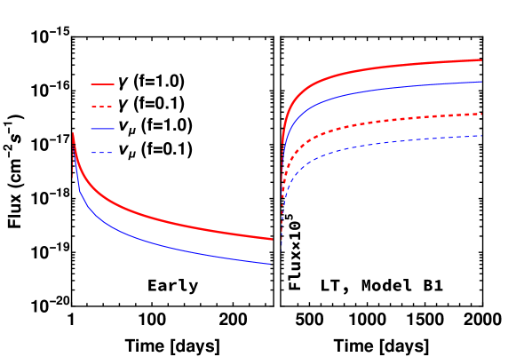
Figure 1: Temporal evolution of the flux of muon neutrinos (thin blue) and gamma-rays (thick red) at Earth from SN Model B1 (see also Table 1). The left plot extends up to $250$ days and it shows the early emission from SN Ib/c; the right panel shows the LT emission, i.e. beyond $250$ days. The y-axis of the right panel is rescaled by a factor $10^{5}$ at $250$ days. The continuous and dashed line styles represent the minimum ($f=1$) and maximum ($f=0.1$) CSM asymmetry, respectively. Note that the gamma-ray distributions do not take into account absorption. One can see that the early time emission from SNe Ib/c is significantly smaller than the corresponding LT emission. The other SN models (A and B2) show a similar temporal evolution and are therefore not shown.

Figure 1 shows the temporal evolution of the flux of gamma-rays (thick red) and muon neutrinos (thin blue) at Earth for SN Model B1 ($r^{-1.5}$ profile). The continuous and dashed lines show the cases of minimum ($f=1$) and maximum ($f=0.1$) asymmetry of the CSM, respectively [16]. The initial emission (up to $250$ days, left panel) is small as the CSM for SNe Ib/c is thin [32, 31]. The sharp rise (note the re-scaling of the y-axis at $250$ days, right panel) in the gamma-ray and neutrino spectra is due to the dense H-rich CSM. These fluxes are computed up to $2000$ days that correspond to the outer radius $r_{\rm o}$ of the CSM.

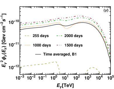
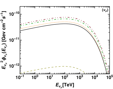
Figure 2: Top: Time snapshots of gamma-ray (on the left) and muon neutrino (on the right) fluxes as functions of the energy for SN Model B1 (see Table 1 for more details on the model parameters). The different curves indicate the flux at $255$, $1000$, $1500$, and $2000$ days. We consider the asymmetry factor to be $f=0.5$ to describe the typical spectral variation over the late emission phase. After the onset of the LT interaction, the fluxes increase with time. The fluxes averaged over $2000$ days has also been shown by the black curves. The gamma-ray fluxes between $1$–$10^{3}$ TeV are attenuated by pair production on the SN thermal photons. The amount of absorption is initially large, but it becomes smaller with time as the thermal photon density falls rapidly with the radius. Bottom: The fluxes of gamma-rays (left) and neutrinos (right) averaged over $2000$ days for Model A (medium thick), B1 (thinnest), and B2 (thickest) are shown for guidance.

The energy fluxes for SN Model B1, plotted in the top panel of Fig. 2 for gamma-rays (on the left) and muon neutrinos (on the right), reveal the dependence of the production mechanism on the SN model parameters. The curves in different colors and line styles represent fluxes at different time snapshots ($255$, $1000$, $1500$, and $2000$ days), highlighting the flux variation over the LT phase. This panel also shows the flux averaged over $2000$ days (black curve). Contrasting the flux at $255$ days (corresponding to the onset of the shock-CSM interaction) with the one above $1000$ days, one can see that the flux tends to increase with time. The maximum proton energy, $E_{\rm p,max}(r)$, fixes the spectral shape at higher energies as it acts as an exponential cut-off (see Sec. III). Hence, the fluxes of both gamma-rays and neutrinos fall rapidly above $10^{3}$ TeV.

The gamma-ray fluxes in the top left panel of Fig. 2 include absorption effects. In order to estimate the amount of absorption, the average energy and luminosity of thermal photons are assumed to be $0.05$ eV and $5\times 10^{40}~{}\rm erg/s$ [8, 6]. The gamma-ray fluxes show dips of different sizes due to pair production losses on the ambient thermal photons. The dips have different sizes as the optical depth $\tau_{loss}^{\rm S}(E_{\gamma}^{\prime},r)$ falls with the radius [32]; this implies that the gamma-rays produced at larger radii have smaller attenuation. However, the attenuation during propagation due to the EBL is not significant since SN 2014C is at $14.7$ Mpc [32]; therefore we neglect this effect.

The bottom panel of Figure 2 shows the fluxes averaged over $2000$ days for Model A, B1, and B2 (medium thick, thinnest and thickest, respectively). It is important to note that the fluxes for Model B depend on the CSM asymmetry factor $f$. The spectral shape remains the same for different $f$, but the normalization changes. For example, if we increase $f$ to 1, the time-averaged flux of Model B1 would be larger than the ones of the other CSM models. Note that the time-averaged fluxes of gamma-rays and neutrinos (black curves) are smaller than the maximum fluxes (at $2000$ days) by a few factors. Hence, in the following, we consider the time-averaged fluxes to be conservative estimates of the detection prospects of SN 2014C-like events.

V Detection prospects for SN 2014C-like bursts

In this section, we explore the detection prospects of gamma-rays and neutrinos from SNe Ib/c LT with current and upcoming gamma-ray (Fermi-LAT and CTA) and high energy neutrino (IceCube and IceCube-Gen2) detectors [60, 61, 62, 63, 64]. For comparison, we consider Model B1 and Model B2 with CSM asymmetry $f=0.5$.

V.1 Current and future detection prospects

The left (right) panel of Fig. 3 shows the gamma-ray (neutrino) flux for different models of the CSM, as well as the detection sensitivity of gamma-ray (neutrino) telescopes. The sensitivity curves of Fermi-LAT and CTA shown in the left panel correspond to $4$ years and $50$ hours of observation time, respectively. Whereas we show the $6$ year sensitivities of the neutrino detectors in the right panel. The SN model parameters are plagued by various uncertainties. In order to take this into account, we consider a range of variability for the microphysical parameters that contribute to the largest uncertainty in the expected fluxes; we take $\alpha$, $\epsilon_{\rm p}$ and $\epsilon_{\rm B}$ to vary in the range $2.0$–$2.2$, $10^{-2}$–$10^{-1}$ and $10^{-3}$–$10^{-2}$, respectively [5, 6, 34, 32]. The shaded bands in both panels of Fig. 3 also take into account the uncertainties on the CSM profile and the asymmetry factor $f$. Note that the conventional wind profile ($r^{-2}$) with our benchmark parameters (Table 1) leads to fluxes similar to the ones of Model B1 with $f=0.5$ [32].

While the detection prospects are less optimistic for Fermi-LAT, CTA may detect gamma-rays, if the CSM has a smaller asymmetry (i.e., $f\geq 0.5$) compared to the asymmetry for $f=0.5$. On the other hand, the non-detection of gamma-rays with CTA may contribute to constrain the CSM asymmetry factor $f$. The forecasted neutrino flux is beyond reach for IceCube (6 years with 90% confidence level (CL), [61]), in agreement with the fact that SN 2014C was not detected in neutrinos—see e.g. Ref. [65]. However, IceCube-Gen2 (6 years with 90% CL [62]) will have a better sensitivity and be closest to the predicted flux. For bursts occurring at closer distances than 15 Mpc, IceCube-Gen2 will have a reasonable prospect of detection. Interestingly, KM3NeT/ARCA (10 years with 90% CL, [64]) is expected to hold similar sensitivity as IceCube-Gen2 (6 years with 90% CL, [62]) and may probe similar SNe Ib/c LT objects. However, due to the limited availability of the KM3NeT/ARCA sensitivity for the energy bins over the point source observation time, it is difficult to make a precise estimate of the detector response and therefore we choose to do not explicitly show the detection prospects of KM3NeT/ARCA in Fig. 3. Also, any comparison of the detector sensitivities with the predicted neutrino fluxes only provides a broad idea about the detection prospects. This is because of the different sensitivities at different energy bins [66, 61]. For a robust forecast, one should compute the number of events considering the impact of the backgrounds. Since our neutrino flux prediction has large astrophysical uncertainties, we only investigate the differential flux sensitivities of the detector to give an idea of the detection prospects.

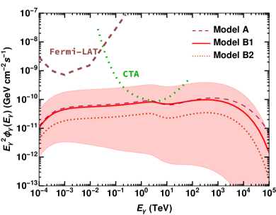
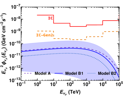
Figure 3: Left: Time averaged gamma-ray flux for different CSM models (see Table 1). The red band represents the time-averaged flux of SN Ib/c LT obtained considering the uncertainties in the model parameters ($\epsilon_{P}\sim 10^{-2}$–$10^{-1}$, $\epsilon_{B}\sim 10^{-3}$–$10^{-2}$ and $f\sim 0.1$–$1$), while the other model parameters are kept fixed as detailed in Table 1. The uncertainty band as been obtained as follows: for the upper limit, we take $\alpha=2.0$, $\epsilon_{\rm p}=10^{-1}$, $\epsilon_{\rm B}=10^{-2}$ and $f=1$ for Model B1; for the lower limit, we choose $\alpha=2.0$, $\epsilon_{\rm p}=10^{-2}$, $\epsilon_{\rm B}=10^{-3}$, and $f=0.1$ for Model B2. The red continuous and dotted curves show the fluxes for Model B1 and Model B2, respectively, for $f=0.5$. The pink dashed curve represents the flux for Model A. The sensitivities of Fermi-LAT (4 years) and CTA (50 hours) are plotted in brown and green, respectively. CTA may be able to detect gamma-rays from SNe closer than $\simeq 15$ Mpc. Right: Corresponding neutrino flux and sensitivities of IceCube (6 years with $90\%$ CL) [61], IceCube-Gen2 (6 years with $90\%$ CL) [62]. The blue band represents the uncertainty in the model parameters. The sensitivity chosen for IceCube corresponds to the one at the declination of $0^{\circ}$ where IceCube is most sensitive. Neutrinos from SNe Ib/c LT may be detectable for bursts occurring closer than $15$ Mpc.

The secondary fluxes for the asymmetric CSM models are computed by assuming that the disk (which gives rise to the asymmetry in the CSM) is aligned with the observer’s line of sight. When the disk is not along the line of sight, the fluxes might be smaller than the ones shown in Fig. 3. However, this uncertainty lies within the uncertainty bands shown in Fig. 3.

V.2 Detection horizon

The detection prospects of SNe with LT emission depend on the rate of such events. In the local universe, we expect about $26\%$ SNe Ib/c [20], of these about $10\%$ should be Ib/c LT [6]. Thus, the local rate of SNe Ib/c LT is about $2.6\%$ of the local core collapse SN rate ($1.25\pm 0.5\times 10^{-4}~{}\rm Mpc^{-3}yr^{-1}$ [67]).

To investigate upcoming detection prospects, we consider SN 2014C as the benchmark SN Ib/c LT (Table 1, third column) and calculate the SN detection horizon defined as the distance at which the source should be located, for which the energy integrated flux (averaged over $2000$ days) falls below the telescope sensitivity. The energy range for these integrated fluxes is optimized according to the telescope sensitivity. For Fermi-LAT and CTA, we consider $10^{-4}$–$10^{-2}$ TeV and $5\times 10^{-2}$–$5\times 10^{1}$ TeV respectively, whereas we focus on $10^{2}$–$10^{4}$ TeV for the neutrino telescopes. Note that the sensitivity for the neutrino telescopes depends on the declination [60, 61, 62]. Hence, unlike the gamma-ray telescopes, we consider a maximum and minimum sensitivity resulting in a band.

Figure 4 shows the detection horizon for gamma-rays (left) and neutrinos (right). The left panel only shows the detection horizon of CTA; Fermi-LAT is not shown because of its weak sensitivity and different energy range compared to CTA (see Fig. 3). The gamma-ray fluxes for Model B1 and Model B2 are represented by red continuous and dotted curves respectively, while the pink dashed line shows the flux for Model A. The shaded bands in both panels correspond to the uncertainty in the parameters ($\alpha\in[2.0-2.2]$, $\epsilon_{P}\in[10^{-2},10^{-1}]$ and $\epsilon_{B}\in[10^{-3},10^{-2}]$) and CSM asymmetry factor ($f\in[0.1,1]$) as in Fig. 3. The horizontal dotted line represents the sensitivity of CTA. The detection horizon for CTA extends up to $10$ Mpc, while the detection horizon of Fermi-LAT is limited to $4$ Mpc (results not shown here). Interestingly, the density profile of the CSM for SN (Model B1 and Model B2) plays an important role in the detectability of such SNe. For example, the detection horizon of CTA is about $10$ Mpc for Model B1 and about $6$ Mpc for Model B2.

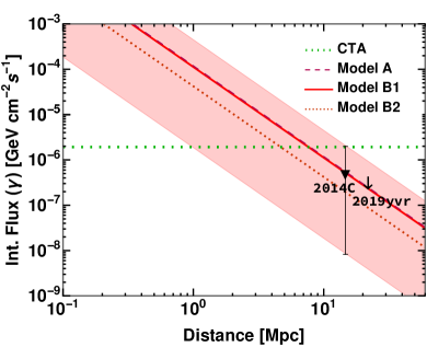
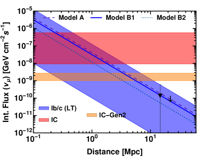
Figure 4: Left: Detection horizon (see main text for details) in gamma-rays for SNe Ib/c LT. The time-averaged gamma-ray flux has been integrated over energy in the range $5\times 10^{-2}$–$5\times 10^{1}$ TeV for SN Model B1 (red) and Modlel B2 (red dotted) for an asymmetry factor $f=0.5$. The pink dashed line represents the flux for SN Model A, slightly overlapping with the SN Model B1 flux. The red band corresponds to the uncertainties in the parameters $\alpha\in[2.0-2.2]$, and $\epsilon_{P}\in[10^{-2},10^{-1}]$ and $\epsilon_{B}\in[10^{-3},10^{-2}]$, and $f\in[0.1,1]$. The horizontal dotted line represents the CTA sensitivity. The detection horizon is about $10$ Mpc. Right: Corresponding detection horizon for neutrinos. The blue band represents the time-averaged flux integrated in the range $10^{2}$–$10^{4}$ TeV. The purple dashed, blue and light blue dotted lines show the fluxes for the SN Model A, Model B1 and Model B2 respectively. The $90\%$ CL sensitivity bands of different detectors are obtained by considering the variation of the declination angle ($\delta$) of the source. The band for IceCube corresponds to the minimum detector sensitivity for $\delta=-60^{\circ}$ [60] and maximum detector sensitivity, $\delta=0^{\circ}$ [61]. Similarly, we consider $\delta=30^{\circ}$ (minimum) and $\delta=0^{\circ}$ (maximum) for IceCube-Gen2 [62]; IceCube-Gen2 has the potential to detect SNe Ib/c LT up to $10$ Mpc, while IceCube can only probe SNe up to $3$ Mpc. For guidance, the black data points in both panels show the fluxes of recent nearby SN Ib/c LTe: SN 2014C and SN 2019yvr.

The detection horizons of current and upcoming neutrino telescopes are shown in the right panel of Fig. 4. The blue continuous and light-blue dotted lines show the integrated $\nu_{\mu}$ flux as a function of the SN distance (Mpc) for SN Model B1 and Model B2, respectively, and the purple dashed line corresponds to Model A. The blue band takes into account the model uncertainties ( $\alpha$, $\epsilon_{\rm p},~{}\epsilon_{\rm B},~{}f$). The upper and lower limits of the sensitivity of neutrino telescopes depend on the SN declination angle and are shown as bands in Fig. 4. The most optimistic model prediction (upper limit of blue band) and most sensitive future telescopes (lower limit of orange and green bands) combination imply that SNe Ib/c LT may be detected up to $10$ Mpc with IceCube-Gen2. On the other hand, the detection horizon of IceCube (red band) is limited to about $4$ Mpc.

For guidance, we also show in Fig. 4 the gamma-ray and muon neutrino fluxes of SN 2014C that occurred at $14.7$ Mpc as well as the ones of SN 2019yvr observed at $22$ Mpc [18]. The flux of SN 2014C (black inverted triangle) is obtained by relying on the same parameters as the ones of the blue line. As for SN 2019yvr, we have chosen $r_{\rm i}=3\times 10^{16}~{}\rm cm$ [68, 18], $\epsilon_{\rm p}=0.1$, and $\epsilon_{\rm B}=0.01$ to compute the flux upper limits. The other parameters for SN 2019yvr are the same as in Table 1, due to limited information otherwise available for them. Both these events lie beyond the detection horizon of gamma-ray and neutrino telescopes. These findings are in agreement with the non-observation of neutrinos with IceCube and gamma-rays with Fermi-LAT from SN 2014C and SN 2019yvr. Similar LT shock-CSM interaction has been observed in other SNe Ib/c, such as SN 2003gk (estimated distance: $45$ Mpc [69]), SN 2004dk (estimated distance: $21.05$ Mpc [17]), SN 2004cc (estimated distance: $18$ Mpc [70]), and SN 2004gq (estimated distance: $26$ Mpc [70]). Due to their larger or comparable distances, we do not include them in Fig. 4, since we expect comparable or worse detection prospects.

In Ref. [32], the discovery horizon of IceCube-Gen2 for SN 2014C-like events was found to be about $6$ Mpc. However, here we report a detection horizon of $10$ Mpc. This is because the results in Ref. [32] were based on a wind-like CSM profile ($r^{-2}$) whereas we consider different CSM profiles in this paper (see Sec. II). In addition, the sensitivity of IceCube-Gen2 corresponding to $5\sigma$ CL considered in Ref. [32] is smaller than the $90\%$ CL sensitivity considered in this work. This also holds for the detection horizons of IceCube. The discovery horizon of CTA for SN 2014C-like events was found to be about $2$–$6$ Mpc in Ref. [34] depending on the energy of gamma-rays and considering the SN emission up to $396$ days, for a dense wind-like CSM [6]. These conclusions are in agreement with our findings.

VI Conclusions

Late X-ray data of some SNe of Type Ib/c, such as SN 2014C, have revealed the presence of a dense hydrogen rich CSM far away from the stellar core, whose origin is not yet well understood and still subject of investigation. High energy protons accelerated in the SN shock and interacting with the CSM can lead to the production of secondary particles, such as gamma-rays and high energy neutrinos. Yet, the emission of these high energy particles strongly depends on the efficiency of the acceleration mechanism. The acceleration efficiency would be suppressed if the shock-CSM interaction fails to produce sufficient turbulence and magnetic field amplification. Hence, it is crucial to look for neutrino and gamma-ray signals to assess the acceleration efficiency.

In this paper, we have computed the fluxes of gamma-rays and high energy neutrinos from SNe Ib/c LT, considering SN 2014C as the prototype SNe Ib/c with LT emission. Because of the uncertainties related to the properties of the CSM, we have considered three different CSM models: Model A (symmetric, $r^{-2.5}$), Model B1 (asymmetric, $r^{-1.5}$) and Model B2 (asymmetric, $r^{-2.4}$). According to the CSM profile, we predict a range of variability for the expected fluxes of neutrinos and gamma-rays.

Based on the observation of SN 2014C and the uncertainties in the model parameters, we have investigated present and future detection prospects of SNe Ib/c LT in neutrinos and gamma-rays. We find that the detection horizon for Fermi-LAT and CTA is $4$ Mpc and $10$ Mpc, respectively. Similarly, for neutrinos, the detection horizon of IceCube is about $4$ Mpc, while IceCube-Gen2 can potentially detect SNe Ib/c LT up to $10$ Mpc. However, the detection horizon in neutrinos can vary up to a few Mpc depending on the source declination, because of the related neutrino telescope sensitivity. The highly symmetric CSM models are found to have the best detection prospects while increasing the asymmetry in the CSM worsens the detection prospects. Our findings are in agreement with the non-detection of gamma-rays and neutrinos from SN 2014C and SN 2019yvr and other SN bursts with LT emission occurring at larger distances. Yet, upcoming detection of neutrinos and gamma-rays from local SNe Ib/c LT will be crucial to probe the CSM properties and the nature of such transients.

The modeling of the gamma-ray and neutrino emission from SNe Ib/c LT presented in this work is based on the observations of SN 2014C. Considering the frequency of SN 2014C-like events in the recent past, one might expect to shed light on the properties of the CSM of SNe Ib/c exhibiting LT emission with upcoming radio and X-ray observations. In addition, future gamma-ray and neutrino telescopes will provide complementary information, if SN bursts with LT emission should occur within $15$ Mpc.

Appendix A Timescales for proton acceleration and different cooling processes

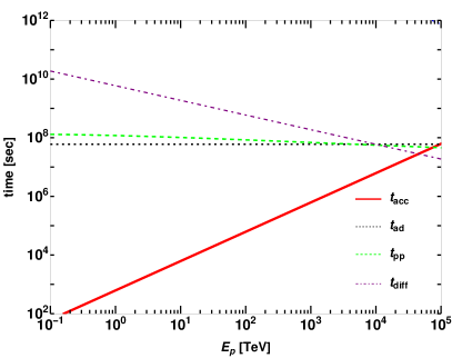
Figure 5: Acceleration time scale versus different cooling timescales.

Protons that undergo shock acceleration experience energy losses through various mechanisms. In this Appendix, we present a quantitative estimate of these timescales to show the efficiency of proton acceleration.

The expressions for the acceleration timescale as well as different cooling timescales ($pp$ interaction, adiabatic and diffusion) are provided in Sec. III. In Fig. 5, we have plotted these timescales as a function of proton energy, $E_{\rm p}$ computed at the beginning of CSM interaction, i.e, at $r=r_{\rm i}$. This figure shows that all the loss timescales become comparable to the acceleration timescale above $10^{4}$ TeV. In addition to these losses, protons could also lose energy due to photopion production ($p\gamma$), Inverse Compton, Bethe-Heitler, synchrotron radiation. However, the timescales of these losses for the case of SN 2014C are found to be very large ($>10^{13}$ seconds), therefore we do not show them in this figure; see Ref. [32] for details. It can be clearly seen from this plot that the relevant loss timescales are long enough for the protons to efficiently accelerate to PeV energies.

References

- Smith et al. [2011] N. Smith, W. Li, A. V. Filippenko, and R. Chornock, Mon. Not. R. Astron. Soc. 412, 1522 (2011), arXiv:1006.3899 [astro-ph.HE] .
- Woosley et al. [2021] S. E. Woosley, T. Sukhbold, and D. N. Kasen, Astrophys. J. 913, 145 (2021), arXiv:2009.06868 [astro-ph.HE] .
- Immler et al. [2008] S. Immler, M. Modjaz, W. Landsman, F. Bufano, P. J. Brown, P. Milne, L. Dessart, S. T. Holland, M. Koss, D. Pooley, R. P. Kirshner, A. V. Filippenko, N. Panagia, R. A. Chevalier, P. A. Mazzali, N. Gehrels, R. Petre, D. N. Burrows, J. A. Nousek, P. W. A. Roming, E. Pian, A. M. Soderberg, and J. Greiner, Astrophys. J. Lett. 674, L85 (2008), arXiv:0712.3290 [astro-ph] .
- Foley et al. [2007] R. J. Foley, N. Smith, M. Ganeshalingam, W. Li, R. Chornock, and A. V. Filippenko, Astrophys. J. Lett. 657, L105 (2007), arXiv:astro-ph/0612711 [astro-ph] .
- Milisavljevic et al. [2015] D. Milisavljevic et al., Astrophys. J. 815, 120 (2015), arXiv:1511.01907 [astro-ph.HE] .
- Margutti et al. [2017] R. Margutti et al., Astrophys. J. 835, 140 (2017), arXiv:1601.06806 [astro-ph.HE] .
- Tinyanont et al. [2019] S. Tinyanont et al., Astrophys. J. 887, 75 (2019), arXiv:1909.06403 [astro-ph.SR] .
- Brethauer et al. [2020] D. Brethauer, R. Margutti, D. Milisavljevic, and M. Bietenholz, Res. Notes AAS 4, 235 (2020), arXiv:2012.04081 [astro-ph.HE] .
- Thomas et al. [2022] B. P. Thomas, J. C. Wheeler, V. V. Dwarkadas, C. Stockdale, J. Vinkó, D. Pooley, Y. Xu, G. Zeimann, and P. MacQueen, Astrophys. J. 930, 57 (2022), arXiv:2203.12747 [astro-ph.HE] .
- Zapartas et al. [2017] E. Zapartas et al., Astron. Astrophys. 601, A29 (2017), arXiv:1701.07032 [astro-ph.HE] .
- Vargas et al. [2022] F. Vargas, F. De Colle, D. Brethauer, R. Margutti, and C. G. Bernal, Astrophys. J. 930, 150 (2022), arXiv:2102.12581 [astro-ph.HE] .
- Smith [2014] N. Smith, Ann. Rev. Astron. Astrophys. 52, 487 (2014), arXiv:1402.1237 [astro-ph.SR] .
- Ofek et al. [2014a] E. O. Ofek et al., Astrophys. J. 781, 42 (2014a), arXiv:1307.2247 [astro-ph.HE] .
- Ofek et al. [2013] E. O. Ofek, L. Lin, C. Kouveliotou, G. Younes, E. Gogus, M. M. Kasliwal, and Y. Cao, Astrophys. J. 768, 47 (2013), arXiv:1303.3894 [astro-ph.HE] .
- Margutti et al. [2014] R. Margutti et al., Astrophys. J. 780, 21 (2014), arXiv:1306.0038 [astro-ph.HE] .
- Brethauer et al. [2022] D. Brethauer, R. Margutti, D. Milisavljevic, M. F. Bietenholz, R. Chornock, D. L. Coppejans, F. De Colle, A. Hajela, G. Terreran, F. Vargas, L. DeMarchi, C. Harris, W. V. Jacobson-Galán, A. Kamble, D. Patnaude, and M. C. Stroh, Astrophys. J. 939, 105 (2022), arXiv:2206.00842 [astro-ph.HE] .
- Mauerhan et al. [2018] J. C. Mauerhan, W. Zheng, T. Brink, M. L. Graham, I. Shivvers, K. Clubb, and A. V. Filippenko, Mon. Not. Roy. Astron. Soc. 478, 5050 (2018), arXiv:1803.07051 [astro-ph.SR] .
- Kilpatrick et al. [2021] C. D. Kilpatrick et al., Mon. Not. Roy. Astron. Soc. 504, 2073 (2021), arXiv:2101.03206 [astro-ph.HE] .
- Balasubramanian et al. [2021] A. Balasubramanian, A. Corsi, E. Polisensky, T. E. Clarke, and N. E. Kassim, Astrophys. J. 923, 32 (2021), arXiv:2101.07348 [astro-ph.HE] .
- Smith [2014] N. Smith, Ann. Rev. Astron. Astrophys. 52, 487 (2014), arXiv:1402.1237 [astro-ph.SR] .
- Kelner et al. [2006] S. R. Kelner, F. A. Aharonian, and V. V. Bugayov, Phys. Rev. D 74, 034018 (2006), [Erratum: Phys.Rev.D 79, 039901 (2009)], arXiv:astro-ph/0606058 .
- Marcowith et al. [2018] A. Marcowith, V. V. Dwarkadas, M. Renaud, V. Tatischeff, and G. Giacinti, Mon. Not. R. Astron. Soc. 479, 4470 (2018), arXiv:1806.09700 [astro-ph.HE] .
- Marcowith et al. [2014] A. Marcowith, M. Renaud, V. Dwarkadas, and V. Tatischeff, Nuc. Phys. B Proc. Suppl. 256, 94 (2014), arXiv:1409.3670 [astro-ph.HE] .
- Cristofari et al. [2022] P. Cristofari, A. Marcowith, M. Renaud, V. V. Dwarkadas, V. Tatischeff, G. Giacinti, E. Peretti, and H. Sol, Mon. Not. R. Astron. Soc. 511, 3321 (2022), arXiv:2201.09583 [astro-ph.HE] .
- Wang et al. [2019] K. Wang, T.-Q. Huang, and Z. Li, Astrophys. J. 872, 157 (2019), arXiv:1901.05598 [astro-ph.HE] .
- Murase et al. [2011] K. Murase, T. A. Thompson, B. C. Lacki, and J. F. Beacom, Phys. Rev. D 84, 043003 (2011), arXiv:1012.2834 [astro-ph.HE] .
- Murase et al. [2014] K. Murase, T. A. Thompson, and E. O. Ofek, Mon. Not. R. Astron. Soc. 440, 2528 (2014), arXiv:1311.6778 [astro-ph.HE] .
- Murase et al. [2013] K. Murase, M. Ahlers, and B. C. Lacki, Phys. Rev. D 88, 121301 (2013), arXiv:1306.3417 [astro-ph.HE] .
- Sarmah et al. [2023] P. Sarmah, S. Chakraborty, and J. C. Joshi, Mon. Not. R. Astron. Soc. 521, 1144 (2023), arXiv:2301.04161 [astro-ph.HE] .
- Kheirandish and Murase [2022] A. Kheirandish and K. Murase, (2022), arXiv:2204.08518 [astro-ph.HE] .
- Murase [2018] K. Murase, Phys. Rev. D 97, 081301 (2018), arXiv:1705.04750 [astro-ph.HE] .
- Sarmah et al. [2022] P. Sarmah, S. Chakraborty, I. Tamborra, and K. Auchettl, JCAP 2022, 011 (2022), arXiv:2204.03663 [astro-ph.HE] .
- Stasik [2018] A. Stasik, Search for High Energetic Neutrinos from Core Collapse Supernovae using the IceCube Neutrino Telescope, Ph.D. thesis (2018).
- Murase et al. [2019] K. Murase, A. Franckowiak, K. Maeda, R. Margutti, and J. F. Beacom, Astrophys. J. 874, 80 (2019), arXiv:1807.01460 [astro-ph.HE] .
- Quataert and Shiode [2012] E. Quataert and J. Shiode, Mon. Not. R. Astron. Soc. 423, L92 (2012), arXiv:1202.5036 [astro-ph.SR] .
- Chevalier [1982] R. A. Chevalier, Astrophys. J. 258, 790 (1982).
- Mastichiadis [1996] A. Mastichiadis, aap 305, L53 (1996), arXiv:astro-ph/9601132 [astro-ph] .
- Petropoulou et al. [2016] M. Petropoulou, A. Kamble, and L. Sironi, Mon. Not. Roy. Astron. Soc. 460, 44 (2016), arXiv:1603.00891 [astro-ph.HE] .
- Ofek et al. [2014b] E. O. Ofek et al., Astrophys. J. 788, 154 (2014b), arXiv:1404.4085 [astro-ph.HE] .
- Petropoulou et al. [2017] M. Petropoulou, S. Coenders, G. Vasilopoulos, A. Kamble, and L. Sironi, Mon. Not. Roy. Astron. Soc. 470, 1881 (2017), arXiv:1705.06752 [astro-ph.HE] .
- Blasi [2013] P. Blasi, Astron. Astrophys. Rev. 21, 70 (2013), arXiv:1311.7346 [astro-ph.HE] .
- Malkov and Drury [2001] M. A. Malkov and L. O. Drury, Reports on Progress in Physics 64, 429 (2001).
- Blandford and Eichler [1987] R. Blandford and D. Eichler, physrep 154, 1 (1987).
- Cardillo et al. [2015] M. Cardillo, E. Amato, and P. Blasi, Astropart. Phys. 69, 1 (2015), arXiv:1503.03001 [astro-ph.HE] .
- Cristofari et al. [2022] P. Cristofari, P. Blasi, and D. Caprioli, Astrophys. J. 930, 28 (2022), arXiv:2203.15624 [astro-ph.HE] .
- Murase et al. [2015] K. Murase, K. Kashiyama, K. Kiuchi, and I. Bartos, Astrophys. J. 805, 82 (2015), arXiv:1411.0619 [astro-ph.HE] .
- Bell [2004] A. R. Bell, Monthly Notices of the Royal Astronomical Society 353, 550 (2004), https://academic.oup.com/mnras/article-pdf/353/2/550/3869038/353-2-550.pdf .
- Bell [2005] A. R. Bell, Monthly Notices of the Royal Astronomical Society 358, 181 (2005), https://academic.oup.com/mnras/article-pdf/358/1/181/3479398/358-1-181.pdf .
- Lucek and Bell [2000] S. G. Lucek and A. R. Bell, Monthly Notices of the Royal Astronomical Society 314, 65 (2000), https://academic.oup.com/mnras/article-pdf/314/1/65/3566804/314-1-65.pdf .
- Schure and Bell [2013] K. M. Schure and A. R. Bell, Monthly Notices of the Royal Astronomical Society 435, 1174 (2013), https://academic.oup.com/mnras/article-pdf/435/2/1174/3490642/stt1371.pdf .
- Bell et al. [2013] A. R. Bell, K. M. Schure, B. Reville, and G. Giacinti, Monthly Notices of the Royal Astronomical Society 431, 415 (2013), https://academic.oup.com/mnras/article-pdf/431/1/415/18243010/stt179.pdf .
- Stroh et al. [2021] M. C. Stroh, G. Terreran, D. L. Coppejans, J. S. Bright, R. Margutti, M. F. Bietenholz, F. De Colle, L. DeMarchi, R. B. Duran, D. Milisavljevic, K. Murase, K. Paterson, and W. L. Williams, Astrophys. J. 923, L24 (2021), arXiv:2106.09737 [astro-ph.HE] .
- Murase et al. [2011] K. Murase, T. A. Thompson, B. C. Lacki, and J. F. Beacom, Phys. Rev. D 84, 043003 (2011), arXiv:1012.2834 [astro-ph.HE] .
- Katz et al. [2012] B. Katz, N. Sapir, and E. Waxman, in Death of Massive Stars: Supernovae and Gamma-Ray Bursts, Vol. 279, edited by P. Roming, N. Kawai, and E. Pian (2012) pp. 274–281, arXiv:1106.1898 [astro-ph.HE] .
- Sarmah et al. [2022] P. Sarmah, S. Chakraborty, I. Tamborra, and K. Auchettl, (2022), arXiv:2204.03663 [astro-ph.HE] .
- Celli et al. [2019] S. Celli, G. Morlino, S. Gabici, and F. A. Aharonian, Mon. Not. Roy. Astron. Soc. 490, 4317 (2019), arXiv:1906.09454 [astro-ph.HE] .
- Metzger et al. [2016] B. D. Metzger, D. Caprioli, I. Vurm, A. M. Beloborodov, I. Bartos, and A. Vlasov, Monthly Notices of the Royal Astronomical Society 457, 1786 (2016), https://academic.oup.com/mnras/article-pdf/457/2/1786/2926159/stw123.pdf .
- Ahlers and Murase [2014] M. Ahlers and K. Murase, Phys. Rev. D 90, 023010 (2014).
- [59] “Centre de Données Astronomiques de Strasbourg,” https://cds.u-strasbg.fr/, accessed: 2010-09-30.
- Aartsen et al. [2017] M. G. Aartsen et al. (IceCube), Astrophys. J. 835, 151 (2017), arXiv:1609.04981 [astro-ph.HE] .
- Aartsen et al. [2019] M. G. Aartsen et al. (IceCube), Eur. Phys. J. C 79, 234 (2019), arXiv:1811.07979 [hep-ph] .
- Aartsen et al. [2021] M. G. Aartsen et al. (IceCube-Gen2), J. Phys. G 48, 060501 (2021), arXiv:2008.04323 [astro-ph.HE] .
- Aiello et al. [2019] S. Aiello et al. (KM3NeT), Astropart. Phys. 111, 100 (2019), arXiv:1810.08499 [astro-ph.HE] .
- Ambrogi et al. [2018] L. Ambrogi, S. Celli, and F. Aharonian, Astropart. Phys. 100, 69 (2018), arXiv:1803.03565 [astro-ph.HE] .
- Abbasi et al. [2023] R. Abbasi et al., (2023), arXiv:2303.03316 [astro-ph.HE] .
- Abbasi and et al. IceCube Collaboration [2011] R. Abbasi and et al. IceCube Collaboration, Astrophys. J. 732, 18 (2011), arXiv:1012.2137 [astro-ph.HE] .
- Lien et al. [2010] A. Lien, B. D. Fields, and J. F. Beacom, Phys. Rev. D 81, 083001 (2010), arXiv:1001.3678 [astro-ph.CO] .
- Sun et al. [2022] N.-C. Sun, J. R. Maund, P. A. Crowther, R. Hirai, A. Kashapov, J.-F. Liu, L.-D. Liu, and E. Zapartas, Mon. Not. R. Astron. Soc. 510, 3701 (2022).
- Bietenholz et al. [2014] M. F. Bietenholz, F. De Colle, J. Granot, N. Bartel, and A. M. Soderberg, Mon. Not. R. Astron. Soc. 440, 821 (2014), arXiv:1310.7171 [astro-ph.HE] .
- Wellons et al. [2012] S. Wellons, A. M. Soderberg, and R. A. Chevalier, Astrophys. J. 752, 17 (2012), arXiv:1201.5120 [astro-ph.HE] .