Inheriting Bayer’s Legacy: Joint Remosaicing and Denoising for Quad Bayer Image Sensor

Abstract

Pixel binning based Quad sensors have emerged as a promising solution to overcome the hardware limitations of compact cameras in low-light imaging. However, binning results in lower spatial resolution and non-Bayer CFA artifacts. To address these challenges, we propose a dual-head joint remosaicing and denoising network (DJRD), which enables the conversion of noisy Quad Bayer and standard noise-free Bayer pattern without any resolution loss. DJRD includes a newly designed Quad Bayer remosaicing (QB-Re) block, integrated denoising modules based on Swin-transformer and multi-scale wavelet transform. The QB-Re block constructs the convolution kernel based on the CFA pattern to achieve a periodic color distribution in the perceptual field, which is used to extract exact spectral information and reduce color misalignment. The integrated Swin-Transformer and multi-scale wavelet transform capture non-local dependencies, frequency and location information to effectively reduce practical noise. By identifying challenging patches utilizing Moiré and zipper detection metrics, we enable our model to concentrate on difficult patches during the post-training phase, which enhances the model’s performance in hard cases. Our proposed model outperforms competing models by approximately 3dB, without additional complexity in hardware or software.

1 Introduction

In recent years, smartphones have emerged as the most popular choice for photography. Nevertheless, due to the demand for portable devices, smartphones are designed with compact and cost-efficient cameras, which pose a challenge in capturing high-quality images comparable to those produced by DSLR cameras [14].

Figure 1: To address the raw Quad Bayer demosaicing problem, previous methods mainly focus on models demosaic the Quad directly or average the neighbor $2\times 2$ pixels to one, while we promote a novel view by designing a joint but flexible remosaic and denoise module to convert noisy Quad Bayer to full-resolution clean Bayer. It allows any advance in Bayer CFA tools to be directly applicable in Quad Bayer.

Pixel binning using Quad Bayer Color Filter Array (CFA) technology has been recognized as a promising approach for producing high-quality images under low-light conditions, as evidenced in previous studies [37, 17]. The Quad Bayer CFA pattern is composed of periodic $2\times 2$ cells that are designed to capture two consecutive homogenous pixels of the same color in two spatial dimensions. By averaging four pixels within a $2\times 2$ neighborhood, the Quad Bayer CFA can capture larger pixels and collect twice as much light intensity as the standard Bayer pattern, resulting in high-sensitivity and high-resolution imaging with low energy consumption.

Apart from improving image quality in low-light conditions, the Quad Bayer CFA also enables original equipment manufacturers (OEMs) to create higher-resolution sensors for mobile photographers [16, 1]. This feature makes it possible to produce high-resolution videos, such as 8K videos, which allow for high-definition imaging even when using digital zoom on smartphones. Therefore, the Quad Bayer CFA is commonly used in smartphone cameras. For example, leading mobile companies have utilized Quad Bayer CFA in conjunction with 108-megapixel image sensors in their latest flagship smartphones, e.g., iPhone 14 Pro, providing a versatile photography experience for enthusiastic mobile photographers [30], as shown in Fig. 2.

Reconstructing RGB image from raw Quad Bayer mosaic can be achieved by averaging the $2\times 2$ neighboring pixels and applying a demosaicing algorithm designed for the Bayer CFA. However, this approach involves downsampling the Quad Bayer to Bayer, leading to a quarter of the original image resolution, as depicted in Fig. 1. An alternative approach is Quad Bayer demosaicing, which aims to directly generate RGB images from raw Quad Bayer data, as demonstrated in previous works [1, 30]. Nevertheless, demosaicing on Quad Bayer data often produces visual artifacts due to the six color components of the Quad Bayer CFA being located differently than the three color components of the standard Bayer CFA [15]. This also implies that Quad Bayer CFA is more susceptible to aliasing compared to Bayer CFA during demosaicing. In addition, even with a reliable Quad Bayer demosaicing algorithm, it is necessary to redesign the current sophisticated Bayer image signal processor (ISP) for Quad sensor with new arrangement of color components in both software and hardware.

Against the above issues, we propose a dual-head joint remosaicing and denoising network, which enables conversion of noisy Quad Bayer to a standard clean Bayer mosaic without any loss in resolution. It facilitates the use of all the software and hardware designed for classic Bayer CFA, and allows any advance in Bayer CFA tools to be directly applicable in our approach. Therefore, the impact is far-reaching, extending beyond just remosaicing.

Firstly, we propose a novel and efficient basic component, the Quad Bayer remosaicing (QB-Re) block, which utilizes Quad Bayer CFA guided convolution to extract spectral information and reduce color misalignment. This design constructs the convolution kernel based on the CFA pattern, with the same weights assigned to pixels in the same relative positions within the CFA, and periodic weight changes as the kernel slides. This results in a periodic color distribution in the perceptual field, ensuring that neighboring pixels with the same color have similar spectral distributions. Additionally, we introduce a Quad Bayer CFA pooling layer that refines features with the same relative CFA position, instead of using common pooling methods.

Secondly, based on the proposed QB-Re block, we present a dual-head joint remosaicing and denoising network, named DJRD. It leverages the Swin-Transformer and multi-scale wavelet transform to model non-local dependencies, while simultaneously capturing frequency and location information of feature maps with limited computation. Thirdly, to make the DJRD model more robust and better suited for practical scenarios, in the post-training phase, we fine-tune our DJRD on difficult image patches. These patches were selected using hard patch detection metrics, which helped identify regions where the model was struggling to make accurate predictions. Overall, our contributions are four-fold:

• We propose DJRD, a novel dual-head joint remosaicing and denoising network to reconstruct clean classic Bayer images from noisy Quad Bayer mosaic without any resolution loss.

• We present a Quad Bayer CFA-driven CNN architecture to exploit the spatial-channel correlation of Quad Bayer.

• We enhance DJRD’s capability in challenging scenarios through fine-tuning it on difficult cases by using hard patches finding metrics.

• Extensive experiments show that DJRD establishes new state-of-the-arts on various datasets for joint Quad Bayer remosaicing and denoising task.

2 Related Work

2.1 Classic Bayer Demosaicing

Bayer demosaicing is a low-level image signal processing (ISP) task that has been extensively researched for several decades. The main objective of demosaicing is to reconstruct RGB images from observed mosaic images captured by a sensor with a Bayer filter. Interpolation-based methods are commonly employed to demosaic R, G, and B channels by using various linear or non-linear interpolation techniques, such as bilinear interpolation [25], directional linear [40], and others. Although these methods are spatially invariant and effective for a single color channel, they can produce pseudocolor at joints with different color variations. To overcome this color issue, several demosaicing methods have been developed, such as the edge-adaptive algorithm [34], reconstruction-based models [28], and frequency domain filtering [38, 8]. However, these conventional models still have limitations, such as visually disturbing artifacts like moiré patterns appearing on challenging high-pass regions when enlarging the local patches [21]. Recently, deep learning-based methods have been proposed and shown superior performance on various image processing tasks, including demosaicing, e.g., [21, 32, 33, 10, 31, 42, 24, 27, 2, 7]. These methods utilize deep neural networks to learn a mapping between observed mosaic images and their corresponding RGB images, achieving promising performance.

2.2 Joint Demosaicing and Denoising

Bayer demosaicing is a widely researched topic in the field of imaging. However, real-world raw images are often corrupted by various types of noise due to hardware limitations and environmental factors [21, 1, 20], among others. Therefore, demosaicing algorithms that are solely designed for this task cannot be directly applied to real scenes. To overcome this issue, hybrid solution frameworks for image processing have been proposed that simultaneously address both denoising and demosaicing [35, 19, 9, 6, 12]. By considering more realistic noise factors in the imaging process, these joint denoising and demosaicing methods reduce error accumulation caused by the distributed execution of each image signal processor (ISP) and thus achieve relatively better performance on real data compared to models that process mosaics independently.

2.3 Non-Bayer Demosaicing

In recent years, deep learning techniques have been employed for demosaicing of Bayer pattern images. However, the use of Quad Bayer technology in cellphone cameras is a relatively new development, and there have been few studies on dedicated Quad Bayer demosaicing, either using traditional or deep learning approaches. Two recent works, namely PIPNet [1] and SAGAN [30], have focused on Quad Bayer demosaicing. These methods employ depth-spatial feature attention and adversarial spatial-asymmetric attention, respectively, to perform demosaicing directly on the Quad Bayer raw images. In both methods, missing pixels are reconstructed using a deep neural network that leverages intra-channel and inter-channel correlations in the raw image.

Figure 2: Quad Bayer and Bayer Color Filter Array (CFA) layouts, the pictures captured by image sensor with Bayer structure and image sensor with Quad Bayer structure (Sony IMX689). One can see that Quad Bayer prevents resolution loss in a low-illuminance environment and produces low-noise nightscape photo. Please zoom in for better view.

Figure 3: Overview of the proposed dual-head joint remosaicing and denoising network (DJRD) for Quad Bayer CFA based image sensor.

3 Problem Formulation

Quad Bayer Sensor VS. Classic Bayer: As shown in Fig. 2, the binning mode of the Quad sensor can produce superior image quality in low-light conditions when compared to the Bayer sensor, particularly in mobile devices such as smartphones, leading to its widespread use [36, 3]. This subsection commences with an analysis of the disparities between the Quad Bayer and Bayer sensors utilizing the frequency structure matrix approach [3]. Additionally, we examine the advantages, limitations, and cost-effectiveness of these disparities, as well as the reason behind the Quad Bayer sensor’s functionality in low-light environments.

Each $2\times 2$ cell of Bayer has two green pixels, one red pixel and one blue pixel, while each $2\times 2$ cell of Quad Bayer CFA consists of a single color as depicted in Fig. 2. To further identify the difference, we compare the Frequency Structure Matrices (FSMs) of these two CFAs, which represent the spectrum of image filtered with CFA [3]. Depicting the basic $4\times 4$ and $2\times 2$ cell geometrical layout of Quad and Bayer sensor in Fig. 2 as matrices $\mathbf{C}_{\text{Quad}}$ and $\mathbf{C}_{\text{Bayer}}$, respectively, then, by using Discrete Fourier Transform (DFT) [15], for Bayer matrix $\mathbf{C}_{\text{Bayer}}$, its FSM can be represented as follows:

$$\mathbf{F}_{\text{Bayer }}=\operatorname{DFT}\left(\mathbf{C}_{\text{Bayer }}\right)=\left[\begin{array}[]{cc}\mathbf{F}_{L}&2\mathbf{F}_{c_{2}}\\ -2\mathbf{F}_{c_{2}}&2\mathbf{F}_{c_{1}}\end{array}\right],$$ (1)

where $\mathbf{F}_{L}$ represents luminance component, $\mathbf{F}_{C_{k}}$ chrominance components, $k=1,2$, i.e., $\mathbf{F}_{L}=\frac{1}{4}(2\mathbf{G+R+B})$ $\mathbf{F}_{C1}=\frac{1}{8}(2\mathbf{G-R-B})$ $\mathbf{F}_{C2}=\frac{1}{8}(\mathbf{B-R})$. Similarly, by applying DFT on Quad CFA matrix $C_{\text{Quad}}$, we have

$$\mathbf{F}_{\text{Quad }}=\left[\begin{array}[]{cccc}\mathbf{F}_{L}&\mathbf{F}_{c2}&0&\mathbf{F}_{c2}\\ -\mathbf{F}_{c2}&0&0&\mathbf{F}_{c1}\\ 0&0&0&0\\ -\mathbf{F}_{c2}&-\mathbf{F}_{c1}&0&0\end{array}\right].$$ (2)

Equations (1) and (2) demonstrate that Quad Bayer CFA possesses six color components located differently from the three color components of the standard Bayer CFA. This implies that Quad Bayer CFA is more susceptible to aliasing compared to the standard Bayer CFA, as previously noted [3]. However, increased aliasing can potentially result in better detail in shadows and highlights with promising subsequent demosaicing algorithms. While conventional demosaicing methods or averaging four pixels within a $2\times 2$ cell can still be applied to Quad Bayer data, it may lead to severe visual artifacts [15] or resolution loss. In addition, reconstructing edges and details is a significant challenge for Quad Bayer sensors. These artifacts significantly reduce image quality, making them impractical for commercial ISPs. Therefore, more advanced methods are necessary to enhance image quality for Quad Bayer sensors.

4 Method

In this section, we first describe the overall pipeline of our DJRD for joint remosaicing and denoising. Then, we provide the details of the Quad Bayer remosaicing block. After that, we present the dual-head DJRD with integrated multi-scale wavelet transform and swin-transformer blocks. Then, we introduce the bottleneck data mining.

4.1 Overall Pipeline

Fig. 3 shows the sketch of our DJRD, which is a dual-head network with three key blocks: our Quad Bayer remosaicing (QB-Re) block, Swin-Transform integrated residual convolution (SC) block [39], discrete wavelet transform (DWT) and inverse wavelet transform (IWT) blocks [22]. Specifically, given an observed Quad Bayer mosaic image $\mathbf{O}\in\mathbb{R}^{H\times W}$ with Pattern $\mathbf{Q}\in\mathbb{R}^{4\times 4}$. Firstly, DJRD passes the $\mathbf{O}$ and $\mathbf{Q}$ through the proposed QB-Re block and a $3\times 3$ convolution layer in parallel to extract feature map $\mathbf{X}_{0},\mathbf{Y}_{0}$. Next, on the one hand, $\mathbf{X}_{0}$ passes through $N_{4}$ DWT blocks, and following the convertibility of DWT, $\mathbf{X}_{0}$ is fed into $N_{5}$ IWT blocks, to up-sample low resolution feature maps, then the QB-Re block is used to reconstruct first primary Bayer output $\mathbf{X}_{out}\in\mathbb{R}^{M\times N}$. On the other hand, $\mathbf{Y}_{0}$ are passed through $N_{1}$ Swin-Conv (SC) Blocks with down-sampling, $N_{2}$ Swin-Conv (SC) Blocks, and $N_{1}$ SC Blocks with up-sampling, $\mathbf{Y}_{l}$ is generated by a $3\times 3$ convolution layer, and then be fed into QB-Re block to form the second primary Bayer output $\mathbf{Y}_{out}\in\mathbb{R}^{M\times N}$. Subsequently, the remosiced and denoised Bayer mosaic $\hat{\mathbf{I}}$ is obtained by aggregating the primary outputs: $\mathbf{X}_{out}$ and $\mathbf{Y}_{out}$.

In DJRD, QB-Re block is focusing on converting Quad Bayer pattern to Bayer pattern, by implementing CFA-driven convolution. While, the SC block is used to model the non-local and local dependencies, because it combines the local modeling ability of residual convolutional layer [29] and non-local modeling ability of swin transformer [39, 23], also cuts the computational cost due to the usage of parallel group convolution. DWT-IWT is employed to enlarge receptive field with cheap computation, meanwhile within the DWT block, DWT is used to replace each pooling operation, due to the invertibility of DWT can guarantee that such a down-sampling scheme do not introduce information loss. Both SC blocks, DWT and IWT blocks primarily contribute in reducing noise. We train DJRD using $L_{1}$ loss and FFT loss:

$$L=\alpha_{1}L_{1}(\hat{\mathbf{I}},\mathbf{I})+\alpha_{2}\operatorname{FFT}(\hat{\mathbf{I}},\mathbf{I}),$$ (3)

where $\mathbf{I}$ is the ground truth, $\alpha_{1}=0.99,\alpha_{2}=0.01$.

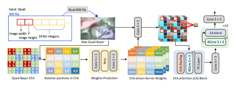
Figure 4: Details of the proposed CFA attention based Quad Bayer remosaicing module (QB-Re block).

4.2 Quad Bayer Remosaicing Block

The neighboring $2\times 2$ cells of the raw Quad Bayer pattern always pertain to distinct channels, whereas the individual pixels within each cell are predominantly representative of a single color, as illustrated in Fig. 2. Consequently, applying convolution on the raw Quad Bayer data directly would lead to distorted spatial information and a loss of channel correlation. To address this issue, this subsection proposes a solution by introducing a Quad Bayer color filter array (CFA)-driven convolution block.

Specifically, the arrangement of a Quad Bayer CFA pattern is a repeating $4\times 4$ grid matrix containing 4 color sensitive sensor cells over the entire grid. To reconstruct a full-resolution Bayer image from such a Quad mosaic, we designe a CFA-aware weight sharing strategy based on CFA layout and its global periodical pattern, which allows the convolution kernel to change its weight periodically when sliding, so that the color distribution in the perceptual field changes periodically. As shown in Fig. 4, for an input Quad Bayer image $\mathbf{I}\in\mathbb{R}^{M\times N}$, its relative positions within the CFA is firstly calculated, then the $\ell$-th channel of feature map $\mathbf{F}_{1}$ is extracted by using the CFA-driven convolution kernel, in which the weights is changed periodically according to $4\times 4$ Quad Bayer pattern,

$$\mathbf{F}_{1}^{\ell}=\sum_{t}\mathbf{K}_{t}^{\ell}*\mathbf{I}_{t},$$ (4)

$$\mathbf{F}_{1}^{\ell}[i,j]=\sum_{p,q}\mathbf{I}_{t}[i+p,j+q]\mathbf{K}_{t}^{\ell}[M-1-p,N-1-q],$$

where * denotes 2D convolution operation, $\mathbf{K}_{t}^{\ell}$ is kernel matrix of shape $M\times N$, which parameterizes a filter according to the relative positions of input image within Quad Bayer CFA. It is designed to ensure that neighboring pixels with the same color have similar spectral distributions, by assigning the same weights to pixels with the same relative positions, i.e.,

$$\mathbf{K}_{t}^{\ell}[i^{\prime},j^{\prime}]=\operatorname{WP}\left((i^{\prime},j^{\prime});\theta\right),$$ (5)

where $\left(i^{\prime},j^{\prime}\right)=(i\bmod 4,j\bmod 4)$ is the relative position of this pixel in the Quad Bayer CFA, $\operatorname{WP}$ is the weight prediction block that predicts the kernel weights by using $\left(i^{\prime},j^{\prime}\right)$. Then, feature $\mathbf{F}_{1}$ is processed by a CFA attention (CA) block, which consists of a CFA pooling layer, two $3\times 3$ residual convolution (RConv) and a fully-connected layer. Specifically, for $\mathbf{F}_{1}\in\mathbb{R}^{M\times N\times C}$, CFA pooling aggregates the feature points with the same relative position,

$$\mathbf{F}_{2}\left(i,j,k)\right)=c\sum_{s=0}^{\frac{M}{4}-1}\sum_{t=0}^{\frac{N}{4}-1}\mathbf{F}_{1}[i+4s,j+4t,k],$$ (6)

where $c=\frac{1}{M/4\times N/4}$. Then, two $3\times 3$ RConv are used to extract attention map $\mathbf{F}_{A}$,

$$\mathbf{F}_{A}=\operatorname{RConv}(\operatorname{RConv}(\mathbf{F}_{2})),$$ (7)

and then $\mathbf{F}_{A}$ is refined by the fully-connected layer. Subsequently, the attention map $\mathbf{F}_{A}$ further passes through a $\operatorname{Conv}3\times 3$ layer. Finally, we stack CA blocks together with two residual convolution layers 10 times, and the output of QB-Re block is generated by using a $\operatorname{Conv}3\times 3$ layer.

Distinguished from CNNs that share the global weights, the proposed QB-Re block allocates different weights to channels with varied colors, by using a CFA-aware weight. To further reduce spatial information loss, a CFA attention module (CA) is also proposed, in which we employ a CFA-sensitive mechanism to aggregate the features, called CFA pooling. It aggregates the features within the same relative position in the CFA, which enables the CA to focus on loading of CFA patterns within each channel.

4.3 Dual-head Joint Remosaic and Denoise

In this subsection, we improve the practicality of remosaicing model for real images that are degraded by mixed noise, by integrating a denoising block into the network through a plug-and-play structure, i.e., remosaicing-denoising. This integration makes the network flexible as denoising modules can be independently improved through pre-training or network design.

Subsequently, we evaluated the advantages and disadvantages of solving the denoising and remosaicing (DN&RM) problem in both the DN&RM and RM&DN orders. In the RM&DN order, the noise loses its independent identically distributed (i.i.d.) property, becoming more complex after the raw image is processed by the remosaic module. Consequently, denoising modules that rely on the i.i.d. assumptions become less effective. On the other hand, the DN&RM order does not involve handling a raw image with complicated noise, making denoising easier to implement. However, some details may be lost in the denoised image due to the absence of a perfect denoising algorithm, which may be amplified by subsequent remosaicing.

To address this issue, we propose a parallel solution with dual-head by integrating both DN&RM and RM&DN strategies together, thus avoiding the issue of determining which step should be performed first. However, the inputs passed into the denoising modules in the two schemes are quite different: one of them is the remosaiced Bayer image with noise, and the other one is the noisy Quad Bayer image. To address this, we customize two specific denoising blocks for each scheme, as depicted in Fig. 3.

Specifically, for the first branch, the input is the noisy Quad Bayer mosaic. As adjacent $2\times 2$ pixels in the Quad sensor often come from the same channel in $R,G$, and $B$, the pixels in adjacent $2\times 2$ squares often have different colors. Therefore, using CNNs that represent as much local information as possible may not be sufficient for effective denoising. Here, we consider both local and non-local information by employing a swin-transformer integrated residual convolution (SC) block [39], and stack it in a multiscale UNet style. This approach incorporates the local modeling capability of the residual convolution and the non-local modeling capability of the swin transformer, resulting in effective denoising of the Quad Bayer mosaic,

$$\left\{\begin{aligned} &\mathbf{Y}_{0}=\operatorname{Conv}3\times 3(\mathbf{O})\in\mathbb{R}^{M\times N\times C}\\ &\mathbf{Y}_{l}=\operatorname{DownS}(\operatorname{SC}(\mathbf{Y}_{0}))\in\mathbb{R}^{\frac{M}{8}\times\frac{N}{8}\times 8C}\\ &\mathbf{Y}_{l+1}=\operatorname{SC}(\mathbf{Y}_{l})\in\mathbb{R}^{\frac{M}{8}\times\frac{N}{8}\times 8C}\\ &\mathbf{Y}_{l+2}=\operatorname{UpS}(\operatorname{SC}(\mathbf{Y}_{l+1}))\in\mathbb{R}^{M\times N\times C}\\ &\mathbf{Y}_{l+3}=\operatorname{Conv}3\times 3(\mathbf{Y}_{l+2})\in\mathbb{R}^{M\times N}\\ &\mathbf{Y}_{l+4}=\operatorname{QB-Re}(\mathbf{Y}_{l+3},\mathbf{Q})\in\mathbb{R}^{M\times N}\end{aligned}\right.$$ (8)

where $\operatorname{DownS,UpS}$ are the down-sampling ($2\times 2$ strided convolution with stride 2) and up-sampling ($2\times 2$ transposed convolution with stride 2), respectively.

For the second branch, the input of DN is the Bayer image processed by QB-Re block, it has small CFA pattern, the $2\times 2$ cell includes pixels from $R,G$ and $B$ channels, and adjacent pixels often belong to different channels, instead of one color for one cell in the Quad image. To effectively increase the perceptual field of view of pixels belonging to different colors, avoiding be entrapped into local CFA patterns, while taking into account the computational power of mobile devices such as mobile phones, we employ DWT-IWT blocks,

$$\left\{\begin{aligned} &\mathbf{X}_{l}=\operatorname{QB-Re}(\mathbf{O},\mathbf{Q})\in\mathbb{R}^{M\times N}\\ &\mathbf{X}_{l+1}=\operatorname{DWT}(\mathbf{X}_{l})\in\mathbb{R}^{\frac{M}{8}\times\frac{N}{8}\times 8C}\\ &\mathbf{X}_{l+2}=\operatorname{PReLu}(\operatorname{Conv}(\mathbf{X}_{l+1}))\in\mathbb{R}^{\frac{M}{8}\times\frac{N}{8}\times 8C}\\ &\mathbf{X}_{l+2}=\operatorname{RG}(\operatorname{RG}(\mathbf{X}_{l+1}))\in\mathbb{R}^{\frac{M}{8}\times\frac{N}{8}\times 8C}\\ &\mathbf{X}_{l+3}=\operatorname{IWT}(\mathbf{X}_{l+2})\in\mathbb{R}^{M\times N}\\ &\mathbf{X}_{l+4}=\operatorname{PReLu}(\operatorname{Conv}(\mathbf{X}_{l+3}))\in\mathbb{R}^{M\times N}\\ \end{aligned}\right.$$ (9)

Moreover, DWT can capture both frequency and location information of feature maps [5, 4], which is also helpful to reduce information loss during denoising phase and feed the subsequent QB-Re block with more information. Subsequently, $\hat{\mathbf{I}}$ is obtained by aggregating $\mathbf{X}_{l+4}$ and $\mathbf{Y}_{l+4}$.

GT W/O fine-tuning W/ fine-tuning GT W/O fine-tuning W/ fine-tuning

Figure 5: After training the proposed DJRD on a standard image dataset, we observed noticeable artifacts such as zippering on thin building windows and Moiré patterns in the fan example. However, fine-tuning the network on challenging cases significantly reduced these artifacts, as seen in the second column.

4.4 Bottleneck Data Mining

On the most general test datasets, most of existing CNN methods can recover images that are visually close to the ground truth. However, when we zoom in locally, a closer inspection reveals artifacts near fine edges and complex textures (see Fig. 5). This suggests that a large number of training samples does not guarantee convincing re-mosaicing. This is mainly caused by the distributional properties of training data. Specifically, the randomly selected images are mainly composed of smooth blocks, as these blocks dominate the natural images [18, 11]. Therefore, with such a training dataset challenging structures account for only a small fraction, smoothed patches occupy the vast majority of the training data, when its number reaches a certain value, the performance improvement brought by continuing to add such training samples is tiny.

To overcome the bottleneck problem, we rebuild a Bottleneck dataset. This dataset comprises 2000 $128\times 128$ hard patches, which include paired Quad Bayer, Bayer, and RGB images. The dataset creation process begins by utilizing our DJRD model, trained on the MIPI dataset, to acquire Bayer images. We then convert these images to the RGB domain using the demosaicing method MIT [11]. Subsequently, we select a database that contains images degraded by two specific artifacts, namely zipper and color Moiré, as illustrated in the second column of Fig. 5. Specifically, we employ the HDR-VDP2 visual metric [11, 26] to identify hard cases featuring zipper artifacts along thin edges. Then, for the Moiré (as the distracting false color bands shown in the fan of Fig. 5), it is caused by the misaliasing of adjacent pixels belonging to different color channels and introduces undesirable low frequency textures. Therefore, we measure the frequencies by quantifying the difference of each frequency as follows:

$$\rho(\omega)=\begin{cases}\log\left(\frac{\left|\mathcal{F}_{\mathrm{CI}}(\omega)\right|^{2}+\eta}{\left|\mathcal{F}_{\mathrm{GT}}(\omega)\right|^{2}+\eta}\right)&\text{ if }|\omega|\leq c\\ 1&\text{ otherwise }\end{cases}$$ (10)

where $\mathcal{F}_{\mathrm{CI}}(\omega)$ and $\mathcal{F}_{\mathrm{GT}}(\omega)$ denote the 2D Fourier transform of each channel of the compared image (CI) and ground truth (GT), respectively. $c=0.95\pi$ is a constant.

With the Bottleneck dataset, the loss function is then effectively reweighed toward difficult patches, by focusing on fitting the hard images while rejecting trivial cases. Fig. 5 illustrates an example of training our network on hard cases, which shows that the reweighed network yielded drastically improved results, especially the zipper and Moiré artifacts.

5 Experiments

5.1 Datasets and Implementation Detail

To better test the performance of the proposed model, we use 210 images with size of $1200\times 1800$, from the latest 2022 MIPI challenge [36], as the basic training set. The training images for all the tested models have three noise levels: 0dB, 24dB and 42dB, all the noise consists of read noise and shot noise. Additionally, the selected hard cases is used to fine-tune the trained model. For equal comparison, in testing, we also use the standard test datasets released by the challenge, which contains 30 images with size of $1200\times 1800$. In addition, two public image datasets: Urban100 [13] and MIT Moiré [11] are chosen as test images. MIT Moiré images consist of 210 images, and the whole Urban100 has 100 high-resolution images.

5.2 Results in Bayer and sRGB Domain

Firstly, it should be noted that there is currently no publicly available full-resolution remosaicing model. Therefore, we evaluate the proposed remosaic model DJRD on the Bayer domain separately. We use the probability distribution difference based Kullback-Leibler divergence (KLD), Peak Signal-to-Noise Ratio (PSNR), and Learned Perceptual Image Patch Similarity (LPIPS) [41]. Tab. 1 shows that our model produces high-quality Bayer images, with a PSNR of over 40 dB and a KLD smaller than 0.025.

Table 1: Quantitative evaluation in Bayer domain, sRGB domain.

Dataset	Metric	Bayer Domain			sRGB
8
		0dB	24dB	42dB	0dB	24dB	42dB
MIPI	KLD	0.0037	0.0096	0.0237	-	-	-
	PSNR	51.51	45.31	40.45	40.58	36.19	32.43
	LPIPS	0.0034	0.0579	0.1366	0.0301	0.1316	0.2305

Subsequently, the proposed model was compared to state-of-the-art Quad Bayer demosaicing methods in the sRGB domain, including the classical joint demosaicing and denoising model [11] (referred to as MIT), the latest deep attention-based PIPNet [1], and SAGAN, which employs adversarial spatial-asymmetric attention [30]. To enable the comparison in the sRGB domain, we used the pre-trained MIT [11] to convert our Bayer images generated by DJRD to sRGB images. Quantitative Results: The proposed model was evaluated using three image quality metrics: PSNR, SSIM, and LPIPS. Tab. 2, 3 present the reconstructed results of all the test modes on images with three noise levels. The results show that our DJRD produces the best overall performance. Specifically, DJRD outperforms PIPNet and SAGAN with 5.68dB and 4.54dB PSNR, respectively. Additionally, there is a 0.04 SSIM gap between DJRD and SAGAN.

Table 2: Quantitative comparison with respect to PSNR, SSIM and LPIPS in sRGB domain on MIT Moiré and Urban100.

Datasets	Method	PSNR $\uparrow$	SSIM $\uparrow$	LPIPS $\downarrow$
Urban100 [13]	MIT [11]	24.87	0.90	0.1217
	PIPNet [1]	26.67	0.93	0.0951
	SAGAN [30]	26.34	0.92	0.1067
	DJRD(Our)	31.02	0.98	0.0348
MIT Moiré [11]	MIT [11]	25.20	0.81	0.1857
	PIPNet [1]	26.04	0.88	0.1740
	SAGAN [30]	26.42	0.87	0.2034
	DJRD(Our)	29.74	0.95	0.0815

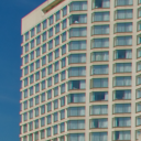
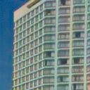
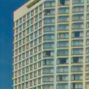
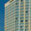
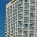
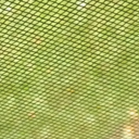
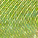
(a) GT

(b) MIT

(c) PIPNet

(d) SAGAN

(e) DJRD

Figure 6: Visual comparison on MIT Moiré and Urban100.

Visual Evaluation: The visual results are shown in Fig. 6, 7, 8. For all the test models, the PSNR of its reconstructed images are over or near 30dB, which means that it is hard to observe obvious differences in a coarse scale. Therefore, to highlight the difference, we enlarge the challenging patches with rich details. From the figures, one can see that most models suffer from residual noise or blurring artifacts. Specifically, Fig. 7 provides the visual results on MIPI dataset with noise level 42dB. In this case the gap between the proposed mode and other methods is obvious, for example, one can observe that both PIPNet and SAGAN fail to recover the net structure, also introducing some distortion in the joints. In contrast, the proposed mode recovers fine structures and preserves the texture in the joints. Fig. 6, 8 show the results on Urban100 and MIT Moiré datasets, one can see that the wall, net and texts reconstructed by our mode preserves more details than PIPNet and SAGAN, which introduce some smoothness. More detailed analysis and discussion please refer to the supplementary material.

Table 3: Quantitative comparison with respect to PSNR, SSIM and LPIPS on test image dataset MIPI.

Noise Level		0dB			24dB			42dB			Average
Dataset	Method	PSNR $\uparrow$	SSIM $\uparrow$	LPIPS $\downarrow$	PSNR $\uparrow$	SSIM $\uparrow$	LPIPS $\downarrow$	PSNR $\uparrow$	SSIM $\uparrow$	LPIPS $\downarrow$	PSNR $\uparrow$	SSIM $\uparrow$	LPIPS $\downarrow$
MIPI [36]	MIT [11]	30.39	0.89	0.1437	29.92	0.87	0.2024	27.93	0.79	0.3501	29.41	0.85	0.2321
	PIPNet [1]	32.32	0.95	0.1252	31.26	0.92	0.1800	28.44	0.87	0.2928	30.67	0.91	0.1993
	SAGAN [30]	33.36	0.95	0.1161	32.40	0.92	0.1705	29.66	0.87	0.2714	31.81	0.91	0.1860
	DJRD(Ours)	40.58	0.97	0.0301	36.19	0.93	0.1316	32.43	0.89	0.2305	36.40	0.93	0.1307

MIPI-Quad-071: Quad Bayer Mosaic Input: Noisy Quad Bayer Bayer by DJRD (Our) MIT [11] PIPNet [1] KLD = 0.009 (28.52, 0.80) (28.66, 0.82) Ground Truth in Bayer Domain Ground Truth in RGB Domain SAGAN [30] Our (DJRD+MIT) (PSNR, SSIM) (29.85, 0.85) (31.93, 0.90)

MIPI-Quad-082: Quad Bayer Mosaic Input: Noisy Quad Bayer Bayer by DJRD(Our) MIT [11] PIPNet [1] KLD = 0.012 (30.37, 0.81) (30.41, 0.81) Ground Truth in Bayer Domain Ground Truth in RGB Domain SAGAN [30] Our (DJRD+MIT) (PSNR, SSIM) (31.87, 0.85) (34.05, 0.90)

Figure 7: Visual comparison of Quad Bayer joint remosaicing and denoising methods om MIPI dataset.

Urban100-007 in RGB Domain Ground Truth in RGB Domain MIT [11] SAGAN [30] Our (DJRD+MIT) Ground Truth in RGB Domain MIT [11] SAGAN [30] Our (DJRD+MIT)

Figure 8: Visual comparison of Quad Bayer joint remosaicing and denoising methods on Urban100 dataset.

5.3 Ablation Studies

To verify the effectiveness of the employed or designed sub-modules, we decomposed the entire model into degraded models containing only a subset of components and trained them independently. Tab. 4 presents the PSNR and SSIM values obtained by evaluating the different modules of the proposed network. The results demonstrate that our proposed components significantly enhance the quality of reconstructed images, even in the presence of different levels of noise degradation. More details and discussions are available in the supplementary material.

Table 4: Ablation studies on six distinct configurations of our method on MIPI, DN-RM: denoise first then remosaic, DN-RM+hard: fine tune the network with hard cases, Dual+Hard: using the dual-head pipeline fine-tuning on hard cases.

Noise Level	0 dB		24 dB		42 dB		Average
Tactics	PSNR	SSIM	PSNR	SSIM	PSNR	SSIM	PSNR	SSIM
DN-RM	38.35	0.9576	35.51	0.9146	31.91	0.8589	35.26	0.9104
RM-DN	39.21	0.9587	35.57	0.9145	32.01	0.8590	35.59	0.9107
DN-RM+Hard	39.95	0.9635	35.90	0.9170	31.98	0.8594	35.94	0.9133
RM-DN+Hard	40.15	0.9652	35.86	0.9164	32.16	0.8612	36.06	0.9143
Dual+Hard	40.58	0.9662	36.19	0.9192	32.43	0.8659	36.40	0.9171

6 Conclusion

In this paper, we have presented a dual-head joint remosaicing and denoising network that is capable of converting noisy Quad Bayer and clean classical Bayer mosaic of low-light imaging cameras without any resolution loss. Our approach not only facilitates the use of all software and hardware designed for classic Bayer CFA but also allows for any advances in Bayer CFA tools to be directly applicable to Quad sensor. Furthermore, our model outperforms the SOTA, yielding a 3dB performance boost under practical noise degradation, which demonstrates the potential of our approach in improving low-light image quality.

References

- [1] SM A Sharif, Rizwan Ali Naqvi, and Mithun Biswas. Beyond joint demosaicking and denoising: An image processing pipeline for a pixel-bin image sensor. In Proceedings of the IEEE/CVF Conference on Computer Vision and Pattern Recognition, pages 233–242, 2021.
- [2] Tawsin Uddin Ahmed, Seyed Ali Amirshahi, and Marius Pedersen. Image demosaicing: Subjective analysis and evaluation of image quality metrics. Image, 30:25, 2023.
- [3] David Alleysson, Sabine Susstrunk, and Jeanny Hérault. Linear demosaicing inspired by the human visual system. IEEE Transactions on Image Processing, 14(4):439–449, 2005.
- [4] Ingrid Daubechies. The wavelet transform, time-frequency localization and signal analysis. IEEE transactions on information theory, 36(5):961–1005, 1990.
- [5] Ingrid Daubechies. Ten lectures on wavelets. SIAM, 1992.
- [6] Valéry Dewil, Adrien Courtois, Mariano Rodríguez, Thibaud Ehret, Nicola Brandonisio, Denis Bujoreanu, Gabriele Facciolo, and Pablo Arias. Video joint denoising and demosaicing with recurrent cnns. In Proceedings of the IEEE/CVF Winter Conference on Applications of Computer Vision, pages 5108–5119, 2023.
- [7] Xingbo Dong, Wanyan Xu, Zhihui Miao, Lan Ma, Chao Zhang, Jiewen Yang, Zhe Jin, Andrew Beng Jin Teoh, and Jiajun Shen. Abandoning the bayer-filter to see in the dark. In Proceedings of the IEEE/CVF Conference on Computer Vision and Pattern Recognition, pages 17431–17440, 2022.
- [8] Eric Dubois. Frequency-domain methods for demosaicking of bayer-sampled color images. IEEE Signal Processing Letters, 12(12):847–850, 2005.
- [9] Thibaud Ehret, Axel Davy, Pablo Arias, and Gabriele Facciolo. Joint demosaicking and denoising by fine-tuning of bursts of raw images. In Proceedings of the IEEE/CVF International Conference on Computer Vision, pages 8868–8877, 2019.
- [10] Kai Feng, Yongqiang Zhao, Jonathan Cheung-Wai Chan, Seong G Kong, Xun Zhang, and Binglu Wang. Mosaic convolution-attention network for demosaicing multispectral filter array images. IEEE Transactions on Computational Imaging, 7:864–878, 2021.
- [11] Michaël Gharbi, Gaurav Chaurasia, Sylvain Paris, and Frédo Durand. Deep joint demosaicking and denoising. ACM Transactions on Graphics (ToG), 35(6):1–12, 2016.
- [12] Shi Guo, Zhetong Liang, and Lei Zhang. Joint denoising and demosaicking with green channel prior for real-world burst images. IEEE Transactions on Image Processing, 30:6930–6942, 2021.
- [13] Jia-Bin Huang, Abhishek Singh, and Narendra Ahuja. Single image super-resolution from transformed self-exemplars. In Proceedings of the IEEE conference on computer vision and pattern recognition, pages 5197–5206, 2015.
- [14] Andrey Ignatov, Nikolay Kobyshev, Radu Timofte, Kenneth Vanhoey, and Luc Van Gool. Dslr-quality photos on mobile devices with deep convolutional networks. In Proceedings of the IEEE International Conference on Computer Vision, pages 3277–3285, 2017.
- [15] Irina Kim, Dongpan Lim, Youngil Seo, Jeongguk Lee, Yunseok Choi, and Seongwook Song. On recent results in demosaicing of samsung 108mp cmos sensor using deep learning. In 2021 IEEE Region 10 Symposium (TENSYMP), pages 1–4. IEEE, 2021.
- [16] Irina Kim, Seongwook Song, Soonkeun Chang, Sukhwan Lim, and Kai Guo. Deep image demosaicing for submicron image sensors. Electronic Imaging, 2020(7):60410–1, 2020.
- [17] Yongnam Kim and Yunkyung Kim. High-sensitivity pixels with a quad-wrgb color filter and spatial deep-trench isolation. Sensors, 19(21):4653, 2019.
- [18] Anat Levin, Boaz Nadler, Fredo Durand, and William T Freeman. Patch complexity, finite pixel correlations and optimal denoising. In European Conference on Computer Vision, pages 73–86. Springer, 2012.
- [19] Yijun Li, Jia-Bin Huang, Narendra Ahuja, and Ming-Hsuan Yang. Deep joint image filtering. In European conference on computer vision, pages 154–169. Springer, 2016.
- [20] Jiaming Liu, Chi-Hao Wu, Yuzhi Wang, Qin Xu, Yuqian Zhou, Haibin Huang, Chuan Wang, Shaofan Cai, Yifan Ding, Haoqiang Fan, et al. Learning raw image denoising with bayer pattern unification and bayer preserving augmentation. In Proceedings of the IEEE/CVF Conference on Computer Vision and Pattern Recognition Workshops, pages 0–0, 2019.
- [21] Lin Liu, Xu Jia, Jianzhuang Liu, and Qi Tian. Joint demosaicing and denoising with self guidance. In Proceedings of the IEEE/CVF Conference on Computer Vision and Pattern Recognition, pages 2240–2249, 2020.
- [22] Pengju Liu, Hongzhi Zhang, Kai Zhang, Liang Lin, and Wangmeng Zuo. Multi-level wavelet-cnn for image restoration. In Proceedings of the IEEE conference on computer vision and pattern recognition workshops, pages 773–782, 2018.
- [23] Ze Liu, Yutong Lin, Yue Cao, Han Hu, Yixuan Wei, Zheng Zhang, Stephen Lin, and Baining Guo. Swin transformer: Hierarchical vision transformer using shifted windows. In Proceedings of the IEEE/CVF international conference on computer vision, pages 10012–10022, 2021.
- [24] Karima Ma, Michael Gharbi, Andrew Adams, Shoaib Kamil, Tzu-Mao Li, Connelly Barnes, and Jonathan Ragan-Kelley. Searching for fast demosaicking algorithms. ACM Transactions on Graphics (TOG), 41(5):1–18, 2022.
- [25] Henrique S Malvar, Li-wei He, and Ross Cutler. High-quality linear interpolation for demosaicing of bayer-patterned color images. In 2004 IEEE International Conference on Acoustics, Speech, and Signal Processing, volume 3, pages iii–485. IEEE, 2004.
- [26] Rafał Mantiuk, Kil Joong Kim, Allan G Rempel, and Wolfgang Heidrich. Hdr-vdp-2: A calibrated visual metric for visibility and quality predictions in all luminance conditions. ACM Transactions on graphics (TOG), 30(4):1–14, 2011.
- [27] Kangfu Mei, Juncheng Li, Jiajie Zhang, Haoyu Wu, Jie Li, and Rui Huang. Higher-resolution network for image demosaicing and enhancing. In 2019 IEEE/CVF International Conference on Computer Vision Workshop (ICCVW), pages 3441–3448. IEEE, 2019.
- [28] Jayanta Mukherjee, R Parthasarathi, and Sachin Goyal. Markov random field processing for color demosaicing. Pattern Recognition Letters, 22(3-4):339–351, 2001.
- [29] Olaf Ronneberger, Philipp Fischer, and Thomas Brox. U-net: Convolutional networks for biomedical image segmentation. In International Conference on Medical image computing and computer-assisted intervention, pages 234–241. Springer, 2015.
- [30] SMA Sharif, Rizwan Ali Naqvi, and Mithun Biswas. Sagan: Adversarial spatial-asymmetric attention for noisy nona-bayer reconstruction. arXiv preprint arXiv:2110.08619, 2021.
- [31] Ana Stojkovic, Ivana Shopovska, Hiep Luong, Jan Aelterman, Ljubomir Jovanov, and Wilfried Philips. The effect of the color filter array layout choice on state-of-the-art demosaicing. Sensors, 19(14):3215, 2019.
- [32] Daniel Stanley Tan, Wei-Yang Chen, and Kai-Lung Hua. Deepdemosaicking: Adaptive image demosaicking via multiple deep fully convolutional networks. IEEE Transactions on Image Processing, 27(5):2408–2419, 2018.
- [33] Runjie Tan, Kai Zhang, Wangmeng Zuo, and Lei Zhang. Color image demosaicking via deep residual learning. In Proc. IEEE Int. Conf. Multimedia Expo (ICME), pages 793–798, 2017.
- [34] Chi-Yi Tsai and Kai-Tai Song. A new edge-adaptive demosaicing algorithm for color filter arrays. Image and Vision Computing, 25(9):1495–1508, 2007.
- [35] Wenzhu Xing and Karen Egiazarian. End-to-end learning for joint image demosaicing, denoising and super-resolution. In Proceedings of the IEEE/CVF Conference on Computer Vision and Pattern Recognition, pages 3507–3516, 2021.
- [36] Qingyu Yang, Guang Yang, Jun Jiang, Chongyi Li, Ruicheng Feng, Shangchen Zhou, Wenxiu Sun, Qingpeng Zhu, Chen Change Loy, and Jinwei Gu. Mipi 2022 challenge on quad-bayer re-mosaic: Dataset and report. arXiv preprint arXiv:2209.07060, 2022.
- [37] Yoonjong Yoo, Jaehyun Im, and Joonki Paik. Low-light image enhancement using adaptive digital pixel binning. Sensors, 15(7):14917–14931, 2015.
- [38] Chao Zhang, Yan Li, Jue Wang, and Pengwei Hao. Universal demosaicking of color filter arrays. IEEE Transactions on Image Processing, 25(11):5173–5186, 2016.
- [39] Kai Zhang, Yawei Li, Jingyun Liang, Jiezhang Cao, Yulun Zhang, Hao Tang, Radu Timofte, and Luc Van Gool. Practical blind denoising via swin-conv-unet and data synthesis. arXiv preprint arXiv:2203.13278, 2022.
- [40] Lei Zhang and Xiaolin Wu. Color demosaicking via directional linear minimum mean square-error estimation. IEEE Transactions on Image Processing, 14(12):2167–2178, 2005.
- [41] Richard Zhang, Phillip Isola, Alexei A Efros, Eli Shechtman, and Oliver Wang. The unreasonable effectiveness of deep features as a perceptual metric. In Proceedings of the IEEE conference on computer vision and pattern recognition, pages 586–595, 2018.
- [42] Tao Zhang, Ying Fu, and Cheng Li. Deep spatial adaptive network for real image demosaicing. In Proceedings of the AAAI Conference on Artificial Intelligence, volume 36, pages 3326–3334, 2022.