Confidence Intervals for Ratios of Proportions in Stratified Bilateral Correlated Data

Abstract

Confidence interval (CI) methods for stratified bilateral studies use intraclass correlation to avoid misleading results. In this article, we propose four CI methods (sample-size weighted global MLE-based Wald-type CI, complete MLE-based Wald-type CI, profile likelihood CI, and complete MLE-based score CI) to investigate CIs of proportion ratios to clinical trial design with stratified bilateral data under Dallal’s intraclass model. Monte Carlo simulations are performed, and the complete MLE-based score confidence interval (CS) method yields a robust outcome. Lastly, a real data example is conducted to illustrate the proposed four CIs.

1 Introduction

In random clinical trials, we often encounter bilateral data in patients who receive the treatment based on paired body parts or organs (such as eyes, ears, kidneys, etc.). Although different studies from different aspects constructed statistical significance tests for bilateral data, the confidence interval (CI) construction becomes a trend, which provides more information than statistical significance tests. Several studies developed CIs for proportion ratio in two independent binomial proportions, such as Gart and Nam and Koopman [1, 2]. Still, none of those studies take the intraclass correlation into consideration when dealing with bilateral data.

Ignoring correlations in the correlated data leads to error, which has been found in Sainani’s study [3]. To address this problem, Rosner proposed that a conditional probability of response at one side of paired body parts or organs gives a response at the other body parts or organs is a positive constant R time the response rate [4]. Related to this, Donner assumed that all treatment groups share one intraclass correlation coefficient $\rho$ [5]. Following this stream of literature, several studies have proposed constructing CIs under these two models with considerable progress. Under Rosner’s R model, Peng et al. developed asymptotic CIs of proportion ratios in correlated paired data [6]. Tang et al. proposed CIs construction of the difference between two correlated proportions with missing observations [7]. Tang et al. presented a confidence interval approach for comparative studies involving binary outcomes in paired organs [8]. Yang et al. constructed the CIs for many-to-one comparisons of proportion differences in correlated paired data [9]. Wang and Shan considered the relative risk and the odds ratio of exact CIs [10]. Under Donnar’s model, Li and Ma constructed asymptotic tests and CIs for the odds ratio of two proportions in bilateral correlated data[11]. Pei et al. presented the CIs for correlated proportion differences from paired data in a two-arm randomized clinical trial [12].

However, Dallal criticizes Rosner’s assumption and points out that “the constant R model will give a poor fit if the characteristic is almost certain to occur bilaterally with widely varying group-specific prevalence” [13]. Dallal believes the conditional probability of response at one side of paired body parts or organs, giving a response at the other body parts or organs is a constant $\gamma$ [13].

Under the stratified bilateral correlated data framework, several studies have developed various CIs with different intraclass models. Xue and Ma developed CIs for proportion ratios using Rosner’s R model [14]. Zhuang et al. constructed CIs for proportion ratios with Donner’s $\rho$ model [15]. Shen et al. presented CIs for risk difference with Donner’s $\rho$ model [16]. Tang et al. introduced CIs for risk differences in stratified paired designs under Rosner’s R model [17]. However, constructing CIs under Dallal’s intraclass model in stratified bilateral correlated data has not been explored yet, especially the CIs for proportion ratio. The primary goal of this article is to investigate CIs of proportion ratios to clinical trial design with stratified bilateral data under Dallal’s intraclass model.

The remainder of this paper is organized as follows: section 2 presents the data structure and hypotheses, and section 3 introduces the maximum-likelihood estimation under each hypothesis. We propose four confidence interval construction methods for proportion ratio under Dallal’s model in section 4. Accordingly, we investigate the performance and robustness of four confidence interval construction methods by using simulation studies in section 5. Section 6 uses a real example of the OME study to illustrate our proposed methods. Conclusions and future works are in section 7.

2 Data structure and Hypotheses

2.1 Notation

Let $m_{lij}$ be the number of patients in the $i^{th}$ group of the $j^{th}$ stratum with $l^{th}$ responses, where $i$ = 1,2, $j=1,\ldots,J$ , $l$ = 0, 1, 2. $m_{+ij}=m_{0ij}+m_{1ij}+m_{2ij}$ represent the number of patients in the $i^{th}$ group of the $j^{th}$ stratum. The $p_{lij}$ is corresponding to the probability of patients in $i^{th}$ group of the $j^{th}$ stratum with $l^{th}$ responses. Define $Z_{ijkh}$ as the indicator of the response of $k^{th}$ eyes of the $h^{th}$ patient in the $i^{th}$ group from $j^{th}$ stratum, where $k$ = 1, 2 and $h=1,2,\ldots,m_{+ij}$. If $Z_{ijkh}=1$ then the improvement response occurs, and $Z_{ijkh}=0$ otherwise. Therefore, donate $\operatorname{Pr}\left(Z_{hijk}=1\right)=\pi_{ij},\left(0\leq\pi_{ij}\leq 1\right)$ as probability of having response on one site.

$$\begin{array}[]{cccc}\hline\cr&\lx@intercol\hfil\text{ Group }\hfil\lx@intercol\\ \cline{2-3}\cr\text{ Number of Responses }(l)&1&2&\quad\text{ Total }\\ \hline\cr 0&m_{01j}\left(p_{01j}\right)&m_{02j}\left(p_{02j}\right)&m_{0+j}\\ 1&m_{11j}\left(p_{11j}\right)&m_{12j}\left(p_{12j}\right)&m_{1+j}\\ 2&m_{21j}\left(p_{21j}\right)&m_{22j}\left(p_{22j}\right)&m_{2+j}\\ \hline\cr\text{ Total }&m_{+1j}&m_{+2j}&m_{++j}\\ \hline\cr\end{array}$$

We explore the intraclass correlation based on Dallal’s model that is conditional probability of response at one side of paired body parts or organs, giving a response at the other body parts or organs is a constant $\gamma$. Therefore, we assume $P\left(Z_{hijk}=1\mid Z_{hij(3-k)}=1\right)=\gamma_{j}$, and the probabilities of eye with none, one or both can be express as following:

$$p_{0ij}=1-\left(2-\gamma_{j}\right)\pi_{ij},$$

$$\quad p_{1ij}=2\pi_{ij}\left(1-\gamma_{j}\right),$$

$$\quad p_{2ij}=\pi_{ij}\gamma_{j},$$

and $p_{0ij}+p_{1ij}+p_{2ij}=1$ for any fixed $i$ and $j$. The joint likelihood function for the observed data $\boldsymbol{m_{ij}}=\left(m_{0ij},m_{1ij},m_{2ij}\right)^{T}$ is given by

$$f\left(\boldsymbol{m_{ij}}\mid\boldsymbol{p_{ij}}\right)=\prod_{j=1}^{J}\prod_{i=1}^{2}\frac{m_{+ij}!}{m_{0ij}!m_{1ij}!m_{2ij}!}p_{0ij}^{m_{0ij}}p_{1ij}^{m_{1ij}}p_{2ij}^{m_{2ij}},$$

where $\boldsymbol{p_{ij}}=\left(p_{0ij},p_{1ij},p_{2ij}\right)^{T}$. The corresponding log-likelihood function can be expressed as:

$$l\left(\boldsymbol{\pi_{i}},\boldsymbol{\gamma}\right)=\sum_{j=1}^{J}\sum_{i=1}^{2}\left\{m_{0ij}\log\left[1-\left(2-\gamma_{j}\right)\pi_{ij}\right]+m_{1ij}\log\left[2\pi_{ij}\left(1-\gamma_{j}\right)\right]+m_{2ij}\log\left[\pi_{ij}\gamma_{j}\right]\right\}+\log C,$$

where $\boldsymbol{\pi_{i}}=\left(\pi_{i1},\ldots,\pi_{iJ}\right)^{T}$, $\boldsymbol{\gamma}=\left(\gamma_{1},\ldots,\gamma_{J}\right)^{T}$, and $C=\prod_{j=1}^{J}\prod_{i=1}^{2}\frac{m_{+ij}!}{m_{0ij}!m_{1ij}!m_{2ij}!}$ is a constant.

2.2 Hypotheses for the proportion ratio across strata

Assuming the ratio of proportions between two groups in the $j^{\text{th }}$ stratum is $\delta_{j}=\pi_{2j}/\pi_{1j}$ for $j=1,\ldots,J$, we construct three hypotheses as follows:

$$H:\delta_{1}=\delta_{2}=...=\delta_{J}\quad\text{(unconstrained hypothesis)},$$

$$H:\delta_{1}=\delta_{2}=...=\delta_{J}=\delta_{0}\quad\text{(constrained hypothesis)},$$

$$H:\delta_{1}\neq\delta_{2}\neq...\neq\delta_{J}\quad\text{(global hypothesis)}.$$

Different hypotheses are based on different research questions: unconstrained hypothesis usually is used to test the homogeneity across strata; the constrained hypothesis indicates the common ratio of proportions by giving a constrained value of $\delta_{0}$; and the global hypothesis shows that none of $\delta$ are equal between strata.

3 Maximum-likelihood estimation (MLE) under each hypothesis

3.1 The unconstrained MLEs

Since we assume $\delta_{j}=\pi_{2j}/\pi_{1j}$ for $j=1,\ldots,J$, then $\pi_{2j}=\delta_{j}\pi_{1j}$, under the null hypothesis with common $\delta$, the log-likelihood ratio can be express as:

$$l\left(\boldsymbol{\pi_{1}},\delta,\boldsymbol{\gamma}\right)=\sum_{j=1}^{J}l_{j}\left(\pi_{1j},\delta,\gamma_{j}\right),$$

where

$$\quad l_{j}\left(\pi_{1j},\delta,\gamma_{j}\right) =\{m_{01j}\log\left[1-\left(2-\gamma_{j}\right)\pi_{1j}\right]+m_{11j}\log\left[2\pi_{1j}\left(1-\gamma_{j}\right)\right]+m_{21j}\log\left[\pi_{1j}\gamma_{j}\right]$$

$$+m_{02j}\log\left[1-\left(2-\gamma_{j}\right)\pi_{1j}\delta\right]+m_{12j}\log\left[2\pi_{1j}\delta\left(1-\gamma_{j}\right)\right]+m_{22j}\log\left[\pi_{1j}\delta\gamma_{j}\right]\}$$

$$+\log C.$$

Differentiating $l\left(\boldsymbol{\pi_{1}},\delta,\boldsymbol{\gamma}\right)$ with respect to $\boldsymbol{\pi_{1}}$ and $\boldsymbol{\gamma}$ , we have

$$\frac{\partial l}{\partial\pi_{1j}}=\frac{m_{1+j}}{\pi_{1j}}+\frac{m_{2+j}}{\pi_{1j}}+\frac{m_{01j}\,\left(\gamma_{j}-2\right)}{\pi_{1j}\,\left(\gamma_{j}-2\right)+1}+\frac{\delta\,m_{02j}\,\left(\gamma_{j}-2\right)}{\delta\,\pi_{1j}\,\left(\gamma_{j}-2\right)+1},$$

$$\frac{\partial l}{\partial\gamma_{j}}=\frac{m_{21j}}{\gamma_{j}}+\frac{m_{22j}}{\gamma_{j}}+\frac{m_{11j}}{\gamma_{j}-1}+\frac{m_{12j}}{\gamma_{j}-1}+\frac{m_{01j}\,\pi_{1j}}{\pi_{1j}\,\left(\gamma_{j}-2\right)+1}+\frac{\delta\,m_{02j}\,\pi_{1j}}{\delta\,\pi_{1j}\,\left(\gamma_{j}-2\right)+1}.$$

We can set $\frac{\partial l}{\partial\pi_{1j}}=0$ with $\frac{\partial l}{\partial\gamma_{j}}=0$ to get MLEs $\hat{\pi}_{1j}$ and $\hat{\gamma}_{j}$. Indeed, MLE of $\gamma_{j}$ has closed-form solution. Meanwhile, MLE of $\pi_{1j}$ is a function of $m$ and $\delta$. For the MLE of $\delta$, we will update by using Fisher scoring iterative algorithm, and

$$\hat{\delta}=\delta^{(t+1)}=\delta^{(t)}+\left.I^{-1}\left(\delta^{(t)}\right)\left(\frac{\partial l}{\partial\delta}\right)\right|_{\delta=\delta(t),\hat{\pi}_{1j},\hat{\gamma_{j}}},$$

where

$$\frac{\partial l}{\partial\delta}=\sum_{j=1}^{J}(\frac{m_{12j}}{\delta}+\frac{m_{22j}}{\delta}+\frac{m_{02j}\,\pi_{1j}\,{\left(\gamma_{j}-2\right)}}{\delta\,\pi_{1j}\,{\left(\gamma_{j}-2\right)}+1}),$$

$$\frac{\partial^{2}l}{\partial\delta^{2}}=\sum_{j=1}^{J}(-\frac{m_{12j}}{\delta^{2}}-\frac{m_{22j}}{\delta^{2}}-\frac{m_{02j}\,{\pi_{1j}}^{2}\,{{\left(\gamma_{j}-2\right)}}^{2}}{{{\left(\delta\,\pi_{1j}\,{\left(\gamma_{j}-2\right)}+1\right)}}^{2}}),$$

and

$$I=-E(\frac{\partial^{2}l}{\partial\delta^{2}}) =-E(\sum_{j=1}^{J}(-\frac{m_{12j}}{\delta^{2}}-\frac{m_{22j}}{\delta^{2}}-\frac{m_{02j}\,{\pi_{1j}}^{2}\,{{\left(\gamma_{j}-2\right)}}^{2}}{{{\left(\delta\,\pi_{1j}\,{\left(\gamma_{j}-2\right)}+1\right)}}^{2}}))$$

$$=\sum_{j=1}^{J}(\frac{m_{+2j}p_{12j}}{\delta^{2}}+\frac{m_{+2j}p_{22j}}{\delta^{2}}+\frac{m_{+2j}p_{02j}\,{\pi_{1j}}^{2}\,{{\left(\gamma_{j}-2\right)}}^{2}}{{{\left(\delta\,\pi_{1j}\,{\left(\gamma_{j}-2\right)}+1\right)}}^{2}}).$$

3.2 The constrained MLEs

The constrained hypothesis is nested within the unconstrained hypothesis, and the estimators of unconstrained MLEs are denoted as $\hat{\delta}$, $\hat{\pi}_{1j}$, and $\hat{\gamma_{j}}$. Under the constrained hypothesis, we have $\pi_{2j}=\delta_{0}\pi_{1j}$ for all j. We can directly conclude that the constrained MLEs $\hat{\pi}_{1j_{H_{0}}}$, and $\hat{\gamma_{j}}_{H_{0}}$ have the same function as unconstrained MLEs by replacing $\delta$ with $\delta_{0}$.

3.3 The Global MLEs

Under the global hypothesis, $H_{a}:\delta_{1}\neq\delta_{2}\neq...\neq\delta_{J}$ , the log-likelihood can be presented as:

$$l\left(\boldsymbol{\pi_{1}},\boldsymbol{\delta},\boldsymbol{\gamma}\right)=\sum_{j=1}^{J}l_{j}\left(\pi_{1j},\delta_{j},\gamma_{j}\right),$$

where

$$\quad l_{j}\left(\pi_{1j},\delta_{j},\gamma_{j}\right) =\sum_{j=1}^{J}\left\{m_{01j}\log\left[1-\left(2-\gamma_{j}\right)\pi_{1j}\right]\right.+m_{11j}\log\left[2\pi_{1j}\left(1-\gamma_{j}\right)\right]+m_{21j}\log\left[\pi_{1j}\gamma_{j}\right]$$

$$+m_{02j}\log\left[1-\left(2-\gamma_{j}\right)\pi_{1j}\delta_{j}\right]+m_{12j}\log\left[2\pi_{1j}\delta_{j}\left(1-\gamma_{j}\right)\right]\left.+m_{22j}\log\left[\pi_{1j}\delta_{j}\gamma_{j}\right]\right\}+\log C,$$

and the MLEs of three parameters $\pi_{1j}$, $\delta_{j}$, $\gamma_{j}$ can be derivied by setting the partial differentiation equal to zero, then the MLEs as following:

$$\tilde{\pi}_{1j}=\frac{{\left(m_{11j}+m_{21j}\right)}\,{\left(m_{11j}+m_{12j}+2\,m_{21j}+2\,m_{22j}\right)}}{2\,{\left(m_{01j}+m_{11j}+m_{21j}\right)}\,{\left(m_{11j}+m_{12j}+m_{21j}+m_{22j}\right)}},$$

$$\tilde{\gamma}_{j}=\frac{2\,m_{2+j}}{m_{1+j}+2\,m_{2+j}},$$

$$\tilde{\delta_{j}}=-\frac{{\left(m_{12j}+m_{22j}\right)}\,{\left(m_{01j}-m_{12j}+m_{1+j}-m_{22j}+m_{2+j}\right)}}{{\left(m_{02j}+m_{12j}+m_{22j}\right)}\,{\left(m_{12j}-m_{1+j}+m_{22j}-m_{2+j}\right)}}.$$

4 Confidence interval construction

4.1 Sample-size weighted global MLE-based Wald-type confidence interval (SGW)

The sample-size weighted global MLE-based Wald-type confidence interval (SGW) is widely applied in stratified designs, and the idea of SGW places more weight on the stratum, resulting in more contribution to the overall sample [15, 14]. SGW is constructed by the global hypothesis: $\delta_{1}\neq\delta_{2}\neq...\neq\delta_{J}$, suppose that the MLEs of $\boldsymbol{\beta_{j}}=\left(\delta_{j},\pi_{1j},\gamma_{j}\right)$ be $\boldsymbol{\tilde{\beta}_{j}}=\left(\tilde{\delta}_{j},\tilde{\pi}_{1j},\tilde{\gamma}_{j}\right)$. Under regularity conditions, we have

$$\sqrt{n}\left(\tilde{\boldsymbol{\beta}}_{j}^{T}-\boldsymbol{\beta}_{j}^{T}\right)\stackrel{{\scriptstyle d}}{{\rightarrow}}N_{3}\left(\boldsymbol{0},I_{j}^{-1}\right),$$

where $I_{j}$ is the Fisher information matrix of $\beta_{j}$. Let $c=(1,0,0)$, we can construct MLE of $\delta_{j}$ by $\tilde{\delta_{j}}=c\tilde{\boldsymbol{\beta}}_{j}^{T}$, and the asymptotic distribution of $\tilde{\delta_{j}}$ is:

$$\sqrt{n}\left(\tilde{\delta}_{j}-\delta_{j}\right)\stackrel{{\scriptstyle d}}{{\rightarrow}}N\left(0,cI_{j}^{-1}c^{T}\right).$$

Suppose the overall ratio of proportions is a linear combination of independent within stratum ratios of proportions, then the estimator $\tilde{\delta}=\sum_{j=1}^{\prime}w_{j}\tilde{\delta}_{j}$, where $w_{j}$ ’s are the weights for each stratum and restrict by $\sum_{j=1}^{J}w_{j}\delta_{j}=\delta,\quad\sum_{j=1}^{J}w_{j}=1.$ Therefore, the $100(1-\alpha)\%$ sample-size weighted global MLE-based Wald-type confidence limits of $\delta$ are defined as

$$\sum_{j=1}^{J}w_{j}c\tilde{\boldsymbol{\beta}}_{j}^{T}\mp z_{1-\alpha/2}\sqrt{\sum_{j=1}^{J}w_{j}^{2}cI_{j}^{-1}c^{T}},$$

where $z_{1-\alpha/2}$ is the $100(1-\alpha/2)$ percentile of the standard normal distribution.

By using the sample-size weight method, we assume $w_{j}=\frac{m_{++j}}{N},\quad j=1,\ldots,J$, where $m_{++j}$ indicate the sample size of the $j^{\text{th }}$ stratum and $N$ present as the total sample size. Intuitively, the $100(1-\alpha)\%$ sample size weighted Wald-type confidence limits are

$$\begin{gathered}\mathrm{LCL}_{SGW}=\max\left\{0,\sum_{j=1}^{J}\frac{m_{++j}}{N}c\tilde{\boldsymbol{\beta}}_{j}^{T}-z_{1-\alpha/2}\sqrt{\sum_{j=1}^{J}\left(\frac{m_{++j}}{N}\right)^{2}cI_{j}^{-1}c^{T}}\right\},\\ \mathrm{UCL}_{SGW}=\sum_{j=1}^{J}\frac{m_{++j}}{N}c\tilde{\boldsymbol{\beta}}_{j}^{T}+z_{1-\alpha/2}\sqrt{\sum_{j=1}^{J}\left(\frac{m_{++j}}{N}\right)^{2}cI_{j}^{-1}c^{T}}.\end{gathered}$$

4.2 Complete MLE-based Wald-type confidence interval (CW)

We consider another Wald-type confidence interval method, named complete MLE-based Wald-type confidence interval (CW). This method is under unconstrained hypothesis: $\delta_{1}=\delta_{2}=\cdots=\delta_{J}$, with considering homogeneity of proportion ratios. The MLEs of $\boldsymbol{\beta}=\left(\delta,\boldsymbol{\pi_{1}},\boldsymbol{\gamma}\right)$ be $\hat{\boldsymbol{\beta}}=\left(\hat{\delta},\hat{\boldsymbol{\pi}}_{1},\hat{\boldsymbol{\gamma}}\right)$. Under regularity conditions, we have

$$\sqrt{n}\left(\hat{\boldsymbol{\beta}}^{T}-\boldsymbol{\beta}^{T}\right)\stackrel{{\scriptstyle d}}{{\rightarrow}}N_{1+2J}\left(0,I^{-1}\right),$$

and $I$ corresponding to the fisher information matrix of $\beta$ (See Appendix for details). Assume $C=(1,0,\ldots,0)_{1\times(1+2J)}$, the MLE of $\delta$ can be written as $\hat{\delta}=C\hat{\beta}^{T}$. By applying delta method, the asymptotic distribution of $\hat{\delta}$ is

$$\sqrt{n}(\hat{\delta}-\delta)\stackrel{{\scriptstyle d}}{{\rightarrow}}N\left(0,CI^{-1}C^{T}\right).$$

The $100(1-\alpha)\%$ of complete MLE-based Wald-type confidence limits are defined as

$$\begin{gathered}\mathrm{LCL}_{CW}=\max\left\{0,{C}\hat{\boldsymbol{\beta}}^{T}-z_{1-\alpha/2}\sqrt{\left.{C}{I}^{-1}{C}^{T}\right\}},\right.\\ \mathrm{UCL}_{CW}=C\hat{\boldsymbol{\beta}}^{T}+z_{1-\alpha/2}\sqrt{{CI^{-1}{C}^{T}}},\end{gathered}$$

where $z_{1-\alpha/2}$ is the $100(1-\alpha/2)$ percentile of the standard normal distribution.

4.3 Profile likelihood confidence interval with the bisection algorithm (BI)

The method of profile likelihood confidence interval with the bisection algorithm (BI) is constructed under hypothesis null hypothesis $\delta_{1}=\delta_{2}=\cdots=\delta_{J}=\delta_{0}$ (constrained hypothesis) vs. alternative hypothesis $\delta_{1}=\delta_{2}=\cdots=\delta_{J}$ (unconstrained hypothesis). Under regularity conditions, the likelihood ratio test statistic is given by

$$T_{L} =2\left[l\left(\hat{\delta},\hat{\boldsymbol{\pi}}_{1},\hat{\boldsymbol{\gamma}}\right)-l\left(\delta_{0},\hat{\boldsymbol{\pi}}_{1{H_{0}}},\hat{\boldsymbol{\gamma}}_{H_{0}}\right)\right].$$

Under the null hypothesis, $T_{L}$ is asymptotically distributed as a Chi-square distribution with 1 degree of freedom. Therefore, the $100(1-\alpha)\%$ confidence interval for $\delta$ is written as

$$C(\boldsymbol{m})=\left\{\delta:2\left[l\left(\hat{\delta},\hat{\boldsymbol{\pi}}_{1},\hat{\boldsymbol{\gamma}}\right)-l\left(\delta_{0},\hat{\boldsymbol{\pi}}_{1{H_{0}}},\hat{\boldsymbol{\gamma}}_{H_{0}}\right)\right]\leq\chi_{1,1-\alpha}^{2}\right\}.$$

By bisection algorithm, we can get the estimates of the upper and lower limits of $\delta$. For the upper limit, the iteration follows:

(1) Get the unconstrained MLEs $\hat{\delta},\hat{\boldsymbol{\pi}}_{1},\hat{\boldsymbol{\gamma}}$ first, then consider $\hat{\delta}$ as the initial value of $\delta$, set initial step size $s=0.1$ and direction indicator $d=1$.

(2) At the $t^{\text{th }}$ iteration, update $\hat{\delta}^{(t+1)}=\hat{\delta}^{t}+$ $s\times d$.

(3) Given $\hat{\delta}^{(t+1)}$, construct the constrained MLEs $\left(\hat{{\boldsymbol{\pi}}}_{1H_{0}}^{(t+1)},\hat{\boldsymbol{\gamma}}_{H_{0}}^{(t+1)}\right)$.

(4) If $d\times 2\left[l\left(\hat{\delta},\hat{\boldsymbol{\pi}}_{1},\hat{\boldsymbol{\gamma}}\right)-l\left(\hat{\delta}^{(t+1)},\hat{{\boldsymbol{\pi}}}_{1H_{0}}^{(t+1)},\hat{\boldsymbol{\gamma}}_{H_{0}}^{(t+1)}\right)\right]\leq d\times\chi_{1,1-\alpha}^{2}$ return to step 2. Otherwise, $s=s\times 0.1$ and $d=-d$, return to step 2.

(5) If the convergence is satisfactory and the length of step size is sufficiently small, then stop iterating and return $\hat{\delta}^{(t+1)}$ as the upper limit.

To obtain the lower limit, start with $d=-1$, and change evaluate the test statistic in step 4 to $d\times 2\left[l\left(\hat{\delta},\hat{\boldsymbol{\pi}}_{1},\hat{\boldsymbol{\gamma}}\right)-l\left(\hat{\delta}^{(t+1)},\hat{{\boldsymbol{\pi}}}_{1H_{0}}^{(t+1)},\hat{\boldsymbol{\gamma}}_{H_{0}}^{(t+1)}\right)\right]\geq d\times\chi_{1,1-\alpha}^{2}.$

4.4 Complete MLE-based Score confidence interval (CS)

The complete MLE-based score confidence interval (CS) is constructed by the constrained hypothesis $\delta_{1}=\delta_{2}=\cdots=\delta_{J}=\delta_{0}$, the score test statistic is given by

$$T_{SC} =\sum_{j=1}^{J}U_{j}I_{j}^{-1}U_{j}^{T}\mid\delta=\delta_{0},\pi_{1j}=\hat{\pi}_{1j{H_{0}}},\gamma_{j}=\hat{\gamma}_{1j{H_{0}}}$$

$$=\sum_{j=1}^{J}\left(\frac{\partial l_{j}}{\partial\delta}\right)^{2}I^{-1}_{(1,1)}\mid\delta=\delta_{0},\pi_{1j}=\hat{\pi}_{1j{H_{0}}},\gamma_{j}=\hat{\gamma}_{1j{H_{0}}},$$

where $U_{j}=\left(\frac{\partial l_{j}}{\partial\delta},0,0\right)$, and $I^{-1}_{(1,1)}$ is exactly the same as complete MLE-based Wald-type confidence interval (more details are in the appendix).

Under the null hypothesis, $T_{SC}$ asymptotically follows a chi-square distribution with 1 degree of freedom, and the $100(1-\alpha)\%$ Complete MLE-based Score confidence interval of $\delta$ that satisfies

$$C(\boldsymbol{m})=\left\{\delta:T_{SC}\leq\chi_{1,1-\alpha}^{2}\right\},$$

where $\chi_{1,1-\alpha}^{2}$ is the $100(1-\alpha)\%$ percentile of the $\chi^{2}$ distribution with 1 degree of freedom. By applying the bisection method with same procedure as section 4.3, the upper and lower limits can be directly constructed.

5 Simulation study

5.1 Evaluation indices

In this section, we evaluate the performance of the proposed four confidence interval estimators via Monte Carlo simulation studies in terms of three evaluation indices: the empirical mean coverage probabilities (MCPs), the empirical mean interval widths (MIWs), and the characterization index of an interval location (RMNCP).

The MCP is constructed by the proportion of events that the true value of $\delta$ falls amid the simulated CIs, and the MCP is given by:

$$\mathrm{MCP}=\frac{1}{N}\sum_{n=1}^{N}I\left\{\delta\in\left[\delta_{L}\left(\boldsymbol{m}^{(n)}\right),\delta_{U}\left(\boldsymbol{m}^{(n)}\right)\right]\right\},$$

where $N$ denote the total number of replications, $\boldsymbol{m}^{(n)}$ represent the $n$th empirical samples, and the $\delta_{L}$ and $\delta_{U}$ indicate the estimates of the lower limit and upper limit of CIs, respectively. The remarkable thing is that MCP around $1-\alpha$ is preferred but considered conservative when MCP above $1-\alpha$. [15, 18, 14]. The MIW is defined as the sum of all constructed CIs widths divided by the total number of replications. By following the same notation as MCP, the MIW can be written as:

$$\mathrm{MIW}=\frac{1}{N}\sum_{n=1}^{N}\left[\delta_{U}\left(\boldsymbol{m}^{(n)}\right)-\delta_{L}\left(\boldsymbol{m}^{(n)}\right)\right],$$

and the smaller MIWs are recommend. RMNCP is described as mesial non-coverage proportion of total non coverage, and we have:

$$\text{RMNCP}=\frac{\text{MNCP}}{\text{NCP}},$$

where NCP = MNCP + DNCP. The MNCP and DNCP are expressed as mesial and distal non coverage probability, respectively. Generally, MNCP and DNCP indicate the left-tail and right-tail error rates, where MNCP $=\sum_{n=1}^{N}I\left\{\delta<\delta_{L}\left(\boldsymbol{m}^{(n)}\right)\right\}/N$ and MNCP $=\sum_{n=1}^{N}I\left\{\delta<\delta_{L}\left(\boldsymbol{m}^{(n)}\right)\right\}/N$ [18, 19, 20, 21]. Therefore, RMNCP between 0.4 and 0.6 are recommended [18, 19].

5.2 Simulation designs and results

In the first Monte Carlo simulation study, we investigate the behavior of four proposed CIs by MCPs, MIWs, and RMNCP under various procedures, where $m$ = 25, 50, or 100 in strata $J$ = 2, 4, 6, or 8. By considering that $\pi_{1j}$ and $\gamma_{j}$ are common or different cross strata, we provide the parameter settings under different sample sizes and various sets of parameters in Table 1. 50,000 samples are randomly generated for each configuration under $\delta=1,1.2,0.8$. As MCP showed in Table 2-17, we observe that the CIs of SGW are more conservative than the other three methods under small sample size ($m$ = 25) with multiple strata (J = 4, 6, 8) setting. However, as the sample size increases, SGW’s CIs tend to be more satisfactory. Under all configurations, MIWs are shorter with sample size increase for four CI methods, and CIs of SGW provides wider MIWs than the other three methods. Meanwhile, BI and CS methods are more satisfactory in RMNCP under all configurations.

Table 1: Parameter setups

		Number of strata
Parameter	Cases	J=2	J=4	J=6	J=8
	I	(0.2,0.4)	(0.2,0.4,0.2,0.4)	(0.2,0.4,0.2,0.4,0.2,0.4)	(0.2,0.4,0.2,0.4,0.2,0.4,0.2,0.4)
$\gamma$	II	(0.3,0.3)	(0.3,0.3,0.3,0.3)	(0.3,0.3,0.3,0.3,0.3,0.3)	(0.3,0.3,0.3,0.3,0.3,0.3,0.3,0.3)
	III	(0.3,0.5)	(0.3,0.5,0.3,0.5)	(0.3,0.5,0.3,0.5,0.3,0.5)	(0.3,0.5,0.3,0.5,0.3,0.5,0.3,0.5)
	IV	(0.6,0.6)	(0.6,0.6,0.6,0.6)	(0.6,0.6,0.6,0.6,0.6,0.6)	(0.6,0.6,0.6,0.6,0.6,0.6,0.6,0.6)
$\pi_{1}$	a	(0.2,0.4)	(0.2,0.4,0.2,0.4)	(0.2,0.4,0.2,0.4,0.2,0.4)	(0.2,0.4,0.2,0.4,0.2,0.4,0.2,0.4)
	b	(0.3,0.3)	(0.3,0.3,0.3,0.3)	(0.3,0.3,0.3,0.3,0.3,0.3)	(0.3,0.3,0.3,0.3,0.3,0.3,0.3,0.3)
	c	(0.2,0.3)	(0.2,0.3,0.2,0.3)	(0.2,0.3,0.2,0.3,0.2,0.3)	(0.2,0.3,0.2,0.3,0.2,0.3,0.2,0.3)

Table 1: Parameter setups for computing empirical Type I error rates and powers. (continued)

Table 2: MCP, MIW and RMNCP of sample-size weighted Global MLE-based Wald-type confidence interval (SGW) for 2 strata.

			m = 25			m = 50			m = 100
$\delta$	$\gamma$	$\pi_{1}$	MCP	MIW	RMNCP	MCP	MIW	RMNCP	MCP	MIW	RMNCP
1.0	I	a	95.4	0.978	0.017	95.3	0.640	0.103	95.4	0.438	0.234
		b	95.7	0.856	0.076	95.5	0.574	0.212	95.4	0.396	0.332
		c	95.4	1.096	0.018	95.5	0.711	0.131	95.4	0.485	0.237
	II	a	94.9	1.007	0.005	95.6	0.655	0.067	95.3	0.445	0.195
		b	95.8	0.852	0.077	95.4	0.571	0.228	95.2	0.393	0.330
		c	95.3	1.115	0.014	95.4	0.719	0.100	95.4	0.489	0.223
	III	a	95.2	1.050	0.010	95.5	0.680	0.081	95.3	0.463	0.218
		b	95.6	0.924	0.041	95.4	0.612	0.193	95.2	0.421	0.313
		c	95.4	1.181	0.011	95.4	0.754	0.098	95.4	0.512	0.241
	IV	a	94.7	1.265	0.003	95.4	0.792	0.035	95.4	0.531	0.155
		b	95.5	1.073	0.022	95.6	0.697	0.158	95.3	0.476	0.275
		c	95.0	1.387	0.002	95.7	0.864	0.071	95.5	0.577	0.193
1.2	I	a	95.3	1.088	0.009	95.6	0.711	0.080	95.4	0.484	0.221
		b	95.8	0.946	0.046	95.7	0.630	0.194	95.3	0.433	0.307
		c	95.6	1.230	0.011	95.8	0.798	0.145	95.5	0.542	0.265
	II	a	95.1	1.131	0.003	95.5	0.726	0.050	95.3	0.493	0.182
		b	95.7	0.943	0.050	95.7	0.628	0.216	95.3	0.431	0.320
		c	95.5	1.260	0.008	95.5	0.807	0.100	95.4	0.545	0.232
	III	a	95.3	1.182	0.009	95.5	0.758	0.067	95.4	0.514	0.194
		b	95.8	1.025	0.033	95.5	0.677	0.187	95.3	0.464	0.317
		c	95.5	1.323	0.007	95.6	0.846	0.106	95.4	0.573	0.252
	IV	a	94.9	1.440	0.002	95.5	0.890	0.035	95.2	0.594	0.136
		b	95.8	1.202	0.018	95.7	0.779	0.167	95.2	0.530	0.287
		c	95.5	1.580	0.000	95.8	0.975	0.068	95.4	0.650	0.196
0.8	I	a	94.9	0.851	0.022	95.4	0.564	0.107	95.1	0.387	0.230
		b	95.5	0.761	0.089	95.3	0.510	0.226	95.2	0.353	0.314
		c	95.3	0.952	0.027	95.4	0.624	0.142	95.2	0.426	0.253
	II	a	94.7	0.880	0.014	95.2	0.575	0.075	95.3	0.393	0.197
		b	95.2	0.757	0.087	95.2	0.508	0.224	95.1	0.352	0.326
		c	95.1	0.966	0.020	95.4	0.629	0.117	95.1	0.429	0.230
	III	a	94.9	0.917	0.023	95.4	0.597	0.101	95.1	0.408	0.220
		b	95.4	0.814	0.056	95.2	0.542	0.206	95.1	0.374	0.300
		c	95.1	1.014	0.018	95.3	0.659	0.111	95.1	0.448	0.237
	IV	a	94.7	1.089	0.009	95.2	0.690	0.043	95.4	0.464	0.152
		b	95.3	0.933	0.026	95.3	0.611	0.150	95.2	0.419	0.281
		c	95.1	1.200	0.004	95.2	0.749	0.063	95.3	0.502	0.186

Table 2: MCP, MIW and RMNCP of sample-size weighted Global MLE-based Wald-type confidence interval (SGW) for 2 strata. (continued)

Table 3: MCP, MIW and RMNCP of sample-size weighted Global MLE-based Wald-type confidence interval (SGW) for 4 strata.

			m = 25			m = 50			m = 100
$\delta$	$\gamma$	$\pi_{1}$	MCP	MIW	RMNCP	MCP	MIW	RMNCP	MCP	MIW	RMNCP
1.0	I	a	96.6	0.716	0.101	95.7	0.459	0.267	95.4	0.311	0.362
		b	96.3	0.618	0.279	95.5	0.408	0.403	95.4	0.280	0.461
		c	96.7	0.800	0.153	95.9	0.509	0.335	95.3	0.345	0.410
	II	a	96.6	0.742	0.070	96.1	0.469	0.210	95.6	0.317	0.359
		b	96.3	0.614	0.282	95.4	0.406	0.395	95.3	0.279	0.446
		c	96.7	0.816	0.129	96.0	0.516	0.286	95.5	0.348	0.384
	III	a	96.7	0.773	0.084	95.9	0.489	0.259	95.6	0.330	0.370
		b	96.1	0.667	0.221	95.7	0.437	0.389	95.4	0.299	0.440
		c	96.8	0.862	0.125	96.2	0.541	0.314	95.5	0.364	0.405
	IV	a	96.7	0.947	0.038	96.3	0.571	0.187	95.6	0.378	0.317
		b	96.5	0.778	0.182	95.8	0.498	0.377	95.5	0.338	0.433
		c	96.9	1.035	0.066	96.4	0.620	0.239	95.7	0.412	0.390
1.2	I	a	96.8	0.802	0.071	96.1	0.510	0.251	95.6	0.345	0.380
		b	96.6	0.684	0.270	95.6	0.449	0.393	95.2	0.307	0.451
		c	97.0	0.900	0.125	96.0	0.570	0.345	95.4	0.385	0.400
	II	a	96.8	0.834	0.049	96.3	0.523	0.209	95.5	0.352	0.354
		b	96.5	0.679	0.253	95.5	0.447	0.390	95.3	0.306	0.456
		c	96.9	0.922	0.118	96.1	0.576	0.288	95.5	0.388	0.406
	III	a	96.8	0.868	0.086	96.2	0.545	0.255	95.6	0.367	0.388
		b	96.5	0.741	0.226	95.9	0.482	0.381	95.3	0.329	0.449
		c	96.9	0.972	0.113	96.1	0.606	0.323	95.4	0.407	0.422
	IV	a	96.7	1.074	0.024	96.4	0.643	0.175	95.6	0.425	0.324
		b	96.8	0.872	0.158	95.9	0.556	0.372	95.5	0.376	0.445
		c	97.0	1.181	0.059	96.2	0.701	0.250	95.7	0.463	0.387
0.8	I	a	96.4	0.623	0.127	95.8	0.404	0.288	95.4	0.276	0.383
		b	96.2	0.546	0.263	95.5	0.364	0.381	95.3	0.250	0.437
		c	96.7	0.691	0.147	95.9	0.446	0.317	95.3	0.303	0.397
	II	a	96.2	0.646	0.070	95.7	0.414	0.239	95.5	0.280	0.337
		b	95.9	0.543	0.264	95.6	0.362	0.392	95.2	0.249	0.436
		c	96.5	0.709	0.117	95.8	0.451	0.295	95.4	0.306	0.383
	III	a	96.4	0.669	0.095	95.8	0.429	0.250	95.5	0.291	0.366
		b	96.2	0.586	0.231	95.4	0.387	0.381	95.2	0.265	0.438
		c	96.5	0.745	0.116	95.8	0.471	0.306	95.2	0.319	0.375
	IV	a	96.5	0.814	0.054	96.1	0.496	0.195	95.6	0.331	0.325
		b	96.5	0.678	0.187	95.7	0.436	0.361	95.3	0.297	0.420
		c	96.9	0.885	0.061	96.1	0.537	0.235	95.5	0.358	0.364

Table 3: MCP, MIW and RMNCP of sample-size weighted Global MLE-based Wald-type confidence interval (SGW) for 4 strata. (continued)

Table 4: MCP, MIW and RMNCP of sample-size weighted Global MLE-based Wald-type confidence interval (SGW) for 6 strata.

			m = 25			m = 50			m = 100
$\delta$	$\gamma$	$\pi_{1}$	MCP	MIW	RMNCP	MCP	MIW	RMNCP	MCP	MIW	RMNCP
1.0	I	a	97.0	0.593	0.217	95.9	0.377	0.386	95.3	0.255	0.451
		b	96.1	0.508	0.455	95.7	0.334	0.516	95.1	0.229	0.521
		c	97.0	0.662	0.341	95.8	0.418	0.476	95.2	0.282	0.492
	II	a	97.0	0.618	0.156	96.2	0.386	0.358	95.5	0.260	0.429
		b	96.3	0.505	0.461	95.6	0.333	0.520	95.2	0.228	0.537
		c	97.1	0.678	0.277	96.0	0.424	0.451	95.4	0.285	0.481
	III	a	97.2	0.641	0.226	95.9	0.401	0.411	95.4	0.270	0.473
		b	96.4	0.550	0.424	95.5	0.357	0.507	95.3	0.244	0.525
		c	97.1	0.715	0.298	96.1	0.443	0.475	95.5	0.298	0.519
	IV	a	97.5	0.797	0.121	96.4	0.470	0.332	95.6	0.311	0.457
		b	96.7	0.643	0.386	95.6	0.408	0.509	95.4	0.277	0.536
		c	97.6	0.868	0.182	96.6	0.511	0.419	95.5	0.337	0.505
1.2	I	a	97.2	0.666	0.237	96.2	0.419	0.436	95.4	0.282	0.495
		b	96.4	0.562	0.424	95.6	0.368	0.518	95.2	0.251	0.514
		c	97.1	0.748	0.324	96.0	0.467	0.477	95.3	0.315	0.532
	II	a	97.3	0.695	0.142	96.3	0.430	0.344	95.6	0.288	0.459
		b	96.5	0.559	0.475	95.7	0.366	0.506	95.4	0.250	0.523
		c	97.3	0.767	0.261	96.3	0.474	0.458	95.5	0.318	0.517
	III	a	97.3	0.721	0.193	96.2	0.447	0.396	95.6	0.300	0.486
		b	96.9	0.613	0.437	95.7	0.395	0.526	95.4	0.269	0.515
		c	97.3	0.808	0.289	95.9	0.498	0.474	95.4	0.333	0.508
	IV	a	97.7	0.908	0.102	96.5	0.528	0.338	95.6	0.348	0.453
		b	96.9	0.723	0.353	95.8	0.456	0.525	95.4	0.308	0.546
		c	97.7	0.999	0.213	96.5	0.577	0.437	95.7	0.380	0.518
0.8	I	a	96.6	0.515	0.241	95.8	0.332	0.379	95.3	0.225	0.445
		b	96.3	0.449	0.414	95.5	0.298	0.496	95.2	0.205	0.511
		c	96.7	0.572	0.315	95.6	0.366	0.478	95.4	0.248	0.511
	II	a	96.9	0.538	0.172	96.0	0.339	0.351	95.4	0.230	0.434
		b	96.2	0.446	0.430	95.4	0.297	0.515	95.3	0.204	0.525
		c	96.9	0.588	0.262	95.7	0.371	0.444	95.4	0.250	0.482
	III	a	96.9	0.555	0.222	95.9	0.352	0.407	95.4	0.238	0.459
		b	96.2	0.483	0.406	95.6	0.317	0.481	95.4	0.217	0.506
		c	97.0	0.616	0.278	95.7	0.387	0.443	95.5	0.261	0.507
	IV	a	97.0	0.683	0.119	96.2	0.408	0.322	95.7	0.271	0.414
		b	96.6	0.558	0.352	95.7	0.358	0.494	95.2	0.243	0.528
		c	97.2	0.745	0.191	96.1	0.442	0.375	95.6	0.293	0.475

Table 4: MCP, MIW and RMNCP of sample-size weighted Global MLE-based Wald-type confidence interval (SGW) for 6 strata. (continued)

Table 5: MCP, MIW and RMNCP of sample-size weighted Global MLE-based Wald-type confidence interval (SGW) for 8 strata.

			m = 25			m = 50			m = 100
$\delta$	$\gamma$	$\pi_{1}$	MCP	MIW	RMNCP	MCP	MIW	RMNCP	MCP	MIW	RMNCP
1.0	I	a	97.1	0.518	0.387	95.8	0.327	0.489	95.6	0.221	0.533
		b	96.1	0.441	0.569	95.4	0.290	0.597	95.0	0.199	0.565
		c	96.8	0.578	0.497	95.8	0.363	0.566	95.3	0.245	0.578
	II	a	97.3	0.542	0.302	96.0	0.335	0.456	95.3	0.225	0.521
		b	96.0	0.439	0.573	95.3	0.289	0.606	95.1	0.198	0.564
		c	97.1	0.593	0.448	95.8	0.368	0.559	95.3	0.247	0.574
	III	a	97.2	0.561	0.342	95.9	0.348	0.512	95.2	0.234	0.562
		b	96.2	0.478	0.573	95.5	0.310	0.588	95.1	0.211	0.579
		c	97.1	0.625	0.468	95.8	0.386	0.573	95.3	0.258	0.581
	IV	a	97.8	0.703	0.247	96.4	0.409	0.458	95.5	0.270	0.537
		b	96.5	0.561	0.544	95.5	0.354	0.617	95.0	0.240	0.587
		c	97.6	0.764	0.366	96.2	0.444	0.551	95.6	0.293	0.576
1.2	I	a	97.1	0.582	0.346	96.0	0.364	0.519	95.4	0.245	0.561
		b	96.3	0.489	0.563	95.5	0.319	0.615	95.0	0.218	0.592
		c	97.0	0.651	0.478	95.7	0.406	0.598	95.3	0.273	0.619
	II	a	97.5	0.611	0.286	96.2	0.374	0.479	95.4	0.250	0.522
		b	96.0	0.486	0.588	95.4	0.317	0.626	95.2	0.217	0.589
		c	97.2	0.671	0.442	96.0	0.412	0.584	95.6	0.275	0.557
	III	a	97.5	0.632	0.346	96.0	0.389	0.550	95.5	0.260	0.539
		b	96.3	0.532	0.573	95.5	0.343	0.612	95.2	0.233	0.583
		c	97.2	0.707	0.470	95.9	0.432	0.602	95.2	0.289	0.584
	IV	a	97.9	0.801	0.221	96.5	0.461	0.481	95.6	0.302	0.557
		b	96.7	0.629	0.548	95.7	0.395	0.621	95.2	0.267	0.611
		c	97.8	0.869	0.367	96.2	0.502	0.567	95.4	0.329	0.598
0.8	I	a	96.9	0.450	0.345	95.7	0.288	0.506	95.0	0.195	0.526
		b	95.9	0.391	0.556	95.4	0.258	0.560	95.1	0.177	0.557
		c	96.7	0.501	0.445	95.7	0.318	0.569	95.3	0.215	0.566
	II	a	97.0	0.468	0.291	95.9	0.295	0.439	95.3	0.199	0.513
		b	95.8	0.388	0.555	95.3	0.257	0.573	95.1	0.177	0.561
		c	96.9	0.514	0.416	95.8	0.322	0.510	95.1	0.217	0.546
	III	a	97.1	0.487	0.364	95.9	0.306	0.509	95.4	0.206	0.521
		b	96.1	0.420	0.528	95.3	0.275	0.580	95.2	0.188	0.555
		c	97.0	0.540	0.437	95.6	0.336	0.552	95.2	0.226	0.575
	IV	a	97.4	0.604	0.237	96.2	0.355	0.431	95.4	0.235	0.512
		b	96.6	0.487	0.511	95.6	0.310	0.568	95.2	0.211	0.564
		c	97.5	0.655	0.325	96.1	0.385	0.515	95.5	0.254	0.568

Table 5: MCP, MIW and RMNCP of sample-size weighted Global MLE-based Wald-type confidence interval (SGW) for 8 strata. (continued)

Table 6: MCP, MIW and RMNCP of Complete MLE-based Wald-type confidence interval (CW) for 2 strata.

			m = 25			m = 50			m = 100
$\delta$	$\gamma$	$\pi_{1}$	MCP	MIW	RMNCP	MCP	MIW	RMNCP	MCP	MIW	RMNCP
1.0	I	a	94.8	0.742	0.106	94.8	0.519	0.219	95.0	0.365	0.300
		b	94.6	0.785	0.097	95.0	0.549	0.195	95.1	0.386	0.299
		c	94.3	0.945	0.043	94.8	0.655	0.145	94.8	0.459	0.230
	II	a	94.9	0.698	0.101	95.1	0.489	0.238	94.9	0.343	0.309
		b	94.7	0.787	0.092	94.8	0.550	0.204	94.9	0.387	0.291
		c	94.3	0.924	0.045	94.8	0.640	0.146	95.0	0.448	0.242
	III	a	94.8	0.803	0.074	94.9	0.561	0.193	94.9	0.394	0.294
		b	94.7	0.838	0.066	94.8	0.584	0.177	94.9	0.410	0.278
		c	94.3	1.008	0.031	94.7	0.694	0.124	94.9	0.485	0.226
	IV	a	94.6	0.897	0.053	94.9	0.620	0.152	94.9	0.434	0.264
		b	94.3	0.962	0.036	94.7	0.664	0.144	95.0	0.465	0.235
		c	94.1	1.114	0.011	94.9	0.766	0.112	95.0	0.532	0.207
1.2	I	a	94.6	0.795	0.053	94.9	0.555	0.176	95.1	0.389	0.273
		b	94.6	0.859	0.071	95.1	0.600	0.178	94.9	0.421	0.268
		c	94.6	1.051	0.031	94.9	0.728	0.154	95.1	0.510	0.252
	II	a	94.5	0.735	0.054	94.8	0.512	0.169	94.8	0.360	0.269
		b	94.6	0.865	0.066	95.0	0.603	0.184	95.0	0.423	0.279
		c	94.6	1.025	0.028	94.8	0.709	0.153	94.8	0.495	0.245
	III	a	94.8	0.875	0.054	94.8	0.607	0.160	95.1	0.425	0.270
		b	94.6	0.925	0.052	94.8	0.643	0.174	95.0	0.451	0.279
		c	94.4	1.122	0.018	94.8	0.772	0.120	95.0	0.540	0.233
	IV	a	94.6	0.982	0.029	95.0	0.678	0.141	94.8	0.474	0.244
		b	94.6	1.072	0.030	94.8	0.740	0.151	94.8	0.517	0.245
		c	94.5	1.250	0.006	94.9	0.857	0.110	94.9	0.595	0.216
0.8	I	a	94.6	0.676	0.125	94.9	0.473	0.219	94.9	0.333	0.306
		b	94.6	0.703	0.116	94.8	0.491	0.209	94.9	0.345	0.285
		c	94.3	0.833	0.056	94.6	0.579	0.150	94.9	0.406	0.251
	II	a	94.6	0.644	0.155	94.9	0.451	0.243	94.9	0.318	0.315
		b	94.2	0.705	0.109	94.7	0.492	0.202	94.8	0.346	0.298
		c	94.3	0.816	0.055	94.8	0.567	0.162	94.8	0.398	0.258
	III	a	94.5	0.724	0.103	94.7	0.506	0.194	94.8	0.356	0.289
		b	94.5	0.745	0.078	94.7	0.519	0.191	94.7	0.365	0.269
		c	94.1	0.880	0.041	94.6	0.610	0.129	94.8	0.427	0.235
	IV	a	94.6	0.797	0.063	94.7	0.554	0.168	95.0	0.389	0.261
		b	94.2	0.843	0.041	94.6	0.584	0.138	94.8	0.410	0.245
		c	94.2	0.975	0.023	94.5	0.668	0.108	94.7	0.466	0.208

Table 6: MCP, MIW and RMNCP of Complete MLE-based Wald-type confidence interval (CW) for 2 strata. (continued)

Table 7: MCP, MIW and RMNCP of Complete MLE-based Wald-type confidence interval (CW) for 4 strata.

			m = 25			m = 50			m = 100
$\delta$	$\gamma$	$\pi_{1}$	MCP	MIW	RMNCP	MCP	MIW	RMNCP	MCP	MIW	RMNCP
1.0	I	a	94.5	0.512	0.220	94.5	0.362	0.300	94.7	0.256	0.356
		b	94.5	0.542	0.226	94.8	0.383	0.294	94.9	0.271	0.355
		c	94.5	0.648	0.165	94.7	0.457	0.257	94.8	0.322	0.311
	II	a	94.5	0.481	0.249	94.7	0.340	0.293	95.1	0.241	0.366
		b	94.5	0.544	0.209	94.5	0.384	0.280	94.9	0.272	0.339
		c	94.5	0.634	0.168	94.8	0.446	0.230	94.9	0.315	0.315
	III	a	94.7	0.553	0.207	94.6	0.391	0.286	95.0	0.276	0.338
		b	94.1	0.577	0.188	94.7	0.408	0.278	95.0	0.288	0.335
		c	94.5	0.688	0.148	94.9	0.483	0.225	94.8	0.340	0.302
	IV	a	94.6	0.613	0.179	94.8	0.432	0.263	94.8	0.304	0.325
		b	94.3	0.659	0.159	94.7	0.463	0.247	95.0	0.327	0.313
		c	94.5	0.758	0.114	94.8	0.530	0.203	94.9	0.373	0.293
1.2	I	a	94.4	0.547	0.184	94.7	0.386	0.260	94.9	0.274	0.332
		b	94.5	0.593	0.198	94.6	0.418	0.268	94.8	0.296	0.336
		c	94.5	0.718	0.139	94.6	0.506	0.242	94.9	0.357	0.299
	II	a	94.2	0.505	0.173	94.6	0.357	0.282	94.7	0.253	0.343
		b	94.4	0.595	0.179	94.5	0.421	0.271	94.8	0.297	0.340
		c	94.5	0.701	0.156	94.8	0.492	0.231	94.8	0.347	0.305
	III	a	94.4	0.599	0.176	94.7	0.423	0.264	94.9	0.299	0.328
		b	94.3	0.635	0.167	94.8	0.448	0.259	94.8	0.316	0.333
		c	94.4	0.764	0.125	94.8	0.537	0.232	94.8	0.379	0.302
	IV	a	94.4	0.671	0.151	94.8	0.472	0.235	94.8	0.333	0.305
		b	94.4	0.731	0.145	94.7	0.515	0.245	95.0	0.363	0.314
		c	94.5	0.849	0.112	94.7	0.593	0.203	94.9	0.417	0.289
0.8	I	a	94.5	0.468	0.249	94.8	0.331	0.318	94.9	0.234	0.369
		b	94.7	0.486	0.221	94.7	0.344	0.291	94.9	0.243	0.353
		c	94.7	0.572	0.169	94.8	0.404	0.246	94.8	0.285	0.318
	II	a	94.4	0.446	0.261	94.7	0.316	0.337	94.7	0.224	0.363
		b	94.4	0.487	0.211	94.9	0.345	0.291	94.8	0.243	0.346
		c	94.6	0.561	0.174	94.6	0.396	0.253	94.9	0.280	0.323
	III	a	94.4	0.500	0.213	94.7	0.354	0.279	95.0	0.250	0.340
		b	94.5	0.514	0.187	94.6	0.364	0.291	94.8	0.257	0.350
		c	94.4	0.604	0.136	94.7	0.425	0.229	94.6	0.300	0.292
	IV	a	94.4	0.549	0.195	94.7	0.387	0.273	95.0	0.273	0.330
		b	94.4	0.581	0.163	94.7	0.408	0.251	94.7	0.288	0.315
		c	94.6	0.663	0.111	94.7	0.465	0.210	94.7	0.327	0.289

Table 7: MCP, MIW and RMNCP of Complete MLE-based Wald-type confidence interval (CW) for 4 strata. (continued)

Table 8: MCP, MIW and RMNCP of Complete MLE-based Wald-type confidence interval (CW) for 6 strata.

			m = 25			m = 50			m = 100
$\delta$	$\gamma$	$\pi_{1}$	MCP	MIW	RMNCP	MCP	MIW	RMNCP	MCP	MIW	RMNCP
1.0	I	a	94.3	0.414	0.281	94.5	0.295	0.327	94.8	0.209	0.371
		b	94.2	0.439	0.279	94.9	0.312	0.332	94.8	0.221	0.372
		c	94.5	0.524	0.219	94.7	0.371	0.298	94.6	0.263	0.331
	II	a	94.3	0.389	0.284	94.7	0.277	0.339	94.8	0.196	0.390
		b	94.4	0.441	0.263	94.8	0.313	0.326	94.9	0.222	0.377
		c	94.5	0.512	0.223	94.7	0.363	0.298	94.7	0.256	0.345
	III	a	94.4	0.448	0.252	94.5	0.318	0.326	94.7	0.225	0.383
		b	94.2	0.468	0.258	94.7	0.331	0.321	94.9	0.234	0.368
		c	94.4	0.556	0.208	94.9	0.392	0.281	95.0	0.277	0.343
	IV	a	94.6	0.496	0.243	94.7	0.351	0.297	94.7	0.248	0.368
		b	94.4	0.533	0.223	94.7	0.376	0.299	95.0	0.266	0.359
		c	94.5	0.611	0.179	94.9	0.430	0.251	94.8	0.304	0.328
1.2	I	a	94.3	0.442	0.249	94.7	0.315	0.325	94.9	0.223	0.367
		b	94.4	0.479	0.240	94.8	0.341	0.318	94.7	0.241	0.361
		c	94.4	0.582	0.211	94.8	0.411	0.274	94.9	0.291	0.360
	II	a	94.2	0.407	0.234	94.6	0.290	0.310	94.9	0.206	0.352
		b	94.4	0.482	0.262	94.7	0.342	0.303	95.0	0.242	0.367
		c	94.4	0.565	0.213	94.8	0.400	0.287	94.9	0.283	0.348
	III	a	94.3	0.484	0.235	94.5	0.344	0.318	94.8	0.243	0.375
		b	94.6	0.514	0.247	94.8	0.364	0.306	94.9	0.257	0.339
		c	94.4	0.618	0.186	94.7	0.436	0.278	94.9	0.308	0.334
	IV	a	94.4	0.542	0.219	94.5	0.383	0.283	94.8	0.271	0.347
		b	94.4	0.592	0.204	94.7	0.418	0.283	95.0	0.295	0.350
		c	94.5	0.684	0.180	94.9	0.481	0.259	94.9	0.339	0.333
0.8	I	a	94.3	0.379	0.287	94.8	0.270	0.325	94.8	0.191	0.383
		b	94.4	0.394	0.263	94.8	0.280	0.330	94.8	0.198	0.379
		c	94.3	0.463	0.231	94.6	0.329	0.307	95.0	0.232	0.366
	II	a	94.3	0.362	0.304	94.8	0.257	0.348	94.9	0.182	0.402
		b	94.6	0.395	0.273	94.7	0.281	0.350	94.9	0.199	0.386
		c	94.5	0.455	0.222	94.7	0.322	0.302	94.8	0.228	0.365
	III	a	94.4	0.406	0.271	94.7	0.288	0.342	94.9	0.204	0.377
		b	94.4	0.417	0.261	94.9	0.296	0.316	95.0	0.209	0.358
		c	94.5	0.489	0.209	94.6	0.346	0.287	94.9	0.244	0.342
	IV	a	94.3	0.445	0.227	94.7	0.315	0.305	94.9	0.223	0.336
		b	94.5	0.469	0.221	94.9	0.332	0.298	94.8	0.235	0.363
		c	94.3	0.535	0.186	94.7	0.377	0.252	94.8	0.266	0.316

Table 8: MCP, MIW and RMNCP of Complete MLE-based Wald-type confidence interval (CW) for 6 strata. (continued)

Table 9: MCP, MIW and RMNCP of Complete MLE-based Wald-type confidence interval (CW) for 8 strata.

			m = 25			m = 50			m = 100
$\delta$	$\gamma$	$\pi_{1}$	MCP	MIW	RMNCP	MCP	MIW	RMNCP	MCP	MIW	RMNCP
1.0	I	a	94.3	0.357	0.301	94.6	0.255	0.363	94.7	0.181	0.409
		b	94.3	0.378	0.295	94.7	0.269	0.352	94.8	0.191	0.379
		c	94.3	0.451	0.260	94.7	0.321	0.285	94.7	0.227	0.368
	II	a	94.2	0.335	0.323	94.6	0.239	0.351	94.8	0.170	0.400
		b	94.4	0.380	0.294	94.6	0.270	0.354	94.8	0.192	0.387
		c	94.3	0.441	0.261	94.7	0.314	0.320	94.9	0.222	0.390
	III	a	94.3	0.386	0.283	94.6	0.275	0.342	94.8	0.195	0.399
		b	94.3	0.404	0.287	94.8	0.287	0.344	94.7	0.203	0.388
		c	94.4	0.479	0.243	94.8	0.339	0.315	94.9	0.240	0.362
	IV	a	94.5	0.427	0.271	94.7	0.303	0.317	94.8	0.215	0.391
		b	94.1	0.459	0.270	94.8	0.325	0.317	94.7	0.230	0.353
		c	94.6	0.526	0.225	94.9	0.372	0.310	95.0	0.263	0.353
1.2	I	a	93.9	0.381	0.270	94.6	0.272	0.340	94.8	0.193	0.392
		b	94.3	0.413	0.262	94.8	0.294	0.331	94.7	0.209	0.396
		c	94.3	0.500	0.239	94.6	0.355	0.317	94.9	0.252	0.376
	II	a	93.8	0.351	0.278	94.4	0.251	0.327	94.7	0.178	0.371
		b	94.2	0.416	0.293	94.6	0.296	0.352	94.8	0.209	0.384
		c	94.4	0.487	0.250	94.9	0.345	0.322	94.8	0.244	0.343
	III	a	94.3	0.417	0.259	94.5	0.297	0.332	94.8	0.211	0.375
		b	94.2	0.443	0.269	94.8	0.315	0.334	95.0	0.223	0.368
		c	94.5	0.532	0.228	94.7	0.377	0.296	94.7	0.267	0.352
	IV	a	94.3	0.466	0.246	94.6	0.331	0.327	94.9	0.234	0.373
		b	94.2	0.510	0.246	94.8	0.361	0.309	94.9	0.256	0.375
		c	94.7	0.588	0.204	94.8	0.415	0.300	94.8	0.293	0.348
0.8	I	a	94.4	0.327	0.306	94.7	0.233	0.380	94.6	0.165	0.398
		b	94.3	0.340	0.309	94.7	0.242	0.343	94.8	0.171	0.392
		c	94.7	0.399	0.253	94.8	0.284	0.325	94.8	0.201	0.366
	II	a	94.2	0.312	0.334	94.7	0.222	0.367	94.9	0.158	0.421
		b	94.4	0.341	0.308	94.7	0.243	0.345	94.8	0.172	0.390
		c	94.3	0.392	0.272	94.7	0.278	0.324	94.8	0.197	0.382
	III	a	94.5	0.350	0.304	94.9	0.249	0.346	95.0	0.176	0.385
		b	94.4	0.360	0.284	94.7	0.256	0.354	94.9	0.181	0.382
		c	94.6	0.421	0.240	94.6	0.298	0.309	94.8	0.211	0.375
	IV	a	94.4	0.384	0.290	94.6	0.272	0.338	94.7	0.193	0.393
		b	94.4	0.405	0.257	94.7	0.287	0.307	94.9	0.203	0.356
		c	94.4	0.461	0.217	94.8	0.326	0.293	95.0	0.230	0.353

Table 9: MCP, MIW and RMNCP of Complete MLE-based Wald-type confidence interval (CW) for 8 strata. (continued)

Table 10: MCP, MIW and RMNCP of Profile likelihood confidence interval with the bisection algorithm (BI) for 2 strata.

			m = 25			m = 50			m = 100
$\delta$	$\gamma$	$\pi_{1}$	MCP	MIW	RMNCP	MCP	MIW	RMNCP	MCP	MIW	RMNCP
1.0	I	a	94.6	0.789	0.506	94.7	0.535	0.511	94.9	0.370	0.502
		b	94.4	0.830	0.512	94.6	0.564	0.500	95.0	0.391	0.515
		c	94.4	1.010	0.511	94.7	0.676	0.503	94.9	0.466	0.484
	II	a	94.5	0.744	0.499	94.9	0.505	0.511	94.8	0.349	0.508
		b	94.6	0.832	0.501	94.5	0.565	0.508	94.9	0.392	0.510
		c	94.4	0.988	0.502	94.9	0.661	0.490	95.0	0.455	0.501
	III	a	94.8	0.856	0.505	94.8	0.578	0.508	94.8	0.400	0.512
		b	94.3	0.889	0.500	94.6	0.600	0.496	94.8	0.415	0.509
		c	94.4	1.082	0.517	94.8	0.718	0.488	94.9	0.493	0.494
	IV	a	94.5	0.961	0.506	94.8	0.641	0.498	94.9	0.441	0.493
		b	94.4	1.028	0.503	94.7	0.685	0.494	95.0	0.472	0.501
		c	94.8	1.209	0.497	94.7	0.795	0.520	95.0	0.542	0.501
1.2	I	a	94.5	0.854	0.474	94.9	0.576	0.507	94.9	0.397	0.509
		b	94.6	0.914	0.505	95.0	0.619	0.508	94.9	0.427	0.493
		c	94.7	1.128	0.496	95.0	0.754	0.512	95.0	0.518	0.527
	II	a	94.3	0.792	0.519	94.6	0.533	0.489	94.9	0.368	0.497
		b	94.5	0.920	0.493	94.9	0.622	0.515	94.9	0.429	0.500
		c	94.5	1.102	0.497	94.7	0.734	0.515	94.8	0.503	0.499
	III	a	94.6	0.940	0.508	94.6	0.629	0.486	95.0	0.433	0.506
		b	94.6	0.986	0.508	94.9	0.663	0.505	94.8	0.457	0.520
		c	94.6	1.209	0.504	94.7	0.800	0.497	94.9	0.550	0.508
	IV	a	94.5	1.060	0.502	94.8	0.704	0.510	94.7	0.483	0.493
		b	94.6	1.151	0.493	94.8	0.765	0.510	94.8	0.525	0.514
		c	94.5	1.362	0.511	94.8	0.892	0.529	94.7	0.607	0.502
0.8	I	a	94.5	0.710	0.507	94.8	0.485	0.487	94.8	0.337	0.500
		b	94.6	0.738	0.523	94.8	0.502	0.494	94.9	0.349	0.494
		c	94.6	0.885	0.500	94.8	0.596	0.503	94.9	0.411	0.513
	II	a	94.5	0.676	0.496	94.7	0.462	0.492	94.9	0.322	0.497
		b	94.7	0.739	0.488	94.8	0.503	0.482	94.9	0.350	0.503
		c	94.5	0.866	0.495	94.9	0.583	0.491	94.8	0.403	0.492
	III	a	94.4	0.763	0.497	94.8	0.518	0.484	94.9	0.360	0.498
		b	94.5	0.785	0.508	94.7	0.532	0.508	94.9	0.369	0.486
		c	94.6	0.940	0.493	94.8	0.629	0.480	94.9	0.433	0.491
	IV	a	94.9	0.846	0.488	94.9	0.570	0.498	95.1	0.394	0.502
		b	94.5	0.896	0.493	94.9	0.601	0.478	94.9	0.416	0.510
		c	94.7	1.053	0.528	94.6	0.692	0.495	94.8	0.474	0.499

Table 10: MCP, MIW and RMNCP of Profile likelihood confidence interval with the bisection algorithm (BI) for 2 strata. (continued)

Table 11: MCP, MIW and RMNCP of Profile likelihood confidence interval with the bisection algorithm (BI) for 4 strata.

			m = 25			m = 50			m = 100
$\delta$	$\gamma$	$\pi_{1}$	MCP	MIW	RMNCP	MCP	MIW	RMNCP	MCP	MIW	RMNCP
1.0	I	a	94.5	0.532	0.519	94.5	0.369	0.495	94.8	0.259	0.497
		b	94.4	0.560	0.518	94.7	0.389	0.503	95.0	0.273	0.502
		c	94.6	0.672	0.518	94.7	0.465	0.508	94.8	0.325	0.492
	II	a	94.4	0.501	0.509	94.7	0.347	0.483	95.1	0.244	0.522
		b	94.6	0.562	0.504	94.6	0.391	0.488	94.9	0.274	0.499
		c	94.5	0.657	0.503	94.8	0.454	0.485	94.9	0.318	0.495
	III	a	94.7	0.574	0.517	94.7	0.398	0.498	95.0	0.279	0.498
		b	94.1	0.597	0.492	94.9	0.414	0.510	95.0	0.290	0.495
		c	94.6	0.714	0.510	94.9	0.492	0.503	94.8	0.343	0.488
	IV	a	94.7	0.637	0.521	94.8	0.440	0.510	94.8	0.307	0.493
		b	94.4	0.683	0.506	94.7	0.471	0.504	95.1	0.329	0.494
		c	94.6	0.789	0.504	94.8	0.541	0.487	95.0	0.377	0.505
1.2	I	a	94.3	0.572	0.519	94.7	0.395	0.499	94.9	0.277	0.500
		b	94.4	0.615	0.521	94.7	0.426	0.493	94.8	0.298	0.510
		c	94.6	0.747	0.501	94.7	0.516	0.515	94.9	0.360	0.493
	II	a	94.0	0.530	0.535	94.6	0.367	0.507	94.8	0.256	0.506
		b	94.5	0.617	0.502	94.6	0.428	0.483	94.7	0.300	0.505
		c	94.4	0.729	0.503	94.8	0.502	0.492	94.9	0.350	0.491
	III	a	94.4	0.625	0.505	94.7	0.432	0.497	94.9	0.302	0.501
		b	94.5	0.659	0.490	94.8	0.456	0.496	94.9	0.319	0.504
		c	94.7	0.795	0.486	94.8	0.548	0.495	94.8	0.382	0.504
	IV	a	94.3	0.701	0.502	94.8	0.482	0.509	94.8	0.336	0.478
		b	94.6	0.759	0.498	94.8	0.524	0.500	95.0	0.366	0.504
		c	94.6	0.887	0.512	94.7	0.605	0.491	95.0	0.421	0.490
0.8	I	a	94.6	0.482	0.501	94.8	0.336	0.507	95.0	0.236	0.504
		b	94.8	0.500	0.500	94.8	0.348	0.496	94.9	0.244	0.508
		c	94.7	0.590	0.515	94.9	0.410	0.483	94.9	0.287	0.485
	II	a	94.7	0.459	0.483	94.7	0.321	0.509	94.8	0.225	0.493
		b	94.6	0.501	0.497	95.0	0.349	0.495	95.0	0.245	0.491
		c	94.6	0.579	0.506	94.7	0.402	0.495	95.0	0.282	0.495
	III	a	94.5	0.515	0.495	94.8	0.359	0.495	95.1	0.252	0.494
		b	94.7	0.529	0.477	94.5	0.369	0.513	94.8	0.258	0.506
		c	94.7	0.624	0.486	94.8	0.432	0.486	94.8	0.302	0.467
	IV	a	94.5	0.567	0.491	94.8	0.393	0.504	95.0	0.275	0.491
		b	94.5	0.600	0.506	94.8	0.414	0.502	94.9	0.290	0.495
		c	94.8	0.688	0.511	94.9	0.473	0.493	94.9	0.330	0.498

Table 11: MCP, MIW and RMNCP of Profile likelihood confidence interval with the bisection algorithm (BI) for 4 strata. (continued)

Table 12: MCP, MIW and RMNCP of Profile likelihood confidence interval with the bisection algorithm (BI) for 6 strata.

			m = 25			m = 50			m = 100
$\delta$	$\gamma$	$\pi_{1}$	MCP	MIW	RMNCP	MCP	MIW	RMNCP	MCP	MIW	RMNCP
1.0	I	a	94.5	0.427	0.507	94.5	0.299	0.497	94.8	0.210	0.492
		b	94.3	0.450	0.518	94.9	0.316	0.511	94.8	0.222	0.500
		c	94.6	0.538	0.509	94.8	0.376	0.503	94.8	0.264	0.477
	II	a	94.4	0.403	0.503	94.8	0.282	0.483	94.9	0.198	0.503
		b	94.7	0.452	0.502	94.9	0.317	0.505	94.9	0.223	0.504
		c	94.4	0.526	0.497	94.8	0.368	0.509	94.8	0.258	0.484
	III	a	94.6	0.461	0.500	94.5	0.323	0.499	94.8	0.227	0.506
		b	94.3	0.480	0.511	94.7	0.335	0.500	94.9	0.236	0.497
		c	94.5	0.571	0.498	95.0	0.397	0.504	95.0	0.279	0.497
	IV	a	94.5	0.511	0.513	94.8	0.356	0.494	94.7	0.250	0.506
		b	94.4	0.547	0.505	94.7	0.381	0.505	94.9	0.268	0.512
		c	94.6	0.629	0.506	94.9	0.436	0.498	94.8	0.306	0.491
1.2	I	a	94.5	0.459	0.512	94.6	0.320	0.514	94.9	0.225	0.511
		b	94.5	0.494	0.490	94.9	0.345	0.507	94.8	0.243	0.483
		c	94.5	0.599	0.496	94.8	0.417	0.486	94.9	0.293	0.517
	II	a	94.3	0.424	0.513	94.7	0.296	0.500	95.0	0.208	0.495
		b	94.6	0.496	0.519	94.9	0.347	0.494	95.0	0.244	0.497
		c	94.5	0.583	0.509	94.8	0.406	0.503	94.8	0.285	0.502
	III	a	94.5	0.501	0.502	94.7	0.349	0.507	94.9	0.245	0.503
		b	94.6	0.529	0.517	94.8	0.369	0.505	95.0	0.259	0.484
		c	94.5	0.636	0.491	94.8	0.443	0.490	94.9	0.310	0.491
	IV	a	94.4	0.560	0.516	94.6	0.389	0.488	94.8	0.273	0.496
		b	94.4	0.609	0.508	94.8	0.424	0.502	95.0	0.297	0.499
		c	94.6	0.706	0.516	94.8	0.489	0.510	94.8	0.342	0.513
0.8	I	a	94.4	0.388	0.490	94.9	0.273	0.485	94.9	0.192	0.502
		b	94.7	0.402	0.486	94.8	0.283	0.491	94.9	0.199	0.499
		c	94.5	0.473	0.497	94.6	0.333	0.510	95.0	0.234	0.516
	II	a	94.4	0.371	0.502	94.8	0.260	0.482	94.9	0.183	0.504
		b	94.6	0.403	0.501	94.7	0.283	0.506	95.0	0.200	0.507
		c	94.6	0.465	0.495	94.6	0.326	0.496	94.9	0.229	0.507
	III	a	94.7	0.415	0.508	94.8	0.291	0.512	94.9	0.205	0.503
		b	94.5	0.426	0.499	95.0	0.299	0.495	95.1	0.210	0.494
		c	94.7	0.501	0.503	94.8	0.350	0.498	95.0	0.246	0.504
	IV	a	94.4	0.456	0.487	94.7	0.318	0.493	95.0	0.224	0.473
		b	94.7	0.480	0.500	94.9	0.336	0.512	94.8	0.236	0.518
		c	94.5	0.550	0.507	94.8	0.382	0.486	94.9	0.268	0.484

Table 12: MCP, MIW and RMNCP of Profile likelihood confidence interval with the bisection algorithm (BI) for 6 strata. (continued)

Table 13: MCP, MIW and RMNCP of Profile likelihood confidence interval with the bisection algorithm (BI) for 8 strata.

			m = 25			m = 50			m = 100
$\delta$	$\gamma$	$\pi_{1}$	MCP	MIW	RMNCP	MCP	MIW	RMNCP	MCP	MIW	RMNCP
1.0	I	a	94.6	0.367	0.490	94.7	0.258	0.511	94.8	0.182	0.508
		b	94.4	0.387	0.511	94.8	0.272	0.504	94.8	0.192	0.486
		c	94.5	0.461	0.495	94.8	0.324	0.471	94.7	0.228	0.495
	II	a	94.3	0.346	0.504	94.7	0.243	0.488	94.8	0.171	0.500
		b	94.6	0.389	0.499	94.8	0.273	0.509	94.9	0.193	0.488
		c	94.4	0.451	0.489	94.8	0.317	0.494	94.9	0.223	0.515
	III	a	94.5	0.396	0.484	94.7	0.278	0.487	94.8	0.196	0.512
		b	94.3	0.412	0.505	94.9	0.290	0.490	94.8	0.204	0.493
		c	94.6	0.489	0.505	94.9	0.343	0.499	94.9	0.241	0.500
	IV	a	94.7	0.438	0.509	94.8	0.307	0.499	94.8	0.216	0.517
		b	94.3	0.469	0.504	94.8	0.328	0.510	94.8	0.231	0.486
		c	94.7	0.538	0.490	94.9	0.376	0.525	95.1	0.264	0.505
1.2	I	a	94.1	0.393	0.504	94.8	0.276	0.511	94.8	0.194	0.514
		b	94.5	0.424	0.480	94.9	0.298	0.501	94.8	0.210	0.510
		c	94.6	0.512	0.486	94.7	0.359	0.501	94.9	0.253	0.514
	II	a	93.9	0.364	0.517	94.6	0.255	0.503	94.7	0.180	0.501
		b	94.3	0.426	0.527	94.7	0.299	0.503	94.9	0.211	0.497
		c	94.6	0.499	0.505	95.0	0.350	0.512	95.0	0.246	0.464
	III	a	94.6	0.430	0.507	94.7	0.301	0.508	94.9	0.212	0.489
		b	94.4	0.454	0.504	94.9	0.318	0.500	95.1	0.224	0.492
		c	94.7	0.545	0.501	94.9	0.381	0.489	94.7	0.268	0.489
	IV	a	94.4	0.480	0.499	94.7	0.336	0.514	94.9	0.236	0.503
		b	94.5	0.522	0.499	95.0	0.365	0.495	94.9	0.257	0.507
		c	94.8	0.603	0.483	94.8	0.421	0.509	94.9	0.295	0.494
0.8	I	a	94.6	0.334	0.479	94.8	0.235	0.509	94.7	0.166	0.491
		b	94.5	0.346	0.512	94.8	0.244	0.484	94.8	0.172	0.494
		c	94.8	0.407	0.488	94.8	0.287	0.502	94.9	0.202	0.493
	II	a	94.3	0.319	0.480	94.8	0.225	0.490	95.0	0.159	0.511
		b	94.6	0.347	0.502	94.9	0.245	0.491	94.9	0.173	0.495
		c	94.4	0.399	0.494	94.8	0.281	0.493	94.8	0.198	0.508
	III	a	94.7	0.357	0.496	95.0	0.251	0.502	95.0	0.177	0.482
		b	94.6	0.366	0.501	94.8	0.258	0.506	95.0	0.182	0.492
		c	94.7	0.429	0.497	94.8	0.301	0.494	94.8	0.212	0.505
	IV	a	94.5	0.391	0.510	94.6	0.275	0.499	94.7	0.193	0.514
		b	94.6	0.413	0.496	94.9	0.289	0.489	95.0	0.204	0.484
		c	94.5	0.470	0.500	94.9	0.329	0.499	95.0	0.231	0.496

Table 13: MCP, MIW and RMNCP of Profile likelihood confidence interval with the bisection algorithm (BI) for 8 strata. (continued)

Table 14: MCP, MIW and RMNCP of Complete MLE-based Score confidence interval (CS) for 2 strata.

			m = 25			m = 50			m = 100
$\delta$	$\gamma$	$\pi_{1}$	MCP	MIW	RMNCP	MCP	MIW	RMNCP	MCP	MIW	RMNCP
1.0	I	a	94.8	0.787	0.509	94.8	0.535	0.512	94.9	0.371	0.503
		b	94.5	0.823	0.511	94.8	0.562	0.502	95.1	0.390	0.514
		c	94.6	0.993	0.509	94.8	0.671	0.505	94.9	0.464	0.484
	II	a	94.8	0.746	0.497	95.0	0.506	0.512	94.8	0.349	0.508
		b	94.8	0.824	0.500	94.6	0.564	0.506	95.0	0.391	0.509
		c	94.6	0.972	0.504	94.9	0.656	0.489	95.0	0.454	0.502
	III	a	95.0	0.849	0.508	94.9	0.577	0.511	94.9	0.399	0.510
		b	94.5	0.879	0.502	94.7	0.598	0.498	94.8	0.415	0.509
		c	94.6	1.059	0.517	94.9	0.712	0.490	95.0	0.491	0.495
	IV	a	94.7	0.948	0.506	94.9	0.637	0.499	94.9	0.440	0.492
		b	94.5	1.009	0.501	94.7	0.680	0.497	95.0	0.470	0.501
		c	95.0	1.175	0.501	94.8	0.786	0.517	95.0	0.539	0.501
1.2	I	a	94.9	0.855	0.479	95.0	0.578	0.509	95.0	0.397	0.512
		b	94.8	0.907	0.495	95.1	0.617	0.501	95.0	0.427	0.486
		c	94.9	1.108	0.481	95.1	0.748	0.503	95.0	0.517	0.521
	II	a	94.6	0.798	0.536	94.8	0.537	0.501	94.9	0.369	0.506
		b	94.8	0.912	0.481	95.0	0.620	0.509	94.9	0.429	0.495
		c	94.8	1.084	0.484	94.8	0.729	0.505	94.9	0.502	0.492
	III	a	94.9	0.934	0.505	94.8	0.629	0.483	95.1	0.433	0.505
		b	94.8	0.974	0.495	95.0	0.660	0.495	94.8	0.457	0.515
		c	94.7	1.183	0.488	94.8	0.793	0.484	94.9	0.548	0.499
	IV	a	94.8	1.046	0.498	94.9	0.701	0.506	94.7	0.482	0.489
		b	94.8	1.128	0.481	94.9	0.759	0.501	94.8	0.524	0.507
		c	94.7	1.322	0.491	94.9	0.881	0.516	94.8	0.604	0.494
0.8	I	a	94.7	0.706	0.521	95.0	0.484	0.501	94.8	0.337	0.509
		b	94.7	0.731	0.538	94.9	0.500	0.507	95.0	0.349	0.504
		c	94.8	2.470	0.525	94.9	0.591	0.521	94.9	0.410	0.523
	II	a	94.7	0.674	0.505	94.8	0.462	0.492	95.0	0.322	0.502
		b	94.8	0.733	0.505	94.9	0.501	0.498	94.9	0.349	0.514
		c	94.7	0.852	0.518	95.0	0.580	0.503	94.9	0.402	0.504
	III	a	94.6	1.556	0.513	94.9	0.516	0.494	94.9	0.359	0.508
		b	94.6	0.776	0.521	94.7	0.530	0.521	94.9	0.369	0.496
		c	94.8	1.722	0.516	94.9	0.624	0.498	94.9	0.432	0.504
	IV	a	95.0	0.835	0.502	95.0	0.567	0.514	95.2	0.393	0.513
		b	94.7	1.680	0.513	94.9	0.597	0.496	95.0	0.414	0.524
		c	94.9	2.627	0.554	94.7	0.685	0.512	94.9	0.472	0.511

Table 14: MCP, MIW and RMNCP of Complete MLE-based Score confidence interval (CS) for 2 strata. (continued)

Table 15: MCP, MIW and RMNCP of Complete MLE-based Score confidence interval (CS) for 4 strata.

			m = 25			m = 50			m = 100
$\delta$	$\gamma$	$\pi_{1}$	MCP	MIW	RMNCP	MCP	MIW	RMNCP	MCP	MIW	RMNCP
1.0	I	a	94.8	0.535	0.523	94.7	0.371	0.497	94.9	0.259	0.498
		b	94.7	0.562	0.517	94.9	0.390	0.504	95.1	0.273	0.502
		c	94.8	0.670	0.515	94.8	0.464	0.508	94.9	0.325	0.493
	II	a	94.9	0.507	0.510	94.9	0.350	0.483	95.1	0.244	0.521
		b	94.9	0.563	0.504	94.7	0.391	0.489	95.0	0.274	0.501
		c	94.7	0.656	0.506	94.9	0.454	0.483	94.9	0.318	0.495
	III	a	94.9	0.576	0.516	94.8	0.399	0.499	95.1	0.279	0.496
		b	94.4	0.597	0.488	95.0	0.414	0.509	95.0	0.290	0.494
		c	94.8	0.710	0.514	95.0	0.491	0.505	94.8	0.343	0.486
	IV	a	94.9	0.637	0.523	94.9	0.440	0.509	94.9	0.307	0.493
		b	94.5	0.680	0.508	94.8	0.470	0.505	95.1	0.329	0.494
		c	94.8	0.783	0.505	94.8	0.539	0.487	95.0	0.376	0.506
1.2	I	a	94.7	0.578	0.527	94.9	0.398	0.502	95.0	0.278	0.501
		b	94.7	0.617	0.516	94.9	0.427	0.493	94.9	0.299	0.506
		c	94.8	0.745	0.491	94.8	0.515	0.508	95.0	0.360	0.486
	II	a	94.6	0.538	0.551	94.9	0.370	0.519	94.9	0.257	0.511
		b	94.7	0.619	0.498	94.7	0.429	0.481	94.8	0.300	0.500
		c	94.7	0.728	0.494	94.9	0.502	0.484	95.0	0.350	0.488
	III	a	94.8	0.629	0.510	94.8	0.434	0.498	95.0	0.303	0.500
		b	94.8	0.659	0.484	94.9	0.456	0.493	94.9	0.319	0.500
		c	94.9	0.791	0.478	94.9	0.547	0.489	94.9	0.382	0.499
	IV	a	94.6	0.702	0.506	94.9	0.483	0.504	94.9	0.337	0.473
		b	94.8	0.756	0.487	94.9	0.523	0.493	95.1	0.366	0.499
		c	94.7	0.879	0.500	94.8	0.603	0.480	95.0	0.420	0.487
0.8	I	a	94.8	0.483	0.508	95.0	0.336	0.514	95.0	0.236	0.509
		b	95.0	0.500	0.511	94.9	0.348	0.504	95.0	0.244	0.515
		c	94.9	0.588	0.530	95.0	0.409	0.494	95.0	0.287	0.492
	II	a	94.9	0.461	0.490	94.8	0.322	0.515	94.8	0.226	0.496
		b	94.7	0.501	0.510	95.1	0.350	0.504	95.0	0.245	0.498
		c	94.8	0.578	0.522	94.8	0.402	0.504	95.0	0.281	0.503
	III	a	94.7	0.515	0.502	94.9	0.359	0.508	95.2	0.252	0.500
		b	94.8	0.529	0.489	94.6	0.369	0.524	94.9	0.258	0.512
		c	94.8	0.621	0.504	94.8	0.431	0.497	94.9	0.302	0.473
	IV	a	94.7	0.566	0.502	94.9	0.393	0.513	95.0	0.275	0.496
		b	94.7	0.597	0.527	94.9	0.414	0.512	94.9	0.290	0.504
		c	94.9	0.683	0.528	94.9	0.471	0.507	95.0	0.329	0.505

Table 15: MCP, MIW and RMNCP of Complete MLE-based Score confidence interval (CS) for 4 strata. (continued)

Table 16: MCP, MIW and RMNCP of Complete MLE-based Score confidence interval (CS) for 6 strata.

			m = 25			m = 50			m = 100
$\delta$	$\gamma$	$\pi_{1}$	MCP	MIW	RMNCP	MCP	MIW	RMNCP	MCP	MIW	RMNCP
1.0	I	a	94.9	0.431	0.507	94.7	0.301	0.496	94.9	0.211	0.493
		b	94.6	0.453	0.520	95.1	0.316	0.514	94.9	0.222	0.500
		c	94.8	0.538	0.508	94.9	0.376	0.505	94.9	0.264	0.476
	II	a	94.9	0.408	0.502	95.0	0.284	0.484	95.0	0.199	0.504
		b	94.9	0.454	0.504	95.0	0.318	0.508	95.0	0.223	0.504
		c	94.6	0.527	0.496	94.9	0.368	0.508	94.8	0.258	0.483
	III	a	95.0	0.464	0.498	94.7	0.324	0.497	94.8	0.227	0.506
		b	94.6	0.482	0.512	94.9	0.336	0.497	94.9	0.236	0.498
		c	94.7	0.570	0.495	95.1	0.397	0.503	95.0	0.279	0.498
	IV	a	94.8	0.513	0.513	94.9	0.357	0.497	94.8	0.250	0.505
		b	94.5	0.547	0.501	94.8	0.381	0.504	95.0	0.268	0.512
		c	94.8	0.627	0.506	94.9	0.436	0.498	94.9	0.306	0.491
1.2	I	a	94.9	0.465	0.521	94.8	0.323	0.521	95.0	0.226	0.515
		b	94.8	0.497	0.484	95.0	0.347	0.505	94.9	0.243	0.480
		c	94.8	0.600	0.491	94.9	0.417	0.480	95.0	0.293	0.512
	II	a	94.8	0.432	0.531	95.0	0.299	0.506	95.1	0.209	0.499
		b	94.9	0.500	0.515	95.0	0.348	0.491	95.1	0.244	0.494
		c	94.7	0.584	0.503	94.9	0.407	0.500	94.9	0.285	0.498
	III	a	94.8	0.506	0.506	94.9	0.351	0.507	94.9	0.246	0.502
		b	94.9	0.532	0.513	95.0	0.370	0.501	95.0	0.260	0.480
		c	94.7	0.636	0.483	94.8	0.443	0.485	95.0	0.310	0.487
	IV	a	94.7	0.563	0.512	94.7	0.390	0.487	94.9	0.274	0.492
		b	94.6	0.609	0.500	94.9	0.424	0.494	95.0	0.298	0.494
		c	94.8	0.704	0.509	95.0	0.488	0.501	94.8	0.342	0.508
0.8	I	a	94.7	0.390	0.496	95.0	0.273	0.490	94.9	0.192	0.506
		b	94.9	0.404	0.493	94.9	0.283	0.498	94.9	0.199	0.505
		c	94.7	0.473	0.510	94.7	0.333	0.519	95.0	0.234	0.524
	II	a	94.8	0.373	0.504	95.0	0.261	0.487	95.0	0.184	0.509
		b	94.8	0.404	0.511	94.8	0.284	0.513	95.0	0.200	0.512
		c	94.8	0.466	0.502	94.7	0.326	0.504	95.0	0.229	0.516
	III	a	95.0	0.417	0.521	94.8	0.292	0.519	94.9	0.205	0.511
		b	94.7	0.427	0.511	95.1	0.299	0.502	95.1	0.210	0.500
		c	94.9	0.500	0.515	94.8	0.350	0.510	95.0	0.246	0.510
	IV	a	94.6	0.456	0.496	94.8	0.319	0.502	95.0	0.224	0.478
		b	94.8	0.480	0.514	95.0	0.336	0.524	94.8	0.236	0.525
		c	94.7	0.548	0.522	94.8	0.381	0.496	95.0	0.268	0.490

Table 16: MCP, MIW and RMNCP of Complete MLE-based Score confidence interval (CS) for 6 strata. (continued)

Table 17: MCP, MIW and RMNCP of Complete MLE-based Score confidence interval (CS) for 8 strata.

			m = 25			m = 50			m = 100
$\delta$	$\gamma$	$\pi_{1}$	MCP	MIW	RMNCP	MCP	MIW	RMNCP	MCP	MIW	RMNCP
1.0	I	a	94.9	0.371	0.491	94.9	0.260	0.508	94.9	0.182	0.509
		b	94.7	0.390	0.509	94.9	0.273	0.506	94.8	0.192	0.485
		c	94.7	0.463	0.494	94.9	0.325	0.473	94.7	0.229	0.493
	II	a	94.7	0.351	0.499	94.9	0.245	0.484	94.9	0.172	0.500
		b	94.8	0.391	0.500	94.9	0.274	0.510	95.0	0.193	0.489
		c	94.6	0.453	0.490	94.9	0.318	0.494	95.0	0.223	0.515
	III	a	94.8	0.400	0.483	94.8	0.279	0.489	94.9	0.196	0.512
		b	94.5	0.415	0.506	95.0	0.290	0.489	94.9	0.204	0.492
		c	94.8	0.490	0.506	95.0	0.343	0.499	94.9	0.241	0.499
	IV	a	94.9	0.441	0.508	94.9	0.308	0.497	94.8	0.216	0.517
		b	94.5	0.470	0.508	94.9	0.329	0.509	94.8	0.231	0.485
		c	94.9	0.538	0.489	95.0	0.376	0.527	95.1	0.264	0.504
1.2	I	a	94.5	0.399	0.511	95.0	0.278	0.513	94.9	0.195	0.517
		b	94.8	0.428	0.476	95.0	0.299	0.500	94.8	0.210	0.508
		c	94.8	0.514	0.479	94.8	0.360	0.496	94.9	0.253	0.509
	II	a	94.5	0.372	0.531	94.8	0.258	0.510	94.9	0.181	0.504
		b	94.6	0.430	0.523	94.9	0.300	0.500	94.9	0.211	0.495
		c	94.8	0.502	0.501	95.1	0.351	0.508	95.0	0.246	0.460
	III	a	94.9	0.434	0.511	94.8	0.303	0.511	94.9	0.213	0.487
		b	94.7	0.457	0.498	95.0	0.319	0.498	95.2	0.225	0.490
		c	94.9	0.546	0.493	95.0	0.382	0.483	94.7	0.268	0.485
	IV	a	94.7	0.484	0.494	94.9	0.337	0.512	95.0	0.236	0.502
		b	94.7	0.523	0.495	95.0	0.365	0.490	95.0	0.257	0.504
		c	94.9	0.602	0.474	94.8	0.421	0.503	94.9	0.295	0.491
0.8	I	a	94.9	0.336	0.487	95.0	0.236	0.511	94.7	0.166	0.495
		b	94.7	0.348	0.524	94.9	0.245	0.491	94.9	0.172	0.498
		c	94.9	0.408	0.494	94.9	0.287	0.508	94.9	0.202	0.498
	II	a	94.7	0.322	0.483	94.9	0.226	0.494	95.0	0.159	0.512
		b	94.7	0.349	0.508	95.0	0.245	0.501	95.0	0.173	0.501
		c	94.6	0.400	0.504	94.9	0.281	0.502	94.9	0.198	0.514
	III	a	95.0	0.359	0.505	95.1	0.252	0.507	95.1	0.177	0.486
		b	94.7	0.368	0.508	94.9	0.258	0.514	95.0	0.182	0.496
		c	94.9	0.430	0.508	94.9	0.301	0.504	94.9	0.212	0.510
	IV	a	94.7	0.393	0.521	94.7	0.275	0.505	94.7	0.194	0.520
		b	94.7	0.413	0.509	95.0	0.290	0.500	95.0	0.204	0.491
		c	94.7	0.470	0.517	95.0	0.329	0.509	95.0	0.231	0.503

Table 17: MCP, MIW and RMNCP of Complete MLE-based Score confidence interval (CS) for 8 strata. (continued)

To obtain completed and robust empirical performances of four proposed CIs, we propose the second simulation by randomly choosing parameter configurations. We randomly generate 1,000 parameter configurations within parameter space for different sample sizes $m$ = 25, 50, 100, and variety of strata $J$ = 2, 4, 6, and 8 for 50,000 replications. Furthermore, the corresponding boxplots and violin plots are shown in Figures 1 to 9. Same as the first simulation, the MCPs of CIs in the SGW method are more conservative than the other three methods under the small sample size ($m$ = 25) with multiple strata (J = 4, 6, 8) setting. Meanwhile, the CS method always leads to the best performance of MCPs under all configurations. MIWs of the GSW method has wider CIs under most configurations. Under all configurations, BI and CS methods produce relatively satisfactory RMNCP.

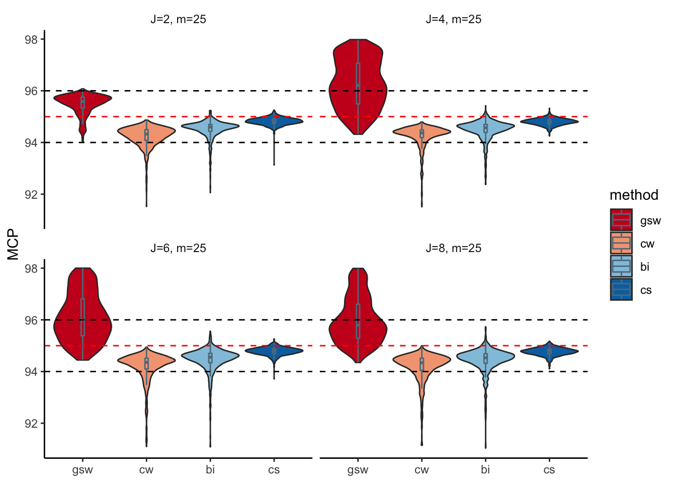
Figure 1: Violin-plots and Boxplots of MCP with m=25

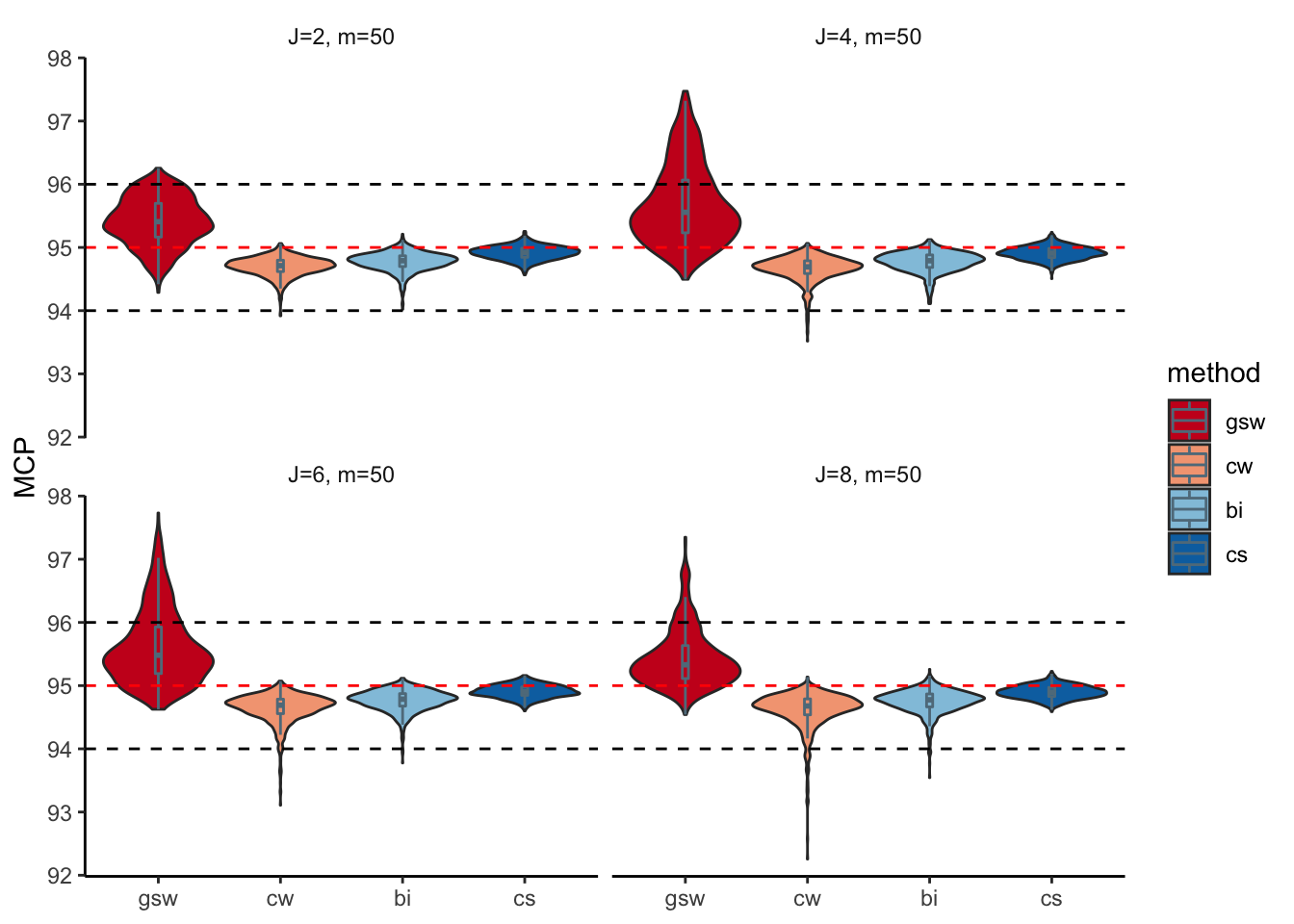
Figure 2: Violin-plots and Boxplots of MCP with m=50

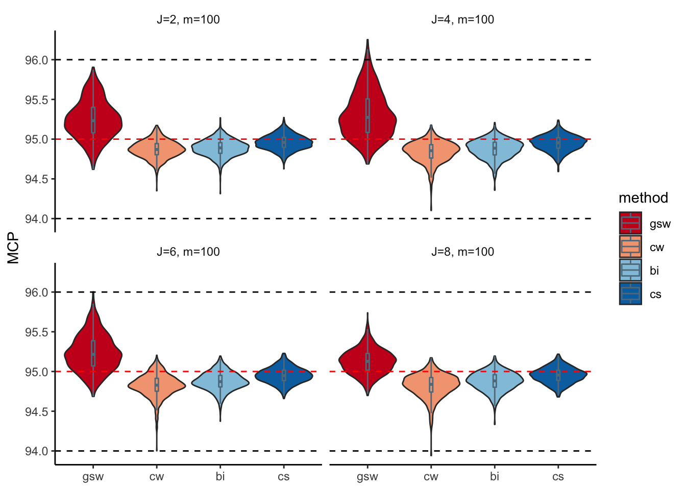
Figure 3: Violin-plots and Boxplots of MCP with m=100

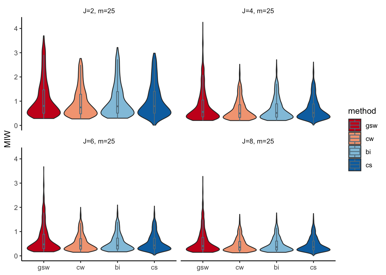
Figure 4: Violin-plots and Boxplots of MIW with m=25

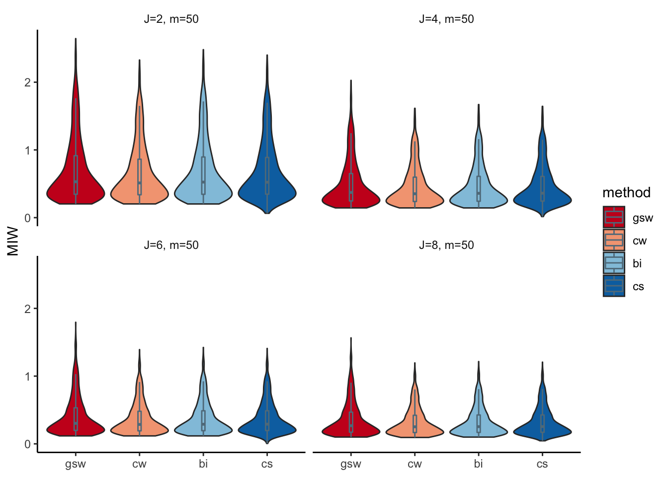
Figure 5: Violin-plots and Boxplots of MIW with m=50

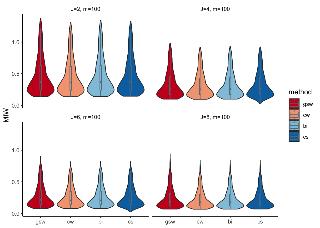
Figure 6: Violin-plots and Boxplots of MIW with m=100

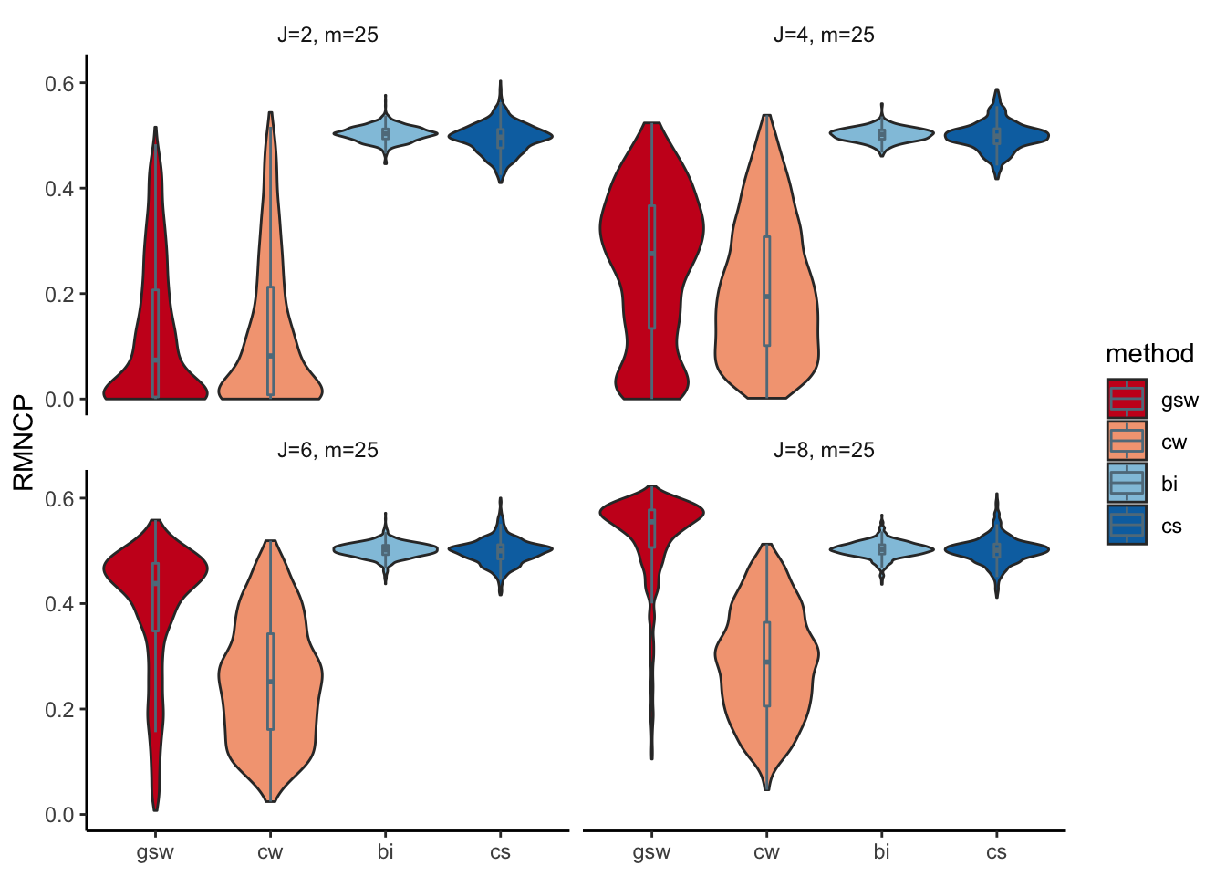
Figure 7: Violin-plots and Boxplots of RMNCP with m=25

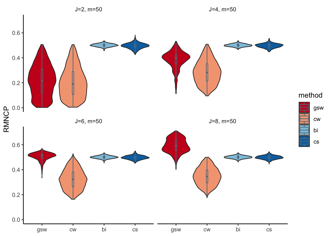
Figure 8: Violin-plots and Boxplots of RMNCP with m=50

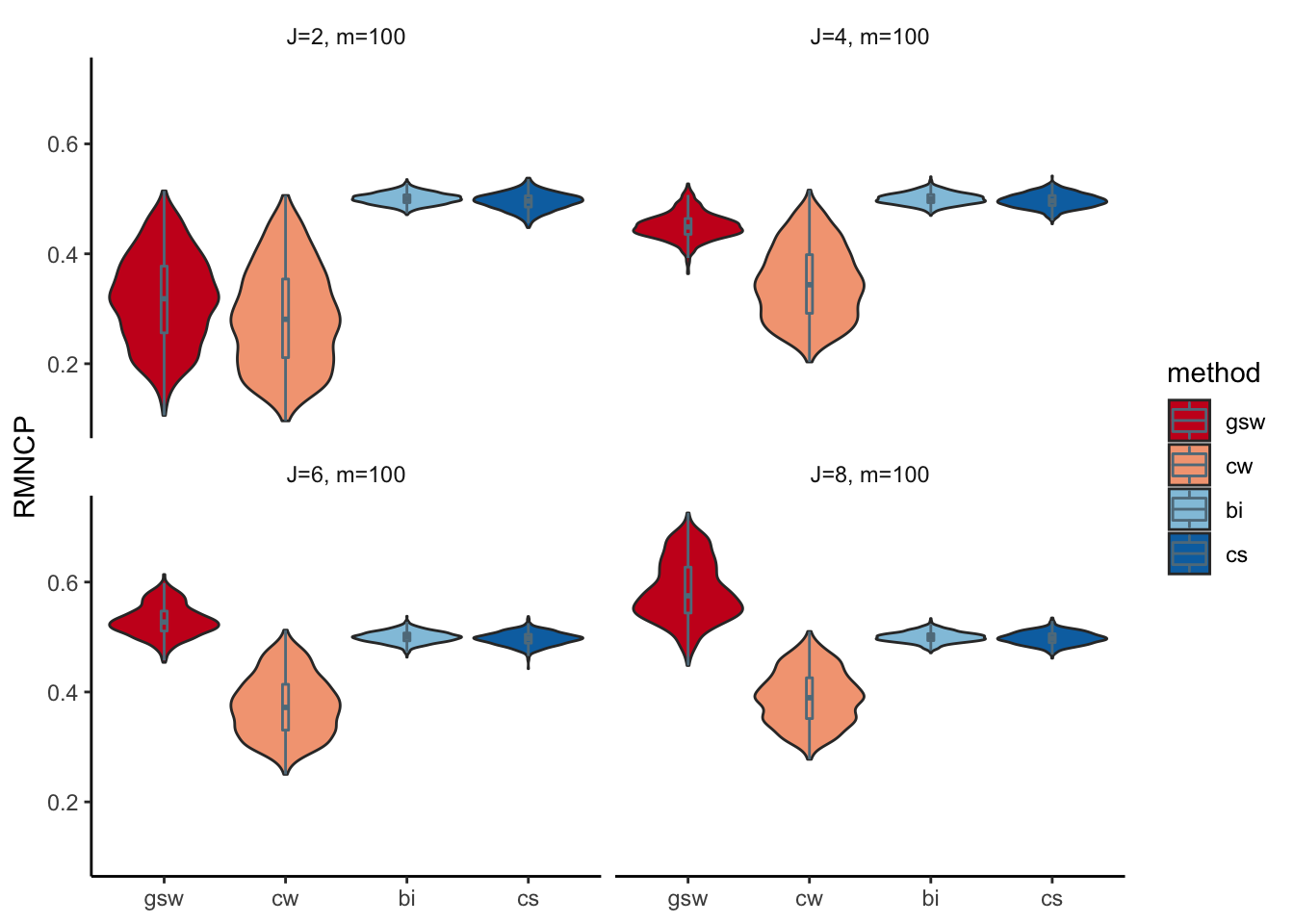
Figure 9: Violin-plots and Boxplots of RMNCP with m=100

6 Real Data Example

We use the double-blinded randomized clinical trial data by Mandel et al. (1982) to illustrate the proposed four CI constructions. In this clinical trial, children who suffer from otitis media with effusion (OME) and have bilateral tympanocentesis are randomly assigned into two groups: amoxicillin or cefaclor, to receive the 14-day treatment  [22]. After the treatment, the number of cured ears are summarized in table 18 with age group as strata.

By applying the four CI constructions in section 4, we obtain the MLEs of parameters based on observed data, shown in Table 19, and the four CI estimators are summarized in Table 20. As shown, all the CIs include 1, which means there is no statistical evidence to reject null hypothesis $H_{0}:\delta_{1}=\delta_{2}=\cdots=\delta_{J}=1$.

Table 18: Frequency of number of OME-free ears after treatment.

	Age group
	$<$2 years		2-5 years		$\geq$6 years
Number of OME-Free ears	Cefactor	Amoxicillin	Cefactor	Amoxicillin	Cefactor	Amoxicillin
0	8	11	6	3	0	1
1	2	2	6	1	1	0
2	8	2	10	5	3	6

Table 18: Table 1. Frequency of number of OME-free ears after treatment. (continued)

Table 19: MlEs of parameters based on observed data.

	Global MlEs			Unconstrained MLEs			Constrained MLEs
Age groups	$\tilde{\pi}_{1}$	$\tilde{\gamma}$	$\tilde{\delta}$	$\hat{\pi}_{1}$	$\hat{\gamma}$	$\hat{\delta}$	$\hat{\pi}_{1{H_{0}}}$	$\hat{\gamma}_{H_{0}}$	$\hat{\delta}_{H_{0}}$
$<$2 years	0.476	0.833	0.480	0.404	0.833	0.8174	0.364	0.833	1
2-5 years	0.612	0.811	0.917	0.625	0.811	-	0.597	0.811	-
$\geq$6 years	0.950	0.947	0.857	0.950	0.947	-	0.864	0.947	-

Table 19: MlEs of parameters based on observed data. (continued)

Table 20: Confidence interval estimation of proportion ratios for the proposed methods.

method	Lower Limit	Upper Limit
Global Weighted Wald (SGW)	0.432	1.000
Profile Likelihood (BI)	0.529	1.047
Complete Wald (CW)	0.548	1.080
Complete Score (CS)	0.529	1.113

Table 20: Confidence interval estimation of proportion ratios for the proposed methods. (continued)

7 Conclusions

Following Dallal’s intraclass correlation model, this article utilizes four confidence interval methods (SGW, CW, BI, CS) to solve the CI construction for proportion ratios of two proportions on stratified bilateral correlated data. In addition, three evaluations indices (MCP, MIW, RMNCP) are proposed to generate the relative comprehensive evaluation for four presented confidence interval methods.

Two Monte Carlo simulation results show that profile likelihood confidence interval with the bisection algorithm (BI) is recommended without considering the conservative performance in small sample size with multiple strata. Meanwhile, the complete MLE-based score confidence interval (CS) method outperforms other CI methods considering all three evaluation indices, which is highly recommended.

However, asymptotic methods might be limited because of poor performance under a small sample size. Future work might consider exact tests to investigate related issues.

8 Appendix

8.1 Information matrix derivation for sample-size weighted global-MLE based wald-type confidence interval (SGW)

The first order differential equations of stratum j are:

$$\frac{\partial l_{j}}{\partial\delta_{j}}=\frac{m_{12j}}{\delta_{j}}+\frac{m_{22j}}{\delta_{j}}+\frac{m_{02j}\,\pi_{1j}\,{\left(\gamma_{j}-2\right)}}{\delta_{j}\,\pi_{1j}\,{\left(\gamma_{j}-2\right)}+1},$$

$$\frac{\partial l_{j}}{\partial\pi_{1j}}=\frac{m_{12j}}{\pi_{1j}}+\frac{m_{21j}}{\pi_{1j}}+\frac{m_{22j}}{\pi_{1j}}+\frac{m_{01j}\,{\left(\gamma_{j}-2\right)}}{\pi_{1j}\,{\left(\gamma_{j}-2\right)}+1}+\frac{\delta_{j}\,m_{02j}\,{\left(\gamma_{j}-2\right)}}{\delta_{j}\,\pi_{1j}\,{\left(\gamma_{j}-2\right)}+1}+\frac{m_{11j}\,{\left(2\,\gamma_{j}-2\right)}}{2\,\pi_{1j}\,{\left(\gamma_{j}-1\right)}},$$

$$\frac{\partial l_{j}}{\partial\gamma_{j}}=\frac{m_{21j}}{\gamma_{j}}+\frac{m_{22j}}{\gamma_{j}}+\frac{m_{11j}}{\gamma_{j}-1}+\frac{m_{12j}}{\gamma_{j}-1}+\frac{m_{01j}\,\pi_{1j}}{\pi_{1j}\,{\left(\gamma_{j}-2\right)}+1}+\frac{\delta_{j}\,m_{02j}\,\pi_{1j}}{\delta_{j}\,\pi_{1j}\,{\left(\gamma_{j}-2\right)}+1}.$$

The second order differential equations of stratum j are:

$$\frac{\partial^{2}l_{j}}{\partial\delta_{j}^{2}}=-\frac{m_{12j}}{\delta_{j}^{2}}-\frac{m_{22j}}{\delta_{j}^{2}}-\frac{m_{02j}\,{\pi_{1j}}^{2}\,{{\left(\gamma_{j}-2\right)}}^{2}}{{{\left(\delta_{j}\,\pi_{1j}\,{\left(\gamma_{j}-2\right)}+1\right)}}^{2}},$$

$$\frac{\partial^{2}l_{j}}{\partial\delta_{j}\partial\pi_{1j}}=\frac{m_{02j}\,{\left(\gamma_{j}-2\right)}}{\delta_{j}\,\pi_{1j}\,{\left(\gamma_{j}-2\right)}+1}-\frac{\delta_{j}\,m_{02j}\,\pi_{1j}\,{{\left(\gamma_{j}-2\right)}}^{2}}{{{\left(\delta_{j}\,\pi_{1j}\,{\left(\gamma_{j}-2\right)}+1\right)}}^{2}},$$

$$\frac{\partial^{2}l_{j}}{\partial\delta_{j}\partial\gamma_{j}}=\frac{m_{02j}\,\pi_{1j}}{\delta_{j}\,\pi_{1j}\,{\left(\gamma_{j}-2\right)}+1}-\frac{\delta_{j}\,m_{02j}\,{\pi_{1j}}^{2}\,{\left(\gamma_{j}-2\right)}}{{{\left(\delta_{j}\,\pi_{1j}\,{\left(\gamma_{j}-2\right)}+1\right)}}^{2}},$$

$$\frac{\partial^{2}l_{j}}{\partial\pi_{1j}\partial\delta_{j}}=\frac{m_{02j}\,{\left(\gamma_{j}-2\right)}}{\delta_{j}\,\pi_{1j}\,{\left(\gamma_{j}-2\right)}+1}-\frac{\delta_{j}\,m_{02j}\,\pi_{1j}\,{{\left(\gamma_{j}-2\right)}}^{2}}{{{\left(\delta_{j}\,\pi_{1j}\,{\left(\gamma_{j}-2\right)}+1\right)}}^{2}},$$

$$\frac{\partial^{2}l_{j}}{\partial\pi_{1j}^{2}}=-\frac{m_{12j}}{{\pi_{1j}}^{2}}-\frac{m_{21j}}{{\pi_{1j}}^{2}}-\frac{m_{22j}}{{\pi_{1j}}^{2}}-\frac{m_{01j}\,{{\left(\gamma_{j}-2\right)}}^{2}}{{{\left(\pi_{1j}\,{\left(\gamma_{j}-2\right)}+1\right)}}^{2}}-\frac{\delta^{2}\,m_{02j}\,{{\left(\gamma_{j}-2\right)}}^{2}}{{{\left(\delta_{j}\,\pi_{1j}\,{\left(\gamma_{j}-2\right)}+1\right)}}^{2}}-\frac{m_{11j}\,{\left(2\,\gamma_{j}-2\right)}}{2\,{\pi_{1j}}^{2}\,{\left(\gamma_{j}-1\right)}},$$

$$\frac{\partial^{2}l_{j}}{\partial\pi_{1j}\partial\gamma_{j}}=\frac{m_{01j}}{{{\left(\pi_{1j}\,{\left(\gamma_{j}-2\right)}+1\right)}}^{2}}+\frac{\delta_{j}\,m_{02j}}{{{\left(\delta_{j}\,\pi_{1j}\,{\left(\gamma_{j}-2\right)}+1\right)}}^{2}},$$

$$\frac{\partial^{2}l_{j}}{\partial\gamma_{j}\partial\delta_{j}}=\frac{m_{02j}\,\pi_{1j}}{\delta_{j}\,\pi_{1j}\,{\left(\gamma_{j}-2\right)}+1}-\frac{\delta_{j}\,m_{02j}\,{\pi_{1j}}^{2}\,{\left(\gamma_{j}-2\right)}}{{{\left(\delta_{j}\,\pi_{1j}\,{\left(\gamma_{j}-2\right)}+1\right)}}^{2}},$$

$$\frac{\partial^{2}l_{j}}{\partial\gamma_{j}\partial\pi_{1j}}\frac{m_{01j}}{{{\left(\pi_{1j}\,{\left(\gamma_{j}-2\right)}+1\right)}}^{2}}+\frac{\delta_{j}\,m_{02j}}{{{\left(\pi_{1j}\,{\left(2\,\delta_{j}-\delta_{j}\,\gamma_{j}\right)}-1\right)}}^{2}},$$

$$\frac{\partial^{2}l_{j}}{\partial\gamma_{j}^{2}}=-\frac{m_{21j}}{{\gamma_{j}}^{2}}-\frac{m_{22j}}{{\gamma_{j}}^{2}}-\frac{m_{11j}}{{{\left(\gamma_{j}-1\right)}}^{2}}-\frac{m_{12j}}{{{\left(\gamma_{j}-1\right)}}^{2}}-\frac{m_{01j}\,{\pi_{1j}}^{2}}{{{\left(\pi_{1j}\,{\left(\gamma_{j}-2\right)}+1\right)}}^{2}}-\frac{\delta^{2}\,m_{02j}\,{\pi_{1j}}^{2}}{{{\left(\delta_{j}\,\pi_{1j}\,{\left(\gamma_{j}-2\right)}+1\right)}}^{2}}.$$

Fisher information of stratum j are:

$$I_{11}^{(j)}=E\left(-\frac{\partial^{2}l_{j}}{\partial\delta_{j}^{2}}\right)=\frac{m_{+2j}}{\delta_{j}^{2}\,{\left(\delta_{j}\,\pi_{1j}\,{\left(\gamma_{j}-2\right)}+1\right)}}-\frac{m_{+2j}}{\delta_{j}^{2}},$$

$$I_{12}^{(j)}=I_{21}^{(j)}=E\left(-\frac{\partial^{2}l_{j}}{\partial\delta_{j}\partial\pi_{1j}}\right)=\-\frac{m_{+2j}\,{\left(\gamma_{j}-2\right)}}{\delta_{j}\,\pi_{1j}\,{\left(\gamma_{j}-2\right)}+1},$$

$$I_{13}^{(j)}=I_{31}^{(j)}=E\left(-\frac{\partial^{2}l_{j}}{\partial\delta_{j}\partial\gamma_{j}}\right)=-\frac{m_{+2j}\,\pi_{1j}}{\delta_{j}\,\pi_{1j}\,{\left(\gamma_{j}-2\right)}+1},$$

$$I_{22}^{(j)}=E\left(-\frac{\partial^{2}l_{j}}{\partial\pi_{1j}^{2}}\right)=\frac{m_{+1j}\,{{\left(\gamma_{j}-2\right)}}^{2}}{\pi_{1j}\,{\left(\gamma_{j}-2\right)}+1}-\frac{{\left(\gamma_{j}-2\right)}\,{\left(m_{+1j}+\delta_{j}\,m_{+2j}\right)}}{\pi_{1j}}-\frac{\delta_{j}^{2}\,m_{+2j}\,{{\left(\gamma_{j}-2\right)}}^{2}}{\pi_{1j}\,{\left(2\,\delta_{j}-\delta_{j}\,\gamma_{j}\right)}-1},$$

$$I_{23}^{(j)}=I_{32}^{(j)}=E\left(-\frac{\partial^{2}l_{j}}{\partial\pi_{1j}\gamma_{j}}\right)=\frac{\delta_{j}\,m_{+2j}}{\pi_{1j}\,{\left(2\,\delta_{j}-\delta_{j}\,\gamma_{j}\right)}-1}-\frac{m_{+1j}}{\pi_{1j}\,{\left(\gamma_{j}-2\right)}+1},$$

$$I_{33}^{(j)}=E\left(-\frac{\partial^{2}l_{j}}{\partial\gamma_{j}^{2}}\right) =\frac{m_{+1j}\,\pi_{1j}}{\gamma_{j}}-\frac{2\,m_{+1j}\,\pi_{1j}}{\gamma_{j}-1}+\frac{m_{+1j}\,{\pi_{1j}}^{2}}{\pi_{1j}\,{\left(\gamma_{j}-2\right)}+1}$$

$$+\frac{\delta_{j}^{2}\,m_{+2j}\,{\pi_{1j}}^{2}}{\delta_{j}\,\pi_{1j}\,{\left(\gamma_{j}-2\right)}+1}+\frac{\delta_{j}\,m_{+2j}\,\pi_{1j}}{\gamma_{j}}-\frac{2\,\delta_{j}\,m_{+2j}\,\pi_{1j}}{\gamma_{j}-1}.$$

and

$$I_{j}=\left[\begin{array}[]{ccc}I_{11}^{(j)}&I_{12}^{(j)}&I_{13}^{(j)}\\ I_{21}^{(j)}&I_{22}^{(j)}&I_{23}^{(j)}\\ I_{31}^{(j)}&I_{32}^{(j)}&I_{33}^{(j)}\end{array}\right]_{3J\times 3J}.$$

Then

$$I_{j}^{-1}=\left(\frac{1}{D^{(j)}}\right)\left(\begin{array}[]{ccc}{\left(I_{22}^{(j)}\,I_{33}^{(j)}-I_{23}^{(j)}\,I_{32}^{(j)}\right)}&-{\left(I_{12}^{(j)}\,I_{33}^{(j)}-I_{13}^{(j)}\,I_{32}^{(j)}\right)}&{\left(I_{12}^{(j)}\,I_{23}^{(j)}-I_{13}^{(j)}\,I_{22}^{(j)}\right)}\\ -{\left(I_{21}^{(j)}\,I_{33}^{(j)}-I_{23}^{(j)}\,I_{31}^{(j)}\right)}&{\left(I_{11}^{(j)}\,I_{33}^{(j)}-I_{13}^{(j)}\,I_{31}^{(j)}\right)}&-{\left(I_{11}^{(j)}\,I_{23}^{(j)}-I_{13}^{(j)}\,I_{21}^{(j)}\right)}\\ {\left(I_{21}^{(j)}\,I_{32}^{(j)}-I_{22}^{(j)}\,I_{31}^{(j)}\right)}&-{\left(I_{11}^{(j)}\,I_{32}^{(j)}-I_{12}^{(j)}\,I_{31}^{(j)}\right)}&{\left(I_{11}^{(j)}\,I_{22}^{(j)}-I_{12}^{(j)}\,I_{21}^{(j)}\right)}\end{array}\right),$$

and

$$D^{(j)}=I_{11}^{(j)}\,I_{22}^{(j)}\,I_{33}^{(j)}-I_{11}^{(j)}\,I_{23}^{(j)}\,I_{32}^{(j)}-I_{12}^{(j)}\,I_{21}^{(j)}\,I_{33}^{(j)}+I_{12}^{(j)}\,I_{23}^{(j)}\,I_{31}^{(j)}+I_{13}^{(j)}\,I_{21}^{(j)}\,I_{32}^{(j)}-I_{13}^{(j)}\,I_{22}^{(j)}\,I_{31}^{(j)}.$$

Then the $cI_{j}^{-1}c^{T}=I_{j}^{-1}{}_{(1,1)}=\left(\frac{1}{D^{(j)}}\right)\left(I_{22}^{(j)}I_{33}^{(j)}-I_{23}^{(j)}I_{32}^{(j)}\right)$

8.2 Information matrix derivation for complete MLE-based Wald-type confidence interval and Score confidence interval

Under the assumption that each stratum has a common ratio of proportions $\delta$, the Fisher information matrix is written as

$$I=\left[\begin{array}[]{ccc}\underset{(1\times 1)}{I_{11}}&\underset{(1\times J)}{I_{12}}&\underset{(1\times J)}{I_{13}}\\ \underset{(J\times 1)}{I_{21}}&\underset{(J\times J)}{I_{22}}&\underset{(J\times J)}{I_{23}}\\ \underset{(J\times 1)}{I_{31}}&\underset{(J\times J)}{I_{32}}&\underset{(J\times J)}{I_{33}}\end{array}\right]$$

where

$$I_{11}=\mathrm{E}\left(-\sum_{j=1}^{J}\frac{\partial^{2}l_{j}}{\partial\delta^{2}}\right)=\sum_{j=1}^{J}\frac{m_{+2j}}{\delta^{2}\,{\left(\delta\,\pi_{1j}\,{\left(\gamma_{j}-2\right)}+1\right)}}-\frac{m_{+2j}}{\delta^{2}},$$

$$I_{12}=I_{21}^{T} =\left[\mathrm{E}\left(-\frac{\partial^{2}l_{1}}{\partial\delta\partial\pi_{11}}\right),\mathrm{E}\left(-\frac{\partial^{2}l_{2}}{\partial\delta\partial\pi_{12}}\right),\ldots,\mathrm{E}\left(-\frac{\partial^{2}l_{J}}{\partial\delta\partial\pi_{1J}}\right)\right]$$

$$=\left[I_{12}^{(1)},I_{12}^{(2)},\ldots,I_{12}^{(J)}\right]$$

Where

$$I_{12}^{(j)}=\-\frac{m_{+2j}\,{\left(\gamma_{j}-2\right)}}{\delta\,\pi_{1j}\,{\left(\gamma_{j}-2\right)}+1},$$

$$I_{13}=I_{31}^{T} =\left[\mathrm{E}\left(-\frac{\partial^{2}l_{1}}{\partial\delta\partial\gamma_{1}}\right),\mathrm{E}\left(-\frac{\partial^{2}l_{2}}{\partial\delta\partial\gamma_{2}}\right),\ldots,\mathrm{E}\left(-\frac{\partial^{2}l_{J}}{\partial\delta\partial\gamma_{J}}\right)\right]$$

$$=\left[I_{13}^{(1)},I_{13}^{(2)},\ldots,I_{13}^{(J)}\right]$$

where

$$I_{13}^{(j)}=-\frac{m_{+2j}\,\pi_{1j}}{\delta\,\pi_{1j}\,{\left(\gamma_{j}-2\right)}+1}.$$

$$I_{22}=\operatorname{diag}\left\{\mathrm{E}\left(-\frac{\partial^{2}l_{j}}{\partial\pi_{1j}^{2}}\right)\right\}=\left(\begin{array}[]{llll}I_{22}^{(1)}&&&\\ &I_{22}^{(2)}&&\\ &&\ddots&\\ &&&I_{22}^{(J)}\end{array}\right),\quad j=1,2,\ldots,J$$

where

$$I_{22}^{(j)}=\frac{m_{+1j}\,{{\left(\gamma_{j}-2\right)}}^{2}}{\pi_{1j}\,{\left(\gamma_{j}-2\right)}+1}-\frac{{\left(\gamma_{j}-2\right)}\,{\left(m_{+1j}+\delta\,m_{+2j}\right)}}{\pi_{1j}}-\frac{\delta^{2}\,m_{+2j}\,{{\left(\gamma_{j}-2\right)}}^{2}}{\pi_{1j}\,{\left(2\,\delta-\delta\,\gamma_{j}\right)}-1},$$

$$I_{32}^{T}=I_{23}=\operatorname{diag}\left\{E\left(-\frac{\partial^{2}I_{j}}{\partial\pi_{1j}\gamma_{j}}\right)\right\}=\left(\begin{array}[]{llll}I_{23}^{(1)}&&&\\ &I_{23}^{(2)}&&\\ &&\ddots&\\ &&&I_{23}^{(J)}\end{array}\right),\quad j=1,2,\ldots,J$$

$$I_{23}^{(j)}=\frac{\delta\,m_{+2j}}{\pi_{1j}\,{\left(2\,\delta-\delta\,\gamma_{j}\right)}-1}-\frac{m_{+1j}}{\pi_{1j}\,{\left(\gamma_{j}-2\right)}+1},$$

$$I_{33}=\operatorname{diag}\left\{\mathrm{E}\left(-\frac{\partial^{2}l_{j}}{\partial\gamma_{j}^{2}}\right)\right\}=\left(\begin{array}[]{llll}I_{33}^{(1)}&&&\\ &I_{33}^{(2)}&&\\ &&\ddots&\\ &&&I_{33}^{(J)}\end{array}\right),\quad j=1,2,\ldots,J$$

where

$$I_{33}^{(j)} =\frac{m_{+1j}\,\pi_{1j}}{\gamma_{j}}-\frac{2\,m_{+1j}\,\pi_{1j}}{\gamma_{j}-1}+\frac{m_{+1j}\,{\pi_{1j}}^{2}}{\pi_{1j}\,{\left(\gamma_{j}-2\right)}+1}$$

$$+\frac{\delta^{2}\,m_{+2j}\,{\pi_{1j}}^{2}}{\delta\,\pi_{1j}\,{\left(\gamma_{j}-2\right)}+1}+\frac{\delta\,m_{+2j}\,\pi_{1j}}{\gamma_{j}}-\frac{2\,\delta\,m_{+2j}\,\pi_{1j}}{\gamma_{j}-1}.$$

Then

$$CI^{-1}C^{T}=I^{-1}_{(1,1)}=\left(I_{11}-\left[\begin{array}[]{ll}I_{12}&I_{13}\end{array}\right]\left[\begin{array}[]{ll}I_{22}&I_{23}\\ I_{32}&I_{33}\end{array}\right]^{-1}\left[\begin{array}[]{l}I_{21}\\ I_{31}\end{array}\right]\right)^{-1}$$

References

- [1] John J Gart and Jun-mo Nam. Approximate interval estimation of the ratio of binomial parameters: a review and corrections for skewness. Biometrics, pages 323–338, 1988.
- [2] PAR Koopman. Confidence intervals for the ratio of two binomial proportions. Biometrics, pages 513–517, 1984.
- [3] Kristin Sainani. The importance of accounting for correlated observations. PM&R, 2(9):858–861, 2010.
- [4] Bernard Rosner. Statistical methods in ophthalmology: an adjustment for the intraclass correlation between eyes. Biometrics, 38, March 1982.
- [5] Allan Donner. Statistical methods in ophthalmology: an adjusted chi-square approach. Biometrics, 45, 1989.
- [6] Xuan Peng, Chang Liu, Song Liu, and Chang-Xing Ma. Asymptotic confidence interval construction for proportion ratio based on correlated paired data. Journal of Biopharmaceutical Statistics, 29(6), 2019.
- [7] Nian-Sheng Tang, Hui-Qiong Li, Man-Lai Tang, and Jie Li. Confidence interval construction for the difference between two correlated proportions with missing observations. Journal of Biopharmaceutical Statistics, 26(2):323–338, 2016.
- [8] Man-lai Tang, Xinjie He, and Guoliang Tian. A confidence interval approach for comparative studies involving binary outcomes in paired organs. Communications in Statistics—Simulation and Computation, 42(2), 2013.
- [9] Zhengyu Yang, Guo-Liang Tian, Xiaobin Liu, and Chang-Xing Ma. Simultaneous confidence interval construction for many-to-one comparisons of proportion differences based on correlated paired data. Journal of Applied Statistics, 48(8):1442–1456, 2021.
- [10] Weizhen Wang and Guogen Shan. Exact confidence intervals for the relative risk and the odds ratio. Biometrics, 71(4):985–995, 2015.
- [11] Zhiming Li and Changxing Ma. Statistical inference for odds ratio of two proportions in bilateral correlated data. Axioms, 11(10):502, 2022.
- [12] Yanbo Pei, Man-Lai Tang, Weng-Kee Wong, and Jianhua Guo. Confidence intervals for correlated proportion differences from paired data in a two-arm randomised clinical trial. Statistical Methods in Medical Research, 21(2), 2012.
- [13] Gerade E. Dallal. Paired bernoulli trials. Biometrics, 44, March 1988.
- [14] Yuqing Xue and Chang-Xing Ma. Interval estimation of proportion ratios for stratified bilateral correlated binary data. Statistical Methods in Medical Research, 29(7), 2020.
- [15] Tingting Zhuang, Guo-Liang Tian, and Chang-Xing Ma. Confidence intervals for proportion ratios of stratified correlated bilateral data. Journal of Biopharmaceutical Statistics, 29(1), 2019.
- [16] Xi Shen, Chang-Xing Ma, Kam C Yuen, and Guo-Liang Tian. Common risk difference test and interval estimation of risk difference for stratified bilateral correlated data. Statistical Methods in Medical Research, 28(8), 2019.
- [17] Nian-Sheng Tang, Shi-Fang Qiu, Man-Lai Tang, Guang-Yong Zou, and Dan Yu. Simultaneous confidence intervals of risk differences in stratified paired designs. Journal of Biopharmaceutical Statistics, 23(2):361–377, 2013.
- [18] Robert G Newcombe. Improved confidence intervals for the difference between binomial proportions based on paired data. Statistics in Medicine, 17, 1998.
- [19] Robert G Newcombe. Measures of location for confidence intervals for proportions. Communications in Statistics-Theory and Methods, 40(10):1743–1767, 2011.
- [20] Robert G Newcombe. Two-sided confidence intervals for the single proportion: comparison of seven methods. Statistics in medicine, 17(8):857–872, 1998.
- [21] Robert G Newcombe. Confidence intervals for the mean of a variable taking the values 0, 1 and 2. Statistics in medicine, 22(17):2737–2750, 2003.
- [22] Ellen M Mandel, Charles D Bluestone, Howard E Rockette, Mark M Blatter, Keith S Reisinger, Frederick P Wucher, and James Harper. Duration of effusion after antibiotic treatment for acute otitis media: comparison of cefaclor and amoxicillin. Pediatric infectious disease, 1(5):310–316, 1982.