Dynamic Prioritization and Adaptive Scheduling using Deep Deterministic Policy Gradient for Deploying Microservice-based VNFs

Abstract

The Network Function Virtualization (NFV)- Resource Allocation (RA) problem is NP-Hard. Traditional deployment methods revealed the existence of a starvation problem, which the researchers failed to recognize. Basically, starvation here, means the longer waiting times and eventual rejection of low-priority services due to a ‘time out’. The contribution of this work is threefold: a) explain the existence of the starvation problem in the existing methods and their drawbacks, b) introduce ‘Adaptive Scheduling’ (AdSch) which is an ‘intelligent scheduling’ scheme using a three-factor approach (priority, threshold waiting time, and reliability), which proves to be more reasonable than traditional methods solely based on priority, and c) a ‘Dynamic Prioritization’ (DyPr), allocation method is also proposed for unseen services and the importance of macro- and micro-level priority. We presented a zero-touch solution using Deep Deterministic Policy Gradient (DDPG) for adaptive scheduling and an online- Ridge Regression (RR) model for dynamic prioritization. The DDPG successfully identified the ‘Beneficial and Starving’ services, efficiently deploying twice as many low-priority services as others, reducing the starvation problem. Our online-RR model learns the pattern in less than 100 transitions, and the prediction model has an accuracy rate of more than 80%.

I Introduction

Although the fifth generation of mobile networks (5G) is presently providing the fundamental support for the Internet of Everything (IoE) and Ultra-Reliable Low Latency Communications (URLLC), it is debatable if the current 5G systems can smoothly handle applications like Digital Twin (DT), connected robotics, autonomous systems, Augmented Reality (AR)/ Virtual Reality (VR)/ Mixed Reality (MR), and Blockchain and Trust technologies  [1, 2]. These upcoming applications are envisioned to request services with stringent standards, such as high reliability, low latency, and significant data rates [1]. Due to this debate, there has been a significant research progress towards sixth generation of mobile networks (6G).The 6G must be tailored to support the upcoming service types like Computation Oriented Communications (COC), Contextually Agile eMBB Communications (CAeC), and Event Defined uRLLC (EDuRLLC) in addition to enhanced Mobile Broadband (eMBB), URLLC, and massive Machine Type Communications (mMTC) services [3].

There are several initiatives on both the access and the network side to facilitate the transition towards the 6G. On the network side, the NFV architecture, introduced in 2012 [4], is pushing towards the microservices-based architecture [5, 6]. The NFV framework virtualizes the Network Functions from their dedicated proprietary substrate appliances by allowing them to run as softwarized NFs (say, Virtual Network Functions) on commodity hardware. This enables freedom, flexibility, and agility for VNFs to migrate from one server to another in response to dynamic variations in resource demand. Although NFV is a promising technology, it can be challenging when various applications coexist, and simultaneously the underlying infrastructure requires guaranteed resources for all the arriving Service Function Chaining (SFC). This is an NP-Hard problem and is known as the NFV-RA. In this type of NFV-RA, due to the affinity and anti-affinity constraints, the complexity grows further, hindering effortless software updates and routine maintenance. To address this, microservices offer an increased degree of freedom in the scalability, flexible upgrades and maintenance of VNFs. This cutting-edge ‘NFV-RA + Microservies’ strategy ppromises to offer a solution (theoretically) closer to the optimum, despite having an intensified design and deployment complexity. In [7] we provided a detailed analysis of this approach and the criteria for executing dynamic decomposition, of which, Section III-D provides an overview.

We examine a deeper analysis of the criteria for dynamically prioritizing the online SFCs, the merits of embedding an SFC over others and the significance of admission control. Most research to date has concentrated exclusively on deploying SFCs using First-in-First-out (FIFO). Realistically, not all SFCs fall under the same priority group and cannot be addressed equally. The traditional method, FIFO, failed to recognize and give emergency SFCs higher preference than non-emergency ones, causing the rejection of highly critical SFCs. In a modified approach, the priority-based approach is established to prefer the high-priority SFCs first over the lower ones [8, 9], which overcomes the FIFO drawback. Nevertheless, this introduced ‘starvation for lower-priority services, causing a significant biasness in the system - an unfair design to the users. To dismiss this biasness, the critical SFC should not be classified based on priority levels but rather with other essential attributes. Thus, requiring an ‘intelligent fair system’. Moreover, with the lack of requested service information, predicting the types of arriving SFCs and their priority level will be challenging considering future communications. Thus, we need to dynamically classify the online services.

In this paper, to provide seamless support to more realistic services for future networks, we propose a DyPr and an AdSch module for arriving SFCs using the RR model and DDPG approach, respectively, to diminish the ‘Starvation’ situation and provide a fair scheduling principle. Our proposed DDPG-based algorithm identifies and understands the importance of embedding the ‘Beneficial SFC’ or ‘Starving SFC’ over others. The criteria and methods for assessing the priority of the online service have also not been specified in the literature; instead, a static approach has been adopted. Thus we have first proposed a standard for estimating the priority of an SFC dynamically by using the Machine Learning (ML) technique. Using the achieved priority and other Quality of Service (QoS) attributes, we trained our DDPG-based model to rank the arriving SFCs based on their urgency and requirements. Based on the SFC’s rank, the rescheduling for deployment occurs; later on, the SFC has to go through the admission control module, which provides permission or rejection for deployment based on the waited time by the SFCs in the queue. In summary, the main contributions of this paper are:

• Establish a dynamic priority estimation criteria for all the online services using the RR model.

• Develop a DDPG-based framework for recognizing and understanding the importance of preferring an SFC (say, ‘Beneficial and Starving SFC’) over others.

• Establish an admission control approach, based on the SFC’s waiting time in the queue before being deployed.

• Adapting the deep Q-Learning (QL) model along with microserives concept for VNF embedding.

II Literature review

To meet the Service Level Agreements of next generation networks, NFV has received a lot of attention. The majority of the research has focused on the placement of arriving SFCs in a FIFO fashion. For instance, [10, 11] formulated the problem based on the exact optimization method; however, the solutions are delivered using heuristic or meta-heuristic models due to the high computational cost. ML techniques are commonly proposed as an effective technique for handling complicated problems like NFV-RA. Authors in [12, 13, 14, 15, 16] proposed reinforcement learning-based approaches. In a realistic scenario, each service has its own level of importance based on its type and requirements. Following the FIFO technique can cause failure in deploying emergency services over best-effort ones. Methods that classify SFCs as either Premium (Pr) or Best-Effort (BE), constantly prioritizes Pr services over the BE ones, resulting in severe service deprivation for low-priority services [8]. [17] and [18] demonstrated the effectiveness of mapping the services depending on the priority of VNFs. The authors of [17] discuss three types of priority: per-service, per-VNF, and per-flow, where service prioritization is based on the delay attribute and per VNF priority is assigned randomly. This is an iterative process that adjusts the solution after each iteration, which is not scalable considering future requirements. Also the predefined number of flows that a VNF can handle, ignores the operational dynamics.

Priority-based scheduling and deployment is still an issue requiring an ‘intelligent’ system to dynamically establish the online service priority and re-schedule the services according to the urgency and benefit. Researchers have proposed Integer Linear Program (ILP) or heuristic models in the literature, which are either computationally costly or produce sub-optimal solutions. To overcome this drawback, we propose ML-based algorithms to dynamically assign priority to online services and train the model to re-arrange the scheduling queue according to the needs.

III System Model

The physical topology is modelled as a directed graph $\textbf{G}=(\textbf{H},\textbf{N})$, where $\textbf{H}=[\textbf{h}_{0},\ldots,\textbf{h}_{|H|-1}]$ and $\textbf{N}=[\textbf{n}_{0},\ldots,\textbf{n}_{|N|-1}]$ represent the set of physical nodes (say high-volume servers) and physical links of the topology, respectively. Each physical node $\textbf{h}_{x^{\prime}}=[h_{x^{\prime},0},\ldots,h_{x^{\prime},J_{node}-1}]$ denotes the amount of available nodal resources like CPU core, RAM, etc, and $J_{node}$ is the number of nodal resource types indexed from $0,1,\ldots,J_{node}-1$. Similarly, each physical link $\textbf{n}_{y^{\prime}}=[n_{y^{\prime},0},\ldots,n_{y^{\prime},J_{link}-1}]$ signifies the amount of link resources like bandwidth, latency, etc. $J_{link}$ stands for the number of link resource types, the available resource for physical link. The VNF-Forwarding Graph (VNF-FG) or SFC (${\Psi}$) is represented as a directed graph $\textbf{G}_{\Psi}^{\prime}=(\textbf{V}_{\Psi},\textbf{B}_{\Psi})$ with the set of VNFs ($\textbf{V}_{\Psi}=[\textbf{v}_{\Psi,0},\ldots,\textbf{v}_{\Psi,|V|-1}]$) and Virtual Links ($\textbf{B}_{\Psi}=[\textbf{b}_{\Psi,0},\ldots,\textbf{b}_{\Psi,|b|-1}]$) , that delivers an end-to-end service. Deploying these graphs onto the physical topology is termed as the VNF-FG Embedding (VNF-FGE) problem. Each VNF ($\textbf{v}_{\Psi,x}=[r_{\Psi,x,0},\ldots,r_{\Psi,x,J_{node}-1}]$) and VL ($\textbf{b}_{\Psi,y}=[l_{\Psi,y,0},\ldots,l_{\Psi,y,J_{link}-1}]$) comprises of set of requested resources like CPU core, delay, bandwidth etc. The computing resources initialization in most related works, is done in a random manner, disregarding the high correlation between the CPU core and RAM. This work outlines the link between the CPU core and RAM as in [19]. In addition, we also considered delay, jitters, packet loss, reliability and threshold waiting time as some of the QoS attributes, thus making the $J_{node}=6$ in our case. Similarly, $J_{link}=2$ in our studies, considering latency and bandwidth.

III-A Dynamic Prioritization

A major drawback of commonly-used methods of binary classification of services into Pr and BE is that, the pre-determined priority levels for the arriving services are randomly allocated and the co-relation between the service requirements and priority are ignored. In a realistic scenario, the allocation of service priority should be based on various factors of QoS, flow type, etc. Determining the priority levels for the existing or well-aware services is trivial. The complexity induces when future communications system expects frequent unseen ‘short-lived’ services with instant placement requirements. To fulfil this need, an intelligent and DyPr model is anticipated rather than a static or conventional method. In the DyPr model, we investigate the relationship between the requested QoS factors of the arriving service and, based on it, a dynamic priority level is assigned. This problem is viewed as a multiple regression task with various independent variables $A[0]\dots A[p]$ (like QoS factors with $p$ as the number of factors), to predict a dependent continuous variable $Y^{\prime}$ as referred in Eqn. (1). Here $W$ and $B$ are the regression coefficient and residual term respectively, which are learned during the training. The adopted model discovers the linearity between the dependent and independent variables. In our case, these independent variables are threshold jitters, delay, and packet loss, which a service can tolerate, and the dependent variable denotes the appropriate priority level. However, the multiple regression data suffers from multi-colinearity, which causes the estimation of regression coefficients to be inaccurate. As a result, its existence reduces the model’s performance by causing the predicted value to differ significantly from the actual value. One way to diminish this is by adopting the RR model, which performs L2 regularization, due to which the model is more restricted and causes less over-fitting [20]. The objective is to minimize the cost function mentioned in (2), where $M$ is the number of samples (services per run), $Y_{\Psi}$ is the actual value. The $\lambda$ (penalty term) regularizes the coefficients in such a way that the optimization function is penalized if the coefficients assume high values.

$$\footnotesize Y^{\prime}_{\Psi}=W[0]\times A_{\Psi}[0]+\dots+W[p]\times A_{\Psi}[p]+B$$ (1)

$$\footnotesize\sum_{\Psi=0}^{M}(Y_{\Psi}-Y^{\prime}_{\Psi})^{2}=\sum_{\Psi=1}^{M}(Y_{\Psi}-\sum_{j=0}^{p}W_{j}\times A_{\Psi,j})^{2}+\lambda\sum_{j=0}^{p}W_{j}^{2}$$ (2)

The RR model is supervised learning, which uses pre-existing datasets for training purposes. Our study evaluates the model’s performance for future unseen services; hence, we assume no helpful service information is available to us. The traditional RR model would not provide enough support due to the lack of sufficient datasets. To support the dynamism, we have modified it by adding an observation phase before the learning phase. This helps in constructing our training datasets, making an ‘Online-RR’ model. In the observation phase, due to the unavailability of service information, the model saves (observes) the online services in a memory buffer until the minimal transitions is achieved to begin the training phase. During this time, the allocation of priority is performed uniformly. Later, once the saved transition threshold is surpassed, the learning phase starts, which uses the current and saved transitions for model training. These saved transitions (batch transitions) are selected randomly from the memory to avoid any chance of overfitting (co-relation between the transitions). The model’s accuracy is checked periodically. Once the model reaches the desired accuracy, the trained model state changes from ‘Train’ to ‘Predict’. The overview of DyPr is shown in Fig. 1. Moreover, this model was chosen after a thorough evaluation of model performances using several methodologies, including Artificial Neural Network (ANN) and Lasso. Of all the models, the online-RR model outperformed expectations. This model is constructed with an envision to support future unseen services by introducing a zero-touch cognitive system.

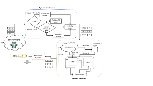
Figure 1: Overview of the DyPr scheme.

Traditionally, the services are categorized into two cardinalities, which diminishes the value of services relative to one another within a class. Most research has ignored the intra-class priority aspect; however, given the future demands, it should be considered. To overcome this, a service priority is ranked between 0.0 to 1.0, with 0.0 represents the least essential service, and 1.0 being the most crucial. Each priority level is expressed in macro-class priority and micro-class priority. While the micro-class priority establishes the priority status inside a class, the macro-class priority categorizes the class to which it belongs. For example, the priority of SFC A and SFC B is 0.79 and 0.72, respectively. Though both the SFCs belong to the same class (i.e., macro-class is 7), SFC A with a micro-class as 9 will be prioritized over the SFC B with a micro-class as 2, due to the higher value. This delivers more details about the importance of services within the class, which is beneficial, especially for time-Sensitive or critical applications and for the adaptive scheduling phase. Therefore, in our work, the DyPr is considered as a Regression model rather than classification.

III-B Adaptive Scheduling

Conventionally, high-priority services are preferred over others, leaving the low-priority services to wait for extended periods of time, resulting in their starvation. This highlights the second drawback of conventional binary classification of services. A biased scheduling system, which raises the questions like, ‘Can the priority attribute be the most effective scheduling decision-making factor?’ ‘Will the decision be more optimal by considering additional factors, such as service waiting time or reliability?’ In a search for an unbiased scheduling system, we have proposed an intelligent Adaptive Scheduling module using the DDPG approach. This approach weighs more than one factor and provides an optimal decision. Let us say, that a high-priority SFC A has a higher waiting threshold than a lower-priority SFC B (which is about to expire soon). According to the traditional model, SFC A will be selected, ignoring the SFC B to expire, affecting the Quality of Experience (QoE). However, our model, which considers more than one factor, prefers SFC B over SFC A, understanding that there will not be any negative impact on SFC A if it waits in a queue a little longer, providing scheduling optimality.

DDPG is an actor-critic Reinforcement Learning (RL) model, trained to identify ‘Beneficial and Starving’ services based on 3-factors: Threshold Waiting Time (TWT) $(T)$, Reliability $(\Gamma)$, and Priority $(P)$ of the service. The state-space for the requested service $\Psi$ is represented as $(T_{\Psi},\Gamma_{\Psi},P_{\Psi})$. Based on these factors, the DDPG agent determines a rank for each service (i.e., action-space $(A_{\Psi})$), indicating the significance of deploying the service. With a higher rank, the necessity to deploy the service is significant, resulting in a rank-based scheduling method. In order to train the DDPG model, an appropriate reward function is essential since it provides feedback to the agent based on the given action’s effectiveness. Equation (3) describes the reward function $R(\cdot)$, which comprises two parts: Beneficial-cost $(\Upsilon)$ and Starvation-cost $(\Phi)$, providing a trade-off between the high-priority, starvation, and high-reliable services. The $R(\cdot)$ is a point-based function; depending upon the significance of factors, the reward points $(\theta_{pts})$ are scaled, as in Eqns. (4) and (5), where $n(\cdot)$ is the normalized function.

$$\footnotesize R(\Psi)=\Upsilon_{\Psi}+\Phi_{\Psi},$$ (3)

$$\footnotesize\Upsilon_{\Psi}=[(1-n(T_{\Psi})\times\theta_{pts})+(\Gamma_{\Psi}\times\theta_{pts})+(P_{\Psi}\times\theta_{pts})],$$ (4)

$$\footnotesize\Phi_{\Psi}=\zeta_{\Psi}\times\theta_{pts},$$ (5)

$$\footnotesize\zeta_{\Psi}=\begin{cases}\alpha(1-\epsilon)^{\kappa},&\text{if }Z_{\Psi}=1\\ 0,&\text{otherwise},\end{cases}$$ (6)

$$\footnotesize Z_{\Psi}=\begin{cases}1,&\text{if }P_{\Psi}\leq 0.2\\ 0,&\text{otherwise},\end{cases}$$ (7)

Equation (5) introduces the biasness to diminish the starvation issue, where $\zeta_{\Psi}$ represents the starvation factor, which decays exponentially with the SFC’s rank. According to Eqn. (7), our algorithm determines if the arriving service qualifies as a ‘Potential Starving’ service or not. On affirmative, the algorithm checks its placement position $\kappa$ in the adaptive scheduling queue, which impacts the starvation cost. $\kappa$ is determined using the exponential decay formula, with $\alpha$ as 1 and decay rate ($1-\epsilon$) as 0.1. The decay rate induces greediness in the system when the service is positioned at the beginning by giving higher rewards than others. Thus, making the agent position the starving services at the beginning.

III-C Admission Control

After achieving an optimal scheduling queue, we constructed an admission-control model to evaluate the extent to which the ‘Potential Starving’ and ‘High-priority’ services are deployed before expiration. This determines the trade-off between starvation and traditionally-preferred services. When a service is under placement, the waiting period $(\Delta)$ for the reminder services is recorded, which is illustrated in a 2-D matrix as below. A scheduling queue, for instance, is $[SFC_{0},SFC_{1},SFC_{2},SFC_{3}]$. When $SFC_{0}$ is placed, the remainder services’ waiting span is $x_{0}$, which is the deployment time of $SFC_{0}$. With the deployment of $SFC_{1}$, the waiting time for $SFC_{2}$ and $SFC_{3}$ is increased by $x_{1}$ and so on. $\Delta_{\Psi,\Psi}$ depicts the total waited time by the service $\Psi$ in the queue.

$$\scriptsize\Delta=\bordermatrix{&SFC_{0}&SFC_{1}&SFC_{2}&SFC_{3}\cr SFC_{0}&\Delta_{0,0}&\Delta_{0,1}&\Delta_{0,2}&\Delta_{0,3}\cr SFC_{1}&\Delta_{1,0}&\Delta_{1,1}&\Delta_{1,2}&\Delta_{1,3}\cr SFC_{2}&\Delta_{2,0}&\Delta_{2,1}&\Delta_{2,2}&\Delta_{2,3}\cr SFC_{3}&\Delta_{3,0}&\Delta_{3,1}&\Delta_{3,2}&\Delta_{3,3}}\qquad$$

$$\scriptsize\Delta=\bordermatrix{&SFC_{0}&SFC_{1}&SFC_{2}&SFC_{3}\cr SFC_{0}&0&x_{0}&x_{0}&x_{0}\cr SFC_{1}&0&x_{0}&x_{0}+x_{1}&x_{0}+x_{1}\cr SFC_{2}&0&x_{0}&x_{0}+x_{1}&x_{0}+x_{1}+x_{2}\cr SFC_{3}&0&x_{0}&x_{0}+x_{1}&x_{0}+x_{1}+x_{2}}\qquad$$

To initiate the placement, the service must satisfy the requirement as in Eqn. (8).

$$\footnotesize\Xi_{\Psi}=\begin{cases}1,&\text{if }\Delta_{\Psi,\Psi}\leq T_{\Psi}\\ 0,&\text{otherwise},\end{cases}$$ (8)

III-D VNF-FGE Problem Formulation

Result of [7] show that the Double Deep Q Learning (DDQL) model solves the NFV-RA problem efficiently, intending to embed maximum SFCs onto the substrate network under certain defined constraints. In [7] we considered the physical topology as an environment comprised of high-volume servers. Each VNF- Forwarding Graph (FG) and its resource requirements are represented as state-space ($S$). The amount of physical nodes/servers present in the topology is described as the action-space ($A$). The Local reward function (i.e., the Eqn. (13) in [7]) has been modified as Eqn. (9) , which is constructed based on the four attributes:

1. $R_{quality,y}$, the quality of the selected node ($y$) for deploying the VNF, ($x$) is the ratio of available resources ($Ar_{y}$) in the node to the initialized resources ($Ir_{y}$), as in Eqn. (11). The availability of resources in a physical node determines its quality.

   $$\footnotesize L_{reward}(x)=\begin{cases}\bm{R_{vnf}},&\text{if }\Phi_{x}^{y}=1\\ P^{pt}_{vnf},&\text{otherwise}\end{cases}$$ (9)

   $$\footnotesize\bm{R_{vnf}}=R_{quality,y}+R_{priority}+R_{rel}+R_{placement}$$ (10)

   $$\footnotesize R_{quality,y}=\frac{Ar_{y}}{Ir_{y}}\times R^{pt}_{vnf}$$ (11)

   $$\footnotesize R_{priority}=P_{\Psi}\times R^{pt}_{vnf}$$ (12)

   $$\footnotesize R_{rel}=\Gamma_{\Psi}\times R^{pt}_{vnf}$$ (13)

   $$\footnotesize R_{placement}=J^{x}_{y}\times R^{pt}_{vnf}$$ (14)

2. Based on the service priority ($R_{priority}$), as in Eqn. (12).

3. Based on the requested service reliability ($R_{rel}$), as Eqn. (13).

4. Time taken by the DDQL model to find an appropriate node for the placement ($J^{x}_{y}$), Eqn. (14) represents the placement reward function ($R_{placement}$).

Algorithm 1 describes the overall model.

1Initialize DDPG Model: Critic, Actor, Target Critic, Target Actor Networks, DDPG Replay Buffer$B_{DDPG}$

2 Initialize RR Memory Buffer $B_{RR}$

3 foreach episode i = 1… epi do

4       Reset the Environment

5       Initialize substrate node resource $R_{H}$, substrate link $R_{N}$

6       Received arriving T services

7       while for all T services do

8             Using DyPr method; online-RR model

9             if status = ”Train” then

10                  if Transition $<$ Threshold Transition then

11                        Priority is selected randomly

12                  else

13                        Online-RR model gets trained

14                   end if

15                  

16            else

17                  Prediction: using Trained model

18             end if

19            

20            Using AdSch method; DDPG model

21             Achieve the Rank for each services

22            

23       end while

24      Sort the T service in ascending order (T’), according to achieved rank

25       foreach time-step t’ = 1…T’ do

26             Admission Control

27             Deployment initiate

28            

29       end foreach

30      

31 end foreach

Algorithm 1 DyPr and AdSch

IV Simulation results

In this section, the effectiveness of the DDPG and RR models for AdSch and DyPr are examined under various conditions, for NetRail (7 nodes, 10 links) and BtEurope (24 nodes, 37 links) topologies, under diverse substrate nodal and link capacities (i.e., from highly available resource topology to easily exhausted). The online services are constructed using the Erdős–Rényi model with different structural complexity and resource requirements. Each run consists of 2000 episodes, and each episode is expected to have a maximum of 100 services. The DDPG and Ridge model is designed in Python language using the PyTorch library, and the simulations are run on an Intel Core i7 processor with 64 GB RAM. Table I lists the parameters applied to develop the models and services.

TABLE I: Parameters

DDPG Model
Alpha	0.0001
Beta	0.001
Gamma	0.99
Batch Size	64
Optimizer	Adam
Memory Size	50000
Hidden Layers	6
Neurons per Layer	300
Neural Network	2
Activation function	Sigmoid

In this work, we are considering a ‘worse-case’ scenario, where maximum of 100 services arrive at once, imposing a significant load and high variation on the topology. Moreover, most arriving services need to be deployed sooner, as their threshold waiting time is considerably less, which adds to the system’s complexity. Our model’s efficiency is compared with traditional queuing models like FIFO, Weighted Fair Queuing (WFQ), and High-Priority-based scheduling.

IV-A Need for Priority

Figures 2 represents the deployment of high and low-priority SFCs in a FIFO manner for Netrail and BtEurope. The model deploys the services as it comes, unable to distinguish between emergency and non-emergency services as the deployment occurrs without any guidelines or prior knowledge of the service. As a result, less than 6% of urgent/emergency services are preferred, causing considerable rejection of them. This shows the need for priority which is predicted by the online-RR model.

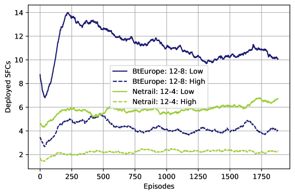
Figure 2: Performance of FIFO

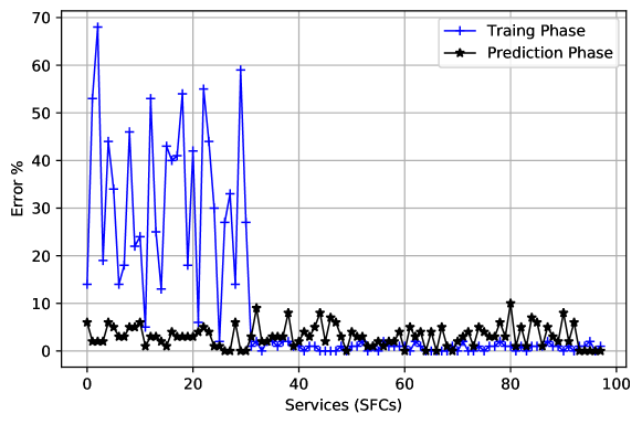
Figure 3: Performance of Online Ridge Regression Model

Figure 3 shows the training phase and Prediction phase of the online-RR model. The model gets trained until its accuracy exceeds 80%, however we only displayed for episode 0 for training phase. Initially, the model observed the SFC till 32 iterations; later, it commenced learning by discovering a logistical approach. Figure 3 depicts the prediction for last episode of a run. It is evident that the model performed well in predicting the priority, as the error% between the predicted and target priority values are less than 10%. Thus, the predicted model’s accuracy was also above 80%.

IV-B Existence of Starvation

The effectiveness of the high-priority-based scheduling paradigm is seen in Fig. 4. Here, the model favours high-priority SFCs above others to avoid the problems caused by FIFO. This triggers a prolonged wait for low-priority SFCs to be deployed, creating a ‘Starvation’ experience and a low acceptance rate. Even with the large nodal resource or higher density topology, as seen in Figure 4, starvation still exists. This starvation gap might slightly get reduced over time for much denser topologies with ample available resources. However, this is unrealistic topology due to the dynamism, where the plentiful resources is not always available.

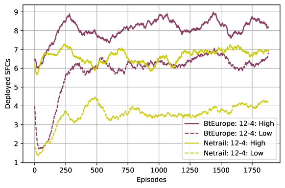
Figure 4: Priority Algorithm Netrail SAR: 12-4 scenario

IV-C Diminish of Starvation

Figure 5 represents the Service Acceptance Rate (SAR) (contains all priority levels, excluding lower-priority SFCs), and Figure 6 depicts the SAR exclusive for low-priority SFCs for Netrail and BtEurope topologies with 12-4 and 12-8 CPU cores. In Figure 5, the WFQ and high-priority-based models embed a large number of high-priority SFCs to establish a deploying rule. This pattern is repeated when topological density or nodal capacity increases. From the figures, the WFQ and high-priority-based models established a deploying rule by embedding only beneficial SFCs. This pattern is repeated when topological density or nodal capacity increases. The DDPG model, on the other hand, discovered a trade-off between high and low-priority SFCs by identifying ‘Beneficial and Starving’ SFCs, resulting in a higher rate of deployment of low-priority SFCs than other models. DDPG, like Netrail 12-4 CPU cores, was able to deploy five times more low-priority SFCs than WFQ at the expense of three less high-priority SFCs. However, in the remaining scenarios (Netrail 12-8; BtEurope 12-4, and BtEurope 12-8), there is a 100% increase in the deployment of low-priority services (Fig.6). This affected high-priority service deployment, with a 30% reduction in Netrail and a 25% reduction in BtEurope (Fig.5) respectively.

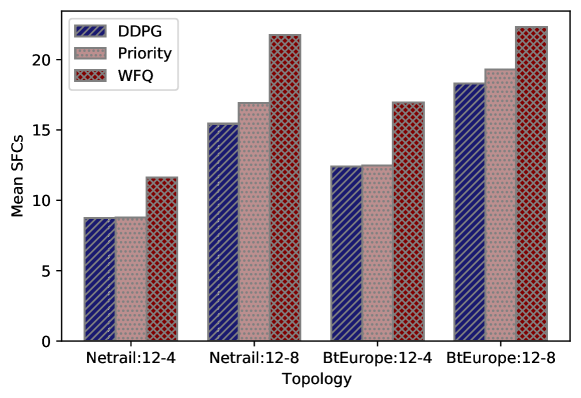
Figure 5: SAR: Deploying Beneficial services

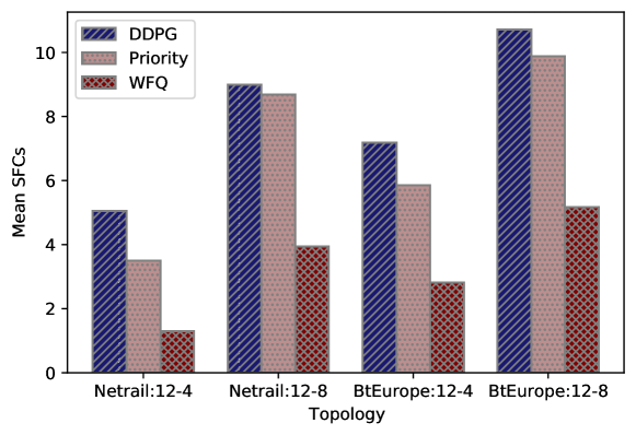
Figure 6: SAR: Deploying Starving services

V Conclusions

The main aim of this study was to showcase the existence of the starvation problem, which the researchers have neglected. In this work, we have explained the existence of the starvation problem in the current scheduling methods and how the scheduling process should not be based only on priority but also on other important factors like threshold waiting time and reliability. With a motive to propose an intelligent scheduling scheme, our model DDPG has performed efficiently by deploying twice as many low-priority services as others. The DDPG agent successfully identified the ‘Beneficial and Starving’ services, which caused a reduction in the starvation of low-priority services. Moreover, we have proposed a method to define dynamic priority for the upcoming services without hindrance. Our online-RR model learns the pattern within 100 transitions, and the accuracy rate for the prediction model is above 80%. The presence of these problems can have a negative impact in the future if not addressed correctly.

5G

the fifth generation of mobile networks

6G

sixth generation of mobile networks

ACO

Ant Colony Optimization

AI

Artificial Intelligence

AR

Augmented Reality

ANN

Artificial Neural Network

AdSch

‘Adaptive Scheduling’

BB

Base Band

BBU

Base Band Unit

BER

Bit Error Rate

BS

Base Station

BW

Bandwidth

BE

Best-Effort

CC

Chain Composition

C-RAN

Cloud Radio Access Networks

CAPEX

Capital Expenditure

CoMP

Coordinated Multipoint

CR

Cognitive Radio

COC

Computation Oriented Communications

CAeC

Contextually Agile eMBB Communications

D2D

Device-to-Device

DA

Digital Avatar

DAC

Digital-to-Analog Converter

DAS

Distributed Antenna Systems

DBA

Dynamic Bandwidth Allocation

DNN

Deep Neural Network

DC

Duty Cycle

DyPr

‘Dynamic Prioritization’

DL

Deep Learning

DSA

Dynamic Spectrum Access

DT

Digital Twin

DRL

Deep Reinforcement Learning

DQL

Deep Q Learning

DDQL

Double Deep Q Learning

DDPG

Deep Deterministic Policy Gradient

$E^{2}D^{2}PG$

Enhanced Exploration Deep Deterministic Policy

ER

Erdős-Rényi

EUB

Expected Upper Bound

EDuRLLC

Event Defined uRLLC

eMBB

enhanced Mobile Broadband

FBMC

Filterbank Multicarrier

FEC

Forward Error Correction

FG

Forwarding Graph

FGE

FG Embedding

FIFO

First-in-First-out

FFR

Fractional Frequency Reuse

FSO

Free Space Optics

GA

Genetic Algorithms

GI

Granularity Index

HAP

High Altitude Platform

HL

Higher Layer

HARQ

Hybrid-Automatic Repeat Request

IoE

Internet of Everything

IoT

Internet of Things

ILP

Integer Linear Program

KPI

Key Performance Indicator

LAN

Local Area Network

LAP

Low Altitude Platform

LL

Lower Layer

LOS

Line of Sight

LTE

Long Term Evolution

LTE-A

Long Term Evolution Advanced

MAC

Medium Access Control

MAP

Medium Altitude Platform

MIMO

Multiple Input Multiple Output

ML

Machine Learning

MME

Mobility Management Entity

mmWave

millimeter Wave

MNO

Mobile Network Operator

MR

Mixed Reality

MILP

Mixed-Integer Linear Program

MDP

Markov Decision Process

mMTC

massive Machine Type Communications

NAI

Network Availability Index

NASA

National Aeronautics and Space Administration

NAT

Network Address Translation

NN

Neural Network

NF

Network Function

NFP

Network Flying Platform

NTN

Non-terrestrial networks

NFV

Network Function Virtualization

NS

Network Service

OFDM

Orthogonal Frequency Division Multiplexing

OSA

Opportunistic Spectrum Access

PAM

Pulse Amplitude Modulation

PAPR

Peak-to-Average Power Ratio

PGW

Packet Gateway

PHY

physical layer

PSO

Particle Swarm Optimization

PT

Physical Twin

PU

Primary User

Pr

Premium

QAM

Quadrature Amplitude Modulation

QoE

Quality of Experience

QoS

Quality of Service

QPSK

Quadrature Phase Shift Keying

QL

Q-Learning

RA

Resource Allocation

RF

Radio Frequency

RN

Remote Node

RRH

Remote Radio Head

RRC

Radio Resource Control

RRU

Remote Radio Unit

RL

Reinforcement Learning

RR

Ridge Regression

SCH

Scheduling

SU

Secondary User

SCBS

Small Cell Base Station

SDN

Software Defined Network

SFC

Service Function Chaining

SLA

Service Level Agreement

SNR

Signal-to-Noise Ratio

SON

Self-organising Network

SAR

Service Acceptance Rate

TDD

Time Division Duplex

TD-LTE

Time Division LTE

TDM

Time Division Multiplexing

TDMA

Time Division Multiple Access

TWT

Threshold Waiting Time

UE

User Equipment

UAV

Unmanned Aerial Vehicle

URLLC

Ultra-Reliable Low Latency Communications

USRP

Universal Software Radio Platform

VL

Virtual Link

VNF

Virtual Network Function

VNF-FG

VNF-Forwarding Graph

VNF-FGE

VNF-FG Embedding

VR

Virtual Reality

WFQ

Weighted Fair Queuing

XAI

Explainable Artificial Intelligence

References

- [1] W. Saad et al., “A Vision of 6G Wireless Systems: Applications, Trends, Technologies, and Open Research Problems,” IEEE netw., 2019.
- [2] H. Ahmadi et al., “Networked Twins and Twins of Networks: An Overview on the Relationship Between Digital Twins and 6G,” IEEE Commun. Stan. Mag., vol. 5, no. 4, pp. 154–160, 2021.
- [3] K. B. Letaief et al., “The roadmap to 6G: AI empowered wireless networks,” IEEE Commun. Mag., vol. 57, no. 8, pp. 84–90, 2019.
- [4] Network functions virtualisation – introductory white paper. [Online]. Available: https://portal.etsi.org/NFV/NFV_White_Paper.pdf
- [5] M. Nekovee et al., “Towards AI-enabled Microservice Architecture for Network Function Virtualization,” in IEEE ComNet, 2020, pp. 1–8.
- [6] S. R. Chowdhury et al., “Re-architecting NFV Ecosystem with Microservices: State of the Art and Research Challenges,” IEEE Netw., vol. 33, no. 3, pp. 168–176, 2019.
- [7] S. B. Chetty et al., “Dynamic decomposition of service function chain using a deep reinforcement learning approach,” IEEE Access, pp. 1–1, 2022.
- [8] P. Cappanera et al., “Vnf placement for service chaining in a distributed cloud environment with multiple stakeholders,” Computer Communications, vol. 133, pp. 24–40, 2019.
- [9] A. Mohamad and H. S. Hassanein, “Psvshare: A priority-based sfc placement with vnf sharing,” in 2020 IEEE Conference on Network Function Virtualization and Software Defined Networks (NFV-SDN). IEEE, 2020, pp. 25–30.
- [10] R. Mijumbi et al., “Design and Evaluation of Algorithms for Mapping and Scheduling of Virtual Network Functions,” in IEEE NetSoft. IEEE, 2015, pp. 1–9.
- [11] S. Agarwal et al., “VNF Placement and Resource Allocation for the Support of Vertical Services in 5G Networks,” IEEE/ACM Trans. on Netw., vol. 27, no. 1, pp. 433–446, 2019.
- [12] Y. Yuan et al., “A Q-learning-based Approach for Virtual Network Embedding in Data Center,” Neural Comput. & Appl., vol. 32, no. 7, pp. 1995–2004, 2020.
- [13] V. Sciancalepore et al., “z-TORCH: An Automated NFV Orchestration and Monitoring Solution,” IEEE Trans. Netw. & Serv. Manag., vol. 15, no. 4, pp. 1292–1306, 2018.
- [14] P. T. A. Quang et al., “A Deep Reinforcement Learning Approach for VNF Forwarding Graph Embedding,” IEEE Trans. Netw. & Serv. Manag., vol. 16, no. 4, pp. 1318–1331, 2019.
- [15] S. B. Chetty et al., “Virtual Network Function Embedding under Nodal Outage using Reinforcement Learning,” in IEEE Intern. Conf. Adv. Netw. & Telec. Sys. IEEE, 2020.
- [16] ——, “Virtual Network Function Embedding under Nodal Outage Using Deep Q-Learning,” Future Internet, vol. 13, no. 3, p. 82, 2021.
- [17] F. Malandrino et al., “Reducing service deployment cost through vnf sharing,” IEEE/ACM Transactions on Networking, vol. 27, no. 6, pp. 2363–2376, 2019.
- [18] M. Jalalitabar et al., “Service function graph design and mapping for nfv with priority dependence,” in 2016 IEEE Global Communications Conference (GLOBECOM). IEEE, 2016, pp. 1–5.
- [19] A. Gupta et al., “On service-chaining strategies using virtual network functions in operator networks,” Comput. Netw., vol. 133, pp. 1–16, 2018.
- [20] A. C. Müller and S. Guido, Introduction to Machine Learning with Python. O’Reilly Media, Inc., 2016.