Position-Guided Point Cloud Panoptic Segmentation Transformer

Abstract

DEtection TRansformer (DETR) started a trend that uses a group of learnable queries for unified visual perception. This work begins by applying this appealing paradigm to LiDAR-based point cloud segmentation and obtains a simple yet effective baseline. Although the naive adaptation obtains fair results, the instance segmentation performance is noticeably inferior to previous works. By diving into the details, we observe that instances in the sparse point clouds are relatively small to the whole scene and often have similar geometry but lack distinctive appearance for segmentation, which are rare in the image domain. Considering instances in 3D are more featured by their positional information, we emphasize their roles during the modeling and design a robust Mixed-parameterized Positional Embedding (MPE) to guide the segmentation process. It is embedded into backbone features and later guides the mask prediction and query update processes iteratively, leading to Position-Aware Segmentation (PA-Seg) and Masked Focal Attention (MFA). All these designs impel the queries to attend to specific regions and identify various instances. The method, named Position-guided Point cloud Panoptic segmentation transFormer (P3Former), outperforms previous state-of-the-art methods by 3.4% and 1.2% PQ on SemanticKITTI and nuScenes benchmark, respectively. The source code and models are available at https://github.com/SmartBot-PJLab/P3Former.

1 Introduction

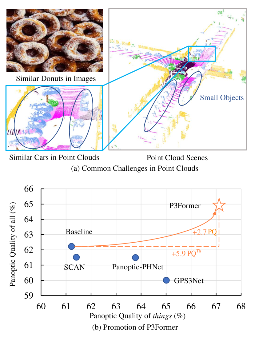
Figure 1: (a) Corner cases in images are common in point cloud scenes: geometrically alike and relatively small objects. (b) Promotion of P3Former with position guidance on SemanticKITTI [2] test set, especially for $\mathrm{PQ}^{\mathrm{Th}}$.

DEtection TRansformer (DETR) [5] started a trend that uses a group of learnable queries for unified visual perception. Various methods, such as K-Net [47] and MaskFormer [9], are proposed to unify and simplify the frameworks of image segmentation. This work begins by applying this appealing paradigm to LiDAR-based point cloud segmentation and obtains a simple yet effective baseline. It relies on transformer decoder and bipartite matching for end-to-end training so that each query can attend to different regions of interest and predict the segmentation mask of either a potential object or a stuff class.

This initial attempt unifies and significantly simplifies the framework for LiDAR-based panoptic segmentation. However, although the naive implementation obtains fair results, the instance segmentation performance is noticeably inferior to previous works (Fig. 1-(b)). Our investigation into this issue reveals two notable challenges in this 3D case: 1) Geometry ambiguity (Fig. 1-(a) left). Instances with similar geometry are much more common in the point clouds than in 2D images and are even harder to be separated due to the lack of texture and colors. 2) Relatively small objects (Fig. 1-(a) right). Instances are typically much smaller with respect to the whole 3D scene, while queries empirically learn to respond to a relatively large area for high recall, making the segmentation of multiple close instances particularly difficult.

Further revisiting the difference between segmentation in images and LiDAR-based point clouds, we observe that instances in images, a dense and structured representation, always have their masks overlapped and their boundaries adhered to each other. In contrast, instances in the 3D space can be clearly separated according to the positional information included in their point clouds. Motivated by this observation, to tackle the aforementioned problems, we fully leverage such properties and propose a Position-guided Point cloud Panoptic Transformer, P3Former, which uses a specialized positional embedding to guide the whole segmentation procedure.

Specifically, we first devise a Mixed-parameterized Positional Embedding (MPE), which combines Polar and Cartesian spaces. MPE incorporates the Polar pattern prior to the point distribution with the Cartesian embedding, resulting in a robust embedding that serves as the foundation of position-guided segmentation. It is first embedded into backbone features as the positional discriminator to separate geometrically alike instances. Furthermore, we also involve it in the mask prediction and masked cross-attention, leading to Position-Aware Segmentation (PA-Seg) and Masked Focal Attention (MFA). PA-Seg introduces a parallel branch for position-based mask prediction alongside the original feature-based one. It compensates for the lack of absolute positional information in high-level features. MFA simplifies the masked attention operation by replacing the cross-attention map with our integrated mask prediction. All these designs enable queries to concentrate on specific positions and predict small masks in a particular region.

We validate the effectiveness of our method on SemanticKITTI [2] and nuScenes [4] panoptic segmentation datasets. P3Former finally performs even better than previous methods on instance segmentation, resulting in new records with a PQ of 64.9% on SemanticKITTI and a PQ of 75.9% on nuScenes, surpassing previous best results by 3.4% and 1.2% PQ, respectively (Fig. 1-(b)). The simplicity and effectiveness of P3Former with our exploration along this pathway shall benefit future research in LiDAR-based panoptic segmentation.

2 Related Work

Figure 2: P3Former  overview. After voxelizing points into voxels, P3Former uses a backbone to extract voxel features and an MPE module to generate the MPE (Sec. 3.2). Apart from being embedded into features, MPE further serves as position guidance in the entire segmentation head. In the segmentation head, we use several PA-Seg (Sec. 3.3) and transformer decoder layers to update queries according to features and MPE, then another PA-Seg layer to predict panoptic results with updated queries. The PA-seg consists of two parallel branches to predict masks from features and MPE, with separate supervision. The integrated masks serve as the cross-attention map in Masked Focal Attention (Sec. 3.4).

Point Cloud Segmentation. Point cloud segmentation aims to map the points into multiple homogeneous groups. Previous works typically resort to different paradigms for indoor [31, 41, 43, 29, 13] and outdoor [35, 36, 20, 33, 19, 1, 49, 10] scenes, given their difference in the point cloud distribution. Our work focuses on the outdoor case, where the point clouds are obtained by LiDAR and exhibit sparse and non-uniform distribution. The corresponding segmentation problem is called LiDAR-based 3D segmentation.

LiDAR-Based 3D semantic segmentation. LiDAR-based 3D semantic segmentation categorizes point clouds according to their semantic properties. Based on different representations of point clouds, we divide existing approaches into three streams, point-based [35, 36, 30], voxel/grid-based [20, 12, 33, 1, 49, 10] and multi-modal [40, 45]. Point-based methods focus on processing individual points, while voxel/grid-based methods quantize point clouds into 3D voxels or 2D grids and apply convolution. Current LiDAR-based segmentation frameworks [49, 10, 40] typically adopt voxel-based backbones due to their ability to capture large-scale spatial structures and acceptable computational cost thanks to sparse convolution [17].

LiDAR-Based 3D panoptic segmentation. Compared with LiDAR-based 3D semantic segmentation, LiDAR-based panoptic segmentation further segments foreground point clouds into different instances. Most previous top-tier works [48, 18, 38, 37, 46, 24] start from this difference and produce panoptic predictions following a three-stage paradigm, i.e., first predict semantic results, then separate instances based on semantic predictions, and finally fuse the two results. This paradigm makes the panoptic segmentation performance inevitably bounded by semantic predictions and requires cumbersome post-processing. In contrast, this paper proposes a unified framework with learnable queries for LiDAR segmentation, eliminating all of these problems and predicting panoptic results unanimously.

Unified Panoptic Segmentation. Unified panoptic segmentation was first proposed in the context of 2D image segmentation. Early works built their methods based on either semantic segmentation frameworks [21, 44, 25, 42] or instance segmentation frameworks [7, 6] to perform panoptic segmentation separately. More recently, DETR [5] simplified the framework for 2D panoptic segmentation, but it still requires two-stage processing.  [47, 9, 8] take this a step further by unifying 2D segmentation in one stage. These methods provide excellent solutions for making queries conditional on specific objects, but they require objects to have distinctive features. As a result, these frameworks may be inferior when dealing with objects that have similar texture and geometry. However, such situations are common in LiDAR-based scenes, resulting in ambiguous instance segmentation.

3 Methodology

This section elaborates on the detailed formation of P3Former (Sec. Fig. 2). We start with a panoptic segmentation baseline that simplifies and unifies the cumbersome frameworks in LiDAR-based panoptic segmentation (Sec. 3.1). To address the challenges hindering this paradigm from performing well in things categories, we propose the Mixed-parameterized Positional Embedding (MPE) to distinguish geometrically alike instances while also fitting the prior distribution of instances (Sec. 3.2). Apart from its conventional usage, the MPE provides robust positional guidance for the entire segmentation process. Specifically, it serves as the low-level positional features, paralleling high-level voxel features in position-aware segmentation(Sec. 3.3). Furthermore, we replace the masked cross-attention map with the combined masks generated from PA-Seg, making the masked attention focus on small instances while also simplifying the attention structure (Sec. 3.4). For more detailed information, please refer to Sec. 3.5.

3.1 Baseline

The baseline mainly consists of two parts: the backbone and the segmentation head. The backbone converts raw points into sparse voxel features, while the segmentation head predicts panoptic segmentation results through learnable queries [47, 9, 8].

Backbone. In this work, we choose Cylinder3D [49] as our backbone for feature extraction due to its good generalization capability for panoptic segmentation [18].

The backbone takes raw points $P\in\mathbb{R}^{\mathrm{N_{P}}\times 4}$ ($x,y,z,r$) as input. Through voxelization and sparse convolution, it outputs sparse voxel features $F\in\mathbb{R}^{\mathrm{V}\times\mathrm{D}}$. Here $\mathrm{N_{P}}$ is the number of points, $r$ is the reflection factor, $\mathrm{V}$ is the number of sparse voxel features, and $\mathrm{D}$ is the feature dimension.

Segmentation Head. We follow the backbone to use voxel representation rather than points as the input to the segmentation head to keep the framework efficient. Vanilla unified segmentation heads consist of two components: One-go Predicting and Query updating. In One-go Predicting, each query predicts one object mask and its category, including things and stuff. The process is as follows:

$$C=f_{C}(Q),\quad M_{F}=f_{MF}(Q)F^{T},$$ (1)

where $f_{C}$ and $f_{MF}$ are different MLP layer.

To make the predictions more adaptive to specific objects, queries need to be updated according to different inputs. Query updating commonly consists of several transformer-based layers. The inputs of layer $l$ are voxel feature $F$, queries $Q_{l-1}\in\mathbb{R}^{\mathrm{N}\times\mathrm{D}}$, and mask predictions $M_{l-1}\in\mathbb{R}^{\mathrm{V}\times\mathrm{N}}$ from layer $l-1$. The outputs are updated query $Q_{l}$. Here $N$ is the query number. Query updating can be formulated as

$$Q_{l}=\mathrm{Updating}(Q_{l-1},M_{l-1},F).$$ (2)

The process can be further decomposed into three parts: Cross-Attention, Self-attention, and Feed-Forward Network (FFN), following the practice of [8]. These can be generally formulated as

$$Q_{Il}=\mathrm{CrossAttn}(Q_{l-1},M_{l-1},F),$$ (3)

and

$$Q_{l}=\mathrm{FFN}(\mathrm{SelfAttn}(Q_{Il}))),$$ (4)

respectively. Here we ignore the expression of the $Add\&Norm$ layer for writing simplicity.

The simple and unified framework can obtain competitive results on stuff categories compared to previous methods. However, the performance on things classes is not ideal due to the special challenges in LiDAR-based scenes.

3.2 Mixed-parameterized Positional Embedding

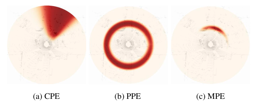
Figure 3: Queries’ positional attention distributions of different positional embedding in Bird-Eye-View.

Distinguishing instances with the same geometry, texture, and colors is one of the biggest challenges for a unified segmentation structure. As shown in Fig.1-(a), separating these donuts is one representative hard task for unified segmentation methods in 2D. Unfortunately, such “donuts” exist nearly everywhere in LiDAR-based scenes: 3D instances don’t have information like texture and color. Meanwhile, they are highly geometrically alike if they belong to the same category, e.g., the ”car” category shown in Fig.1-(b). The main indicator we can utilize is their positional difference.

Positional embedding is a good choice to encode positional information into features. We first formulate positional embedding in Cartesian parameterization, noted as CPE:

$$\mathrm{CPE}=f_{C}([x_{i},y_{i},z_{i}]).$$ (5)

Here $f_{C}$ is a linear transformation layer followed by a normalization layer. It promisingly enhances instances’ discriminability and promotes the performance of the framework. However, this positional embedding parameterization doesn’t offer any distribution prior of LiDAR-based scenes. Consequently, to cover instances as many as possible, each query has learned to attend to a big region (Fig. 3-(a)). While in a crowded scene that contains many relatively small instances, one query would attend to too many instances, which may have negative impacts on the following refinement.

Unlike instances in images that are almost randomly distributed in the picture, instances from LiDAR scans have strong spatial cues (i.e. instances have different distribution patterns depending on distances from the ego vehicle). Learning the distribution prior is helpful for queries to locate small instances in big scenes. Thus, we design a Polar-parameterized positional embedding to help queries fit the distribution, noted as PPE:

$$\mathrm{PPE}=f_{P}([\rho_{i},\theta_{i},z_{i}]),$$ (6)

where $\rho_{i}=\sqrt{x_{i}^{2}+y_{i}^{2}}$, $\theta_{i}=\mathrm{arctan}(y_{i}/x_{i})$, and $f_{P}$ is also a linear transformation layer followed by a normalization layer. It efficiently helps queries to learn ring-shaped attention (Fig. 3-(b)). However, it introduces another problem: instances within the same scan distance are commonly more geometrically alike because of the same point sparsity and scan angle. So they are likely to be segmented as one, although they may not be close in the Cartesian parameterization space.

Based on the observations mentioned above, we propose Mixed Parameterized Positional Embedding (MPE) to leverage the merits of Cartesian and Polar Parameterizations together. Experiments show that simple addition brings ideal promotion above single-format positional embedding. The formulation of MPE is

$$\mathrm{MPE}=f_{P}([\rho_{i},\theta_{i},z_{i}])+f_{C}([x_{i},y_{i},z_{i}]),$$ (7)

We encode MPE into voxel features $F$ and get $F_{P}$:

$$F_{P}=F+MPE,$$ (8)

which replaces $F$ in the above operations.

Fig. 3-(c) demonstrates that MPE maintains ring-like distribution prior while also emphasizing the difference in Cartesian space. Fig. 4-(d) shows that MPE successfully pulls away the distance of instances in the MPE space and makes instances more distinguishable.

Besides, MPE is involved in mask prediction and masked cross-attention, leading to Position-Aware Segmentation (PA-Seg) and Masked Focal Attention (MFA).

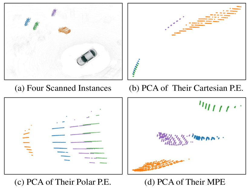
Figure 4: PCA (Principal Component Analysis) of different parameterized positional encoding. Different instances are dyed in origin, green, purple, and blue, respectively. Best viewed in color.

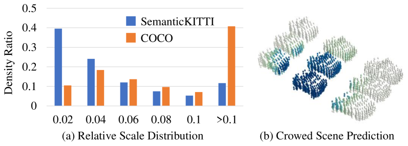
Figure 5: Distribution comparisons of instance relative scale between COCO [27] and SemanticKITTI [2]. Here instance relative scale= $\sqrt{\mathrm{A_{i}}/A_{s}}$ following [14], where $A_{i}$ is the mask area of one instance, $A_{s}$ is the mask area of the whole scene.

3.3 Position-Aware Segmentation

Although the proposed positional embedding strategy can effectively enhance positional information, it is insufficient to deal with small objects, particularly in crowded situations (Fig. 5-(b)), which are also common in LiDAR-based scenes. We count the relative instances scale distribution in Fig. 5-(a). It shows the relative scales of instances in LiDAR-based are much smaller than in images. This observation requires our segmentation head to be more position-aware to discriminate small instances in a crowd.

We rethink the traditional mask prediction (Eq. 1) which only depends on voxel features. Vanilla voxel features generated from the hourglass-like backbone mainly capture high-level geometric information and lack low-level positional information. The embedded MPE partially compensates for the drawback. However, such an operation just uses the MPE implicitly. To this end, we directly predict masks from MPE so queries can explicitly acquire low-level information about a specific position. The formulation is

$$M_{P}=f_{MP}(Q)\cdot\mathrm{MPE},$$ (9)

where $M_{P}$ is position mask and $f_{MP}$ is a MLP layer.

It’s worth noting that we supervise $M_{F}$ and $M_{P}$ separately. We simply use the binary ground truth instance masks $G_{M}$ as the learning targets of $M_{P}$. This is feasible because, in LiDAR-based scenes, instances are concentrated in small local regions and don’t overlap with each other. It shares the same function of center heatmaps used in previous methods, while our solution is more succinct and doesn’t need to generate pseudo centers of instances.

We add $M_{F}$ and $M_{P}$ together to get the final masks $M$, which contain both high-level geometric and low-level positional information. Experiments show that queries with explicit positional awareness will quickly converge to a local region and focus on a small instance.

Table 1: Comparisons of LiDAR panoptic segmentation performance on SemanticKITTI test split. * We don’t use TTA for a fair comparison.

Methods	PQ	$\mathrm{PQ^{{\dagger}}}$	RQ	SQ	$\mathrm{PQ^{Th}}$	$\mathrm{RQ^{Th}}$	$\mathrm{SQ^{Th}}$	$\mathrm{PQ^{St}}$	$\mathrm{RQ^{St}}$	$\mathrm{SQ^{St}}$	FPS
RangeNet++ [33]/PointPillars [23]	37.1	45.9	75.9	47.0	20.2	75.2	25.2	49.3	62.8	76.5	2.4
LPSAD [32]	38.0	47.0	48.2	76.5	25.6	31.8	76.8	47.1	60.1	76.2	11.8
KPConv [41]/PointPillars [23]	44.5	52.5	54.4	80.0	32.7	38.7	81.5	53.1	65.9	79.0	1.9
Panoster [16]	52.7	59.9	64.1	80.7	49.4	58.5	83.3	55.1	68.2	78.8	-
Panoptic-PolarNet [48]	54.1	60.7	65.0	81.4	53.3	60.6	87.2	54.8	68.1	77.2	11.6
DS-Net [18]	55.9	62.5	66.7	82.3	55.1	62.8	87.2	56.5	69.5	78.7	2.1
EfficientLPS [38]	57.4	63.2	68.7	83.0	53.1	60.5	87.8	60.5	74.6	79.5	-
GP-S3Net [37]	60.0	69.0	72.1	82.0	65.0	74.5	86.6	56.4	70.4	78.7	-
SCAN [46]	61.5	67.5	72.1	84.5	61.4	69.3	88.1	61.5	74.1	81.8	12.8
Panoptic-PHNet [24]	61.5	67.9	72.1	84.8	63.8	70.4	90.7	59.9	73.3	80.5	11.0
P3Former	64.9	70.0	75.9	84.9	67.1	74.1	90.6	63.3	77.2	80.7	11.6

Table 2: Comparisons of LiDAR panoptic segmentation performance on nuScenes dataset

Methods	PQ	$\mathrm{PQ^{{\dagger}}}$	RQ	SQ	$\mathrm{PQ^{Th}}$	$\mathrm{RQ^{Th}}$	$\mathrm{SQ^{Th}}$	$\mathrm{PQ^{St}}$	$\mathrm{RQ^{St}}$	$\mathrm{SQ^{St}}$
DS-Net [18]	42.5	51.0	83.6	50.3	32.5	38.3	83.1	59.2	84.4	70.3
EfficientLPS [38]	59.2	62.8	82.9	70.7	51.8	62.7	80.6	71.5	84.1	84.3
GP-S3Net [37]	61.0	67.5	72.0	84.1	56.0	65.2	85.3	66.0	78.7	82.9
SCAN [46]	65.1	68.9	75.3	85.7	60.6	70.2	85.7	72.5	83.8	85.7
Panoptic-PHNet [24]	74.7	77.7	84.2	88.2	74.0	82.5	89.0	75.9	86.9	76.5
P3Former	75.9	78.9	84.7	89.7	76.9	83.3	92.0	75.4	87.1	86.0

3.4 Masked Focal Attention

The integrated mask $M$, which is augmented with position-focusing awareness, can be leveraged as the cross-attention map for query-feature interaction. Vanilla segmentation heads adopt Masked Cross Attention, which is

$$Q_{Il}=\mathrm{softmax}(A_{l-1}+q_{l}k_{l}^{T})v_{l}+Q_{l-1},$$ (10)

where $q_{l}=f_{q}(Q_{l-1})$, $k_{l}=f_{k}(F)$, $v_{l}=f_{v}(F)$. $f_{q}(\cdot),f_{k}(\cdot),f_{v}(\cdot)$ are all linear transformations. The attention mask $A_{l-1}$ at feature location $v\in V$ is

$$A_{l-1}(v)=\left\{\begin{array}[]{rcl}0&&if\ M_{l-1}(v)>0,\\ -\infty&&otherwise.\end{array}\right.$$ (11)

Here the attention map generated by $q_{l}k_{l}^{T}=f_{q}(Q_{l})f_{v}(F)^{T}$ resembles mask prediction $M_{F}$ in Eq. 1 which only uses high-level features $F$. Inspired by Sec. 3.3, we can leverage masks $M$ from position-aware segmentation as the attention map. So Eq. 10 can be reformulated to

$$Q_{Il}=\mathrm{softmax}(A_{l-1}+M)v_{l}+Q_{l-1}.$$ (12)

We refer to it as Masked Focal Attention since the attention features inherit the merit of position-aware masks and focus more on small instances.

3.5 Training and Inference

During training, since the number of predictions $N$ is larger than the pre-defined number of classes, we adopt bipartite matching and set prediction loss to assign ground truth to predictions with the smallest matching cost. For inference, we simply use argmax to determine the final panoptic results.

Loss Functions. Our loss function is composed of a classification loss, a feature-seg loss, and a position-seg loss. We choose focal loss [26] $l_{f}$ for the classification loss $L_{c}$. The feature-seg loss $L_{fs}$ is a weighted summation of binary focal loss $l_{bf}$ and dice loss [39] $l_{df}$. We use dice loss $l_{fp}$ for the position-seg loss $L_{ps}$. The full loss function $L$ can be formulated as $L=L_{c}+L_{fs}+L_{ps}$, while $L_{c}=\lambda_{f}l_{f}$, $L_{fs}=\lambda_{bf}l_{bf}+\lambda_{df}l_{df}$, $L_{ps}=\lambda_{fp}l_{fp}$. In our experiments, we empirically set $\lambda_{f}:\lambda_{bf}:\lambda_{df}:\lambda_{fp}=1:1:2:0.2$.

Hungarian Assignment. Following [5, 9, 47], we adopt the Hungarian assignment strategy to build one-to-one matching between our predictions and ground truth. The formation of matching cost is the same as our loss function.

Inference. Unlike previous LiDAR-based panoptic segmentation methods that need manually designed fusion strategies on semantic and instance segmentation results, we only need to perform argmax among $N$ mask predictions to get the final panoptic results with the dimensions of $1\times\mathrm{V}$.

Iterative Refinement. We stack the Transformer layer several times to refine learnable queries in our framework. During training, we supervise the results predicted by queries before interaction and after each refinement layer with our loss functions. The classification loss is not required for queries before interaction because, at that time, learnable queries are not conditional on specific semantic classes. For inference, we use the results predicted by the finally refined queries.

4 Experiments

In this section, we present the experimental setting and benchmark results on two popular LiDAR-based panoptic segmentation datasets: SemanticKITTI [2] and nuScenes [4]. We also ablate the detailed designs of our proposed methods and provide representative visualizations for qualitative analysis.

4.1 Experimental Setting

SemanticKITTI. SemanticKITTI [2, 3] is the first large-scale dataset on LiDAR-based panoptic segmentation. It contains 43552 frames of outdoor scenes, of which 23201 frames with panoptic labels are used for training and validation, and the remaining 20351 frames without labels are used for testing. The annotations include 8 things classes and 11 stuff classes out of 19 semantic classes.

nuScenes. nuScenes [15] is a public autonomous driving dataset. It provides a total of 1000 scenes, including 850 scenes (34149 frames) for training and validation and 150 scenes (6008 frames) for testing. Among the 16 semantic classes, there are 10 things classes and 6 stuff classes.

Evaluation Metrics. We use the panoptic quality (PQ) [22] as our main metric to evaluate the performance of panoptic segmentation. PQ can be seen as the multiplication of segmentation quality (SQ) and recognition quality (RQ), which is formulated as

$$\small{\text{PQ}}=\underbrace{\frac{\sum_{\mathit{TP}}\text{IoU}}{|\mathit{TP}|}}_{\text{SQ}}\times\underbrace{\frac{|\mathit{TP}|}{|\mathit{TP}|+\frac{1}{2}|\mathit{FP}|+\frac{1}{2}|\mathit{FN}|}}_{\text{RQ}}.$$ (13)

These three metrics can be extended to things and stuff classes, denoted as $\mathrm{PQ^{Th}}$, $\mathrm{PQ^{St}}$, $\mathrm{RQ^{Th}}$, $\mathrm{RQ^{St}}$, $\mathrm{SQ^{Th}}$, $\mathrm{SQ^{St}}$, respectively. We also report PQ^† proposed by [34], which replaces PQ with IoU for stuff classes.

Implementation Details. We implement P3Former with MMDetection3D [11]. We follow Cylinder3D’s [49] procedures for sparse feature extraction and data augmentation on both SemanticKITTI and nuScenes. For sparse feature extraction, we discretize the 3D space to $480\times 360\times 32$ voxels. For data augmentation, we adopt rotation, flip, scale, and noise augmentation. We choose AdamW [28] as the optimizer with a default weight decay of 0.01. In the ablation study, we train the model for 40 epochs with a batch size of 4 on 4 NVIDIA A100 GPUs. The initial learning rate is 0.005 and will decay to 0.001 in epoch 26. More details are provided in the appendix.

4.2 Benchmark Results

SemanticKITTI. We compare our method with RangeNet++ [33] + PointPillars [23], LPSAD [32], KPConv [41] + PointPillars [23], Panoster [16], Panoptic-PolarNet [48], DS-Net [18], EfficientLPS [38], GP-S3Net [37], SCAN [46] and Panoptic-PHNet[24]. Table 1 shows comparisons of LiDAR panoptic segmentation performance on the SemanticKITTI test split. Our method surpasses the best baseline method by 3.4% in terms of PQ. Notably, we outperform the second method  [24] by 3.3% and 3.4% in $\mathrm{PQ^{Th}}$ and $\mathrm{PQ^{St}}$, respectively, suggesting that our unified framework gains in both things and stuff classes.

nuScenes. We also provide the comparison results of LiDAR panoptic segmentation performance on nuScenes validation split. Compared with SemanticKITTI, the point clouds contained in scenes of nuScenes are more sparse, so it can better highlight the model’s ability to model long-distance information. We compare our method with DS-Net [18], EfficientLPS [38], GP-S3Net [37], SCAN [46] and Panoptic-PHNet [24]. As shown in Table 2, our method outperforms existing methods on most of the metrics, surpassing the runner-up method by 1.2% and 2.9% in terms of PQ and $\mathrm{PQ^{Th}}$. It shows that our method has a strong modeling ability for long-distance information and maintains a strong segmentation ability for sparse instances.

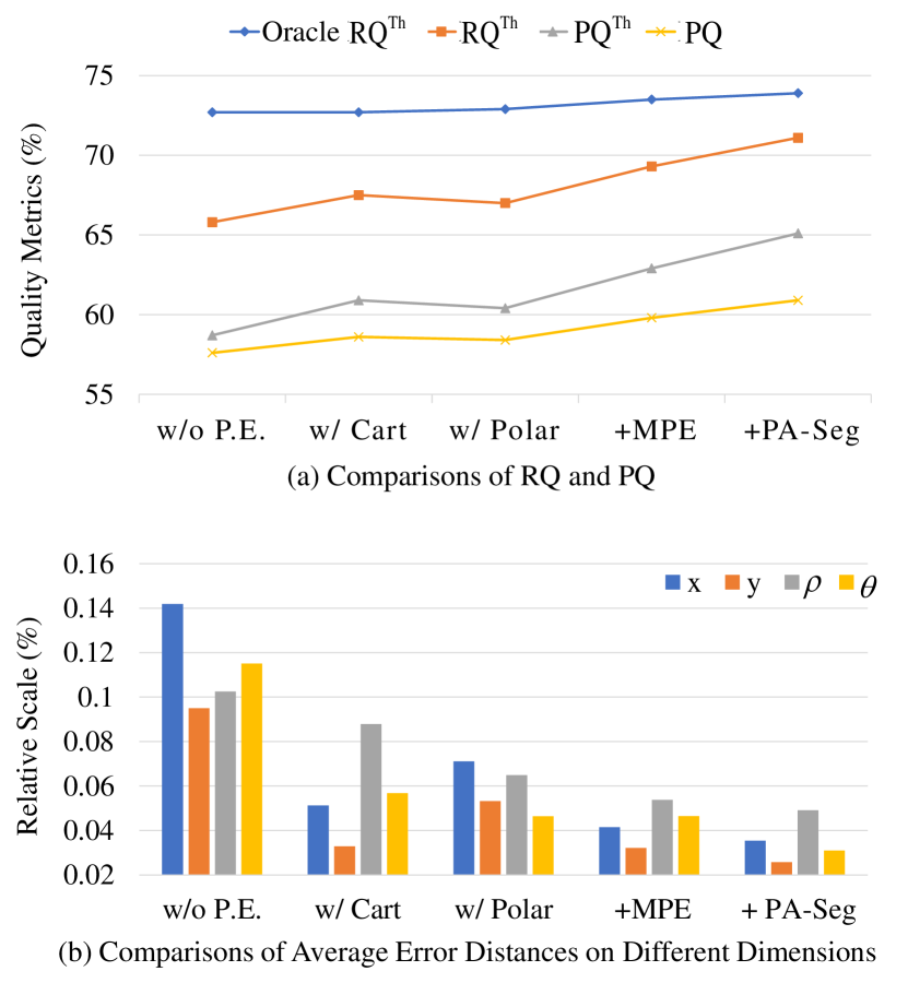
Figure 6: Comparisons of different designs in our model. “Oracle $\mathrm{RQ^{Th}}$” takes all instances included in things prediction as $\mathit{TP}$. “Error distances” measures the one-to-one distances of instances being wrongly predicted as one.

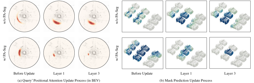
Figure 7: Comparisons of update process with and without PA-Seg. (a) Darker red indicates a high attention level. (b) We construct a crowed scene including 9 similar cars and visualize one query’s mask prediction. Dark blue indicates high prediction confidence.

4.3 Ablation Studies

We conduct several groups of ablations studies in this section to demonstrate the effectiveness of P3Former and detailed information about the framework. All experiments are based on SemanticKITTI [2] validation split.

Effects of Components. We ablate each component that improves the performance of P3Former in Table 3. Our proposed MPE and PA-Seg promote 1.8% PQ (2.8% $\mathrm{PQ^{Th}}$) and 1.1% PQ (2.7% $\mathrm{PQ^{Th}}$) above baseline, respectively. MFA further improve 0.5% PQ and 1.4% $\mathrm{PQ^{Th}}$.

Table 3: Ablation studies of P3Former on SemanticKITTI validation set

Baseline	MPE	PS	MFA	PQ	$\mathrm{PQ^{Th}}$	$\mathrm{PQ^{St}}$
✓				58.0	59.6	57.0
✓	✓			59.8	62.4	57.9
✓	✓	✓		60.9	65.1	57.9
✓	✓	✓	✓	61.4	66.5	57.7

Ambiguous Instance Segmentation. Ambiguous Instance Segmentation (AIS) refers to the case that one query segments multiple instances due to the close feature representation. We conduct a series of experiments to prove that AIS is one of the salient bottlenecks in this task. Specifically, we start from the metric $\mathrm{RQ^{Th}}$ since it is a key component of $\mathrm{PQ^{Th}}$ and a direct indicator of the model’s capability to locate instances. As shown in Fig. 6-(a), there is a huge gap between Oracle $\mathrm{RQ^{Th}}$ and $\mathrm{RQ^{Th}}$ for baseline setting. Since Oracle $\mathrm{RQ^{Th}}$ ignores the AIS cases, it indicates that there are considerable numbers of AIS cases due to the lack of appearance information. Our proposed ingredients effectively remedy the gap, accompanied by the promotion of performance. Here the formulation of Oracle $\mathrm{RQ^{Th}}$ is the same as $\mathrm{RQ^{Th}}$, while we reformulate IoU as Oracle IoU:

$$\text{Oracle IoU}=\frac{P\cap T}{T},$$ (14)

where $P$ indicates prediction areas and $T$ indicates target areas. Oracle IoU measures the percentage of areas that are covered by predictions.

Mixed-parameterized Positional Encoding (MPE). We compare different types of positional encoding in Fig. 6. Fig. 6-(a) shows that Cartesian parameterization (Cart) and Polar parameterization (Polar) are both effective in terms of PQ. The combination of these two can further bring improvements. In Fig. 6-(b) we gather the statistics of the average distances of instances that are wrongly segmented as one on four dimensions $(x,y,\theta,\rho)$. Since instances with smaller distances are harder to separate, methods that achieve smaller average distances on a specific dimension are more accurate on that dimension. It proves that single-parameterized positional encoding can partially improve the model’s accuracy on some dimensions but is deficient on others. A mixed-parameterized one can remedy this drawback.

Table 4: Ablation of Segmentation by Position (SP). “RS” stands for “Relative Scale”, measuring the relative scale of mask predictions.

Metrics	PA-Seg	Layer 0	Layer 1	Layer 3
RS (%)		0.146	0.062	0.036
	✓	0.136	0.045	0.030
PQ (%)		55.8	58.3	59.8
	✓	56.0	59.8	60.9
$\mathrm{PQ^{Th}}$ (%)		54.5	60.1	62.9
	✓	54.6	63.0	65.1

Position-Aware Segmentation (PA-Seg). We validate the effectiveness of PA-Seg in many aspects. Fig. 6-(a) shows that PA-Seg reduces the AIS cases and closes the gap of Oracle $\mathrm{RQ^{Th}}$ and $\mathrm{RQ^{Th}}$. With queries specialize in focused positions, their mask predictions shrink to a more precise area, resulting in smaller relative scale (Table 4) of mask prediction and smaller average error distances (Fig. 6-(b)). PA-Seg leads the queries to quickly be adaptive to their corresponding objects, with larger $\mathrm{PQ}$ and $\mathrm{PQ^{Th}}$ promotion during iterative refinements (Table 4).

4.4 Visual Analysis

Fig 7-(a) illustrates the update process of query positional attention with and without PA-Seg. Queries initially learn positional priors from the dataset and pay attention to a ring-shaped region. During the update, queries without PA-Seg are not aware of updating their positional attention. However, with PA-Seg, queries quickly converge their positional attention and specialize in a small region. Fig. 7-(b) further demonstrates the impact of PA-Seg on mask predictions. The specialization of positional focal attention enabled by PA-Seg aids in successfully separating a car from a crowded scene.

5 Conclusion

We present P3Former for unified LiDAR-based panoptic segmentation. It builds on the DETR paradigm and addresses the challenges of distinguishing small and geometrically similar instances. We introduce a robust Mixed-parameterized Positional Embedding which is embedded into voxel features and further guides the segmentation process, leading to Position-Aware Segmentation and Masked Focal Attention. All these designs enable queries to concentrate on specific positions and predict small masks in a particular region. State-of-the-art performance on SemanticKITTI and nuScenes demonstrate the effectiveness of our framework and reveal the potential of P3Former with more robust 3D representations in future research.

Supplementary Material

Appendix A Implementation Details

For data augmentation, we adopt rotating, flipping, scaling, and noising.

In the voxelization process, we first transform raw point clouds’ Cartesian coordinates ($x,y,z$) into Polar coordinates ($r,\theta,z$). Then we clip the 3D space range into $r\in[0,50],\theta\in[-\pi,\pi],z\in[-4,2]$ for SemanticKITTI [2], and $r\in[0,50],\theta\in[-\pi,\pi],z\in[-5,3]$ for nuScenes [4].

For SemanticKITTI [2] test split results, we use both training split and validation split for training. We train the model for 80 epochs with a batch size of 8 on eight NVIDIA A100 GPUs, as more epochs can continuously optimize the performance. The initial learning rate is 0.005 and will decay to 0.001 in epoch 60.

For inference, we keep mask predictions with sigmoid classification confidences larger than 0.4. After $argmax$, we filter out mask predictions that the IoU of the remaining mask and original mask is smaller than 0.8.

Appendix B Discussions

Model Comparisons. We compare panoptic segmentation models based on the Cylinder3D [49] backbone. As shown in Table 8. We outperform previous methods [49, 18] by a large margin in performance and speed. The comparisons of P3Former with different settings demonstrate that while heavier network settings promote performance, they also add on computational cost and lower the inference speed.

Point vs. Voxel. To implement P3Former, an important choice is the type of 3D representations for segmentation. P3Former uses sparse voxel features rather than points as the input of the segmentation head. Table 5 proves that the voxel type outperforms the point type by 1.5 PQ while about 1.7 times faster in inference. The performance gain of the voxel type is intuitive because, by voxelizing points, we rebalance the varying point density of objects in the scenes.

Table 5: Ablation of Representation Types.

Feature Type	PQ	FPS
Voxel	60.9	19.7
Point	59.4	11.4

Semantic Segmentation. We verify the effectiveness of P3Former on semantic segmentation of SemanticKITTI (Table 6). With interaction mechanism and iterative refinement, we outperform vanilla Cylinder3D decode head by 1.7% mIOU.

Table 6: Results of Semantic Segmentation

Method	mIOU
Cylinder3D	62.5
P3Former	64.2

Loss Weights. Objects are relatively tiny compared with the whole outdoor scene. Thus, the proportion of positive and negative samples in mask supervision is critically imbalanced. From this observation, we select Focal Loss [26] rather than CrossEntropy Loss to alleviate this problem. Besides, we increase the weight of Dice Loss since it can supervise the mask without being influenced by the imbalanced situation. The experimental results are shown in Table 7.

Table 7: Ablation of Loss Weights.

CE	Focal	Dice	PQ	RQ	SQ
1	0	1	58.9	68.9	75.0
0	1	1	59.0	69.2	75.1
0	1	2	59.8	70.8	72.7

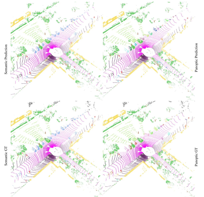
Figure 8: Qualitative examples in SemanticKITTI [3]. Black in GT denotes the ignored class. Instances in panoptic results are randomly colored. Best viewed in color with zoom-in.

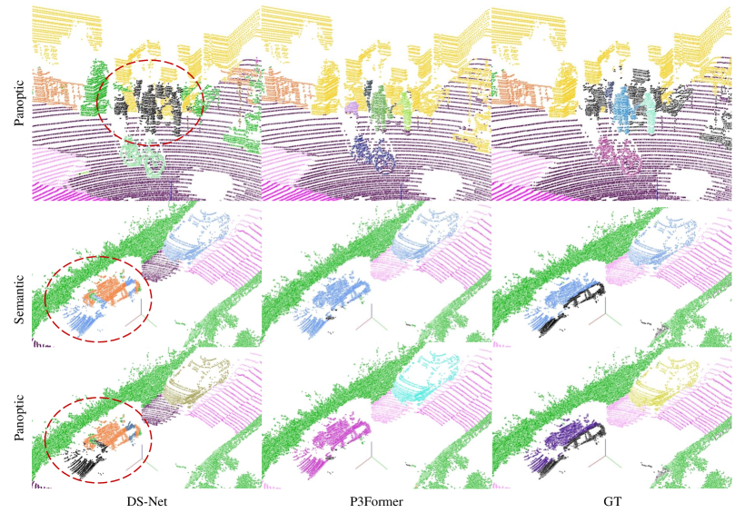
Figure 9: Qualitative comparisons in SemanticKITTI. Black in GT denotes the ignored class. Instances in panoptic results are randomly colored. Best viewed in color with zoom-in.

Appendix C Detailed Benchmarks

We provide class-wise LiDAR panoptic results on SemanticKITTI [2] test set (Table 9), nuScenes [4] dataset (Table 10).

Appendix D Visualizations

Qualitative Comparisons. We show the qualitative examples of semantic and panoptic segmentation on SemanticKITTI [2] in Fig. 8. Our method performs well on large-scale outdoor scenes. Notably, P3Former can effectively handle the situations when instances are truncated because queries separate instances based on not only positional distances but also geometric similarity (Fig. 10-(a, left)). Besides, our approach can tackle the crowded scenarios Fig. 10-(a, right) since queries are specialized in precise positions.

We visualize the predictions of our method and other methods in Fig. 9. Since recent SoTA [37, 46, 24] methods haven’t released their code, we qualitatively compare our method to  [18] (CVPR 2021). The first row of Fig. 9 shows that our methods are better at distinguishing close instances with similar geometry. The second and third rows of Fig. 9 demonstrate that three-stage methods depend a lot on the results of semantic segmentation. If the semantic segmentation fails (the car circled in the second row), the panoptic segmentation is bound to fail. However, with a unified structure like P3Former, we can successfully eliminate this problem.

Failure Cases. However, P3Former still faces some challenges, such as failing to segment some incomplete and close instances (Fig. 10-(b, left)), and wrongly classifying instances due to the highly imbalanced category distribution (Fig. 10-(b, right)). We will investigate these inefficiencies in future studies.

Visualization of Mask Update Processes. We compare the mask update processes between K-Net [47] and P3Former in different domains (Fig. 11). It can be observed that, in images, instances have distinctive appearances, such as colors and textures. Each instance is expected to be assigned to one query before the update. Because instances are likely to overlap with each other, it is critical for queries to be adaptive to instances and refine their boundary during the update.

In contrast, instances in point clouds don’t suffer from overlapping but are commonly geometrically alike. As a result, queries have difficulty separating instances with similar geometric structures and close positions before the update. With our mixed-parameterized positional encoding strategy and position-aware segmentation accentuating positional differences of instances, queries will gradually specialize on specific positions and successfully segment these instances.

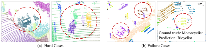
Figure 10: Hard Cases and Failure Cases. (a) P3Former successfully tackles the hard cases of truncated instances (left) and the dense crowd (right). (b) Failure cases of incomplete and close instances (left) and tail categories (right). Best viewed in color with zoom-in.

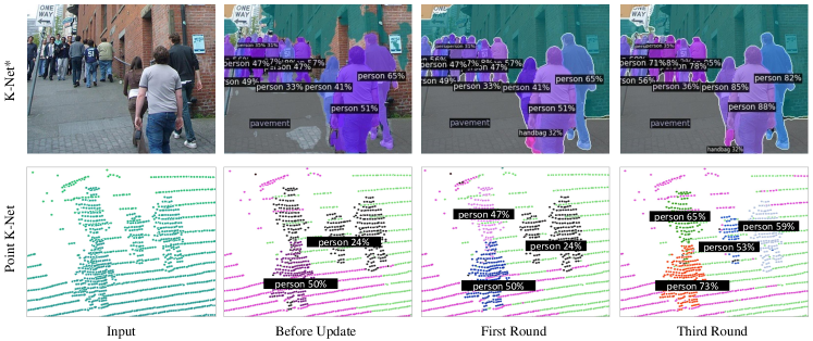
Figure 11: Comparisons of the update processes between K-Net and P3Former. Top line figures are borrowed from K-Net [47]. Best viewed in color with zoom-in.

Table 8: Ablation studies on Model Setting. Here $N_{L}$ indicates iterative layer numbers, $N_{Q}$ indicates the query number and $N_{D}$ indicates the feature dimension. “^†”: We measure the latency with the official codebase released by the authors on our hardware for reference.

Model	$\mathrm{N_{L}}$	$\mathrm{N_{Q}}$	$\mathrm{N_{D}}$	Backbone Size	PQ	RQ	SQ	IoU	Model Size	FPS
Cylinder3D		-		1x	56.4	67.1	76.5	63.5	-	-
DS-Net		-		1x	57.7	68.0	77.6	63.5	221M	$2.1^{{\dagger}}$
P3Former	3	128	128	0.5x	61.4	71.3	75.9	65.5	77M	19.7
	6	128	256	0.5x	62.5	72.4	76.1	66.5	120M	14.2
	6	128	256	1x	62.5	72.3	76.2	66.4	279M	12.5
	6	128	256	1.5x	62.8	72.5	76.4	66.6	559M	11.6

Table 9: Class-wise LiDAR panoptic segmentation results on SemanticKITTI test set

Metrics	Car	Truck	Bicycle	Motorcycle	Other Vehicle	Person	Bicyclist	Motorcyclist	Road	Sidewalk	Parking	Other Ground	Building	Vegetation	Trunk	Terrain	Fence	Pole	Traffic Sign	Mean
PQ	93.0	47.3	52.1	65.6	61.1	75.2	79.4	63.4	89.2	69.4	53.0	19.8	89.4	81.4	63.2	47.7	57.6	58.5	66.7	64.9
RQ	98.5	50.3	68.2	73.3	65.6	84.6	86.1	66.1	96.9	85.6	68.6	26.9	95.0	96.1	82.5	63.5	74.1	77.0	83.3	75.9
SQ	94.4	94.0	76.4	89.5	93.2	89.0	92.2	95.9	92.0	81.1	77.3	73.6	94.1	84.7	76.6	75.0	77.7	75.9	80.1	84.9
mIoU	95.6	49.2	54.8	66.7	57.8	69.9	72.0	38.9	91.5	75.8	67.2	40.1	92.1	86.1	72.4	69.8	68.5	64.0	65.6	68.3

Table 10: Class-wise LiDAR panoptic segmentation results on nuScenes dataset

Metrics	Barrier	Bicycle	Bus	Car	Construction Vehicle	Motorcycle	Pedestrian	Traffic Cone	Trailer	Truck	Driveable Surface	Other Flat	Sidewalk	Terrain	Manmade	Vegetation	Mean
PQ	65.0	68.9	77.1	94.1	61.3	85.2	93.0	91.5	60.2	73.0	96.2	59.6	69.3	57.5	86.9	82.9	75.9
RQ	77.3	79.3	80.3	97.5	67.5	91.5	97.9	97.0	67.5	77.6	99.9	69.3	85.7	73.5	98.3	95.9	84.7
SQ	84.1	86.9	96.0	96.6	90.8	93.1	95.0	94.3	89.3	94.2	96.3	86.0	80.8	78.2	88.4	86.5	89.8
mIoU	68.2	40.3	92.4	93.2	57.0	84.1	76.3	65.1	73.2	85.3	96.5	71.5	74.1	74.8	89.6	87.2	76.8

References

- [1] Inigo Alonso, Luis Riazuelo, Luis Montesano, and Ana C Murillo. 3d-mininet: Learning a 2d representation from point clouds for fast and efficient 3d lidar semantic segmentation. IEEE Robotics and Automation Letters, 5(4):5432–5439, 2020.
- [2] Jens Behley, Martin Garbade, Andres Milioto, Jan Quenzel, Sven Behnke, Cyrill Stachniss, and Jurgen Gall. Semantickitti: A dataset for semantic scene understanding of lidar sequences. In Proceedings of the IEEE/CVF international conference on computer vision, pages 9297–9307, 2019.
- [3] Jens Behley, Andres Milioto, and Cyrill Stachniss. A benchmark for lidar-based panoptic segmentation based on kitti. In 2021 IEEE International Conference on Robotics and Automation (ICRA), pages 13596–13603. IEEE, 2021.
- [4] Holger Caesar, Varun Bankiti, Alex H Lang, Sourabh Vora, Venice Erin Liong, Qiang Xu, Anush Krishnan, Yu Pan, Giancarlo Baldan, and Oscar Beijbom. nuscenes: A multimodal dataset for autonomous driving. In Proceedings of the IEEE/CVF conference on computer vision and pattern recognition, pages 11621–11631, 2020.
- [5] Nicolas Carion, Francisco Massa, Gabriel Synnaeve, Nicolas Usunier, Alexander Kirillov, and Sergey Zagoruyko. End-to-end object detection with transformers. In Computer Vision–ECCV 2020: 16th European Conference, Glasgow, UK, August 23–28, 2020, Proceedings, Part I 16, pages 213–229. Springer, 2020.
- [6] Liang-Chieh Chen, George Papandreou, Iasonas Kokkinos, Kevin Murphy, and Alan L Yuille. Deeplab: Semantic image segmentation with deep convolutional nets, atrous convolution, and fully connected crfs. IEEE transactions on pattern analysis and machine intelligence, 40(4):834–848, 2017.
- [7] Bowen Cheng, Maxwell D Collins, Yukun Zhu, Ting Liu, Thomas S Huang, Hartwig Adam, and Liang-Chieh Chen. Panoptic-deeplab: A simple, strong, and fast baseline for bottom-up panoptic segmentation. In Proceedings of the IEEE/CVF conference on computer vision and pattern recognition, pages 12475–12485, 2020.
- [8] Bowen Cheng, Ishan Misra, Alexander G Schwing, Alexander Kirillov, and Rohit Girdhar. Masked-attention mask transformer for universal image segmentation. In Proceedings of the IEEE/CVF Conference on Computer Vision and Pattern Recognition, pages 1290–1299, 2022.
- [9] Bowen Cheng, Alex Schwing, and Alexander Kirillov. Per-pixel classification is not all you need for semantic segmentation. Advances in Neural Information Processing Systems, 34:17864–17875, 2021.
- [10] Ran Cheng, Ryan Razani, Ehsan Taghavi, Enxu Li, and Bingbing Liu. 2-s3net: Attentive feature fusion with adaptive feature selection for sparse semantic segmentation network. In Proceedings of the IEEE/CVF conference on computer vision and pattern recognition, pages 12547–12556, 2021.
- [11] MMDetection3D Contributors. MMDetection3D: OpenMMLab next-generation platform for general 3D object detection. https://github.com/open-mmlab/mmdetection3d, 2020.
- [12] Tiago Cortinhal, George Tzelepis, and Eren Erdal Aksoy. Salsanext: Fast semantic segmentation of lidar point clouds for autonomous driving. arXiv preprint arXiv:2003.03653, 3(7), 2020.
- [13] Francis Engelmann, Martin Bokeloh, Alireza Fathi, Bastian Leibe, and Matthias Nießner. 3d-mpa: Multi-proposal aggregation for 3d semantic instance segmentation. In Proceedings of the IEEE/CVF conference on computer vision and pattern recognition, pages 9031–9040, 2020.
- [14] Lue Fan, Ziqi Pang, Tianyuan Zhang, Yu-Xiong Wang, Hang Zhao, Feng Wang, Naiyan Wang, and Zhaoxiang Zhang. Embracing single stride 3d object detector with sparse transformer. In Proceedings of the IEEE/CVF Conference on Computer Vision and Pattern Recognition, pages 8458–8468, 2022.
- [15] Whye Kit Fong, Rohit Mohan, Juana Valeria Hurtado, Lubing Zhou, Holger Caesar, Oscar Beijbom, and Abhinav Valada. Panoptic nuscenes: A large-scale benchmark for lidar panoptic segmentation and tracking. IEEE Robotics and Automation Letters, 7(2):3795–3802, 2022.
- [16] Stefano Gasperini, Mohammad-Ali Nikouei Mahani, Alvaro Marcos-Ramiro, Nassir Navab, and Federico Tombari. Panoster: End-to-end panoptic segmentation of lidar point clouds. IEEE Robotics and Automation Letters, 6(2):3216–3223, 2021.
- [17] Benjamin Graham, Martin Engelcke, and Laurens Van Der Maaten. 3d semantic segmentation with submanifold sparse convolutional networks. In Proceedings of the IEEE conference on computer vision and pattern recognition, pages 9224–9232, 2018.
- [18] Fangzhou Hong, Hui Zhou, Xinge Zhu, Hongsheng Li, and Ziwei Liu. Lidar-based panoptic segmentation via dynamic shifting network. In Proceedings of the IEEE/CVF Conference on Computer Vision and Pattern Recognition, pages 13090–13099, 2021.
- [19] Yuenan Hou, Xinge Zhu, Yuexin Ma, Chen Change Loy, and Yikang Li. Point-to-voxel knowledge distillation for lidar semantic segmentation. In Proceedings of the IEEE/CVF Conference on Computer Vision and Pattern Recognition, pages 8479–8488, 2022.
- [20] Qingyong Hu, Bo Yang, Linhai Xie, Stefano Rosa, Yulan Guo, Zhihua Wang, Niki Trigoni, and Andrew Markham. Randla-net: Efficient semantic segmentation of large-scale point clouds. In Proceedings of the IEEE/CVF conference on computer vision and pattern recognition, pages 11108–11117, 2020.
- [21] Alexander Kirillov, Ross Girshick, Kaiming He, and Piotr Dollár. Panoptic feature pyramid networks. In Proceedings of the IEEE/CVF conference on computer vision and pattern recognition, pages 6399–6408, 2019.
- [22] Alexander Kirillov, Kaiming He, Ross Girshick, Carsten Rother, and Piotr Dollár. Panoptic segmentation. In Proceedings of the IEEE/CVF Conference on Computer Vision and Pattern Recognition, pages 9404–9413, 2019.
- [23] Alex H Lang, Sourabh Vora, Holger Caesar, Lubing Zhou, Jiong Yang, and Oscar Beijbom. Pointpillars: Fast encoders for object detection from point clouds. In Proceedings of the IEEE/CVF conference on computer vision and pattern recognition, pages 12697–12705, 2019.
- [24] Jinke Li, Xiao He, Yang Wen, Yuan Gao, Xiaoqiang Cheng, and Dan Zhang. Panoptic-phnet: Towards real-time and high-precision lidar panoptic segmentation via clustering pseudo heatmap. In Proceedings of the IEEE/CVF Conference on Computer Vision and Pattern Recognition, pages 11809–11818, 2022.
- [25] Qizhu Li, Xiaojuan Qi, and Philip HS Torr. Unifying training and inference for panoptic segmentation. In Proceedings of the IEEE/CVF Conference on Computer Vision and Pattern Recognition, pages 13320–13328, 2020.
- [26] Tsung-Yi Lin, Priya Goyal, Ross Girshick, Kaiming He, and Piotr Dollár. Focal loss for dense object detection. In Proceedings of the IEEE international conference on computer vision, pages 2980–2988, 2017.
- [27] Tsung-Yi Lin, Michael Maire, Serge Belongie, James Hays, Pietro Perona, Deva Ramanan, Piotr Dollár, and C Lawrence Zitnick. Microsoft coco: Common objects in context. In Computer Vision–ECCV 2014: 13th European Conference, Zurich, Switzerland, September 6-12, 2014, Proceedings, Part V 13, pages 740–755. Springer, 2014.
- [28] Ilya Loshchilov and Frank Hutter. Decoupled weight decay regularization. arXiv preprint arXiv:1711.05101, 2017.
- [29] Yecheng Lyu, Xinming Huang, and Ziming Zhang. Learning to segment 3d point clouds in 2d image space. In Proceedings of the IEEE/CVF Conference on Computer Vision and Pattern Recognition, pages 12255–12264, 2020.
- [30] Jiageng Mao, Xiaogang Wang, and Hongsheng Li. Interpolated convolutional networks for 3d point cloud understanding. In Proceedings of the IEEE/CVF international conference on computer vision, pages 1578–1587, 2019.
- [31] Hsien-Yu Meng, Lin Gao, Yu-Kun Lai, and Dinesh Manocha. Vv-net: Voxel vae net with group convolutions for point cloud segmentation. In Proceedings of the IEEE/CVF international conference on computer vision, pages 8500–8508, 2019.
- [32] Andres Milioto, Jens Behley, Chris McCool, and Cyrill Stachniss. Lidar panoptic segmentation for autonomous driving. In 2020 IEEE/RSJ International Conference on Intelligent Robots and Systems (IROS), pages 8505–8512. IEEE, 2020.
- [33] Andres Milioto, Ignacio Vizzo, Jens Behley, and Cyrill Stachniss. Rangenet++: Fast and accurate lidar semantic segmentation. In 2019 IEEE/RSJ international conference on intelligent robots and systems (IROS), pages 4213–4220. IEEE, 2019.
- [34] Lorenzo Porzi, Samuel Rota Bulo, Aleksander Colovic, and Peter Kontschieder. Seamless scene segmentation. In Proceedings of the IEEE/CVF Conference on Computer Vision and Pattern Recognition, pages 8277–8286, 2019.
- [35] Charles R Qi, Hao Su, Kaichun Mo, and Leonidas J Guibas. Pointnet: Deep learning on point sets for 3d classification and segmentation. In Proceedings of the IEEE conference on computer vision and pattern recognition, pages 652–660, 2017.
- [36] Charles Ruizhongtai Qi, Li Yi, Hao Su, and Leonidas J Guibas. Pointnet++: Deep hierarchical feature learning on point sets in a metric space. Advances in neural information processing systems, 30, 2017.
- [37] Ryan Razani, Ran Cheng, Enxu Li, Ehsan Taghavi, Yuan Ren, and Liu Bingbing. Gp-s3net: Graph-based panoptic sparse semantic segmentation network. In Proceedings of the IEEE/CVF International Conference on Computer Vision, pages 16076–16085, 2021.
- [38] Kshitij Sirohi, Rohit Mohan, Daniel Büscher, Wolfram Burgard, and Abhinav Valada. Efficientlps: Efficient lidar panoptic segmentation. IEEE Transactions on Robotics, 38(3):1894–1914, 2021.
- [39] Carole H Sudre, Wenqi Li, Tom Vercauteren, Sebastien Ourselin, and M Jorge Cardoso. Generalised dice overlap as a deep learning loss function for highly unbalanced segmentations. In Deep Learning in Medical Image Analysis and Multimodal Learning for Clinical Decision Support: Third International Workshop, DLMIA 2017, and 7th International Workshop, ML-CDS 2017, Held in Conjunction with MICCAI 2017, Québec City, QC, Canada, September 14, Proceedings 3, pages 240–248. Springer, 2017.
- [40] Haotian Tang, Zhijian Liu, Shengyu Zhao, Yujun Lin, Ji Lin, Hanrui Wang, and Song Han. Searching efficient 3d architectures with sparse point-voxel convolution. In Computer Vision–ECCV 2020: 16th European Conference, Glasgow, UK, August 23–28, 2020, Proceedings, Part XXVIII, pages 685–702. Springer, 2020.
- [41] Hugues Thomas, Charles R Qi, Jean-Emmanuel Deschaud, Beatriz Marcotegui, François Goulette, and Leonidas J Guibas. Kpconv: Flexible and deformable convolution for point clouds. In Proceedings of the IEEE/CVF international conference on computer vision, pages 6411–6420, 2019.
- [42] Xinlong Wang, Rufeng Zhang, Tao Kong, Lei Li, and Chunhua Shen. Solov2: Dynamic and fast instance segmentation. Advances in Neural information processing systems, 33:17721–17732, 2020.
- [43] Wenxuan Wu, Zhongang Qi, and Li Fuxin. Pointconv: Deep convolutional networks on 3d point clouds. In Proceedings of the IEEE/CVF Conference on computer vision and pattern recognition, pages 9621–9630, 2019.
- [44] Yuwen Xiong, Renjie Liao, Hengshuang Zhao, Rui Hu, Min Bai, Ersin Yumer, and Raquel Urtasun. Upsnet: A unified panoptic segmentation network. In Proceedings of the IEEE/CVF Conference on Computer Vision and Pattern Recognition, pages 8818–8826, 2019.
- [45] Jianyun Xu, Ruixiang Zhang, Jian Dou, Yushi Zhu, Jie Sun, and Shiliang Pu. Rpvnet: A deep and efficient range-point-voxel fusion network for lidar point cloud segmentation. In Proceedings of the IEEE/CVF International Conference on Computer Vision, pages 16024–16033, 2021.
- [46] Shuangjie Xu, Rui Wan, Maosheng Ye, Xiaoyi Zou, and Tongyi Cao. Sparse cross-scale attention network for efficient lidar panoptic segmentation. In Proceedings of the AAAI Conference on Artificial Intelligence, volume 36, pages 2920–2928, 2022.
- [47] Wenwei Zhang, Jiangmiao Pang, Kai Chen, and Chen Change Loy. K-net: Towards unified image segmentation. Advances in Neural Information Processing Systems, 34:10326–10338, 2021.
- [48] Zixiang Zhou, Yang Zhang, and Hassan Foroosh. Panoptic-polarnet: Proposal-free lidar point cloud panoptic segmentation. In Proceedings of the IEEE/CVF Conference on Computer Vision and Pattern Recognition, pages 13194–13203, 2021.
- [49] Xinge Zhu, Hui Zhou, Tai Wang, Fangzhou Hong, Yuexin Ma, Wei Li, Hongsheng Li, and Dahua Lin. Cylindrical and asymmetrical 3d convolution networks for lidar segmentation. In Proceedings of the IEEE/CVF conference on computer vision and pattern recognition, pages 9939–9948, 2021.