LiteBIRD and CMB-S4 Sensitivities to Reheating in Plateau Models of Inflation

Abstract

We study the sensitivity of LiteBIRD and CMB-S4 to the reheating temperature and the inflaton coupling in three types of plateau-potential models of inflation, namely mutated hilltop inflation, radion gauge inflation, and $\alpha$-attractor T models. We first study the relations between model parameters and CMB observables in all models analytically. We then perform Monte Carlo Markov Chain based forecasts to quantify the information gain on the reheating temperature, the inflaton coupling, and the scale of inflation that can be achieved with LiteBIRD and CMB-S4. We compare the results of the forecasts to those obtained from a recently proposed simple analytic method. We find that both LiteBIRD and CMB-S4 can simultaneously constrain the scale of inflation and the reheating temperature in all three types of models. They can for the first time obtain both an upper and lower bound on the latter, comprising the first ever measurement. In the mutated hilltop inflation and radion gauge inflation models this can be translated into a measurement of the inflaton coupling in parts of the parameter space. Constraining this microphysical parameter will help to understand how these models of inflation may be embedded into a more fundamental theory of particle physics.

1 Introduction

Cosmic inflation [1, 2, 3, 4] continues to be the most popular explanation for the overall homogeneity and isotropy of the observable universe. It can also explain the properties of the small perturbations that are visible in the Cosmic Microwave Background (CMB), and which formed the seeds for galaxy formation. However, very little is known about the mechanism that may have driven the accelerated expansion. A wide range of theoretical models of inflation exist, but the observational data is not sufficient to clearly single out any of them. Moreover, even less is known about how a given model of inflation should be embedded into a more fundamental microphysical theory of nature. Understanding this connection would be highly desirable from the viewpoints of both cosmology and particle physics.

In the next decade the observational situation will change drastically. Upgrades at the South Pole Observatory [5] and the Simmons Observatory [6] aim at pushing the uncertainty in the scalar-to-tensor ratio $r$ down to $\sigma_{r}\sim 3\times 10^{-3}$. In the 2030s JAXA’s LiteBIRD satellite [7] and the ground-based CMB Stage 4 (CMB-S4) program [8] can further reduce this to $\sigma_{r}\sim 1\times 10^{-3}$ and $\sigma_{r}\sim 0.5\times 10^{-3}$. These missions will be sensitive to the impact of reheating on CMB observables [9], caused by the impact of the reheating process on the redshifting of metric perturbations [10, 11, 12]. It has been estimated in [13] that this accuracy should be sufficient to measure the order of magnitude of individual coupling constants in models with a plateau potential, a class of models that is currently favoured by observations. In [14] a simple semi-analytic Bayesian approach was used to confirm this. This calls for a more detailed evaluation of the perspectives to determine the inflaton coupling from CMB data in different models of inflation.

In the present work we investigate the possibility to obtain information on the reheating epoch from future CMB observations through the impact that cosmic reheating has on the redshifting of cosmological perturbations. We focus on three types of models in which inflation is effectively driven by a single scalar field $\Phi$ – namely mutated hilltop inflation (MHI) [15, 16], radion gauge inflation (RGI) model [17, 18] and $\alpha$-attractor T-models ($\alpha$-T) [19, 20, 21] – and assess the capacity of future CMB observations to constrain the scale of inflation, the reheating temperature, and the couplings that connect $\Phi$ to other fields in a model-independent way. Here model-independent means that one can obtain a constraint on the inflaton coupling constants within a given model of inflation without having to specify details of the complete particle physics theory in which this model is embedded. The conditions under which this is possible have been laid out in [13]. We perform Monte Carlo Markov Chain (MCMC) based forecasts using MontePython [22, 23] and compare it to the semi-analytic approach pursued in [14]. In doing so we also include the observational uncertainty in the amplitude of spectral perturbations $A_{s}$, which had been fixed to its best fit value in [14]. In addition to studying $\mathsf{g}$, we also present constraints on the reheating temperature $T_{\rm re}$ in all three models. To the best of our knowledge, these are the first forecasts for the sensitivities of LiteBIRD and CMB-S4 to the reheating $T_{\rm re}$ and $\mathsf{g}$ in these classes of models.

This article is organised as follows. In Sec. 2 we review the general formalism that we use to constrain $T_{\rm re}$ and the inflaton coupling. In Sec. 3 we introduce the three classes of benchmark models that we consider and analytically study the relations between the model parameters and observables. In Sec. 4 we outline two methods for estimating the LiteBIRD and CMB-S4 sensitivities to the reheating temperature and the inflaton coupling. In Sec. 5 we present the results obtained with these methods and discuss them. In Sec. 6 we conclude. In the appendices we comment on the choice of the pivot scale (appendix A), review the conditions under which the inflaton coupling can be constrained from CMB data without having to specify all details of the underlying particle physics models (appendix B), comment on the difficulty to fulfil those conditions in $E$-type $\alpha$-attractor models (appendix C), and present a large set of plots to illustrate the relations between various parameters and observables in the models we consider (appendix D).

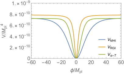
(a)

(b)

Figure 1: The shape of the potential for the mutated hilltop inflation (MHI) model, the radion gauge inflation (RGI) model and the $\alpha$-attractor T ($\alpha$-T) model with their potential given in (35), (39) and (44), and the parameters as used in Sec. 5: in the MHI model $\alpha=3.4$ and $M=5.19\times 10^{-3}M_{pl}$, in the RGI model $\alpha=19$ and $M=5.29\times 10^{-3}M_{pl}$, in the $\alpha$-T model $\alpha=6$ and $M=5.18\times 10^{-3}M_{pl}$. The values of $M$ are chosen according to the fiducial values used in Sec. 5 and summarised in Tab. 2.

2 Review of the formalism

Leaving aside the notable exception of Higgs inflation [25], it is generally believed that inflation was driven by new degrees of freedom beyond the Standard Model (SM) of particle physics. It is clear that these new degrees of freedom must couple to the known particles of the SM in some way (even if only indirectly through a chain of mediators) to enable cosmic reheating [26, 27, 28, 29, 30, 31, 32], i.e., the dissipative transfer of energy from the inflationary sector to other degrees of freedom that filled the universe with particles and set the stage for the hot big bang. Hence, gaining information about reheating would shed light on the connection between inflation and particle physics models beyond the SM. Moreover, reheating is an interesting process on its own because it sets the initial conditions for the radiation dominated epoch. This includes the reheating temperature $T_{\rm re}$, which is an important parameter for the production of thermal relics (such as Dark Matter [33]) and many mechanisms to explain the observed matter-antimatter asymmetry of the universe [34].

The only known direct messenger from the reheating epoch would be gravitational waves (GWs), cf. [35] and references therein. However, it can be studied indirectly through the impact that the post-inflationary expansion history has on the redshifting of CMB perturbations [10, 11, 12]. This has been used to impose constraints on the expansion history of the universe in a wide range of inflationary models, in particular on the duration of the reheating epoch, which are commonly translated into bounds on the reheating temperature $T_{\rm re}$ defined in (13). It has further been pointed out that these constraints can be translated into bounds of microphysical parameters [69] if certain conditions are fulfilled [13]. This possibility has primarily been studied in the context of $\alpha$-attractor models [40, 43, 48, 14]. In the present work we go beyond the existing literature in two ways. Firstly, we for the first time use fully fleshed MCMC forecasts to estimate the sensitivity of LiteBIRD and CMB-S4 to $T_{\rm re}$ in all three classes of models under consideration. Secondly, we use those forecasts to critically assess claims in the previous literature regarding the possibility to constrain microphysical parameters with these experiments.

We focus on scenarios in which the dynamics during inflation and reheating can effectively be described by a single scalar field $\Phi$. We assume that this description holds during both inflation and reheating. and distinguish three types of microphysical parameters.

• A model of inflation is defined by specifying the effective potential $\mathcal{V}(\varphi)$. Ignoring the running couplings during inflation and reheating, specifying $\mathcal{V}(\varphi)$ fixes the set of coefficients $\{\mathsf{v}_{i}\}$ of all operators in the action that can be constructed from $\Phi$ alone. In the models considered here all coefficients $\{\mathsf{v}_{i}\}$ are fixed by two parameters $M$ and $\alpha$.

• The coupling constants (or Wilson coefficients) associated with operators that are constructed from $\Phi$ and other fields form the set of inflaton couplings $\{\mathsf{g}_{i}\}$.

• A complete particle physics model typically contains a much larger number of parameters than the combined sets $\{\mathsf{v}_{i}\}$ and $\{\mathsf{g}_{i}\}$. These include the masses of the particles produced during reheating as well as their interactions amongst each other and with fields other than $\Phi$. We refer to the set of all parameters that are not already contained in $\{\mathsf{v}_{i}\}$ and $\{\mathsf{g}_{i}\}$ as $\{\mathsf{a}_{i}\}$. This set e.g. contains the parameters of the SM.

In the models we consider here there are two free parameters in each potential. One of them indicates the height of the plateaus in Fig. 1. The second one, $\alpha$, characterises the width of the valley in which reheating takes place, and thereby determines the inflaton mass $m_{\phi}$ for fixed $M$. Hence, the two microphysical parameters $M$ and $\alpha$ fix two relevant physical scales, namely the scale of inflation (roughly identified with $M$) and the inflaton mass $m_{\phi}$. The third relevant scale is energy density at the beginning of the radiation dominated epoch, conventionally parameterised in terms of $T_{\rm re}$, which necessarily depends on the inflaton couplings $\{\mathsf{g}_{i}\}$, as they govern the efficiency of the reheating process. We assume that one interaction with coupling constant $\mathsf{g}\in\{\mathsf{g}_{i}\}$ dominates the reheating process. Our goal is then to investigate the constrain the microphysical parameters $\{M,\alpha,\mathsf{g}\}$ that can be obtained with CMB-S4 [8] and LiteBIRD [76]. We restrict ourselves to the observables $\{n_{s},A_{s},r\}$, the relation of which to $T_{\rm re}$ is well-described by the above equations, and which can readily be implemented in forecasts. Here $A_{s}$ is the amplitude of scalar perturbations, $n_{s}$ their spectral index, and $r$ the scalar-to-tensor ratios; the precise definitions of these quantities are given in appendix A.

As discussed in Sec. 3, the ability both of CMB-S4 and LiteBIRD to constrain $\mathsf{g}$ is driven by their sensitivity on the tensor-to-scalar ratio $r$. While Planck’s [86] constraints on $r$ come from the large scales of the CMB temperature anisotropy spectrum, the sensitivity on $r$ of CMB-S4 and LiteBIRD (and BICEP [87]) comes from measuring the B-mode polarization spectrum of the CMB. The primordial B mode spectrum (generated by tensor perturbations) gets contaminated by CMB lensing which converts E-modes (generated by scalar perturbations) into B-modes. This brings out two observable windows for B-modes, namely the reionization bump at the largest scales, $\ell\lesssim 10$, and the recombination bump centered at $\ell\approx 80$. At smaller scales, $\ell\gtrsim 100$, the primordial tensor modes are already sub-horizon during recombination implying the B modes to quickly drop off while the lensing contaminant becomes entirely dominant. Even though both experiments – CMB-S4 and LiteBIRD – have as one of their main science goals the measurement of primordial B-modes, they are considered being complimentary as they aim to measure them on different scales. LiteBIRD targets to measure the reionization bump at the very large scales where the lensing contamination is expected to be very small. The satellite mission is therefore designed with very good sensitivity but modest resolution. CMB-S4 in contrast aims to measure the recombination bump which requires removal of the lensing induced B modes. This is aimed to be done via a procedure called delensing: The lensing induced B-mode signal is predicted from the measurements of the lensing potential and the E-mode spectrum and then subtracted from the measured B-modes, the remains should be the primordial ones. CMB-S4 will consist of many ground-based detectors providing very good sensitivity and resolution (required for successful delensing) but only small sky coverage.

2.1 General formalism

We assume that the time evolution of the field expectation value $\varphi\equiv\langle\Phi\rangle$ follows an equation of motion of the form

$$\ddot{\varphi}+(3H+\Gamma)\dot{\varphi}+\partial_{\varphi}\mathcal{V}(\varphi)=0.$$ (1)

Here $\mathcal{V}(\varphi)$ is an effective potential, $\Gamma$ an effective damping rate for $\varphi$, $H=\dot{a}/a$ the Hubble rate, with $a$ the scale factor. Inflation ends when the equation of state exceeds $w>-1/3$, i.e., the universe stops accelerating. For practical convenience we here define the end of inflation (and thus the beginning of reheating) in terms of the slow roll parameters

$$\epsilon=\frac{M^{2}_{pl}}{2}\left(\frac{\partial_{\varphi}\mathcal{V}}{\mathcal{V}}\right)^{2}\ ,\quad\eta=M^{2}_{pl}\frac{\partial^{2}_{\varphi}\mathcal{V}}{\mathcal{V}},$$ (2)

by the field value $\varphi_{\rm end}$ with $\epsilon|_{\varphi_{\rm end}}=1$. The reheating epoch ends when the energy density of radiation $\rho_{R}$ exceeds the energy density $\rho_{\varphi}\simeq\dot{\varphi}^{2}/2+\mathcal{V}$ of the condensate $\varphi$ and the universe becomes radiation dominated ($w=1/3$). This moment in good approximation coincides with the moment when $\Gamma=H$, and we in the following use the latter equality to define the end of reheating.

For a given model of inflation the power spectrum of cosmological perturbations at the end of inflation is fixed in terms of the parameters $\{\mathsf{v}_{i}\}$ in the potential $\mathcal{V}(\varphi)$. The impact that the reheating epoch has on the redshifting of these perturbations is primarily sensitive to the duration of the reheating epoch in terms of $e$-folds $N_{\rm re}$ and the averaged equation of state $\bar{w}_{\rm re}$ during reheating,

$$\bar{w}_{\rm re}=\frac{1}{N_{\rm re}}\int_{0}^{N_{\rm re}}w(N)dN.$$ (3)

The latter is in good approximation fixed by the $\{\mathsf{v}_{i}\}$, as the inflaton condensate $\varphi$ dominates the energy density and pressure during reheating (and hence $\bar{w}_{\rm re}$). Hence, $N_{\rm re}$ is the only parameter that cannot be fixed by specifying the potential $\mathcal{V}(\varphi)$ (i.e., the parameters $\{\mathsf{v}_{i}\}$).

We follow the approach taken in section 2.2 of ref. [43], which is based on the derivation given in [40]. $N_{\rm re}$ can be expressed as

$$N_{\rm re}=\frac{4}{3\bar{w}_{\rm re}-1}\left[N_{k}+{\rm ln}\left(\frac{k}{a_{0}T_{0}}\right)+\frac{1}{4}{\rm ln}\left(\frac{40}{\pi^{2}g_{*}}\right)+\frac{1}{3}{\rm ln}\left(\frac{11g_{s*}}{43}\right)-\frac{1}{2}{\rm ln}\left(\frac{\pi^{2}M^{2}_{pl}rA_{s}}{2\sqrt{\mathcal{V}_{\rm end}}}\right)\right]~{},$$ (4)

where $M_{pl}=2.435\times 10^{18}~{}{\rm GeV}$ is the reduced Planck mass, and $g_{*}$ and $g_{s*}$ are the effective number of degrees of freedom contributing to the energy- and entropy-densities of the plasma, respectively. We use $g_{*}=g_{s*}=10^{2}$ in this work. $N_{k}$ is the e-folding number between the horizon crossing of a perturbation with wave number $k$ and the end of inflation,

$$N_{k}={\rm ln}\left(\frac{a_{\rm end}}{a_{k}}\right)=\int_{\varphi_{k}}^{\varphi_{\rm end}}\frac{Hd\varphi}{\dot{\varphi}}\approx\frac{1}{M^{2}_{pl}}\int_{\varphi_{\rm end}}^{\varphi_{k}}d\varphi\frac{\mathcal{V}}{\partial_{\varphi}\mathcal{V}}~{},$$ (5)

with $a_{0}$ being the scale factor at present time and $T_{0}=2.725~{}{\rm K}$ the temperature of the CMB at the present time. We introduce the subscript notation $H_{k},\varphi_{k},\epsilon_{k},\eta_{k}$ to indicate the value of the respective quantities $H,\varphi,\epsilon,\eta$ in the moment when the mode $k$ crosses the horizon. In this work we pick $k_{p}/a_{0}=0.05{\rm Mpc}^{-1}$ as this pivot scale of the CMB data. In the past, sometimes the pivot scale $k/a_{0}=0.002{\rm Mpc}^{-1}$ has been used to determine the scalar-to-tensor ratio, which we will denote by $r_{0.002}$. We comment on the relation between $r$ and $r_{0.002}$ in appendix A. $\varphi_{k}$ can be expressed in terms of the CMB parameters, namely the spectral index $n_{s}$ and the tensor-to-scalar ratio $r$, through the relation

$$n_{s}=1-6\epsilon_{k}+2\eta_{k}~{},\quad r=16\epsilon_{k}~{},$$ (6)

From the slow roll approximation, we obtain

$$H^{2}_{k}=\frac{\mathcal{V}(\varphi_{k})}{3M_{pl}^{2}}~{}=\pi^{2}M_{pl}^{2}\frac{rA_{s}}{2}.$$ (7)

In the present work we consider three observables $\{n_{s},A_{s},r\}$. From (6) we obtain

$$\epsilon_{k}=\frac{r}{16}~{},\quad\eta_{k}=\frac{n_{s}-1+3r/8}{2}.$$ (8)

Combining this with (2) we find

$$\frac{\partial_{\varphi}\mathcal{V}(\varphi)}{\mathcal{V}(\varphi)}\Bigl{|}_{\varphi_{k}}=\sqrt{\frac{r}{8M_{pl}^{2}}}\ ,\quad\frac{\partial^{2}_{\varphi}\mathcal{V}(\varphi)}{\mathcal{V}(\varphi)}\Bigl{|}_{\varphi_{k}}=\frac{n_{s}-1+3r/8}{2M_{pl}^{2}}.$$ (9)

Together with (7) this provides three equations that relate the effective potential and its derivatives to the three observables $\{n_{s},A_{s},r\}$. The overall normalisation $M$ of $\mathcal{V}(\varphi)$ has to be obtained from (7), then the two equations in (9) permit to identify one more parameter in the potential (which is typically necessary to determine the inflaton mass) and $N_{\rm re}$. This at least in principle permits to determine three microphysical parameters from observation, which we typically choose as the overall normalisation of the potential $M$, the inflaton coupling $\mathsf{g}$, and one more parameter $\alpha$ in the potential that determines the inflaton mass $m_{\phi}$. For the models considered in this work the solution for the set of equations relating $\{M,\alpha,\mathsf{g}\}$ is always invertible within the observationally allowed range for $\{n_{s},A_{s},r\}$. However, the current error bar on $n_{s}$ is too large to fit all three parameters, cf. e.g. Fig. 4.

2.2 Constraining the reheating temperature

Knowledge of $N_{\rm re}$ and $w_{\rm re}$ permits to compute the energy density $\rho_{\rm re}$ at the end of reheating

$$\rho_{\rm re}=\rho_{\rm end}\exp(-3N_{\rm re}(1+\bar{w}_{\rm re})),$$ (10)

by using the redshifting relation $\rho(N)=\rho_{\rm end}\exp[-3\int_{0}^{N}(1+w(N^{\prime}))dN^{\prime}]$ to write the Friedmann equation as

$$H^{2}=\frac{\rho_{\rm end}}{3M^{2}_{pl}}e^{-3N_{\rm re}(1+\bar{w}_{\rm re})}.$$ (11)

The energy density at the end of inflation $\rho_{\rm end}$ is also determined by the parameters of the inflationary model

$$\rho_{\rm end}\simeq\frac{4}{3}\mathcal{V}_{\rm end}$$ (12)

where $\mathcal{V}_{\rm end}$ is the potential at the end of inflation. The energy density $\rho_{\rm re}$ is often expressed in terms of an effective reheating temperature defined by the relation

$$\frac{\pi^{2}g_{*}}{30}T_{\rm re}^{4}\equiv\rho_{\rm re}.$$ (13)

$T_{\rm re}$ can be identified with a physical temperature in the thermodynamic sense if the decay products reach local thermal equilibrium quickly, cf. refs. [88, 89, 90, 91] for a discussion, otherwise it should be interpreted as an effective parameter that parameterises the energy density $\rho_{\rm re}$. Assuming that reheating happens instantaneously when $\Gamma=H$, one obtains the standard relation

$$T_{\rm re}=\sqrt{\Gamma M_{pl}}\left(\frac{90}{\pi^{2}g_{*}}\right)^{1/4}\Big{|}_{\Gamma=H}..$$ (14)

Solving (13) and (10) for $T_{\rm re}$ gives

$$T_{\rm re}=\exp\left[-\frac{3(1+\bar{w}_{\rm re})}{4}N_{\rm re}\right]\left(\frac{40\mathcal{V}_{\rm end}}{g_{*}\pi^{2}}\right)^{1/4}.$$ (15)

Leaving aside the mild dependence on $g_{*}$, $N_{\rm re}$ is the only parameter on the RHS of (15) that is not determined by fixing the parameters $\{\mathsf{v}_{i}\}$ in $\mathcal{V}$. Hence, determining $T_{\rm re}$ boils down to establishing a relation between $N_{\rm re}$ and observable quantities by plugging (4) with (5) into (15), where $\varphi_{k}$ is determined by solving (6), and $\mathcal{V}_{\rm end}$ and $\varphi_{\rm end}$ are obtained by solving $\epsilon=1$ for $\varphi$. This opens up the possibility to constrain the reheating temperature from observation.

Before moving on, we recall that $T_{\rm re}$ is already constrained by the good agreement between theoretical calculations of big bang nucleosynthesis (BBN) and the abundances of light elements in the intergalactic medium [92], imposing a lower bound

$$T_{\rm re}>T_{\rm BBN}.$$ (16)

The highest temperature that directly affects BBN is the freeze-out of neutrinos, which happens at roughly $1.4$ MeV (cf. e.g. [93]). However, since different modes freeze out at different temperatures, the lower bound on the reheating temperature is in fact a bit higher (cf. e.g. [94]). In the present work we use $T_{\rm BBN}=10$ MeV.

2.3 Constraining the inflaton coupling

Any information about $T_{\rm re}$ discussed in the previous section 2.2 is already of great interest from the viewpoint of particle physics because the thermal history of the universe determines the abundances of thermal relics and is crucial for the viability of baryogenesis scenarios. We go one step further and establish a more direct connection between CMB observables and fundamental interactions by converting the information on $N_{\rm re}$ into constraints on microphysical parameters, in particular the inflaton coupling $\mathsf{g}$. This is possible because $N_{\rm re}$ is primarily determined by the efficiency of the energy transfer from $\varphi$ to radiation, which we characterise by an effective dissipation rate $\Gamma$. This transfer at a microscopic level is driven by fundamental interactions between elementary particles. Hence, $N_{\rm re}$ is in principle sensitive to the fundamental parameters that govern these interactions.

interaction	$y\Phi\bar{\psi}\psi$	$g\Phi\chi^{2}$	$\frac{\sigma}{\Lambda}\Phi F_{\mu\nu}\tilde{F}^{\mu\nu}$	$\frac{h}{3!}\Phi\chi^{3}$
$\mathsf{g}$	$y$	$\tilde{g}=g/m_{\phi}$	$\tilde{\sigma}=\sigma m_{\phi}/\Lambda$	$h$
$\#$	$8\pi$	$8\pi$	$4\pi$	$3!64(2\pi)^{3}$
rescaling factor	$1$	1	$\frac{1}{\sqrt{2}}$	$8\sqrt{6}\pi$

Table 1: Conversion of the bounds on the Yukawa coupling $y$ into bounds on the other couplings in (19). Note that the simple conversion by multiplying with a number is only possible when $\Gamma$ is expressed in the form (18). In particular, it does not apply to the dimensionful couplings $g_{\phi}$, $g$ and $\sigma$, but only to the dimensionless ratios (21).

We can use the Friedmann equation (11) and the knowledge that reheating ends when $\Gamma=H$ to obtain the identity

$$\Gamma|_{\Gamma=H}=\frac{1}{M_{pl}}\left(\frac{\rho_{\rm end}}{3}\right)^{1/2}e^{-3(1+\bar{w}_{\rm re})N_{\rm re}/2}.$$ (17)

Within a given model of inflation all parameter on the RHS of (17) can be expressed in terms of CMB observables $\{n_{s},A_{s},r\}$ by applying the procedure sketched in Sec. 2.1, while the LHS is in principle calculable in terms of microphysical parameters when the inflaton interactions are specified. $\Gamma$ necessarily depends on the $\{\mathsf{g}_{i}\}$ and $\{\mathsf{v}_{i}\}$. For instance, for reheating through elementary particle decays, one typically finds

$$\Gamma=\mathsf{g}^{2}m_{\phi}/{\#},$$ (18)

with $\mathsf{g}\in\{\mathsf{g}_{i}\}$ a coupling constant, $m_{\phi}\in\{\mathsf{v}_{i}\}$ the inflaton mass, and $\#$ a numerical factor. A set of explicit examples for interactions that lead to decay rates of this form are given in table 1 They include interactions of $\Phi$ with other scalars $\chi$, fermions $\psi$ with gauge interactions as well as U(1) gauge bosons with field strength tensor $F_{\mu\nu}$. In this work we consider the operators

$$g\Phi\chi^{2}\ ,\quad\frac{\sigma}{\Lambda}\Phi F_{\mu\nu}\tilde{F}^{\mu\nu}\ ,\quad y\Phi\bar{\psi}\psi,\quad\frac{h}{3!}\Phi\chi^{3}$$ (19)

The interactions (19) yield $\Gamma$ of the form (18), cf. table 1. If the effective dissipation rate $\Gamma$ at the moment when it equals the Hubble rate $H$ is dominated by elementary decays, one can plug (18) into (17) and solve for $\mathsf{g}$ to translate a constraint on $N_{\rm re}$ into one on $\mathsf{g}$. This dependence has been explored in $\alpha$-attractor models in [40, 43, 48, 14]. In general this procedure is hampered by the fact that feedback effects invalidate the usage of (18) in (17) and introduce a dependence on the $\{\mathsf{a}_{i}\}$, making a determination of $\mathsf{g}$ from CMB data impossible. The conditions on the $\{\mathsf{v}_{i}\}$ and $\mathsf{g}$ under which these effects can be avoided have been studied in [13] and are briefly sketched in appendix B.

When it comes to the self-interactions we restrict ourselves to values of the parameters $\{\mathsf{v}_{i}\}$ in $\mathcal{V}(\varphi)$ for which these conditions are fulfilled, as otherwise no model-independent constraint on any microphysical parameter can be derived, irrespective of the value of $\mathsf{g}$. To identify the parameter range where this is guaranteed we expand

$$\mathcal{V}(\varphi) = \frac{1}{2}m_{\phi}^{2}\varphi^{2}+\frac{g_{\phi}}{3!}\varphi^{3}+\frac{\lambda_{\phi}}{4!}\varphi^{4}+\mathcal{O}[\varphi^{5}],$$ (20)

with $\mathsf{v}_{3}=g_{\phi}/3!$ and $\mathsf{v}_{4}=\lambda_{\phi}/4!$. It is convenient to introduce the dimensionless coupling constants,

$$\tilde{g}\equiv\frac{g}{m_{\phi}}\quad,\quad\tilde{\sigma}\equiv\frac{m_{\phi}}{\Lambda}\sigma\quad,\quad\tilde{g}_{\phi}\equiv\frac{g_{\phi}}{m_{\phi}}$$ (21)

so that $\mathsf{g}\in\{\tilde{g},\tilde{\sigma},y,h\}$ and $\mathsf{v}_{i}\in\{\tilde{g}_{\phi},\lambda_{\phi}\}$. The conditions under which (18) can be used on the LHS of (17) read [13]

(24)

The conditions in (24) practically restrict us to symmetric potentials and field oscillations that are approximately harmonic with a frequency given by the inflaton mass $m_{\phi}$, so that

$$\bar{w}_{\rm re}=0.$$ (25)

A very simple criterion on the potential can be imposed by demanding that the cubic and quartic terms are sub-dominant at the end of inflation, i.e.,

$$\varphi_{\rm end}<\varphi_{\rm cr},\tilde{\varphi}_{\rm cr}\quad{\rm with}\quad\varphi_{\rm cr}^{2}=\frac{12}{\lambda_{\phi}}m_{\phi}^{2}\ ,\ \tilde{\varphi}_{\rm cr}=\frac{3m_{\phi}^{2}}{g_{\phi}}.$$ (26)

Note that the simple criterion (26) represents a necessary, but not a sufficient condition, and that (24) in general is more constraining.

When it comes to the inflaton coupling to other fields $\mathsf{g}$, we ignore the restrictions arising from the requirement to justify usage of (18) on the LHS of (17) in the forecasts, but indicate the region where it is not fulfilled. In plateau-type inflation models these restrictions can parametrically be estimated by

$$|\mathsf{v}_{j}|\ll\left(3\pi^{2}rA_{s}\right)^{(j-2)/2}\ ,\ |\mathsf{g}|\ll\left(3\pi^{2}rA_{s}\right)^{j/2},$$ (27)

with $j$ the power at which $\Phi$ appears in a given interaction term, and we have ignored various numerical factors. While (27) provides a simple criterion that can easily be compared with observational constraints, it relies on additional assumptions compared to the criteria introduced in [13], cf.  appendix B. In our analysis we use the mode general condition (68) given in that appendix. These conditions impose a very strong constraint on couplings with $j>1$. Luckily they are too conservative in many realistic scenarios. We briefly comment on this in Appendix B. Note also that (68) only restricts the translation of a bound on $N_{\rm re}$ into a constraint on $\mathsf{g}$ via (17). Imposing a bound on $\rho_{\rm re}$ or $T_{\rm re}$ via (15) is still perfectly possible in the regime where these conditions are violated.

2.4 Basic Example: Chaotic inflation

Figure 2: Impact of the reheating phase on the predictions of the model (28) for $n_{s}$ and $r$. The relation (29) fixes a line in the ($n_{s}$, $r$) plane. Along this line each point corresponds to a specific choice of values for $\mathsf{g}$ and $T_{\rm re}$. The dependence is monotonic, larger values of $\mathsf{g}$ (and hence $T_{\rm re}$) correspond to smaller values of $r$ and larger values of $n_{s}$. Here we identify $\mathsf{g}$ with the Yukawa coupling $y$ in table 1. The predictions for ${\rm log}_{10}y$ are given by the numbers above the discs. The value ${\rm log}_{10}y=-17$ (red disc) corresponds to $T_{\rm re}=T_{\rm BBN}$, smaller values are ruled out by the condition (53). The yellow disc with ${\rm log}_{10}y=-12.8$ marks the point to the right of which $T_{\rm re}$ exceed the temperature of the electroweak sphaleron freezeout $T_{\rm sph}\simeq 131$ GeV, cf. footnote 12. The green disc indicates the point where $N_{k}=50$. The red and blue areas display marginalized joint confidence regions for $(n_{s},r)$ at the $1\sigma$ $(68\%)$ CL (dark) and $2\sigma$ $(95\%)$ CL (light) from Planck+BICEP/Keck 2015 and 2018 data, respectively (Fig. 28 in [86] and Fig. 5 in [87], respectively).

The present work is dedicated to plateau-type models of inflation, which are currently favoured by observational data. Before moving to the discussion of realistic models of this type we start with a brief discussion of the potential

$$\mathcal{V}(\varphi)=\frac{1}{2}m_{\phi}^{2}\varphi^{2},$$ (28)

the simplest example of a monomial potential [99], which can also act as an effective description of string-inspired scenarios [100, 101]. The effect of reheating in the model (28) has previously been studied in [102]. Though it is by now severely disfavoured by the observational upper bound on $r$, cf. Fig. 2, its simplicity makes it suitable for illustrative purposes. For the potential (28) one finds $\epsilon=\eta=2M_{pl}^{2}/\varphi^{2}$, which leads to

$$1-n_{s}=\frac{r}{4}.$$ (29)

Solving $\epsilon|_{\varphi=\varphi_{\rm end}}=1$ in (2) and $r=16\epsilon_{k}$ in (6) respectively we find

$$\varphi_{\rm end}=\sqrt{2}M_{pl},\quad\varphi_{k}=4\sqrt{\frac{2}{r}}M_{pl}~{}.$$ (30)

Inserting them into (5) we get a simple expression for $N_{k}$,

$$N_{k}=\frac{8}{r}-\frac{1}{2}~{}.$$ (31)

Note that the above relations are entirely independent of $m_{\phi}$ and also independent of $\mathsf{g}$. The fact that specifying the potential defines a line in the $n_{s}$-$r$-plane is a general result that applies to all models under consideration here. The shape of this line is typically independent of $\mathsf{g}$. Fixing $\mathsf{g}$ then determines where on the line the model prediction lies, cf. Fig. 2. However, the fact that the position of the line defined by (29) is independent the only parameter $m_{\phi}$ in the potential (28) is a particularity of this simple model. In general, choosing a type of potential defines a family or curves in the $n_{s}$-$r$-plane, and selecting a specific curve within this family requires fixing some parameters in the potential.

Fixing $m_{\phi}$ by (7) requires knowledge of $A_{s}$ (but does not explicitly depend on $n_{s}$),

$$m_{\phi}=\sqrt{\frac{3}{32}}\pi\ \sqrt{A_{s}}rM_{pl}~{}.$$ (32)

Of course, the dependence on $r$ can be exchanged for a dependence on $n_{s}$ through the relation (29). Analytic expressions for $N_{\rm re}$, $\Gamma|_{\Gamma=H}$, $T_{\rm re}$ and the couplings can be obtained by insertion into (5), (4), (15), and (17) with (18), e.g.,

$$\mathsf{g}=\left(\dfrac{\#\sqrt{3}}{8\sqrt{2}}\right)^{1/2}{\rm exp}\left[3\left[\dfrac{8}{r}-\dfrac{1}{2}+\ln\left(\dfrac{k}{a_{0}T_{0}}\right)+\dfrac{1}{4}\ln\left(\dfrac{40}{\pi^{2}g_{*}}\right)+\dfrac{1}{3}\ln\left(\dfrac{11g_{s*}}{43}\right)\right]\right](\pi\sqrt{A_{s}})^{-3/2}$$ (33)

Fig. 2 shows the model predictions in the $n_{s}$-$r$ plane for different values of the inflaton coupling $\mathsf{g}$, for the sake of definiteness chosen to be the Yukawa coupling $y$. The model is quite strongly disfavoured by observations for any choice of the inflaton coupling. Fig. 3 shows the dependence of $\mathsf{g}$ on $r$, indicating that a measurement with an uncertainty $\sigma_{r}\sim 10^{-2}$ would be sufficient to pin down the order of magnitude of $\mathsf{g}$. However, in most realistic models the dependence of $r$ on $\mathsf{g}$ is weaker for smaller values of $r$, meaning that a more accurate measurement will be needed if the true value of $r$ lies within the currently favoured region. In [13] it was estimated that an uncertainty of $\sigma_{r}\sim 10^{-3}$ will be needed to impose a constraint on $r$, which can be achieved with LiteBIRD or CMB-S4. In the remainder of the present article we apply different methods to quantify the knowledge gain on $\mathsf{g}$ and $T_{\rm re}$ that can be achieved with those missions.

Figure 3: The logarithm of the Yukawa coupling $y$ as a function of the tensor-scalar ratio $r$ in the model (28).

3 Benchmark models and analytic estimates

In this section we introduce the specific models we study in this work and discuss their properties. For the illustrative plots in this section we fix the scalar amplitude to its best fit value [86],

$$A_{s}=10^{-10}e^{3.043}.$$ (34)

Note that this is not necessarily required for the method used in Sec. 4.3, but a simplification which we justify a posteriori in Sec. 5. In Sec. 4.4 we treat $A_{s}$ as a parameter that is derived from the forecasts.

3.1 Mutated hilltop inflation model

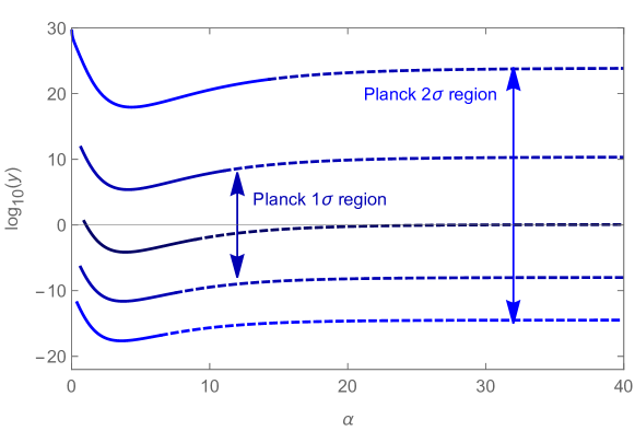
Figure 4: The relation between the inflaton coupling $\mathsf{g}$ and $\alpha$ in the MHI model for different choices of $n_{s}$ marking the $1\sigma$ and $2\sigma$ confidence interval of $n_{s}$  [86]. We here chose the Yukawa coupling $\mathsf{g}=y$, corresponding bounds for other couplings can be obtained with the conversion factors in table 1. We present examples for different couplings in Fig. 26 in the appendix. The dashed lines correspond values of $r$ that exceed the observational upper bound $r<0.06$ from Planck [86]. The relation is non-monotonic for MHI model. Using the upper bound on $r$ one can in principle impose lower (and upper) bound on the inflaton couplings for with given $n_{s}$ without $r$ being measured, though the foreseen sensitivities of LiteBIRD and CMB-S4 will not permit this in practice, cf. Fig. 18. We extend the plot to ludicrously large values of the coupling constants for illustrative purposes, a perturbative treatment is only possible below the horizontal line, and (27) fulfilled for considerably smaller values (typically of the order of the electron Yukawa coupling, cf. Figs. 28 - 31).

The potential of the mutated hilltop inflation (MHI) model [15, 16] has the form

$$\mathcal{V}(\varphi)=M^{4}\left[1-\frac{1}{{\rm cosh}(\varphi/\mu)}\right]~{}=M^{4}\left[1-\frac{1}{{\rm cosh}(\alpha\varphi/M_{pl})}\right]~{}.$$ (35)

Here $M$ represents the typical energy scale for hilltop inflation and $\mu$ is a parameter which has the dimension of mass. It is often convenient to use the dimensionless parameter $\alpha\equiv\mu/M_{pl}$ instead. The potential is shown in Fig. 1, it is asymptotically flat when $|\varphi|$ is large and has a minimum at $\varphi=0$.

Defining the end of inflation as the moment when $\epsilon=1$ we find in terms of $\alpha$

$$\varphi_{\rm end}=\ \alpha M_{pl}\ {\rm arccosh}\frac{3\times 2^{2/3}+2^{1/3}b^{2/3}+2b^{1/3}\alpha+2^{5/3}\alpha^{2}}{6\alpha b^{1/3}}$$ (36)

with $b=3\sqrt{6}a+36\alpha+4\alpha^{3}$ and $a=\sqrt{4\alpha^{4}+22\alpha^{2}-1}$. The inflaton mass $m_{\phi}$ and the self-coupling $\lambda_{\phi}$ of the inflaton can be obtained from the Taylor expansion (20) of its potential near the minimum $\varphi=0$,

$$m_{\phi}=\frac{M^{2}}{\mu}=\frac{M^{2}}{\alpha M_{pl}}~{},\quad g_{\phi}=0~{},\quad\lambda_{\phi}=-\frac{5M^{4}}{\mu^{4}}=-\frac{5M^{4}}{(\alpha M_{pl})^{4}}~{}.$$ (37)

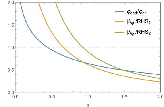
Figure 5: Graphic representation of the conditions on the self-coupling $\lambda_{\phi}$ in the MHI model, which is a function of $\alpha$. We show $\varphi_{\rm end}/\varphi_{\rm cr}$, $\lambda_{\phi}/{\rm RHS}_{1}$ and $\lambda_{\phi}/{\rm RHS}_{2}$, where ${\rm RHS}_{1,2}$ represent the RHS of the two inequalities in (24) as well as (26). These conditions roughly require $\mu>M_{pl}$, i.e., $\alpha>1$.

Parametric dependencies.

We shall first investigate whether the set of parameters $\{M,\alpha,\mathsf{g}\}$ can be uniquely determined from the observables $\{n_{s},A_{s},r\}$. Using (7) we can express $M$ in terms of other parameters and observables,

$$M=M_{pl}\sqrt[4]{\frac{3\pi^{2}rA_{s}}{2[1-1/{\rm cosh}(\varphi_{k}/\mu)]}},$$ (38)

consistent with (69). We do not find an analytic solution for the set of two equations (9) to express $(\varphi_{k},\alpha)$ in terms of $\{r,n_{s}\}$, but we find numerically that such solution exists and is unique within the observationally allowed range of $\{r,n_{s}\}$ and for the values of $\alpha$ that can be made consistent with the conditions (27). This permits to numerically express $\alpha$ in terms of $(n_{s},r)$ and determine $M$ with (38). Hence, the parameters in $\mathcal{V}(\varphi)$ can be fitted without any information on the reheating epoch. Using and (5), (25) and (4) one can in addition determine $N_{k}$ and $N_{\rm re}$. Knowledge of $N_{\rm re}$ already permits to determine the reheating temperature (15). Finally, one can extract the inflaton coupling from (17) and (18) with table 1. Formally one can always extract a value for $\mathsf{g}$ in this way, as $\mathsf{g}$ obtained from (17) and (18) is simply a re-parametrisation of $N_{\rm re}$ (for fixed inflaton potential there is a bijective mapping between $N_{\rm re}$ and $\mathsf{g}$). The parameter $\mathsf{g}$ has a physical meaning as a microphysical coupling constant if the use of (18) on the RHS of (17) is justified, which is the case when (27) are fulfilled. Hence, it is in principle possible to extract all three parameters $\{M,\alpha,\mathsf{g}\}$ from a measurement of $\{n_{s},A_{s},r\}$.

(a)

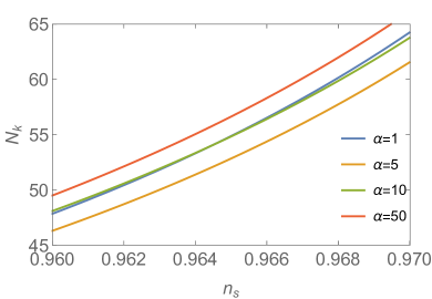
(b)

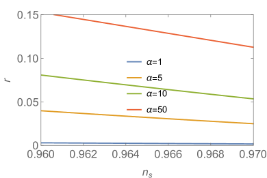
(c)

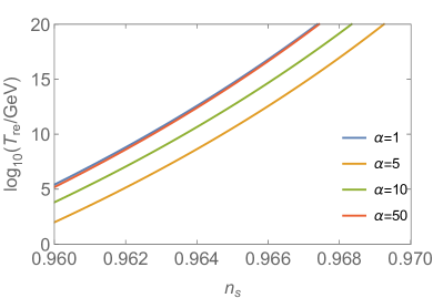
(d)

Figure 6: The $n_{s}$-dependence of $N_{\rm re}$, $N_{k}$, $r$ and $T_{\rm re}$ in the MHI model for various values of $\alpha$. We take $\bar{w}_{\rm re}=0$ as implied by (26) and fixed $A_{s}$ to (34). The colour coding is used to denote different values of $\alpha$.

However, in practice this is difficult even when $r$ is determined by future missions like LiteBIRD and CMB-S4. Fig. 4 shows the dependence of $\alpha$ for different values of $n_{s}$. The different values of $n_{s}$ correspond to the range of $1\sigma$ and $2\sigma$ confidence interval of $n_{s}$ [86]. The tensor-to-scalar ratio $r$ changes monotonically along each curve, and the observational upper Planck bound $r<0.06$ [86] is shown by the separation of solid and dashed lines. Fig. 4 also permits to assess the origin of the uncertainties in the inflaton coupling. On one hand, there is the uncertainty in $r$. A measurement of $r$ would restrict the allowed region to a small fraction of each line in Fig. 4. However, the current error bar on $n_{s}$ translates into a gargantuan uncertainty in the inflaton coupling. Even if $r$ was known with infinite precision (fixing one point along each line in Fig. 4), the uncertainty in $n_{s}$ covers many orders of magnitude in $\mathsf{g}$. This shows that the uncertainty in $n_{s}$ will prohibit a determination of $\mathsf{g}$ with future CMB observations in the MHI model unless further assumptions are made. This is very different from the chaotic inflation model discussed in Sec. 2.4 and simply reflects the fact that models with more free parameters offer more freedom. Hence, in practice we have to fix one parameter in the potential in order to determine $\mathsf{g}$. We choose this parameter to be $\alpha=\mu/M_{pl}$. This is possible because fixing $\alpha$ does not uniquely fix $n_{s}$ and $r$, but only restricts predictions a line in the $n_{s}$-$r$ plane, the position along which is determined by the value of the inflaton coupling $\mathsf{g}$. Each choice of $\alpha$ defines a family of inflaton potentials with one remaining free parameter $M$ that can be fitted to data together with $\mathsf{g}$.

Analysis for fixed $\alpha$.

The Taylor expansion (37) yields $\varphi_{\rm cr}/M_{pl}=\sqrt{\frac{12}{5}}\alpha$. To satisfy the condition (24) $\alpha$ should roughly be larger than unity, cf. Fig. 5. In the following analysis we choose several values of $\alpha$, corresponding to $\alpha=1$,  $5$,  $10$ and $50$. Combining equations (4)-(6) as well as (15) we obtain the $n_{s}$-dependence of four variables in the MHI model: the e-folding number of reheating $N_{\rm re}$, the e-folding number after horizon crossing $N_{k}$, the tensor-to-scalar ratio $r$ and the reheating temperature $T_{\rm re}$, as shown in Fig. 6. These variables have an analytic but complicated dependence on $\alpha$ and $n_{s}$, thus in our work we present the numerical results for different relations in the form of plots.

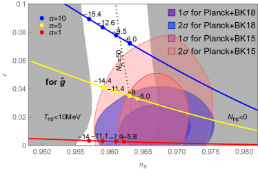
(a)

(b)

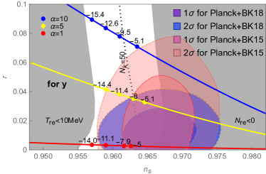
(c)

(d)

Figure 27: Impact of the reheating phase on the predictions of MHI model for $n_{s}$ and $r$ for a set of sample points. In panels [a]-[d] we assume that reheating is primarily driven by an interaction in table 1. The notations are the same with Fig 7.

After eliminating $M$ with (38) and fixing $A_{s}$ to (34), we can compute both $r$ and $\mathsf{g}$ as functions of $n_{s}$ from (17) with table 1. As an example, Fig. 7 shows the impact of the reheating era on the observables $n_{s}$ and $r$ for different values of $\alpha$, assuming an Yukawa coupling. Analogue plots for the other interactions in table 1 are shown in Fig. 27 in the appendix. The distribution of the discs in Fig 8 shows that a determination of $\mathsf{g}$ by measuring $r$ is considerably easier for larger $\alpha$.

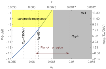
(a)

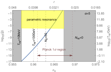
(b)

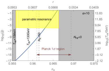
(c)

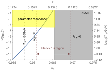
(d)

Figure 28: Dependence of the scalar coupling $\tilde{g}$ on $n_{s}$ in the MHI model for different choices of $\alpha$. The notations are the same with Fig. 8.

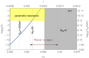
(a)

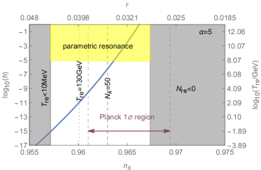
(b)

(c)

(d)

Figure 29: Dependence of the scalar coupling $h$ on $n_{s}$ in the MHI model for different choices of $\alpha$. The notations are the same with Fig. 8.

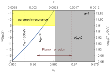
(a)

(b)

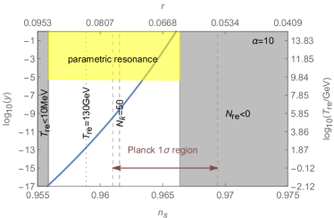
(c)

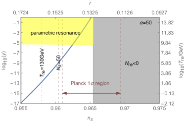
(d)

Figure 30: Dependence of the Yukawa coupling $y$ on $n_{s}$ in the MHI model for different choices of $\alpha$. The notations are the same with Fig. 8.

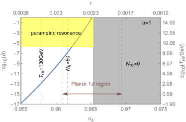
(a)

(b)

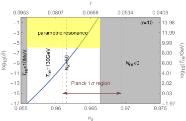
(c)

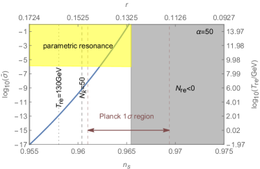
(d)

Figure 31: Dependence of the axion-like coupling $\tilde{\sigma}$ on $n_{s}$ in the MHI model for different choices of $\alpha$. The notations are the same with Fig. 8.

The relation between the inflaton coupling and $n_{s}$ is shown in more detail in Fig. 8, where we have fixed $\alpha=5$ and again assumed an Yukawa coupling. Results for other choices of $\alpha$ and other inflaton interactions are shown in Figs. 28, 29, 30 and 31 in the appendix. The labels on top of the frame show the value of $r$ for given $n_{s}$ and fixed $\alpha$. The labels on the side of each plot indicate the relation between ${\rm log}_{10}(T_{\rm re}/{\rm GeV})$ and ${\rm log}_{10}(\mathsf{g})$ given by (14). This relation is approximately but not exactly linear because the inflaton mass $m_{\phi}$ changes slightly for different choice of parameters. In the yellow region condition (68) is violated. From these figures one can see by eye that a determination of $r$ at the level $\sigma_{r}\sim 10^{-3}$ would be sufficient to constrain the order of magnitude of the inflaton, consistent with what was found in [13]. In the following sections we use two methods to quantify the information gain on $T_{\rm re}$ and $\mathsf{g}$ that can be achieved with CMB-S4 and LiteBIRD.

Finally, it is instructive to consider the case where all parameters in the potential are fixed from theory. For fixed $M$ and $\alpha$ we can use (38) as well as the numerical relation between $n_{s}$ and $r$ obtained from (9) for fixed $\alpha$ to express both $r$ and $n_{s}$ in terms of $A_{s}$. This permits to express $\mathsf{g}$ in terms of the observable $A_{s}$ alone. In Fig. 9 one can see that the current measurement of $A_{s}$ is already sufficient to constrain $\mathsf{g}$ if all parameters in the potential are fixed. We do not further pursue the option to constrain $\mathsf{g}$ in this way, but rather focus on the potential of LiteBIRD and CMB-S4 to simultaneously determine $\mathsf{g}$ and the scale of inflation $M$ from data.

Figure 7: Impact of the reheating phase on the predictions of MHI model for $n_{s}$ and $r$ for a set of sample points. Here we assume an Yukawa inflaton coupling $y$; we show results for all couplings in table 1 in Fig. 27 in the appendix. The red and blue areas display marginalized joint confidence regions for $(n_{s},r)$ at the $1\sigma$ $(68\%)$ CL (dark) and $2\sigma$ $(95\%)$ CL (light) from Planck+BICEP/Keck 2015 and 2018 data, respectively (Fig. 28 in [86] and Fig. 5 in [87], respectively). The predictions of the MHI model with different values of $\alpha$ and $y$ are indicated by the discs. The colour of the disc represents the value of $\alpha$, and the values of ${\rm log}_{10}(y)$ are given by the numbers above the discs. These values have been chosen consistent with condition (68); predictions for other values of $y$ lie on the curve of the same colour, as the choice of $\alpha$ defines a line in the $n_{s}$-$r$ plane. The grey region on the left side corresponds to the lower bound $T_{\rm re}<10$ MeV from BBN in (16), and the grey region on the right side corresponds to $N_{\rm re}<0$. The dotted line corresponds to $N_{k}=50$, which guarantees a sufficient duration of inflation, as specified later in Sec. 4.2.

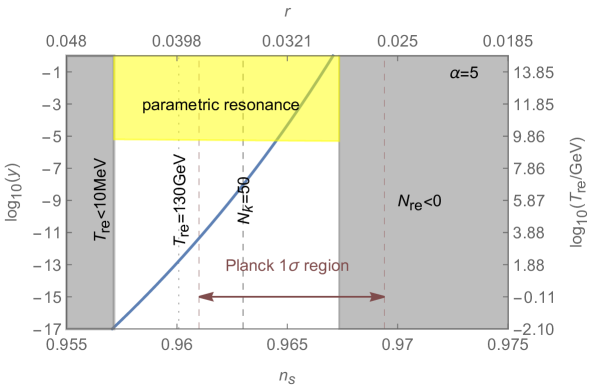
Figure 8: Dependence of the Yukawa inflaton coupling $y$ on $n_{s}$ and $r$ in the MHI model for $\alpha=5$, with the Planck error bar on $n_{s}$ indicated. Results for other values of $\alpha$ and other couplings are shown in Figs. 28-31 in the appendix. On the right of the panels we indicate the value of $T_{\rm re}$ for given $\mathsf{g}$, assuming instantaneous thermalisation. The grey region on the left side corresponds to $T_{\rm re}<10~{}{\rm MeV}$ and is excluded by BBN, and the grey region on the right side corresponds to $N_{\rm re}<0$. The dotted line indicates the electroweak sphaleron freeze-out temperature $T_{\rm re}=131~{}{\rm GeV}$. The region to the right of the dashed line satisfies the requirement $N_{k}>50$. The yellow region, inside which the parametric resonance occurs, gives the upper bound on the inflaton coupling $\mathsf{g}$ from the condition to avoid $\{\mathsf{a}_{i}\}$-dependencies due to feedback caused by resonant particle production. To identify this region we used the more general conditions (68) instead of (27) and neglected a mild dependence on $r$, cf. footnote 15. The red dashed lines represent the $1\sigma$ confidence region of the Planck measurement of $n_{s}$ ($n_{s}=0.9652\pm 0.0042$) after marginalisation over $r$, which should be understood as illustrative (and not taken literally) because $n_{s}$ and $r$ are not independent here, and values of $r$ in the panels labeled [d] in Figs. 28-31 are in fact already disfavoured by the current constraints on $r$ [86, 87].

Figure 9: The Yukawa coupling $y$ as a function of $A_{s}$ for fixed $M$ and $\alpha$ in the MHI model.

3.2 Radion gauge inflation model

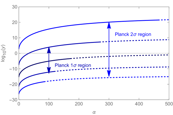
Figure 10: The relation between the inflaton coupling $\mathsf{g}$ and $\alpha$ in the RGI model for different choices of $n_{s}$ marking the $1\sigma$ and $2\sigma$ confidence interval of $n_{s}$. We here chose the Yukawa coupling $\mathsf{g}=y$, with conventions as in Fig. 4. Plot for other couplings are shown in Fig. 32 in the appendix.

The potential of the radion gauge inflation (RGI) model has the form [17, 18]

$$\mathcal{V}(\varphi)=M^{4}\frac{(\varphi/M_{pl})^{2}}{\alpha+(\varphi/M_{pl})^{2}}$$ (39)

Here $M$ represents the typical energy scale for this model and $\alpha$ is a dimensionless parameter. The shape of the potential is shown in Fig. 1. The scale $M$ can again be expressed in terms of other parameters through (7),

$$M=M_{pl}\left(\frac{3\pi^{2}}{2}rA_{s}\left(1+\alpha\frac{M^{2}_{pl}}{\varphi_{k}^{2}}\right)\right)^{1/4},$$ (40)

consistent with (69). Following that, (9) can be solved for $\alpha$,

$$\alpha=\frac{432r^{2}}{(8(1-n_{s})+r)^{2}(4(1-n_{s})-r)}.$$ (41)

As in the MHI model, all parameters in the effective potential (39) can in principle be determined from a measurement of $\{n_{s},A_{s},r\}$ without knowledge about the reheating phase. With the equation of state (25) fixed by the effective potential, the relations (4), (5) and (15) can again be used to determine $N_{\rm re}$ and hence $T_{\rm re}$. This can then finally be converted into a determination of the inflaton coupling $\mathsf{g}$ by means of (17) and table 1, provided that (27) is fulfilled. However, Fig. 10 shows that the uncertainty in $n_{s}$ again prohibits a determination of $\mathsf{g}$ even if $r$ was known exactly unless one specifies $\alpha$.

(a)

(b)

(c)

(d)

Figure 11: Dependence of $N_{\rm re}$, $N_{k}$, $r$ and $T_{\rm re}$ on $n_{s}$ in the RGI model with different values of $\alpha$, in analogy to Fig. 6.

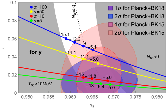
Figure 12: Impact of the reheating phase on the predictions of RGI model for $n_{s}$ and $r$ for a set of sample points and an Yukawa coupling $y$, with conventions as in Fig. 7. Results for other couplings in table 1 in Fig. 33 in the appendix.

The range of allowed values for $\alpha$ is restricted by the conditions to avoid feedback during reheating. Near the minimum $\varphi=0$ of the potential the inflaton mass $m_{\phi}$ and self-couplings are,

$$m_{\phi}=\sqrt{\frac{2}{\alpha}}\frac{M^{2}}{M_{pl}}~{},\quad g_{\phi}=0~{},\quad\lambda_{\phi}=-\frac{24M^{4}}{\alpha^{2}M^{4}_{pl}}~{}.$$ (42)

With (26) this gives $\varphi_{\rm cr}=\sqrt{\alpha}M_{pl}$. Comparing this to

$$\varphi_{\rm end}=M_{pl}\frac{a^{1/3}-\alpha}{\sqrt{3}a^{1/6}}$$ (43)

with $a=\alpha^{2}(27+\alpha+3\sqrt{81+6\alpha})$ the condition $\varphi_{\rm end}<\varphi_{\rm cr}$ in (26) translates into $\alpha>1/2$. Condition (24) implies $\alpha>2.37$. In our analysis $\alpha$ is chosen to be four values: $\alpha=5,~{}10,~{}50$ and 100. For fixed $\alpha$ we can get the $n_{s}$-dependence of $N_{\rm re}$, $N_{k}$, $r$ and $T_{\rm re}$ in RGI model, as shown in Fig. 11. If we fix $n_{s}$ we can express the inflaton coupling in terms of $\alpha$. The dependence is monotonic, as can been seen in Fig. 10. The different curves in each panel correspond to different values of $n_{s}$, and $r$ changes along each curve.

Fig. 12 shows the impact of the reheating epoch on the model predictions in the $n_{s}$-$r$ plane together with the Planck+BICEP2/Keck 2015 and 2018 results [86, 87] ($1\sigma$ and $2\sigma$ CL). The corresponding values of ${\rm log}_{10}\mathsf{g}$ are indicated by the numbers above the discs, and different values of $\alpha$ are distinguished by color coding (same as in Fig. 7). Finally, the dependence of the inflaton coupling on $n_{s}$ and $r$ is shown in Fig. 13.

Figure 13: Dependence of the Yukawa coupling $y$ on $n_{s}$ and $r$ in the RGI model for $\alpha=100$ with conventions as in Fig. 8. Results for other couplings are shown in Figs. 34, 35, 36, 37 in the appendix.

Figure 14: The relation between the inflaton coupling $\mathsf{g}$ and $\alpha$ in the $\alpha$-T model for different choices of $n_{s}$ marking the $1\sigma$ and $2\sigma$ confidence interval of $n_{s}$. We again chose the Yukawa coupling $\mathsf{g}=y$, with conventions as in Fig. 4. Plot for other couplings are shown in Fig. 32 in the appendix.

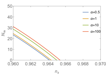
(a)

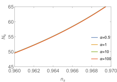
(b)

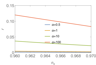
(c)

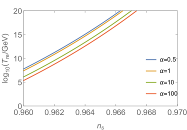
(d)

Figure 15: Dependence of $N_{\rm re}$, $N_{k}$, $r$ and $T_{\rm re}$ on $n_{s}$ in the $\alpha$-T model with different values of $\alpha$, in analogy to Fig. 6.

3.3 $\alpha$-attractor T-model

The so-called $\alpha$-attractor models [103] represent a broad class of popular inflationary models. For some of them constraints on the inflaton coupling have previously been derived in [40, 43, 48]. Here we focus on the so-called T-type models, which have a symmetric potential. In E-type models it is much more difficult to obtain a bound on $\mathsf{g}$ because self-interactions tend to violate (24), cf. appendix C. The potential of the $\alpha$-attractor T-models ($\alpha$-T) [19, 20, 21] has the form

$$\mathcal{V}(\varphi)=M^{4}{\rm tanh}^{2n}\left(\frac{\varphi}{\sqrt{6\alpha}M_{pl}}\right)$$ (44)

Here $M$ is the typical energy scale for this model and $\alpha$ is a dimensionless parameter. The shape of the potential shown in Fig. 1. The scale $M$ can again be expressed in terms of other parameters with the help of (7),

$$M=M_{pl}\left(\frac{3\pi^{2}}{2}A_{s}r\right)^{1/4}\tanh^{-\frac{n}{2}}\left(\frac{\varphi_{k}}{\sqrt{6\alpha}M_{pl}}\right),$$ (45)

consistent with (69). Again defining the end of inflation as the moment when $\epsilon=1$ we find

$$\varphi_{\rm end}=\frac{M_{pl}}{2}\sqrt{\frac{3\alpha}{2}}{\rm ln}\left(\frac{3\alpha+8n^{2}+4n\sqrt{4n^{2}+3\alpha}}{3\alpha}\right)$$ (46)

To ensure a parabolic potential near the minimum and fulfil condition (26) we have to choose $n=1$. With the help of (9) we find

$$\alpha=\frac{4r}{3(1-n_{s})(4(1-n_{s})-r)}.$$ (47)

As in the other models, the formalism outlined in Sec. 2 can in principle be used to constrain $T_{\rm re}$ as a function of $n_{s}$ or $r$. However, as in the other examples, in practice the large uncertainty in $n_{s}$ makes it practically impossible to determine all parameters in the potential from observation (cf. Fig. 14), and one has to fix $\alpha$ from model-building considerations.

In order to identify the range of values consistent with the conditions (24) and (26) we Taylor expand $\mathcal{V}(\varphi)$ according to (20) and identify

$$m_{\phi}=\frac{M^{2}}{\sqrt{3\alpha}M_{pl}}\ ,\ g_{\phi}=0\ ,\ \lambda_{\phi}=-\frac{4M^{4}}{9\alpha^{2}M^{4}_{pl}}~{}.$$ (48)

The quadratic term in (20) dominates over the quartic term at the end of inflation if $\alpha>0.04$. For $\alpha>0.25$ condition (24) can be fulfilled. Fig. 15 shows the $n_{s}$-dependence of $N_{\rm re}$, $N_{k}$, $r$ and $T_{\rm re}$ for these values of $\alpha$.

Figure 16: Impact of the reheating phase on the predictions of $\alpha$-T model for $n_{s}$ and $r$ for a set of sample points and an Yukawa coupling $y$, with conventions as in Fig. 7. Results for other couplings in table 1 in Fig. 39 in the appendix.

In our analysis $\alpha$ is chosen to be $0.5,~{}1,~{}10,$ and $100$. Fig 16 compares the model predictions in the $n_{s}$-$r$ plane to the Planck+BICEP2/Keck 2015 and 2018 results [86, 87] ($1\sigma$ and $2\sigma$ CL). The corresponding values of ${\rm log}_{10}\mathsf{g}$ are indicated by the numbers over the discs, and different choices of $\alpha$ distinguished by color of the discs, following the notation of Fig. 7. We find that observational data slightly disfavours values of the inflaton coupling where conditions (27) are fulfilled. Finally, the dependence of the inflaton couplings on $n_{s}$ is shown in Fig. 17.

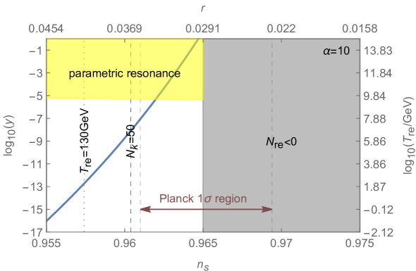
Figure 17: Dependence of the Yukawa coupling $y$ on $n_{s}$ and $r$ in the $\alpha$-T model for $\alpha=10$ with conventions as in Fig. 8. Results for other couplings are shown in Figs. 40, 41, 42, 43 in the appendix.

4 Methods for estimating the LiteBIRD and CMB-S4 sensitivities

In the previous section we have studied the relations between the fundamental model parameters $\{M,\alpha,\mathsf{g}\}$, the physical scales $\{M,m_{\phi},T_{\rm re}\}$ and the properties of the observable CMB perturbations characterised by $\{n_{s},A_{s},r\}$. In the following sections we will investigate how much information about the fundamental parameters and physical scales can be gained with observations of LiteBIRD and CMB-S4. Our task is straightforwardly phrased in the language of Bayesian statistics. We have some knowledge on a set of fundamental parameters $X$ from observation and theoretical consistency specified in Sec. 4.2 that we can use to define a prior $P(X)$. This knowledge will be confronted with new data $\mathcal{D}$, which we can characterise by a likelihood function $P(\mathcal{D}|X)$. Then the posterior distribution for $X$ is given by

$$P(X|\mathcal{D})=P(\mathcal{D}|X)P(X)/P(\mathcal{D}),$$ (49)

with $P(\mathcal{D})=\int dXP(\mathcal{D}|X)P(X)$. In principle the set of parameters that we are interested in is $X=\{M,\alpha,\mathsf{g}\}$, but in practice we will always fix $\alpha$. In the following we use two different methods to evaluate (49).

• In section 4.3 we use the analytic method introduced in [14]. In this approach $A_{s}$, $n_{s}$ and $r$ are considered observables, i.e., $\mathcal{D}=\{n_{s},A_{s},r\}$.

• In section 4.4 we perform full-fledged forecasts in which $\mathcal{D}$ is a set of generated CMB mock-spectra for given true values of $\mathsf{g}$ and $M$. In addition, the set $X$ then contains the parameters of the concordance model of cosmology, cf. (58).

Before applying these methods we need to specify the sub-classes of models we want to consider, in particular the choice of $\alpha$ in each of the categories MHI, RGI and $\alpha$-T models.

4.1 Model class selection: choosing $\alpha$

If $\{n_{s},A_{s},r\}$ could be measured without uncertainties, then $M$, $\alpha$ and $N_{\rm re}$ can be determined unambiguously in the class of models considered here. This permits to identify the physical scales via a mapping

$$\{n_{s},A_{s},r\}\leftrightarrow\{M,m_{\phi},T_{\rm re}\},$$ (50)

using the general formalism presented in Sec. 2.2 as well as the relations for each model given in Sec. 3. The inflaton coupling $\mathsf{g}$ can in general only be extracted from data if many parameters $\{\mathsf{a}_{i}\}$ in the underlying particle physics model are specified. However, if conditions in appendix B are fulfilled, then the formalism summarised in Sec. 2.3 further permits to determine $\mathsf{g}$ unambiguously, i.e., there is a mapping

$$\{n_{s},A_{s},r\}\leftrightarrow\{M,m_{\phi},T_{\rm re}\}\leftrightarrow\{M,\alpha,\mathsf{g}\}.$$ (51)

However, in practice one will not be able to determine $\{n_{s},A_{s},r\}$ exactly from data. One result that is common to all classes of models in Sec. 3 is that current and near-future observational information on the quantities $\{A_{s},n_{s},r\}$ will not be sufficient to simultaneously fit all microphysical parameters $\{M,\alpha,\mathsf{g}\}$ because the error bar on $n_{s}$ is too large. This can e.g. be seen by comparing Figs. 4, 10 and 14 to Fig. 18. In terms of energy scales this means that one cannot observationally determine $\{M,m_{\phi},T_{\rm re}\}$ within a class of models without making at least some additional assumptions. It may be that the situation improves if further properties of the CMB spectra are taken into account (such as the running of $n_{s}$ or non-Gaussianities). However, since the relation between those properties and the microphysical parameters $\{M,\alpha,\mathsf{g}\}$ has not been studied in detail yet, we take the approach to consider families of inflationary models with fixed $\alpha$. This establishes a relation between the inflaton mass $m_{\phi}$ and the scale of inflation $M$, with the latter being the sole free parameter in the potential $\mathcal{V}(\varphi)$ in each family of models. Since fixing $\alpha$ fixes the inflaton mass as a function of $M$ (cf. (37), (42), (48)), we practically determine $\{M,\mathsf{g}\}$ from data, and $m_{\phi}$ is then fixed by $M$ and the choice of $\alpha$. Further, fixing $\alpha$ establishes a relation between $n_{s}$ and $r$, implying that the predictions for each family of models are restricted to a line in the $n_{s}$-$r$-plane (cf. Figs. 7, 12 and 16). $M$ and $\mathsf{g}$ vary along this line, and the accuracy by which they can be constrained depends on the sensitivity of future experiments to $n_{s}$ and $r$. In practice the information gain that can be achieved with CMB-S4 and LiteBIRD will primarily be driven by their sensitivity to $r$.

Our primary goal is to quantify the information gain on $T_{\rm re}$ and $\mathsf{g}$ that can be obtained with LiteBIRD and CMB-S4. For our study, we select values of $\alpha$ for which the following conditions are fulfilled:

• The line in the $n_{s}$-$r$-plane defined by this choice of $\alpha$ in a given family of models crosses the region favoured by current constraints.

• The conditions (24) can be fulfilled.

• The resulting line in the $n_{s}$-$r$-plane is steep enough that a sensitivity $\sigma_{r}\sim 10^{-3}$ can be sufficient to determine the order of magnitude of $\mathsf{g}$. The is generally the case if $r\sim 10^{-2}$ or larger.

Our choice of values is summarised in table 2 together with other parameters relevant for the method described in Sec. 4.4.

model	$\alpha$	${\rm log}_{10}(\bar{y})$	prior range ${\rm log}_{10}(y)$	$\bar{M}[M_{\text{pl}}]$	prior range $M[M_{\text{pl}}]$	$\bar{n}_{s}$
MHI	3.4	-6.32	$<0.59$	0.005193	$\left[0.0050,0.0054\right]$	0.9640
RGI	19	-6.82	$<0.58$	0.005296	$\left[0.0051,0.0055\right]$	0.9669
$\alpha$-T	6	-1.03	$<0.60$	0.005182	$\left[0.0050,0.0054\right]$	0.9641

Table 2: Fiducial values of ${\rm log}_{10}(y)$ and $M$ (${\rm log}_{10}(\bar{y})$ and $\bar{M}$) and their prior ranges, for the different models under consideration.

4.2 Knowledge prior to observation

In order to quantify the knowledge gain that can be achieved with LiteBIRD or CMB-S4, we must first quantify the current knowledge, which is needed to define a Bayesian prior. We consider three types of information

• Model choice and parametrisation. Even if no explicit prior $P(X)$ is imposed, the parametrisation of $\mathcal{V}$ in terms of the $\{\mathsf{v}_{i}\}\subset X$ induces a metric in the mapping between $\mathcal{D}$ and $X$, and $P(\mathcal{D}|X)$ in general is not invariant under changes in the parametrisation. While this is not represent a Bayesian prior in the strict sense, it does reflect prior assumptions about what the fundamental parameters in nature are, and this has an impact on the posteriors.

• Overall geometry of the universe. One of the main motivations for cosmic inflation comes from the observation that the observable universe is homogeneous and isotropic on large scales. Explaining this observation imposes a lower bound on the duration of inflation in terms of $e$-folds, and hence also a lower bound on $N_{k}$. The precise value of this bound depends a bit on the specific problem that one wants to solve (cf. e.g. [104, 105, 106]). For the sake of definiteness we impose

  $$N_{k}>50,$$ (52)

  which is consistent with the lower bound has been used by the Planck collaboration, cf. Fig. 8 in [107]. Note that, while the precise value used in (52) can be a matter of debate, conceptually this is a hard observational bound (based on the observation that the universe is homogeneous, isotropic, and spatially flat), and not a theoretical criterion. It should also be noted that this piece of information does not come from any of the study of the spectrum of CMB perturbations, but can be inferred from the high level of isotropy of the CMB, which was known prior to the missions that studies the spectrum of perturbations.

• Previous measurements of the CMB power spectrum. The power spectrum of CMB anisotropies has been studied by a number of probes, with the most recent one being the combined analysis of Planck, WMAP, and BICEP/Keck observations in [87]. This data was obtained from the same CMB that will be studied by CMB-S4 and LiteBIRD, hence it strictly speaking does not represent independent information. To avoid complications related to combining correlated data in a Bayesian analysis we refrain from including this information into our priors. Practically this has little consequences, as it has been estimated in [14] that the bounds on $r$ and $n_{s}$ reported in [87] do not impose a significant constraint on $\mathsf{g}$ or $T_{\rm re}$.

• Requirement to actually reheat the universe. Using (13), the lower bound (16) on $T_{\rm re}$ from BBN can be converted into a lower bound on $\mathsf{g}$ [13],

  $$\mathsf{g}>g_{*}^{1/4}\frac{T_{\rm BBN}}{\sqrt{m_{\phi}M_{pl}}}\sqrt{\#}\simeq\frac{T_{\rm BBN}}{M_{pl}}\left(\frac{g_{*}}{A_{s}r}\right)^{1/4}\sqrt{\#}.$$ (53)

  The second relation in (53) is approximately valid for plateau models of inflation, as those considered in this work. Most baryogenesis scenarios and Dark Matter production mechanisms require temperatures considerably above $T_{\rm BBN}$, cf. footnote 12. However, given our ignorance about baryogenesis and Dark Matter, we impose the conservative bound $T_{\rm re}>T_{\rm BBN}$. A lower bound $\mathsf{g}$ from any other lower bound on $T_{\rm re}$ can be obtained trivially from (53) by replacing $T_{\rm BBN}$ with the respective temperature.

• Physical consistency. Physical consistency obviously requires $N_{\rm re}\geq 0$. In contrast to (52) this constraint has no uncertainty or tolerance (cf. footnote 19), but must be modelled by a prior $P(N_{\rm re})\propto\theta(N_{\rm re})$. Conceptually it may be more appropriate to view this as a condition that defines the boundaries of the range of values for $\{M,\alpha,\mathsf{g}\}$ (and not as a prior, as it is not derived from any prior observation, but from physical consistency alone).

4.3 A simple analytic method

In this section we briefly review the method introduced in [14]. In this method the set of observables $\mathcal{D}$ in principle comprises $A_{s}$, $n_{s}$ and $r$. For illustrative purposes we keep $A_{s}$ fixed to (34) and determine $M$ from (7), cf. (38), (40) and (45). This is not strictly necessary for this method to be applied, but conveniently reduces (49) to a one-dimensional integral with $X={\rm log}_{10}\mathsf{g}$ and $\mathcal{D}=\{n_{s},r\}$ (as $A_{s}$, $n_{s}$, $r$, $N_{k}$ and $N_{\rm re}$ are functions of $\mathsf{g}$ alone, leaving aside the small disclaimers mentioned in footnote 11). We a posteriori find that the validity of the method is not significantly reduced by this simplification, cf. Fig. 23. A prior probability density function for $\mathsf{g}$ (more precisely: $x={\rm log}_{10}\mathsf{g}$) can be constructed from

$$P(x)=c_{1}P\big{(}N_{k}(x)\big{)}\ \gamma(x)\ \theta\big{(}N_{\rm re}(x)\big{)}\ \theta\big{(}T_{\rm re}(x)-T_{\rm BBN}\big{)},$$ (54)

with $P(N_{k})\propto\theta(N_{k}-50)$, $\theta$ the Heaviside function, and $\gamma$ a function that allows for a re-weighting of the prior $P(x)$. The constant $c_{1}$ can be fixed from the requirement $\int dxP(x)=1$. To define a likelihood function we use a two-dimensional Gaussian in $n_{s}$ and $r$ with mean values $\bar{n}_{s}$ and $\bar{r}$ and variances $\sigma_{n_{s}}^{2}$ and $\sigma_{r}^{2}$,

$$\mathcal{N}(n_{s},r|\bar{n}_{s},\sigma_{n_{s}};\bar{r},\sigma_{r})=\frac{1}{2\pi\sigma_{n_{s}}\sigma_{r}}{\rm exp}\left(-\frac{1}{2}\left(\frac{n_{s}-\bar{n}_{s}}{\sigma_{n_{s}}}\right)^{2}\left(\frac{r-\bar{r}}{\sigma_{r}}\right)^{2}\right).$$ (55)

The Gaussian approximation appears to be justified by the shape of the exclusion regions reported by past CMB observations, such as [87]. In (55) we have in addition assumed a diagonal covariance matrix. While this assumption is not exactly correct, it turns out that it does not lead to a significant loss of accuracy when it comes to the posterior for $x$. In [14] $\sigma_{n_{s}}$ and $\sigma_{r}$ were obtained from the sensitivities quoted in the literature for both, LiteBIRD [76] and CMB-S4 [8]. This extraction is not trivial because these sensitivities depend on the true values of $n_{s}$ and $r$ (and also on the assumptions regarding delensing etc), and the complete information about the expected relations is not public. In the present work we obtain $\sigma_{n_{s}}$ and $\sigma_{r}$ by performing forecasts as described in Sec. 4.4 with $n_{s}$ and $r$ as free MCMC parameters. Assuming $\bar{n}_{s}=0.967$ and $\bar{r}=0.02$ as fiducial values we find $\sigma_{n_{s}}=0.0041$ and $\sigma_{r}=0.0013$. The corresponding contours in the $n_{s}$-$r$ plane are shown in Fig. 18. The complete likelihood function then reads (recall that $\mathcal{D}=\{n_{s},r\}$ here)

$$P(\mathcal{D}|x)=c_{2}\mathcal{N}(n_{s}(x),r(x)|\bar{n}_{s},\sigma_{n_{s}};\bar{r},\sigma_{r})\theta(r)\tilde{\gamma}(x),$$ (56)

where $\tilde{\gamma}$ another weighting function and the constant $c_{2}$ is fixed by normalising $P(\mathcal{D}|x)$ to unity. In the following we use $\gamma=\tilde{\gamma}=1$ after checking that the conclusions remain unchanged when using $\gamma=\frac{dN_{\rm k}}{dx}$ or $\tilde{\gamma}=((\frac{dn_{s}}{dx})^{2}+(\frac{dr}{dx})^{2})^{1/2}$. The posterior for $x$ is then obtained from (49) with (54) and (56),

$$P(x|\mathcal{D})=P(\mathcal{D}|x)P(x)/P(\mathcal{D}).$$ (57)

The resulting posteriors for the three models under consideration can be seen in Fig. 22 to 24 together with the results from the next section.

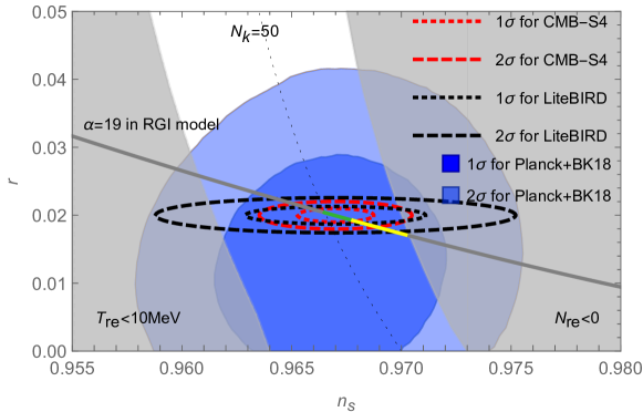
Figure 18: The ellipses indicate the likelihood (55) as a function of $n_{s}$ and $r$, with $\bar{n}_{s}=0.967$, $\bar{r}=0.02$ and $\sigma_{n_{s}}=0.0017$, $\sigma_{r}=0.0010$ for CMB-S4 and $\sigma_{n_{s}}=0.0041$, $\sigma_{r}=0.0013$ for LiteBIRD (found with the forecast method from Sec. 4.4 with $n_{s}$ and $r$ as free MCMC parameters.) The diagonal line is given by (41) with $\alpha=19$. The colourful part of this line corresponds to the region where $N_{k}>50$ and $N_{\rm re}>0$. In the green part in addition (68) is fulfilled. All other conventions as as in Fig. 7.

4.4 Forecast Method

As explained in Sec. 3, the fundamental parameters ${\rm log}_{10}(y)$, $M$ and $\alpha$ can be mapped into the phenomenological parameters $A_{s}$, $n_{s}$ and $r$ which are conventionally used in the context of the CMB. For the reasons discussed in Sec. 4.1, a simultaneous measurement of all three parameters $\{M,\alpha,\mathsf{g}\}$ from $\{A_{s},n_{s},r\}$ will not be possible neither with LiteBIRD nor with CMB-S4. Therefore, we fix the value of $\alpha$ according to the criteria described at the end of Sec. 4.1 while ${\rm log}_{10}(y)$ and $M$ are allowed to vary freely in our analysis. The corresponding choices for $\alpha$ for the different models considered in this work are summarised in Tab. 2. This means that our analysis has in total 6 free MCMC parameters, i.e.

$$X=\{\omega_{\mathrm{b}},\omega_{\mathrm{cdm}},100\theta_{\mathrm{s}},\tau_{\mathrm{reio}}\}+{\rm log}_{10}(y)+M\,,$$ (58)

where the first 4 parameters are the standard $\Lambda$CDM base parameters, namely the baryon density $\omega_{\mathrm{b}}$, the cold dark matter density $\omega_{\mathrm{cdm}}$, the sound horizon at recombination $\theta_{\mathrm{s}}$ and the optical depth to reionization $\tau_{\mathrm{reio}}$. We modified the linear Boltzmann-Einstein solver class [109] (which calculates the CMB anisotropy spectrum) such that it takes ${\rm log}_{10}(y)$ and $M$ as free input parameters while the values of $A_{s}$, $n_{s}$ and $r$ are inferred from them. This requires to create numerical tables for $A_{s}$, $n_{s}$ and $r$ on a grid of ${\rm log}_{10}(y)$ and $M$ values. The step size both of $M$ and ${\rm log}_{10}(y)$ was chosen carefully such that it corresponds to less than $0.2$ of the expected standard deviations in $A_{s}$, $n_{s}$ and $r$. The range of the covered ${\rm log}_{10}(y)$ and $M$ values was chosen such that it covers around $10$ of the expected standard deviations in $A_{s}$, $n_{s}$ and $r$. We implemented a routine in class that interpolates between the ${\rm log}_{10}(y)$ and $M$ values in this table such that the code can interpret any arbitrary value of ${\rm log}_{10}(y)$ and $M$ (inside the covered range).

$\bar{\omega}_{\mathrm{b}}$	$\bar{\omega}_{\mathrm{cdm}}$	$100\bar{\theta}_{\mathrm{s}}$	$\bar{\tau}_{\mathrm{reio}}$
0.02237	0.1200	1.04092	0.0544

Table 3: Fiducial values for the 4 base $\Lambda$CDM parameters.

In order to perform the forecast, we used the built-in forecast tool provided by the Monte Carlo Markov Chain (MCMC) engine MontePython [22, 23]. Mock likelihoods both for CMB-S4 and LiteBIRD are as well already built-in (originally developed for [110]) and we here assume the same experimental specifications as in [111]. Note that for CMB-S4 this implies that we assume a sky coverage of $f_{\text{sky}}=0.4$ whereas the latest CMB-S4 science book [8] assumes $f_{\text{sky}}=0.01$. As explained in [8], the optimal choice of $f_{\text{sky}}$ is not only subject to a complicated interplay between raw sensitivity, the ability to remove foregrounds and the ability to delense - but it also depends on the true value of $r$ which is assumed to be $\bar{r}=0$ throughout [8]. The CMB-S4 deep survey is therefore designed such that the sky coverage can be increased in case of a detection of $r$. Our choices for the true values of ${\rm log}_{10}(y)$ and $M$ (i.e. the fiducial values $\bar{x}$ and $\bar{M}$) in Tab. 2 implies $\bar{r}\sim 0.02$, which justifies the choice of a larger sky fraction and we stick to $f_{\mathrm{sky}}=0.4$ as in [111]. At the same time, while for small values of $\bar{r}$ and $f_{\mathrm{sky}}$ the sensitivity on $r$ crucially depends on the success of delensing, successful delensing is not that crucial for $f_{\mathrm{sky}}=0.4$ and $r=0.02$ (see fig. 8 in [112]). In our forecast, we assume both successful delensing as well as no delensing at all for the creation of the CMB-S4 mock likelihoods. For LiteBIRD in contrast, we assume no delensing due to its restricted delensing capabilities (which is also the assumption in [110]).

As described in [23], the MontePython forecast method basically consists of 3 steps:

• Mock data for the fiducial model are created. The fiducial values for the 4 base parameters can be found in Tab. 3 and the fiducial values for ${\rm log}_{10}(y)$ and $M$ in Tab. 2. The values for ${\rm log}_{10}(\bar{y})$ and $\bar{M}$ are chosen in a way that one can expect the resulting value of $A_{s}$ near (34) and the values of $n_{s}$ and $r$ inside the region allowed by current observations, based on the formulae in Sec. 3. It has been shown in [113] that scattering of the mock data (due to cosmic variance) can be neglected.

• The Fisher matrix and its inverse are derived. In case of Gaussian likelihoods, the standard deviations for the parameters in Eq. (58) are directly given by the square roots of the diagonal elements of the inverse Fisher matrix. However, as shown in [113], in general this does not hold for non-Gaussian likelihoods and in particular in presence of parameter degeneracies (as is expected for ${\rm log}_{10}(y)$ and $M$). We therefore proceed with iii).

• MCMCs are produced, where the inverse Fisher matrix is used as a covariance matrix; the resulting chains are analyzed either with the built-in analysis tool of MontePython or with the analysis tool GetDist [114] (which we used to create the posterior plots in figs. 19,20 and 21). As discussed in Sec. 4.2, the condition $N_{\mathrm{re}}\gtrsim 0$ imposes a hard cut on ${\rm log}_{10}(y)$ which can be found in table 2. Even though just as well physically motivated, the precise definition of the the other priors discussed in Sec. 4.2 is somewhat more flexible. We therefore decided to not impose these priors at the level of creating the MCMCs but only take them into account afterwards. The prior on $M$ in Tab. 2 is of practical nature and has no physical significance (and also does not affect our results), it simply reflects the range of $M$ covered by our numerical table. Note that the translation of the conditions $N_{\rm re}>0$ and $N_{k}>50$ into a boundary for ${\rm log}_{10}(y)$ in general depends on the value of $M$ (which is varied freely in our analysis). We have however checked that the prior boundary of ${\rm log}_{10}(y)$ only varies mildly over the prior range of $M$, such that we can simply ignore this dependency in our analysis.

5 Results and Discussion

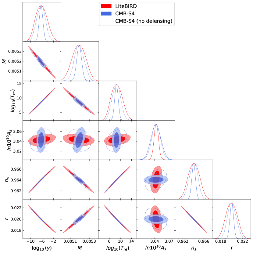
Figure 19: Marginalized 1d- and 2d-posterior distributions for ${\rm log}_{10}(y)$, $M$ and the derived parameters $T_{\rm re}$, $\ln(10^{10}A_{s})$, $n_{s}$ and $r$ for the MHI model.

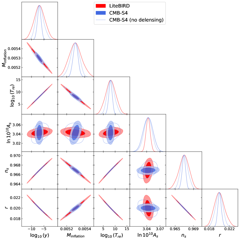
Figure 20: Same as fig. 19 but for the RGI model.

Figure 21: Same as fig. 19 but for the $\alpha-T$ model.

The results of our forecast can be found in Fig. 19 (MHI model), Fig. 20 (RGI model) and Fig. 21 ($\alpha$-T) in form of 2d- and 1d- marginalized posterior distributions for ${\rm log}_{10}(y)$ and $M$. We also show the resulting posterior distributions for the derived parameters ${\rm ln}(10^{10}A_{s})$, $n_{s}$ and $r$, along with the posterior distribution for the reheating temperature $T_{\mathrm{re}}$. The reheating temperature can be calculated from inserting Eq. (18) into Eq. (13),

$$T_{\rm re}=\left\{\begin{aligned} &&yM\frac{1}{\sqrt{8\pi\alpha}}\left(\frac{90}{\pi^{2}g_{*}}\right)^{1/4}\quad{\rm for\ MHI},\\ &&yM\frac{1}{\sqrt{8\pi\sqrt{\alpha/2}}}\left(\frac{90}{\pi^{2}g_{*}}\right)^{1/4}\quad{\rm for\ RGI},\\ &&yM\frac{1}{\sqrt{8\pi\sqrt{3\alpha}}}\left(\frac{90}{\pi^{2}g_{*}}\right)^{1/4}\quad{\rm for}\ \alpha-T.\end{aligned}\right.$$ (59)

Figs. 19-21 show clearly that CMB-S4 as well as LiteBIRD are expected to simultaneously constrain the scale of inflation $M$ as well as the reheating temperature $T_{\rm re}$.

In general, the figures show that CMB-S4 is expected to have higher sensitivity on ${\rm log}_{10}(y)$ and $M$ than LiteBIRD – to which extent however strongly depends on the success of delensing. The only parameter in Figs. 19, 20 and 21 that is more constrained by LiteBIRD than by CMB-S4 is the scalar amplitude $A_{s}$. At scales below the reionization bump, $\ell\gtrsim 10$, there is a strong degeneracy between $A_{s}$ and the optical depth to reionization $\tau_{\mathrm{reio}}$. This degeneracy is removed in case of LiteBIRD (which is designed to measure exactly this reionization bump) but not in case of CMB-S4 which will provide no measurement at these largest scales. It is worthwhile noting that due to the different scales observed by LiteBIRD and CMB-S4, the two experiments are considered to be complementary. It is therefore expected that combining data from both will lead to an improved determination of $T_{\rm re}$ and ${\rm log}_{10}(y)$. Due to complications related to partially overlapping data sets, we however do not perform such a combined analysis.

model	${\rm log}_{10}(y)$	$M[M_{\text{pl}}]$	${\rm log}_{10}(T_{\text{re}}[\text{GeV}])$
MHI	$-5.39\pm 1.52$	$0.00516\pm 0.00005$	$9.49\pm 1.51$
RGI	$-5.56\pm 1.44$	$0.00526\pm 0.00005$	$9.34\pm 1.44$
$\alpha$-T	$-1.70\pm 1.43$	$0.00521\pm 0.00005$	$13.13\pm 1.43$

Table 4: Expected 1 $\sigma$ sensitivities on the inflaton coupling $y$, $M$ and the reheating temperature $T_{\rm re}$ for LiteBIRD. The values in brackets are without delensing. Here we considered a Yukawa coupling $y$, corresponding ranges for other types of interactions can be obtained with table 1.

model	${\rm log}_{10}(y)$	$M[M_{\text{pl}}]$	${\rm log}_{10}(T_{\text{re}}[\text{GeV}])$
MHI	$-6.28\pm 0.63$   $\left(-5.80\pm 1.19\right)$	$0.00519\pm 0.00002$   $\left(0.00518\pm 0.00004\right)$	$8.59\pm 0.63$   $\left(9.08\pm 1.19\right)$
RGI	$-6.67\pm 0.57$   $\left(-5.97\pm 1.14\right)$	$0.00529\pm 0.00002$   $\left(0.00527\pm 0.00004\right)$	$8.23\pm 0.57$   $\left(8.93\pm 1.14\right)$
$\alpha$-T	$-1.03\pm 0.62$   $\left(-1.62\pm 1.32\right)$	$0.00518\pm 0.00002$   $\left(0.00520\pm 0.00005\right)$	$13.80\pm 0.62$   $\left(13.20\pm 1.32\right)$

Table 5: Expected 1 $\sigma$ sensitivities on the inflaton coupling $y$, $M$ and the reheating temperature $T_{\rm re}$ for CMB-S4. The values in brackets are without delensing. Here we considered a Yukawa coupling $y$, corresponding ranges for other types of interactions can be obtained with table 1.

Except for the prior $N_{\rm re}>0$ we have not imposed any other of the priors discussed in Sec. 4.2 in order to produce Figs. 19, 20 and 21. These figures therefore mainly reflect the experiments’ pure sensitivity towards ${\rm log}_{10}(y)$ and $M$. We also added enlarged figures for the 1-d posterior distribution of ${\rm log}_{10}(y)$ in Figs. 22, 23 and 24, along with the different priors discussed in Sec. 4.2. The top x-axis displays the reheating temperature $T_{\rm re}$. In general, $T_{\rm re}$ as well as the different prior conditions are all $M$ dependent. We however checked that – given the very narrow allowed $M$ range – this $M$ dependence is negligible and we can simply fix $M$ to its fiducial value in Tab. 2 in order to produce Figs. 22, 23 and 24. In all cases the prior $N_{k}>50$ turns out to be more stringent than the $T_{\rm re}>10$ MeV prior. Tab. 4 displays $1\sigma$ sensitivities for ${\rm log}_{10}(y)$, $M$ and $T_{\rm re}$ after the $N_{k}>50$ prior has been imposed. They show that both CMB-S4 and LiteBIRD have the capacity to simultaneously measure the scale of inflation $M$ and the reheating temperature $T_{\rm re}$ within class of potentials characterised by a choice of $\alpha$. For the parameters chosen here the order of magnitude of the inflaton coupling can also be measured in the MHI and RGI models, as the peaks of the posteriors fall into the white regions in Figs. 22 and 23. In the $\alpha$-T model condition (27) is violated for the fiducial value of the inflaton coupling $\bar{y}$ that we picked in order to bring the predictions for $n_{s}$ and $r$ into a regime that is allowed by current observations. Hence, the values for $\mathsf{g}$ given in tables  4 and 5 for the $\alpha$-T model cannot be interpreted as measurements of an actual microphysical parameter, but should rather be seen as proxies for $T_{\rm re}$.

The blue discs in Fig. 16 indicate that there are parameter choices in $\alpha$-T models for which 4 and 5 can be fulfilled while keeping $r$ large enough to enable a measurement of ${\rm log}_{10}\mathsf{g}$ with LiteBIRD or CMB-S4 and staying within the $2\sigma$ region preferred by current constraints. However, since the most popular particle physics of the potential (44) feature multifield effects that trigger resonant particle production anyway, we decided to chose a fiducial value of $\bar{y}$ that leads to $n_{s}$ and $r$ inside the current $1\sigma$ region.

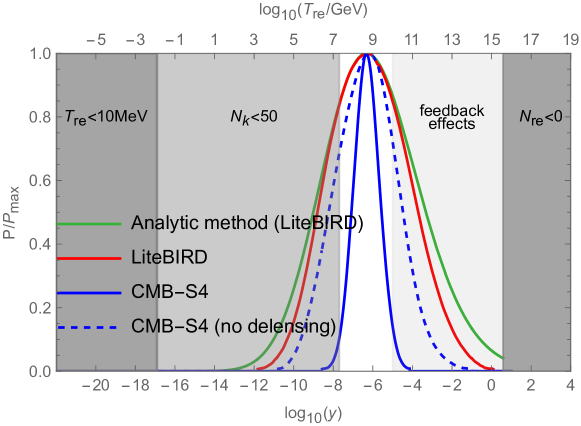
Figure 22: Here we present the posteriors for the MHI model: the green line is the result of the analytic method from Sec. 4.3 for LiteBIRD with fixed $A_{s}$. The red line is the forecast for LiteBIRD, the blue and blue-dashed lines correspond to the forecast for CMB-S4 with or without delensing, respectively (both without fixing $A_{s}$). We have not imposed the prior (52) while running the forecast, but instead indicate the region where $N_{k}<50$ in gray. When computing the sensitivities in table 5 and 4 the prior (52) was included. In the region labelled as feedback effects the conditions outlined in appendix B are not fulfilled, implying that the interpretation of the curves as posteriors for the microphysical coupling constant $y$ is questionable in this regime (while they can still be read as posteriors for $T_{\rm re}$). Here we assumed a Yukawa coupling $y$, posteriors for other types of interactions can be obtained with table 1.

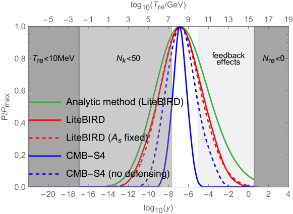
Figure 23: Posteriors for the RGI model with the same conventions as in Fig. 22. In addition to the analytic method with fixed $A_{s}$ and the forecasts with varying $A_{s}$, we also show the posterior from a LiteBIRD forecast in which $A_{s}$ was fixed (red-dashed line). This illustrates that the error bar on $A_{s}$ does not have a significant impact on the results.

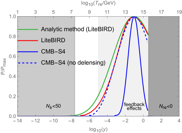
Figure 24: Posteriors for the $\alpha$-T model with the same conventions as in Fig. 22. The peak of the posterior lies in the region where feedback effects invalidate the interpretation in terms of a measurement of the microphysical coupling constant $y$, but one can still measure $T_{\rm re}$.

Finally, in Figs. 22, 23 and 24 we also compare the simple analytic method introduced in [14] and discussed in Sec. 4.3 to the forecast method introduced in Sec. 4.4 for the example of LiteBIRD. For the analytic method we therefore set $\bar{n}_{s}=0.967$, $\sigma_{n_{s}}=0.02$, $\bar{r}=$ and $\sigma_{r}$ in (55) (as in Fig. 18) while fixing $A_{s}$ to (34). As for the MCMC forecast, we choose the values of ${\rm log}_{10}{\bar{y}}$ and $\alpha$ as in Tab. 2. The resulting posteriors are the green curves in Figs. 22, 23 and 24. Comparison to the results of Sec. 4.4 shows that the two methods are overall in satisfactory agreement, proving that the simple analytic method gives reliable results when being fed with realistic estimates of $\sigma_{n_{s}}$ and $\sigma_{r}$ for given $\bar{n}_{s}$ and $\bar{r}$. For the RGI model and for the example of LiteBIRD we have also checked that fixing $A_{s}$ (as in the analytic method) would not have a significant impact on the results of the MCMC forecast: The red dashed curve in Fig. 23 shows the ${\rm log}_{10}(y)$ posterior for a forecast with $M$ (or respectively $A_{s}$) and looks almost identical to the one with $M$ being varied freely. However, as can be seen in Fig. 22, 23 and 24 the simple analytic method overestimates the confidence region of ${\rm log}_{10}(y)$ somewhat. This can be understood in the following way: In the analytic method the $n_{s}$-$r$ 2d-posterior is translated into a 1d-posterior for ${\rm log}_{10}(y)$ basically by inserting parametric expression for $n_{s}(x)$ and $r(x)$. In practice this method is therefore equivalent to treating $n_{s}$ and $r$ as free MCMC parameters while ${\rm log}_{10}(y)$ is a derived parameter. The forecasts described in Sec. 4.4 works the other way around, it assumes ${\rm log}_{10}(y)$ (and $M$ respectively) as free MCMC parameters (being the fundamental parameters of the theory) while $n_{s}$ and $r$ are derived parameters. Assuming ${\rm log}_{10}(y)$ to be the free MCMC parameter however only admits certain combinations of $n_{s}$ and $r$ values (for given $\alpha$) such that the accessible parameter space is reduced compared to the case of $n_{s}$ and $r$ as free MCMC parameters. This is ultimately reflected by a wider ${\rm log}_{10}(y)$ posterior for the analytic method.

6 Conclusion

We studied the sensitivity of LiteBIRD and CMB-S4 to cosmic reheating in three classes of inflationary models, namely RGI, MHI and $\alpha$-T models. This sensitivity is a result of the impact that the modified expansion history during the reheating epoch has on the redshifting of cosmological perturbations. In each of these classes of models we considered three fundamental parameters: The scale of inflation $M$, a parameter $\alpha$ that basically determines the relation between $M$ and the inflaton mass $m_{\phi}$, and a coupling constant $\mathsf{g}$ which controls the interaction of the inflaton with other fields. While $M$ and $\alpha$ are parameters in the effective potential $\mathcal{V}(\varphi)$ that define a model of inflation, $\mathsf{g}$ determines the efficiency of the transfer from $\varphi$ to other degrees of freedom during reheating. Gaining information on $\mathsf{g}$ probes the connection between a given model of inflation and its embedding into a more fundamental theory of particle physics. This is possible without specifying further details of the underlying particle physics model if feedback effects do not considerably modify the duration of the reheating period in a way that depends parameters other than those in the potential $\mathcal{V}(\varphi)$ and the inflaton coupling $\mathsf{g}$. We considered the four types of interactions summarised in table 1, including scalar interactions, a Yukawa interaction and and axion-like coupling.

Our work comprises two separate parts. In Sec. 3 we studied various dependencies between the fundamental parameters $\{M,\alpha,\mathsf{g}\}$ and other quantities, including the duration of inflation (characterised by $N_{k}$), the duration of reheating $N_{\rm re}$, the physical scales $\{M,m_{\phi},T_{\rm re}\}$, and the properties of CMB perturbations characterised by $\{A_{s},n_{s},r\}$. Many of these relations are given analytically in Sec. 3. We further illustrate them in the extensive set of plots given in appendix D. The main general conclusions that can be drawn from this are:

• The error bar on $n_{s}$ will remain too large to fix all three parameters $\{M,\alpha,\mathsf{g}\}$ from data alone without further model-building assumption.

• Fixing $\alpha$ defines families of inflationary models with one free parameter $M$ in the potential. In each of these families $M$ and the order of magnitude of $T_{\rm re}$ can, as a rule of thumb, be measured from a determination of $r$ at the level $\sigma_{r}\sim 10^{-3}$ if the true value of $r$ exceeds $10^{-2}$. This requires $\alpha>1$ in all models.

• This can be translated into a measurement of the order of magnitude of the inflaton coupling $\mathsf{g}$ if the values of all involved coupling constants are smaller than a critical value that can be estimated in terms of half-integer powers of $rA_{s}$ in (27).

A slightly more general discussion of point 3) is presented in appendix B. In MHI and RHI type models there is a sizeable parameter region in which these conditions can be fulfilled while being consistent with current observational data, cf. Figs. 7 and 12. In $\alpha$-T models it is more challenging, though the blue discs in Fig. 16 show that it is possible if multi-field effects can be neglected at the end of reheating.

In the second part of this work we investigated whether observations with LiteBIRD or CMB-S4 (both of which are expected to have a sensitivity around $\sigma_{r}\sim 10^{-3}$) will be able to impose meaningful constraints on the orders of magnitude of the reheating temperature and the inflaton coupling. The main result of this part are presented in Figs. 19-21 and Figs. 22-24, with the most important quantities summarised in tables 4 and 5. They were obtained by performing MCMC forecasts in which $M$ and ${\rm log}_{10}\mathsf{g}$ were treated as free MCMC parameters (along with the other parameters of the cosmological concordance model), as outlined in Sec. 4.4. The main conclusions are:

• Figs. 19-21 show that both, CMB-S4 and LiteBIRD can measure the orders of magnitudes of $M$ and $T_{\rm re}$.

• In the RGI and MHI type models this will permit to measure the order of magnitude of the inflaton coupling $\mathsf{g}$ independently of parameters other than those in the inflaton potential, as the peak of the posterior falls into the white regions in Figs. Figs. 22 and 23.

• CMB-S4 tends to perform better than LiteBIRD in all scenarios we considered. In addition to the moderately higher sensitivity to $r$, this is also related to the considerably better sensitivity to $n_{s}$. However, how large this advantage really is crucially depends on the ability to perform delensing.

• Since LiteBIRD is significantly more sensitive to $A_{s}$ while CMB-S4 is significantly more sensitive to $n_{s}$ and moderately more sensitive to $r$ (assuming successful delensing), combining data from both observations will lead to better constraints on $\mathsf{g}$.

Further improvement would be possible if additional quantities are included (e.g. the running of $n_{s}$ or non-Gaussianities), and if non-CMB data is added (e.g. from galaxy surveys and 21cm observations). Quantifying this improvement goes beyond the scope of this work and should be addressed with future studies.

Finally, we compared the analytic method summarised in Sec. 4.3 to the forecasts described in Sec. 4.4. We find that the analytic method gives rather accurate results. This is true even if $A_{s}$ is fixed, so that one practically performs an very simple one-dimensional application of Bayes formula. We illustrate this result for the RGI model in Fig. 23. The agreement between the methods is not specific to the RGI model.

• We conclude that the analytic method from Sec. 4.3 provides a very useful tool to estimate the sensitivity of future missions to the reheating temperature and the inflaton coupling, provided that information on the expected uncertainties $\sigma_{n_{s}}$ and $\sigma_{r}$ as functions of the true values of $r$ and $n_{s}$ is available.

To summarise, we studied the relations between fundamental model parameters, the physics of the reheating epoch, and CMB observables in plateau-type models of inflation. We performed the first MCMC forecasts to show that LiteBIRD and CMB-S4 can simultaneously measure the scale of inflation and the order of magnitude of the reheating temperature in a given class of models if the true value of $r$ is at least around $10^{-2}$, and assuming a standard radiation-dominated expansion history between reheating and BBN. Our results confirm earlier findings obtained with the analytic method in [14]. This would be the first ever measurement of ${\rm log}_{10}T_{\rm re}$ (in the sense that both an upper and lower bound can be obtained). For a sizeable fraction of the parameter space in the models considered here this can be translated into a measurement of the order of magnitude of the inflaton coupling. Obtaining any information on this microphysical parameter will represent an important achievement for both cosmology and particle physics, as it can provide a clue to understand how a given model of inflation can be embedded into a more fundamental theory of nature. This perspective clearly adds to the science cases for LiteBIRD and CMB-S4. It also motivates further theoretical work to investigate which observables in addition to $\{A_{s},n_{s},r\}$ can be used to constrain the inflaton coupling.

Acknowledgments

We thank J. Hamann, Y. Y. Y. Wong and for helpful discussions. We furthermore thank T. Brinckmann for his help with MontePython. MaD thanks Eiichiro Komatsu for helpful input during the early stage of this project, Antonio M. Soares for cross-checking the illustrative computation in Sec. 2.4, and Jin U Kang for many contributions to previous projects that made this line of research possible. Computational resources have been provided by the supercomputing facilities of the Université catholique de Louvain (CISM/UCL) and the Consortium des Équipements de Calcul Intensif en Fédération Wallonie Bruxelles (CÉCI) funded by the Fond de la Recherche Scientifique de Belgique (F.R.S.-FNRS) under convention 2.5020.11 and by the Walloon Region. L.M. acknowledges the State Scholarship Fund managed by the China Scholarship Council (CSC) and the Project funded by China Postdoctoral Science Foundation (2022M723677). I. M. O. acknowledges support by Fonds de la recherche scientifique (FRS-FNRS).

Appendix A Pivot scale for $r$

In this brief appendix we explicitly write out the relation between the tensor-to-scalar ratio $r$ and the also often quoted tensor-to-scalar ratio $r_{0.002}$. While the here presented derivation is essentially trivial, we believe that the relation between $r$ and $r_{0.002}$ is nevertheless sometimes a source of confusion.

The primordial spectrum for scalar perturbations is well approximated as

$$P_{s}(k)=A_{s}\left(\frac{k}{0.05\,\text{Mpc}^{-1}}\right)^{n_{s}-1},$$ (60)

where we explicitly chose $k_{p}=0.05$ Mpc^-1 as the pivot scale. This choice of $k_{p}$ is also the standard convention of e.g. the Planck [107] and BICEP [87] collaborations. Note that – by definition – $A_{s}$ is the amplitude of the primordial spectrum at the pivot scale, i.e. $P_{s}(0.05)=A_{s}$, and as such depends on the choice of the pivot scale.

The primordial spectrum of tensor perturbations can be written as

$$P_{t}(k)=A_{t}\left(\frac{k}{0.05\,\text{Mpc}^{-1}}\right)^{n_{t}}=rA_{s}\left(\frac{k}{0.05\,\text{Mpc}^{-1}}\right)^{-r/8},$$ (61)

where we applied the definition of the tensor-to-scalar ratio

$$r\equiv\frac{P_{t}(0.05)}{P_{s}(0.05)}=\frac{A_{t}}{A_{s}}$$ (62)

and the consistency relation for the tensor tilt $n_{t}=-r/8$. Just like $A_{s}$ and $A_{t}$ the tensor-to-scalar ratio depends as well on the choice of the pivot scale.

Depending on the context, occasionally also the tensor-to-scalar ratio at the pivot scale $0.002$ Mpc^-1 is referred to and defined as

$$r_{0.002}\equiv\frac{P_{t}(0.002)}{P_{s}(0.002)}.$$ (63)

Inserting eqs. (60) and (61) gives us finally the following relation between $r$ and $r_{0.002}$

$$r_{0.002}=r\left(\frac{0.002}{0.05}\right)^{-r/8-n_{s}+1}.$$ (64)

Appendix B Conditions for measuring the coupling constants

Reheating is in general a highly complicated nonequilibrium process (c.f. [115, 116]), making the computation of $\Gamma$ in terms of microphysical parameters challenging in practice. When translating (17) into a meaningful bound on any individual microphysical parameter (such as the inflaton coupling $\mathsf{g}$), one faces the problem that feedback effects introduce a dependence of $\Gamma$ on a large sub-set of the parameters $\{\mathsf{a}_{i}\}$ in the underlying particle physics theory. Rather than being a mere problem of limited computational power, this is actually a fundamental restriction, as the dependence on the $\{\mathsf{a}_{i}\}$ makes it impossible to determine $\mathsf{g}$ from the CMB without having to specify the details of the underlying particle physics model. It is, however, possible if reheating proceeds sufficiently slowly that feedback effects can be neglected. The conditions for this have been studies in detail in [13], here we only quote the results. The dominant source of $\{\mathsf{a}_{i}\}$-dependence lies in the explosive resonant particle production due to non-perturbative effects, sometimes referred to as preheating. In addition to that there are also thermal corrections to the elementary decay rate (18), which bring in a dependence on the $\{\mathsf{a}_{i}\}$ (e.g. through the thermal masses of the decay products), cf. table 6. Preheating leads to very large occupation numbers for the produced particles, and the interactions of $\varphi$ with the produced particles affect the effective $\Gamma$. This introduces a dependence of $\Gamma$ on the properties of the produced particles, and hence the $\{\mathsf{a}_{i}\}$. There are two different types of conditions to ensure that such feedback effects do not modify $N_{\rm re}$.

interaction	process	contribution to $\Gamma$
$g\Phi\chi^{2}$	$\varphi\to\chi\chi$	$\frac{g^{2}}{8\pi M_{\phi}}\big{(}1-2M_{\chi}/M_{\phi}\big{)}^{1/2}\big{(}1+2f_{B}(M_{\phi}/2)\big{)}\theta(M_{\phi}-2M_{\chi})$	[117]
$\frac{\kappa}{4}\Phi^{2}\chi^{2}$	$\varphi\varphi\to\chi\chi$	$\frac{h^{2}\varphi^{2}}{256\pi M_{\phi}}\big{(}1-M_{\chi}/M_{\phi}\big{)}^{1/2}\big{(}1+2f_{B}(M_{\phi})\big{)}\theta(M_{\phi}-M_{\chi})$	[118]
$\frac{\sigma}{\Lambda}\Phi F_{\mu\nu}\tilde{F}^{\mu\nu}$	$\varphi\to\gamma\gamma$	$\frac{\sigma^{2}}{4\pi}\frac{M_{\phi}^{3}}{\Lambda^{2}}\big{(}1-2M_{\gamma}/M_{\phi}\big{)}^{1/2}\big{(}1+2f_{B}(M_{\phi}/2)\big{)}\theta(M_{\phi}-2M_{\gamma})$	[119]
$y\Phi\bar{\psi}\psi$	$\varphi\to\psi\bar{\psi}$, ${\color[rgb]{0,0,0}M_{\psi}\simeq m_{\psi}}$	$\frac{y^{2}}{8\pi}M_{\phi}\big{(}1-2m_{\psi}/M_{\phi}\big{)}^{3/2}\big{(}1-2f_{F}(M_{\phi}/2)\big{)}\theta(M_{\phi}-2m_{\psi})$	[120]
	$\varphi\to\psi\bar{\psi}$, $M_{\psi}\gg m_{\psi}$	$\frac{y^{2}}{8\pi}M_{\phi}\big{(}1-2M_{\psi}/M_{\phi}\big{)}^{1/2}\big{(}1-2f_{F}(M_{\phi}/2)\big{)}\theta(M_{\phi}-2M_{\psi})$	[120]

.

Table 6: Contributions to $\Gamma$ from different elementary processes mediated by some of the interactions in table 1 in a thermal plasma at temperature $T$ that were considered in [13], cf. (19). Small letters and capital letters denote vacuum masses and effective thermal masses, respectively. In practice the quantum-statistical corrections involving the Bose-Einstein and Fermi-Dirac distributions and $f_{F}(\omega)=(e^{\omega/T}+1)^{-1}$ and $f_{B}(\omega)=(e^{\omega/T}-1)^{-1}$ can be neglected, as $T\ll M_{\phi}$ in the regime where (66) and (68) are fulfilled, so that the use of (18) is justified. This simplifies the analysis, as one can easily convert the constraints on one coupling $\mathsf{g}$ in constraints in any of the others with table 1. The interaction with $\kappa$ (which leads to non-linearites that can limit the validity of (1) [121]) cannot effectively reheat the universe in the regime where the condition (68) is fulfilled. Thermal corrections to the $h\Phi\chi^{3}/3!$ interaction have been considered in [120, 122], but no closed analytic form is known. For the other interactions it is easy to see that the $T\to 0$ limit reproduces the rate in table 1.

Conditions on the inflaton potential.

The first type concerns the inflaton self-interactions $\{\mathsf{v}_{i}\}$ and thereby restricts the choice of the model of inflation (specified by a choice of $\{\mathsf{v}_{i}\}$). For the models considered here the minimum of $\mathcal{V}(\varphi)$ is at $\varphi=0$, so that we can Taylor expand

$$\mathcal{V}(\varphi)=\sum_{j}\frac{\mathsf{v}_{j}}{j!}\frac{\varphi^{j}}{\Lambda^{j-4}}$$ (65)

with $\mathsf{v}_{3}=g_{\phi}/3!$, $\mathsf{v}_{4}=\lambda_{\phi}/4!$ in (20) etc. If one neglects radiative corrections, the coefficients in this expansion can be identified with the inflaton mass and coupling constants of the self-interactions in the expansion of the potential $V(\Phi)$ in the Lagrangian. The inflaton self-interactions can in general lead to parametric or tachyonic resonances that reheat the universe well before elementary decays become relevant, invalidating the use of (18) in (17), and introducing a dependence on the $\{\mathsf{a}_{i}\}$. This can be avoided if [13]

$$|\mathsf{v}_{j}|\ll\left(\frac{\omega}{\varphi}\right)^{j-\frac{5}{2}}{\rm min}\left(\sqrt{\frac{\omega}{M_{pl}}},\sqrt{\frac{\omega}{\varphi}}\right)\ \left(\frac{\omega}{\Lambda}\right)^{4-j},$$ (66)

with $\omega$ the frequency of the inflaton oscillations. This practically restricts us to approximately parabolic potentials in which the oscillating inflaton has a matter-like equation of state (25). Leaving aside sub-dominant non-linear corrections to the equation of motion (1), the frequency of these oscillations is given by the effective in-medium inflaton mass $\omega\simeq M_{\phi}$. In principle $M_{\phi}$ depends on not only on the couplings to other particles $\{\mathsf{g}_{i}\}$, but also on their interactions with each other, and hence on the $\{\mathsf{a}_{i}\}$. However, (66) imposes the strongest constraint when $\varphi$ is maximal, i.e., at the beginning of the reheating phase, and we can replace $\varphi\to\varphi_{\rm end}$ in (66) to obtain a conservative bound. At that moment the universe is empty. Hence, the frequency of the inflaton oscillations is in good approximation given by its vacuum mass $\omega\simeq m_{\phi}$.

Conditions on the couplings to other fields.

Consider an interaction term of the form

$$\mathsf{g}\Phi^{j}\Lambda^{4-D}\mathcal{O}[\{\mathcal{X}_{i}\}],$$ (67)

where $\mathcal{O}[\{\mathcal{X}_{i}\}]$ is an operator of mass dimension $D-j$ that is composed of fields $\mathcal{X}_{i}$ other than $\Phi$, and $\mathsf{g}$ a dimensionless coupling constant. For $D>4$ the scale $\Lambda$ marks the cutoff of an effective field theory description in which (67) appears, and we assume that it exceeds all other relevant scales for this effective description to be valid. For $D<4$ we set $\Lambda=m_{\phi}$ for convenience, in this case $\Lambda$ is simply introduced to make $\mathsf{g}$ dimensionless and has no physical meaning. A term of the form (67) introduces a time-varying effective mass $\propto\mathsf{g}\varphi^{j}$ for a field $\mathcal{X}$ at tree level if $\mathcal{O}[\{\mathcal{X}_{i}\}]$ is a bilinear in $\mathcal{X}$. Some examples of this kind are given in table 1. For bosonic $\mathcal{X}$ this implies $D=j+2$, for fermionic $\mathcal{X}$ it implies $D=j+3$. It is generally justified to evaluate the LHS in (17) with (18) if [13]

$$|\mathsf{g}|\ll\left(\frac{m_{\phi}}{\varphi_{\rm end}}\right)^{j-\frac{1}{2}}{\rm min}\left(\sqrt{\frac{m_{\phi}}{M_{pl}}},\sqrt{\frac{m_{\phi}}{\varphi_{\rm end}}}\right)\ \left(\frac{m_{\phi}}{\Lambda}\right)^{4-D}.\$$ (68)

The condition (68) imposes a strong upper bound on interactions that are non-linear in $\Phi$. For terms with $D>4$ the smallness of $(m_{\phi}/\varphi_{\rm end})^{j-\frac{1}{2}}$ can be alleviated by the fact that $m_{\phi}/\Lambda\ll 1$, but e.g. represents a strong restriction on interactions of the type $\frac{\kappa}{4}\Phi^{2}\chi^{2}$. This is the reason why we have focused on operators with $j=1$ in table 1.

Keeping in mind that the requirement (24) of avoiding self-resonances during reheating restricts us to potentials that are roughly parabolic at the end of inflation, the inflaton mass $m_{\phi}$ is typically suppressed with respect to $M_{pl}$ as $m_{\phi}\sim M^{2}/\varphi_{\rm end}$, with $M$ the typical energy scale during inflation. This follows from $\mathcal{V}(\varphi_{\rm end})\simeq\frac{1}{2}m_{\phi}^{2}\varphi_{\rm end}^{2}\sim\mathcal{V}(\varphi_{k})\sim M^{4}$, where the second relation assumed that $\mathcal{V}(\varphi_{\rm end})$ is of the same order of magnitude as $\mathcal{V}(\varphi_{k})$ due to the flatness of the potential during inflation. Using (7) one then finds

$$m_{\phi}\sim\frac{M_{pl}^{2}}{\varphi_{\rm end}}\pi\sqrt{3rA_{s}}\ ,\quad M\sim M_{pl}\left(\frac{3\pi^{2}}{2}A_{s}r\right)^{1/4}$$ (69)

Focusing on renormalisable couplings and assuming $\phi_{\rm end}\simeq M_{pl}$ one finds a simple estimate (27) for (68),

$$|\mathsf{v}_{j}|\ll\left(3\pi^{2}rA_{s}\right)^{(j-2)/2}\ ,\ |\mathsf{g}|\ll\left(3\pi^{2}rA_{s}\right)^{j/2}$$

Plugging in the upper bound $r=0.06$ from [86] yields an upper bound of $4\times 10^{-5}$ on $\mathsf{g}$ for interactions that are linear in $\Phi$, which is larger than the electron Yukawa coupling in the Standard Model of particle physics. In the derivation of (27) we neglected various numerical prefactors that depend on the parameters $\{\mathsf{v}_{i}\}$ in the potential, which limits its applicability to rough estimates. It is nevertheless a very useful criterion due to its remarkable simplicity, and it provides an explanation for the otherwise surprisingly similar numerical values that the upper bound (68) yields when applied to the different models. Finally, we can use the estimate of $M$ in (69) to rewrite (27) as

$$|\mathsf{v}_{j}|\ll\left(M/M_{pl}\right)^{2(j-2)}\ ,\ |\mathsf{g}|\ll\left(M/M_{pl}\right)^{2j}$$ (70)

implying that models with a comparably low energy scale of inflation can avoid a parametric resonance only for very small values of the inflaton coupling.

Effects that can relax the conditions.

The conditions (66) and (68) impose very strong constraints on interactions that are not linear in $\Phi$, i.e., with $j>1$. Luckily it turns out that the relations (68) and (66) from which it is derived are too conservative in most realistic models. They guarantee the absence of feedback effects without relying on any further assumptions about the underlying particle physics model (solely due to redshifting of the produced particles). In reality there are a number of mechanisms that suppress feedback which in principle rely on assumptions about the particle physics embedding, but in practice occur quite generically. One of them is the decay of the produced particles. The interaction (67) generates a time-dependent contribution $\propto\mathsf{g}\varphi^{j}\Lambda^{4-D}$ to the squared effective mass of the particles $\mathcal{X}$ that couple to $\Phi$. This causes non-perturbative particle production during the zero-crossings of $\varphi$, which can trigger a parametric or tachyonic resonance that quickly reheats the universe if condition (68) is violated. However, the same term makes the produced $\mathcal{X}$-particles very heavy when the elongation of $\varphi$ is maximal, implying that they are very short-lived and can decay between two zero-crossings, which can considerably delay or even avoid the resonant particle production, cf. e.g. [124]. Another effect is the screening of particles into quasiparticles with effective in-medium masses $M_{\mathcal{X}}$ once the universe is filled with radiation. This terminates the resonant particle production as soon as $M_{\mathcal{X}}^{2}\sim\mathsf{g}\varphi^{j}\Lambda^{4-D}$, which can happen well before the radiation dominates the total energy of the universe.

For instance, consider the $h\phi^{2}\chi^{2}/4$ interaction in table 1 and add a $\lambda_{\chi}\chi^{4}/4!$ self-interaction, which generates a thermal mass $M_{\chi}^{2}\simeq\lambda_{\chi}T^{2}/24$. The thermal mass terminates the resonant non-pertrubative particle production for $M_{\chi}^{2}\sim h\varphi^{2}/2$, which happens at a temperature $T\sim\varphi\sqrt{12h/\lambda_{\chi}}$. The ratio between radiation density and $\mathcal{V}$ is given by $\frac{\pi^{2}g_{*}}{15}\frac{T^{4}}{m_{\phi}^{2}\varphi^{2}}\simeq\frac{48\pi^{4}g_{*}}{5}(h/\lambda_{\chi})^{2}(\varphi/m_{\phi})^{2}$. Radiation is sub-dominant at the moment when the resonance is terminated if $h/\lambda_{\chi}<m_{\phi}/(30\sqrt{g_{*}}\varphi)$. This condition is parametrically much weaker than (68), as it basically requires $h\ll m_{\phi}/\varphi$, while (68) requires $h\ll(m_{\phi}/\varphi)^{2}$. It becomes even weaker if $\chi$-decays have delayed the resonance so that $\varphi<\varphi_{\rm end}$. For the $g\Phi\chi^{2}$ interaction analogous considerations lead to the condition $g\ll\lambda_{\chi}$. The assumption that the $\chi$-particles have thermalised does not appear to be crucial, as similar results have been obtained in [123] without that assumption, confirming that effective masses can easily terminate the resonant particle production before it has converted the inflaton energy into radiation.

Hence, even if the inflaton couplings violate the conditions (68) and feedback effects strongly affect the rate of particle production in the initial phase of (p)reheating, elementary decays may still account for most of ther energy transfer from $\varphi$ into radiation. In this case we can still use (18) in (17) to obtain a constraint on $\mathsf{g}$. The reason is that feedback effects only introduce a $\{\mathsf{a}_{i}\}$-dependence in the CMB observables if they modify the duration of reheating i.e., the expansion history of the universe. This happens if $\Gamma$ depends on the $\{\mathsf{a}_{i}\}$ at the moment when it equals $H$, cf. (17).

Appendix C Revisiting $\alpha$-attractor $E$ models

The $\alpha$-attractor models of the $E$-type [125, 126, 20, 21] are characterised by the potential

$$\mathcal{V}(\varphi)=M^{4}\left(1-e^{-\sqrt{\frac{2}{3\alpha}}\frac{\varphi}{M_{pl}}}\right)^{2n}.$$ (71)

Solving (2) for the condition that $\epsilon=1$ we find

$$\varphi_{\rm end}=\sqrt{\frac{3\alpha}{2}}M_{pl}{\rm ln}\left(\frac{2n}{\sqrt{3\alpha}}+1\right).$$ (72)

From (6) we further find

$$\varphi_{k}=\sqrt{\frac{3\alpha}{2}}M_{pl}{\rm ln}\left(\frac{8n}{\sqrt{3r\alpha}}+1\right)$$ (73)

In order to ensure that $\mathcal{V}(\varphi)$ is parabolic near the minimum we require that $n=1$, leading to a Starobinsky-like potential [2]. Taylor expansion yields

$$m_{\phi}^{2}=\frac{4M^{4}}{3M_{pl}^{2}\alpha}\ ,\ g_{\phi}=\frac{2M^{4}}{3M_{pl}^{3}}\sqrt{\frac{2}{3\alpha^{3}}}\ ,\ \frac{\lambda_{\phi}}{4!}=\frac{7}{27\alpha^{2}}\frac{M^{4}}{M_{pl}^{4}}.$$ (74)

Plugging (74) into (26) we find that indeed the quadratic term dominates over the cubic and quartic at the end of inflation for any $\alpha\geq 1$. However, condition (24) is violated for practically all values of $\alpha$ used in [40, 43, 48] (and likely all values of $\alpha$ that can be made consistent with the current observational bound on $r$), invalidating the extraction of the inflaton coupling $\mathsf{g}$ from CMB data (while the determination of the effective $T_{\rm re}$ remains valid). Note, however, that this conclusion may be too conservative, as already stated in Sec. B. The more detailed analysis in [127] suggests that a self-resonance may still be avoided for values of $\alpha$ or order unity.

Before closing we remark that Fig. 3 in [43], which describes the $n_{s}$-dependence of $N_{\rm re}$ and $T_{\rm re}$ in the $\alpha$-attractor E-model with $n=1$ for various values of $\alpha$, needs minor modifications. When $n_{s}$ is fixed, the value of $N_{\rm re}$ and $T_{\rm re}$ do not change monotonically in the parameter range $1\leq\alpha\leq 100$, as can be seen in Fig. 25. This effect also exists in the mutated hilltop model discussed in section 3.1.

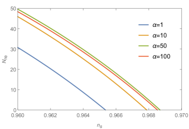
(a)

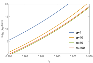
(b)

Figure 25: Corrected version of Fig. 3 in [43], describing the $n_{s}$-dependence of $N_{\rm re}$ and $T_{\rm re}$ in the $\alpha$-attractor E-model with $n=1$ for various values of $\alpha$.

Appendix D Illustrative plots for various parameter choices

In this appendix we show the dependence of $T_{\rm re}$, $N_{k}$, $N_{\rm re}$ and the inflaton coupling constants $\mathsf{g}$ on various parameters in the models considered in this work. We consider a broader range of choices for $\alpha$, but keep $A_{s}$ fixed to (34).

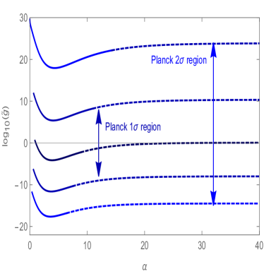
(a)

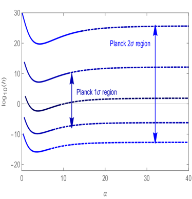
(b)

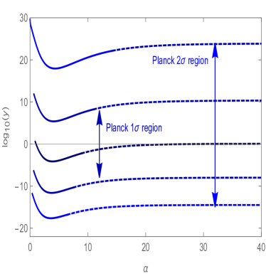
(c)

(d)

Figure 26: The relation between the inflaton couplings and $\alpha$ in the MHI model for different choices of $n_{s}$, with conventions as in Fig. 4.

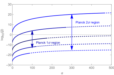
(a)

(b)

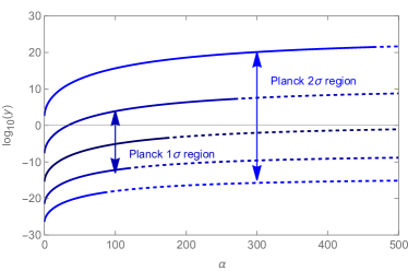
(c)

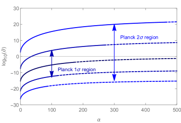
(d)

Figure 32: The relation between the inflaton couplings and $\alpha$ in the RGI model for different choices of $n_{s}$, with conventions as in Fig. 4.

(a)

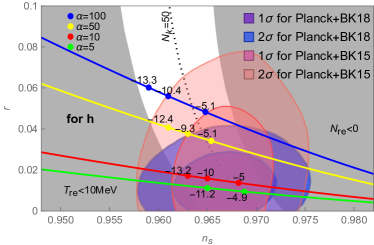
(b)

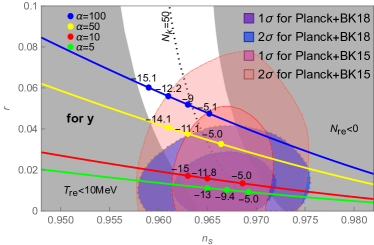
(c)

(d)

Figure 33: Impact of the reheating phase on the predictions of RGI model for $n_{s}$ and $r$ for a set of sample points. The notations are the same with Fig 7.

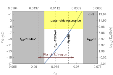
(a)

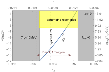
(b)

(c)

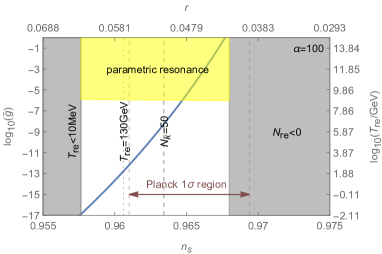
(d)

Figure 34: Dependence of the scalar coupling $\tilde{g}$ on $n_{s}$ in the RGI model for different choices of $\alpha$. The notations are the same with Fig. 8.

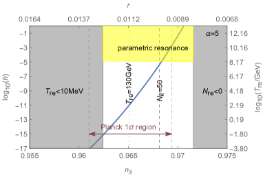
(a)

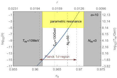
(b)

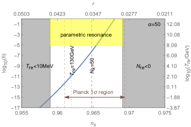
(c)

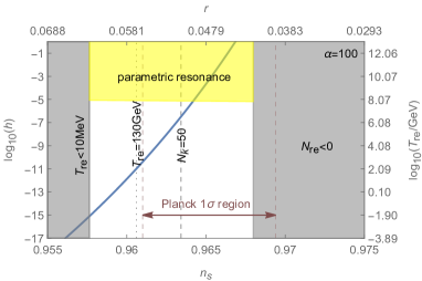
(d)

Figure 35: Dependence of the scalar coupling $h$ on $n_{s}$ in the RGI model for different choices of $\alpha$. The notations are the same with Fig. 8.

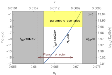
(a)

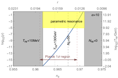
(b)

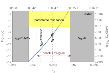
(c)

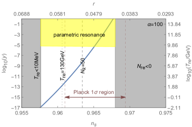
(d)

Figure 36: Dependence of the Yukawa coupling $y$ on $n_{s}$ in the RGI model for different choices of $\alpha$. The notations are the same with Fig. 8.

(a)

(b)

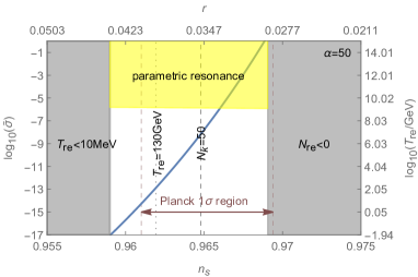
(c)

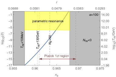
(d)

Figure 37: Dependence of the axion-like coupling $\tilde{\sigma}$ on $n_{s}$ in the RGI model for different choices of $\alpha$. The notations are the same with Fig. 8.

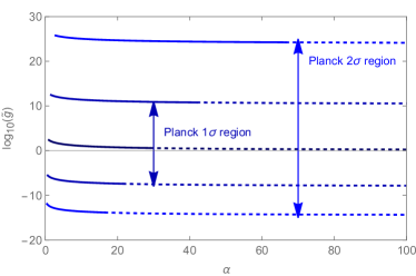
(a)

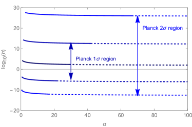
(b)

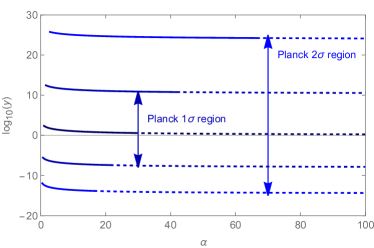
(c)

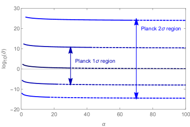
(d)

Figure 38: The relation between the inflaton couplings and $\alpha$ in the $\alpha$-T model for different choices of $n_{s}$, with conventions as in Fig. 4.

(a)

(b)

(c)

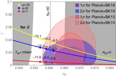
(d)

Figure 39: Impact of the reheating phase on the predictions of $\alpha$-T model for $n_{s}$ and $r$ for a set of sample points. The notations are the same with Fig. 7.

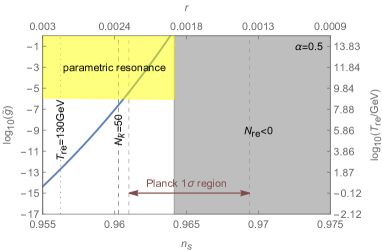
(a)

(b)

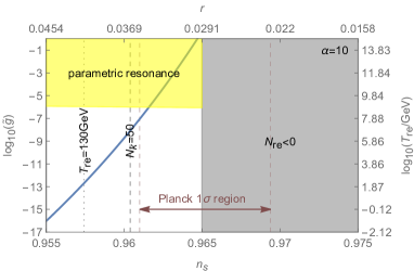
(c)

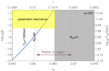
(d)

Figure 40: Dependence of the scalar coupling $\tilde{g}$ on $n_{s}$ in the $\alpha$-T model for different choices of $\alpha$. The notations are the same with Fig. 8.

(a)

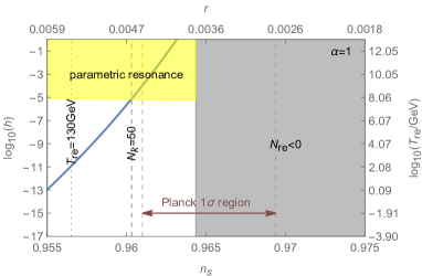
(b)

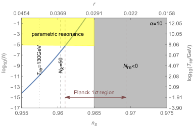
(c)

(d)

Figure 41: Dependence of the scalar coupling $h$ on $n_{s}$ in the $\alpha$-T model for different choices of $\alpha$. The notations are the same with Fig. 8.

(a)

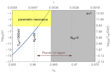
(b)

(c)

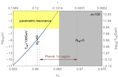
(d)

Figure 42: Dependence of the Yukawa coupling $y$ on $n_{s}$ in the $\alpha$-T model for different choices of $\alpha$. The notations are the same with Fig. 8.

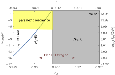
(a)

(b)

(c)

(d)

Figure 43: Dependence of the axion-like coupling $\tilde{\sigma}$ on $n_{s}$ in the $\alpha$-T model for different choices of $\alpha$. The notations are the same with Fig. 8.

References

- [1] A.A. Starobinsky, Spectrum of relict gravitational radiation and the early state of the universe, JETP Lett. 30 (1979) 682.
- [2] A.A. Starobinsky, A New Type of Isotropic Cosmological Models Without Singularity, Phys. Lett. B 91 (1980) 99.
- [3] A.H. Guth, The Inflationary Universe: A Possible Solution to the Horizon and Flatness Problems, Phys. Rev. D 23 (1981) 347.
- [4] A.D. Linde, A New Inflationary Universe Scenario: A Possible Solution of the Horizon, Flatness, Homogeneity, Isotropy and Primordial Monopole Problems, Phys. Lett. B 108 (1982) 389.
- [5] L. Moncelsi et al., Receiver development for BICEP Array, a next-generation CMB polarimeter at the South Pole, Proc. SPIE Int. Soc. Opt. Eng. 11453 (2020) 1145314 [2012.04047].
- [6] Simons Observatory collaboration, The Simons Observatory: Science goals and forecasts, JCAP 02 (2019) 056 [1808.07445].
- [7] H. Sugai et al., Updated Design of the CMB Polarization Experiment Satellite LiteBIRD, J. Low. Temp. Phys. 199 (2020) 1107 [2001.01724].
- [8] CMB-S4 collaboration, CMB-S4: Forecasting Constraints on Primordial Gravitational Waves, Astrophys. J. 926 (2022) 54 [2008.12619].
- [9] J. Martin, C. Ringeval and V. Vennin, How Well Can Future CMB Missions Constrain Cosmic Inflation?, JCAP 10 (2014) 038 [1407.4034].
- [10] J. Martin and C. Ringeval, First CMB Constraints on the Inflationary Reheating Temperature, Phys. Rev. D 82 (2010) 023511 [1004.5525].
- [11] P. Adshead, R. Easther, J. Pritchard and A. Loeb, Inflation and the Scale Dependent Spectral Index: Prospects and Strategies, JCAP 02 (2011) 021 [1007.3748].
- [12] R. Easther and H.V. Peiris, Bayesian Analysis of Inflation II: Model Selection and Constraints on Reheating, Phys. Rev. D 85 (2012) 103533 [1112.0326].
- [13] M. Drewes, Measuring the inflaton coupling in the CMB, JCAP 09 (2022) 069 [1903.09599].
- [14] M. Drewes and L. Ming, Connecting Cosmic Inflation to Particle Physics with LiteBIRD, CMB S4, EUCLID and SKA, 2208.07609.
- [15] B.K. Pal, S. Pal and B. Basu, Mutated Hilltop Inflation : A Natural Choice for Early Universe, JCAP 01 (2010) 029 [0908.2302].
- [16] B. Kumar Pal, Mutated hilltop inflation revisited, Eur. Phys. J. C 78 (2018) 358 [1711.00833].
- [17] M. Fairbairn, L. Lopez Honorez and M.H.G. Tytgat, Radion assisted gauge inflation, Phys. Rev. D 67 (2003) 101302 [hep-ph/0302160].
- [18] J. Martin, C. Ringeval, R. Trotta and V. Vennin, The Best Inflationary Models After Planck, JCAP 03 (2014) 039 [1312.3529].
- [19] R. Kallosh and A. Linde, Non-minimal Inflationary Attractors, JCAP 10 (2013) 033 [1307.7938].
- [20] J.J.M. Carrasco, R. Kallosh and A. Linde, -Attractors: Planck, LHC and Dark Energy, JHEP 10 (2015) 147 [1506.01708].
- [21] J.J.M. Carrasco, R. Kallosh and A. Linde, Cosmological Attractors and Initial Conditions for Inflation, Phys. Rev. D 92 (2015) 063519 [1506.00936].
- [22] B. Audren, J. Lesgourgues, K. Benabed and S. Prunet, Conservative Constraints on Early Cosmology: an illustration of the Monte Python cosmological parameter inference code, JCAP 02 (2013) 001 [1210.7183].
- [23] T. Brinckmann and J. Lesgourgues, MontePython 3: boosted MCMC sampler and other features, Phys. Dark Univ. 24 (2019) 100260 [1804.07261].
- [24] G.F. Giudice, E.W. Kolb and A. Riotto, Largest temperature of the radiation era and its cosmological implications, Phys. Rev. D 64 (2001) 023508 [hep-ph/0005123].
- [25] F.L. Bezrukov and M. Shaposhnikov, The Standard Model Higgs boson as the inflaton, Phys. Lett. B 659 (2008) 703 [0710.3755].
- [26] A. Albrecht, P.J. Steinhardt, M.S. Turner and F. Wilczek, Reheating an Inflationary Universe, Phys. Rev. Lett. 48 (1982) 1437.
- [27] A.D. Dolgov and D.P. Kirilova, ON PARTICLE CREATION BY A TIME DEPENDENT SCALAR FIELD, Sov. J. Nucl. Phys. 51 (1990) 172.
- [28] J.H. Traschen and R.H. Brandenberger, Particle Production During Out-of-equilibrium Phase Transitions, Phys. Rev. D 42 (1990) 2491.
- [29] Y. Shtanov, J.H. Traschen and R.H. Brandenberger, Universe reheating after inflation, Phys. Rev. D 51 (1995) 5438 [hep-ph/9407247].
- [30] L. Kofman, A.D. Linde and A.A. Starobinsky, Reheating after inflation, Phys. Rev. Lett. 73 (1994) 3195 [hep-th/9405187].
- [31] D. Boyanovsky, H.J. de Vega, R. Holman and J.F.J. Salgado, Analytic and numerical study of preheating dynamics, Phys. Rev. D 54 (1996) 7570 [hep-ph/9608205].
- [32] L. Kofman, A.D. Linde and A.A. Starobinsky, Towards the theory of reheating after inflation, Phys. Rev. D 56 (1997) 3258 [hep-ph/9704452].
- [33] J. Cooley et al., Report of the Topical Group on Particle Dark Matter for Snowmass 2021, 2209.07426.
- [34] L. Canetti, M. Drewes and M. Shaposhnikov, Matter and Antimatter in the Universe, New J. Phys. 14 (2012) 095012 [1204.4186].
- [35] C. Caprini and D.G. Figueroa, Cosmological Backgrounds of Gravitational Waves, Class. Quant. Grav. 35 (2018) 163001 [1801.04268].
- [36] J. Ghiglieri and M. Laine, Gravitational wave background from Standard Model physics: Qualitative features, JCAP 07 (2015) 022 [1504.02569].
- [37] J. Ghiglieri, G. Jackson, M. Laine and Y. Zhu, Gravitational wave background from Standard Model physics: Complete leading order, JHEP 07 (2020) 092 [2004.11392].
- [38] A. Ringwald, J. Schütte-Engel and C. Tamarit, Gravitational Waves as a Big Bang Thermometer, JCAP 03 (2021) 054 [2011.04731].
- [39] J.L. Cook, E. Dimastrogiovanni, D.A. Easson and L.M. Krauss, Reheating predictions in single field inflation, JCAP 04 (2015) 047 [1502.04673].
- [40] Y. Ueno and K. Yamamoto, Constraints on -attractor inflation and reheating, Phys. Rev. D 93 (2016) 083524 [1602.07427].
- [41] K. Nozari and N. Rashidi, Perturbation, non-Gaussianity, and reheating in a Gauss-Bonnet -attractor model, Phys. Rev. D 95 (2017) 123518 [1705.02617].
- [42] A. Di Marco, P. Cabella and N. Vittorio, Constraining the general reheating phase in the -attractor inflationary cosmology, Phys. Rev. D 95 (2017) 103502 [1705.04622].
- [43] M. Drewes, J.U. Kang and U.R. Mun, CMB constraints on the inflaton couplings and reheating temperature in -attractor inflation, JHEP 11 (2017) 072 [1708.01197].
- [44] D. Maity and P. Saha, Connecting CMB anisotropy and cold dark matter phenomenology via reheating, Phys. Rev. D 98 (2018) 103525 [1801.03059].
- [45] N. Rashidi and K. Nozari, -Attractor and reheating in a model with noncanonical scalar fields, Int. J. Mod. Phys. D 27 (2018) 1850076 [1802.09185].
- [46] G. German, Constraining -attractor models from reheating, Int. J. Mod. Phys. D 31 (2022) 2250081 [2010.09795].
- [47] S.S. Mishra, V. Sahni and A.A. Starobinsky, Curing inflationary degeneracies using reheating predictions and relic gravitational waves, JCAP 05 (2021) 075 [2101.00271].
- [48] J. Ellis, M.A.G. Garcia, D.V. Nanopoulos, K.A. Olive and S. Verner, BICEP/Keck constraints on attractor models of inflation and reheating, Phys. Rev. D 105 (2022) 043504 [2112.04466].
- [49] R.-G. Cai, Z.-K. Guo and S.-J. Wang, Reheating phase diagram for single-field slow-roll inflationary models, Phys. Rev. D 92 (2015) 063506 [1501.07743].
- [50] A. Di Marco, G. Pradisi and P. Cabella, Inflationary scale, reheating scale, and pre-BBN cosmology with scalar fields, Phys. Rev. D 98 (2018) 123511 [1807.05916].
- [51] D. Maity and P. Saha, (P)reheating after minimal Plateau Inflation and constraints from CMB, JCAP 07 (2019) 018 [1811.11173].
- [52] D. Maity and P. Saha, Minimal plateau inflationary cosmologies and constraints from reheating, Class. Quant. Grav. 36 (2019) 045010 [1902.01895].
- [53] S. Antusch, D.G. Figueroa, K. Marschall and F. Torrenti, Energy distribution and equation of state of the early Universe: matching the end of inflation and the onset of radiation domination, Phys. Lett. B 811 (2020) 135888 [2005.07563].
- [54] L. Dai, M. Kamionkowski and J. Wang, Reheating constraints to inflationary models, Phys. Rev. Lett. 113 (2014) 041302 [1404.6704].
- [55] V. Domcke and J. Heisig, Constraints on the reheating temperature from sizable tensor modes, Phys. Rev. D 92 (2015) 103515 [1504.00345].
- [56] I. Dalianis, G. Koutsoumbas, K. Ntrekis and E. Papantonopoulos, Reheating predictions in Gravity Theories with Derivative Coupling, JCAP 02 (2017) 027 [1608.04543].
- [57] J.B. Munoz and M. Kamionkowski, Equation-of-State Parameter for Reheating, Phys. Rev. D 91 (2015) 043521 [1412.0656].
- [58] N. Zhang, Y.-B. Wu, J.-W. Lu, C.-W. Sun, L.-J. Shou and H.-Z. Xu, Constraints on the generalized natural inflation after Planck 2018, Chin. Phys. C 44 (2020) 095107 [1807.03596].
- [59] N.K. Stein and W.H. Kinney, Natural inflation after Planck 2018, JCAP 01 (2022) 022 [2106.02089].
- [60] J.-O. Gong, S. Pi and G. Leung, Probing reheating with primordial spectrum, JCAP 05 (2015) 027 [1501.03604].
- [61] R.J. Hardwick, V. Vennin, K. Koyama and D. Wands, Constraining Curvatonic Reheating, JCAP 08 (2016) 042 [1606.01223].
- [62] S.-M. Choi and H.M. Lee, Inflection point inflation and reheating, Eur. Phys. J. C 76 (2016) 303 [1601.05979].
- [63] F. Takahashi and W. Yin, ALP inflation and Big Bang on Earth, JHEP 07 (2019) 095 [1903.00462].
- [64] P. Cabella, A. Di Marco and G. Pradisi, Fiber inflation and reheating, Phys. Rev. D 95 (2017) 123528 [1704.03209].
- [65] A. Nautiyal, Reheating constraints on Tachyon Inflation, Phys. Rev. D 98 (2018) 103531 [1806.03081].
- [66] R. Kabir, A. Mukherjee and D. Lohiya, Reheating constraints on Kähler moduli inflation, Mod. Phys. Lett. A 34 (2019) 1950114 [1609.09243].
- [67] S. Bhattacharya, K. Dutta and A. Maharana, Constraints on Kähler moduli inflation from reheating, Phys. Rev. D 96 (2017) 083522 [1707.07924].
- [68] I. Dalianis and Y. Watanabe, Probing the BSM physics with CMB precision cosmology: an application to supersymmetry, JHEP 02 (2018) 118 [1801.05736].
- [69] M. Drewes, What can the CMB tell about the microphysics of cosmic reheating?, JCAP 03 (2016) 013 [1511.03280].
- [70] S. Renaux-Petel and K. Turzyński, Geometrical Destabilization of Inflation, Phys. Rev. Lett. 117 (2016) 141301 [1510.01281].
- [71] Y. Ema, R. Jinno, K. Mukaida and K. Nakayama, Violent Preheating in Inflation with Nonminimal Coupling, JCAP 02 (2017) 045 [1609.05209].
- [72] E.I. Sfakianakis and J. van de Vis, Preheating after Higgs Inflation: Self-Resonance and Gauge boson production, Phys. Rev. D 99 (2019) 083519 [1810.01304].
- [73] T. Krajewski, K. Turzyński and M. Wieczorek, On preheating in -attractor models of inflation, Eur. Phys. J. C 79 (2019) 654 [1801.01786].
- [74] O. Iarygina, E.I. Sfakianakis, D.-G. Wang and A. Achucarro, Universality and scaling in multi-field -attractor preheating, JCAP 06 (2019) 027 [1810.02804].
- [75] O. Iarygina, E.I. Sfakianakis, D.-G. Wang and A. Achúcarro, Multi-field inflation and preheating in asymmetric -attractors, 2005.00528.
- [76] LiteBIRD collaboration, Probing Cosmic Inflation with the LiteBIRD Cosmic Microwave Background Polarization Survey, 2202.02773.
- [77] A. Achúcarro et al., Inflation: Theory and Observations, 2203.08128.
- [78] E. Komatsu, New physics from the polarized light of the cosmic microwave background, Nature Rev. Phys. 4 (2022) 452 [2202.13919].
- [79] Y. Mao, M. Tegmark, M. McQuinn, M. Zaldarriaga and O. Zahn, How accurately can 21 cm tomography constrain cosmology?, Phys. Rev. D 78 (2008) 023529 [0802.1710].
- [80] K. Kohri, Y. Oyama, T. Sekiguchi and T. Takahashi, Precise Measurements of Primordial Power Spectrum with 21 cm Fluctuations, JCAP 10 (2013) 065 [1303.1688].
- [81] J.B. Muñoz, E.D. Kovetz, A. Raccanelli, M. Kamionkowski and J. Silk, Towards a measurement of the spectral runnings, JCAP 05 (2017) 032 [1611.05883].
- [82] J. Martin, C. Ringeval and V. Vennin, Information Gain on Reheating: the One Bit Milestone, Phys. Rev. D 93 (2016) 103532 [1603.02606].
- [83] R. Easther, B. Bahr-Kalus and D. Parkinson, Running primordial perturbations: Inflationary dynamics and observational constraints, Phys. Rev. D 106 (2022) L061301 [2112.10922].
- [84] S. Renaux-Petel, Primordial non-Gaussianities after Planck 2015: an introductory review, Comptes Rendus Physique 16 (2015) 969 [1508.06740].
- [85] T. Sekiguchi, T. Takahashi, H. Tashiro and S. Yokoyama, Probing primordial non-Gaussianity with 21 cm fluctuations from minihalos, JCAP 02 (2019) 033 [1807.02008].
- [86] Planck collaboration, Planck 2018 results. VI. Cosmological parameters, Astron. Astrophys. 641 (2020) A6 [1807.06209].
- [87] BICEP, Keck collaboration, Improved Constraints on Primordial Gravitational Waves using Planck, WMAP, and BICEP/Keck Observations through the 2018 Observing Season, Phys. Rev. Lett. 127 (2021) 151301 [2110.00483].
- [88] A. Mazumdar and B. Zaldivar, Quantifying the reheating temperature of the universe, Nucl. Phys. B 886 (2014) 312 [1310.5143].
- [89] K. Harigaya and K. Mukaida, Thermalization after/during Reheating, JHEP 05 (2014) 006 [1312.3097].
- [90] K. Harigaya, M. Kawasaki, K. Mukaida and M. Yamada, Dark Matter Production in Late Time Reheating, Phys. Rev. D 89 (2014) 083532 [1402.2846].
- [91] K. Mukaida and M. Yamada, Thermalization Process after Inflation and Effective Potential of Scalar Field, JCAP 02 (2016) 003 [1506.07661].
- [92] R.H. Cyburt, B.D. Fields, K.A. Olive and T.-H. Yeh, Big Bang Nucleosynthesis: 2015, Rev. Mod. Phys. 88 (2016) 015004 [1505.01076].
- [93] J.J. Bennett, G. Buldgen, P.F. De Salas, M. Drewes, S. Gariazzo, S. Pastor et al., Towards a precision calculation of in the Standard Model II: Neutrino decoupling in the presence of flavour oscillations and finite-temperature QED, JCAP 04 (2021) 073 [2012.02726].
- [94] P.F. de Salas, M. Lattanzi, G. Mangano, G. Miele, S. Pastor and O. Pisanti, Bounds on very low reheating scenarios after Planck, Phys. Rev. D 92 (2015) 123534 [1511.00672].
- [95] A.D. Sakharov, Violation of CP Invariance, C asymmetry, and baryon asymmetry of the universe, Pisma Zh. Eksp. Teor. Fiz. 5 (1967) 32.
- [96] V.A. Kuzmin, V.A. Rubakov and M.E. Shaposhnikov, On the Anomalous Electroweak Baryon Number Nonconservation in the Early Universe, Phys. Lett. B 155 (1985) 36.
- [97] M. D’Onofrio, K. Rummukainen and A. Tranberg, Sphaleron Rate in the Minimal Standard Model, Phys. Rev. Lett. 113 (2014) 141602 [1404.3565].
- [98] J.L. Barrow et al., Theories and Experiments for Testable Baryogenesis Mechanisms: A Snowmass White Paper, 2203.07059.
- [99] A.D. Linde, Chaotic Inflation, Phys. Lett. B 129 (1983) 177.
- [100] S. Dimopoulos, S. Kachru, J. McGreevy and J.G. Wacker, N-flation, JCAP 08 (2008) 003 [hep-th/0507205].
- [101] L. McAllister, E. Silverstein and A. Westphal, Gravity Waves and Linear Inflation from Axion Monodromy, Phys. Rev. D 82 (2010) 046003 [0808.0706].
- [102] P. Creminelli, D. López Nacir, M. Simonović, G. Trevisan and M. Zaldarriaga, Inflation at its Endpoint, Phys. Rev. D 90 (2014) 083513 [1405.6264].
- [103] R. Kallosh and A. Linde, Universality Class in Conformal Inflation, JCAP 07 (2013) 002 [1306.5220].
- [104] E.W. Kolb and M.S. Turner, The Early Universe, vol. 69 (1990), 10.1201/9780429492860.
- [105] A.R. Liddle and D.H. Lyth, Cosmological inflation and large scale structure (2000).
- [106] V. Mukhanov, Physical Foundations of Cosmology, Cambridge University Press, Oxford (2005), 10.1017/CBO9780511790553.
- [107] Planck collaboration, Planck 2018 results. X. Constraints on inflation, Astron. Astrophys. 641 (2020) A10 [1807.06211].
- [108] A.R. Liddle and S.M. Leach, How long before the end of inflation were observable perturbations produced?, Phys. Rev. D 68 (2003) 103503 [astro-ph/0305263].
- [109] D. Blas, J. Lesgourgues and T. Tram, The Cosmic Linear Anisotropy Solving System (CLASS) II: Approximation schemes, JCAP 07 (2011) 034 [1104.2933].
- [110] CORE collaboration, Exploring cosmic origins with CORE: Inflation, JCAP 04 (2018) 016 [1612.08270].
- [111] T. Brinckmann, D.C. Hooper, M. Archidiacono, J. Lesgourgues and T. Sprenger, The promising future of a robust cosmological neutrino mass measurement, JCAP 01 (2019) 059 [1808.05955].
- [112] CMB-S4 collaboration, CMB-S4 Science Book, First Edition, 1610.02743.
- [113] L. Perotto, J. Lesgourgues, S. Hannestad, H. Tu and Y.Y.Y. Wong, Probing cosmological parameters with the CMB: Forecasts from full Monte Carlo simulations, JCAP 10 (2006) 013 [astro-ph/0606227].
- [114] A. Lewis, GetDist: a Python package for analysing Monte Carlo samples, 1910.13970.
- [115] M.A. Amin, M.P. Hertzberg, D.I. Kaiser and J. Karouby, Nonperturbative Dynamics Of Reheating After Inflation: A Review, Int. J. Mod. Phys. D 24 (2014) 1530003 [1410.3808].
- [116] K.D. Lozanov, Lectures on Reheating after Inflation, 1907.04402.
- [117] D. Boyanovsky, K. Davey and C.M. Ho, Particle abundance in a thermal plasma: Quantum kinetics vs. Boltzmann equation, Phys. Rev. D 71 (2005) 023523 [hep-ph/0411042].
- [118] K. Mukaida, K. Nakayama and M. Takimoto, Fate of Symmetric Scalar Field, JHEP 12 (2013) 053 [1308.4394].
- [119] P. Carenza, A. Mirizzi and G. Sigl, Dynamical evolution of axion condensates under stimulated decays into photons, Phys. Rev. D 101 (2020) 103016 [1911.07838].
- [120] M. Drewes and J.U. Kang, The Kinematics of Cosmic Reheating, Nucl. Phys. B 875 (2013) 315 [1305.0267].
- [121] W.-Y. Ai, M. Drewes, D. Glavan and J. Hajer, Oscillating scalar dissipating in a medium, JHEP 11 (2021) 160 [2108.00254].
- [122] M. Drewes and J.U. Kang, Sterile neutrino Dark Matter production from scalar decay in a thermal bath, JHEP 05 (2016) 051 [1510.05646].
- [123] J.F. Dufaux, G.N. Felder, L. Kofman, M. Peloso and D. Podolsky, Preheating with trilinear interactions: Tachyonic resonance, JCAP 07 (2006) 006 [hep-ph/0602144].
- [124] J. Garcia-Bellido, D.G. Figueroa and J. Rubio, Preheating in the Standard Model with the Higgs-Inflaton coupled to gravity, Phys. Rev. D 79 (2009) 063531 [0812.4624].
- [125] J. Ellis, D.V. Nanopoulos and K.A. Olive, Starobinsky-like Inflationary Models as Avatars of No-Scale Supergravity, JCAP 10 (2013) 009 [1307.3537].
- [126] R. Kallosh, A. Linde and D. Roest, Superconformal Inflationary -Attractors, JHEP 11 (2013) 198 [1311.0472].
- [127] K.D. Lozanov and M.A. Amin, Self-resonance after inflation: oscillons, transients and radiation domination, Phys. Rev. D 97 (2018) 023533 [1710.06851].