Chordal Averaging on Flag Manifolds and Its Applications

Abstract

This paper presents a new, provably-convergent algorithm for computing the flag-mean and flag-median of a set of points on a flag manifold under the chordal metric. The flag manifold is a mathematical space consisting of flags, which are sequences of nested subspaces of a vector space that increase in dimension. The flag manifold is a superset of a wide range of known matrix spaces, including Stiefel and Grassmanians, making it a general object that is useful in a wide variety computer vision problems.

To tackle the challenge of computing first order flag statistics, we first transform the problem into one that involves auxiliary variables constrained to the Stiefel manifold. The Stiefel manifold is a space of orthogonal frames, and leveraging the numerical stability and efficiency of Stiefel-manifold optimization enables us to compute the flag-mean effectively. Through a series of experiments, we show the competence of our method in Grassmann and rotation averaging, as well as principal component analysis. We release our source code under https://github.com/nmank/FlagAveraging.

1 Introduction

Subspace analysis is a key workhorse of machine learning since various forms of data and parameter sets admit a compact representation as a subspace of a high-dimensional vector space. Diffusion imaging data [27] or appearance variations of objects (e.g. human faces) under variable lighting can be effectively modeled by low dimensional linear spaces [11], while a video as a whole can be modeled as the subspace that spans the observed frames [48].

A large body of the aforementioned approaches leverage the mathematical framework of Grassmanian manifolds thanks to the ease in dealing with the confounding variability in observations [30, 33, 34, 39]. As such, they rely on statistical analysis tools inherently requiring mean or variance estimations on matrix manifolds [19, 20, 48]. Yet, (i) they have been found to be susceptible to outliers, and (ii) while Grassmanians were suitable for analyzing tall data where the ambient dimension is much larger than the number of data points, they become less effective when it comes to wide data where the data dimension is relatively small [43]. In such cases, the more structured flag manifolds have been found to be more effective [43].

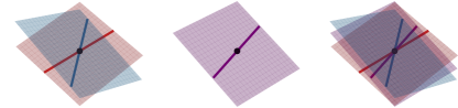
Figure 1: Chordal averaging on the flag manifold $\mathcal{FL}(1,2;3)$. The average (shown in purple) of the input (red and blue) lines remain in the average of the input planes.

A flag manifold is a nested series of subspaces geometrically generalizing Grassmanians. Any multilevel, multiresolution, or multiscale phenomena is likely to involve flags, whether implicitly or explicitly. This makes flag manifolds instrumental in dimensionality reduction, clustering, learning deep feature embeddings, visual domain adaptation, deep neural network compression and dataset analysis [49, 43, 64]. Thus, computing statistics on flag manifolds becomes an essential prerequisite powering several downstream applications. In this paper, we propose an approach for computing first order statistics on (oriented) flag manifolds (c.f. Fig. 1). In particular, endowing flag manifolds with the non-canonical chordal metric, we first transform the (weighted) flag-mean problem into an equivalent minimization on the Stiefel manifold, the space of orthonormal frames, via the method of Lagrange multipliers. We then leverage Riemannian Trust-Region (RTR) optimizers [15, 13] to obtain the solution. Subsequently, we introduce an iteratively reweighted least squares (IRLS) scheme to estimate the more robust flag-median as an $L_{1}$ flag-mean. Finally, we show how several common problems in computer vision such as motion averaging, can be translated onto averages on flag manifolds using group contraction operators [57]. In particular, our contributions are:

• We introduce a new algorithm for computing flag-prototypes (e.g. flag-mean and -median) of a set of points lying on the flag-manifold.

• Analogous to our flag-mean, we introduce an IRLS minimization to estimate the flag-median.

• We prove the convergence of the proposed IRLS algorithm for the flag-median.

• We show how rigid motions can be embedded into flags and thus provide a new way to robustly average motions.

Our diverse experiments reveal that flag averages are more robust, usually yield more reliable estimates, and are more general, i.e., generalize Grassmannian averages. We will release our implementations upon publication.

2 Related Work

Flag manifolds

Besides being mathematically interesting objects [61, 24, 7], flags and flag manifolds have been explored by a series of works from Nishimori et al. addressing subspace independent component analysis (ICA) via Riemannian optimization [53, 55, 52, 56, 52, 54]. Nested sequences of subspaces (e.g. flags) appear in the weights in principal component analysis (PCA) [63] and the result of a wavelet transform [37].

Flag manifolds in computer vision

The utilization of flag manifolds in computer vision is a recent development. Ma et al. [43] employ nested subspace methods to compare large datasets. Additionally, they port self-organizing mappings to work on flag manifolds, enabling parameterization of a set of flags of a fixed type. This method was applied to hyper-spectral image data analysis [44]. Ye et al. [63] derive closed-form analytic expressions for the set of operators required for Riemannian optimization algorithms on the flag manifold, while Nguyen [51] provides algorithms for logarithmic maps and geodesics on flag manifolds. Marrinan et al. [48] investigate the averaging of Grassmanians into flags, demonstrating that flag means behave more like medians and are therefore more robust to the presence of outliers among the subspaces being averaged. Building on this work, they utilize flag averages to improve the detection of chemical plumes in hyperspectral videos [47]. Finally, Mankovich et al. [45] also average Grassmannians into flags by providing the median as a flag and an algorithm to compute it.

3 Chordal Centroids on Flag Manifolds

We begin by providing the necessary definitions related to flag manifolds before presenting our chordal flag-mean and -median algorithms.

Definition 1 (Matrix groups).

The orthogonal group $O(d)$ denotes the group of distance-preserving transformations of a Euclidean space of dimension $d$. $SO(d)$ is the special orthogonal group containing matrices in $O(d)$ determinant $1$. The Stiefel manifold $St(k,d)$, a.k.a. the set of all orthonormal $k$-frames in $\mathbb{R}^{d}$, can be represented as the quotient group: $St(k,d)=O(d)/O(d-k)$. A point on the Stiefel manifold is parameterized by a tall-skinny $d\times k$ real matrix with orthonormal columns. The Grassmannian, $Gr(k,d)$, represents the collection of points parameterizing the $k$-dimensional subspaces of a fixed $d$-dimensional vector space, e.g. $\mathbb{R}^{d}$. For our purposes, $Gr(k,d)$ is a real matrix manifold, where each point is identified with an equivalence class of orthogonal matrices, i.e. $Gr(k,d)=O(d)/O(k)\times O(d-k)$.
Notation: We represent $[\mathbf{X}]\in Gr(k,d)$ using the truncated orthogonal matrix $\mathbf{X}\in\mathbb{R}^{d\times k}$. For this paper $[\mathbf{X}]$ is used to denote the subspace spanned by the columns of $\mathbf{X}$.

Definition 2 (Flag).

A flag in a finite dimensional vector space $\mathcal{V}$ over a field is a sequence of nested subspaces with increasing dimension, each containing its predecessor, i.e. the filtration: $\{\emptyset\}=\mathcal{V}_{0}\subset\mathcal{V}_{1}\subset\dots\subset\mathcal{V}_{k}\subset\mathcal{V}$ with $0=d_{0}<d_{1}<\dots<d_{k}<d_{k+1}=d$ where $\mathrm{dim}\mathcal{V}_{i}=d_{i}$ and $\mathrm{dim}\mathcal{V}=d$. We say this flag is of type or signature $(d_{1},\dots,d_{k},d)$. A flag is called complete if $d_{i}=i,\,\forall i$. Otherwise the flag is incomplete or partial.

Notation: A flag, $[\![\mathbf{X}]\!]$ of type $(d_{1},\dots,d_{k},d)$, is represented by a truncated orthogonal matrix $\mathbf{X}\in\mathbb{R}^{d\times d_{k}}$. Let $m_{j}=d_{j}-d_{j-1}$ for $j=1,2,\dots,k+1$, and $\mathbf{X}_{j}\in\mathbb{R}^{d\times m_{j}}$ for $j=1,2,\dots,k$ whose columns are the $d_{j-1}+1$ to $d_{j}$ columns of $\mathbf{X}$. $[\![\mathbf{X}]\!]$ is

$$[\mathbf{X}_{1}]\subset[\mathbf{X}_{1},\mathbf{X}_{2}]\subset\cdots\subset[\mathbf{X}_{1},\dots,\mathbf{X}_{k}]=[\mathbf{X}]\subset\mathbb{R}^{d}.$$

Definition 3 (Flag manifold).

The aggregate of all flags of the same type, i.e. a certain collection of ordered sets of vector subspaces, admit the structure of manifolds. We refer to this flag manifold as $\mathcal{FL}(d_{1},...,d_{k};d)$ or equivalently as $\mathcal{FL}(d+1)$. The points of $\mathcal{FL}(d+1)$ parameterize all flags of type $(d_{1},...,d_{k},d)$. Flag manifolds generalize Grassmannians because $\mathcal{FL}(k;d)=\mathrm{Gr}(k,d)$. $\mathcal{FL}(d+1)$ can be thought of as a quotient of groups  [44]:

$$\mathcal{FL}(d+1)=SO(d)/S(O(m_{1})\times O(m_{2})\times\cdots\times O(m_{k+1})).$$

Definition 4 (Chordal distance on the flag manifold [58]).

For $[\![\mathbf{X}]\!],[\![\mathbf{Y}]\!]\in\mathcal{FL}(d+1)$, the chordal distance is a map $d_{c}:\mathcal{FL}(d+1)\times\mathcal{FL}(d+1)\to\mathbb{R}$:

$$d_{c}([\![\mathbf{X}]\!],[\![\mathbf{Y}]\!]):=\sqrt{\sum_{j=1}^{k}m_{j}-{\mathrm{tr}}(\mathbf{X}_{j}^{\top}\mathbf{Y}_{j}\mathbf{Y}_{j}^{\top}\mathbf{X}_{j})}.$$ (1)

We now endow flags with orientation, which is required in certain applications such as motion averaging.

Definition 5 (Oriented flag manifold [59, 44]).

An oriented flag manifold, $\mathcal{FL}^{+}(d+1)$, contains only flags with subspaces with compatible orientations. Algebraically:

$$\mathcal{FL}^{+}(d+1)=SO(d)/(SO(m_{1})\times\cdots\times SO(m_{k+1})).$$

Two oriented vector spaces have the same orientation if the determinant of the unique linear transformation between them is positive [6].

3.1 The Chordal Flag-mean

Armed with notation for flags (Dfn. 2) and ways to measure distance between them (Dfn. 4), we are prepared to state the chordal flag-mean estimation problem formally.

Definition 6 (Weighted chordal flag-mean).

Let $\{[\![\mathbf{X}^{(i)}]\!]\}_{i=1}^{p}\subseteq\mathcal{FL}(d+1)$ be a set of points on a flag manifold with weights $\{\alpha_{i}\}_{i=1}^{p}\subset\mathbb{R}$ where $\alpha_{i}\geq 0$. The chordal flag-mean $[\![\bm{\mu}]\!]$ of these points solves:

$$\operatorname*{arg\min}_{[\![\mathbf{Y}]\!]\in\mathcal{FL}(d+1)}\sum_{i=1}^{p}\alpha_{i}d_{c}([\![\mathbf{X}^{(i)}]\!],[\![\mathbf{Y}]\!])^{2}.$$ (2)

Note: for $\mathcal{FL}(k;n)$, this amounts to the Grassmannian-mean by Draper et al. [25].

Proposition 1.

The chordal flag-mean optimization problem in Eq. 2 can be phrased as the Stiefel manifold optimization problem:

$$\operatorname*{arg\min}_{\mathbf{Y}\in St(d_{k},d)}\sum_{j=1}^{k}m_{j}-{\mathrm{tr}}\left(\mathbf{I}_{j}\mathbf{Y}^{\top}\mathbf{P}_{j}\mathbf{Y}\right).$$ (3)

where the matrices $\mathbf{I}_{j}$ and $\mathbf{P_{j}}$ are given below

$$(\mathbf{I}_{j})_{i,l}=\begin{cases}1,&i=l\in\{d_{j-1}+1,d_{j-1}+2,\dots,d_{j}\}\\ 0,&\text{ otherwise}\\ \end{cases},$$

$$\mathbf{P}_{j}=\sum_{i=1}^{p}\alpha_{j}\mathbf{X}_{j}^{(i)}{\mathbf{X}_{j}^{(i)}}^{\top}.$$ (4)

Proof sketch.

We use truncated orthogonal representations for points on the Stiefel and flag manifolds. By the equivalence of minimization problems we write Eq. 2 as

$$\operatorname*{arg\min}_{\mathbf{Y}\in St(d_{k},d)}\sum_{j=1}^{k}m_{j}-\sum_{j=1}^{k}\sum_{i=1}^{p}\alpha_{i}{\mathrm{tr}}\left(\mathbf{Y}_{j}^{\top}\mathbf{X}_{j}^{(i)}{\mathbf{X}_{j}^{(i)}}^{\top}\mathbf{Y}_{j}\right).$$

$\mathbf{I}_{j}$ allows us to write $\mathbf{Y}_{j}\mathbf{Y}_{j}^{\top}=\mathbf{Y}\mathbf{I}_{j}\mathbf{Y}^{\top}$. Using this, properties of trace, and our definition of $\mathbf{P}_{j}$ we write Eq. 2 as Eq. 3.

∎

We provide the full proof in the appendix. We now extend the chordal mean to the case of a certain family of complete and oriented flags.

Proposition 2.

Let $\{\mathbf{x}^{(i)}\}_{i=1}^{p}\subset\mathbb{R}^{d}$. Then suppose ${\mathbf{x}^{(i)}}^{\top}\mathbf{x}^{(j)}>0$ for all $i,j$. Then the naive Euclidean mean $\bm{z}=\frac{1}{n}\sum_{i=1}^{p}\mathbf{x}^{(i)}$ has the same orientation as each $\mathbf{x}^{(i)}$.

Proof.

The proof follows from the simple derivation:

$${\mathbf{x}^{(j)}}^{\top}\bm{z}={\mathbf{x}^{(j)}}^{\top}\frac{1}{n}\sum_{i=1}^{p}\mathbf{x}^{(i)}=\frac{1}{n}\sum_{i=1}^{p}{\mathbf{x}^{(j)}}^{\top}\mathbf{x}^{(i)}>0.$$

∎

Definition 7 ($\mathcal{FL}^{+}(1,\dots,d-1;d)$ chordal flag-mean).

Let $\{[\![\mathbf{X}^{(i)}]\!]\}_{i=1}^{p}\subset\mathcal{FL}(1,2,\dots,d-1;d)$ where for each $j$ and any $i$ and $k$, ${\mathbf{X}_{j}^{(i)}}^{\top}{\mathbf{X}_{j}^{(k)}}>0$. Let $[\![\bm{\mu}]\!]$ be the chordal flag-mean (e.g., Eq. 2) and $\bm{z}_{j}$ be the Euclidean mean of $\{\mathbf{X}_{j}^{(i)}\}_{i=1}^{p}\in\mathbb{R}^{d}$. Then the oriented chordal flag-mean is defined as $[\![\bm{\mu}^{+}]\!]\in\mathcal{FL}^{+}(1,\dots,d-1;d)^{+}$:

$$\bm{\mu}^{+}_{j}=\begin{cases}\mathbf{Y}_{j},&\bm{z}_{j}^{\top}\mathbf{Y}_{j}\geq 0\\ -\mathbf{Y}_{j},&\text{otherwise}.\end{cases}$$ (5)

Remark 1.

The ordering of the columns of $\bm{\mu}$ is the same as that of each $\mathbf{X}^{(i)}$ because the chordal distance on the flag manifold respects the ordering of the vectors in the flag representation by only comparing $\bm{\mu}_{j}$ to $\mathbf{X}_{j}^{(i)}$. So, we only need to correct for the sign of the columns of $\bm{\mu}$. By Prop. 2, we know that the Euclidean mean, $\bm{z}$, has the same orientation as each of $\mathbf{X}_{j}^{(i)}$. We use Eq. 5 to force $\bm{\bm{z}}_{j}^{\top}\bm{\mu}_{j}^{*}\geq 0$. Dfn. 7 gives us a way to choose which chordal flag-mean representatives are best for averaging representations of motions in $\mathcal{FL}^{+}(1,2,3;4)$ in Sec. 4.

Input: Set of points on a flag manifold $\{[\![\mathbf{X}^{(i)}]\!]\}_{i=1}^{p}$

Output: Chordal flag-mean $[\![\bm{\mu}]\!]$

[0.25em] Initialize $[\![\bm{\mu}]\!]$

Compute projections ${\{\mathbf{P}_{i}\}_{i=1}^{k}}$ as in Eq. 4

Define ${\{\mathbf{I}_{i}\}_{i=1}^{k}}$ as in Prop. 1

Optimize Eq. 3 using Stiefel RTR to find $[\![\bm{\mu}]\!]$

Algorithm 1 Chordal flag-mean.

To compute the proposed mean, we optimize Eq. 3 via RTR methods [2, 15] and re-orient the mean using Dfn. 7.

Remark 2.

The geodesic distance averages on the Grassmannian (e.g. $\ell_{2}$-median and Karcher mean) are known to be unique only for certain subsets of the Grassmannian [3]. The proof of this revolves around finding the region of convexity of the geodesic distance function and its square. Uniqueness for Grassmannian chordal distance averages (e.g. the GR-mean [25] and -median [45]) is largely unstudied. It is known that the chordal distance on the Grassmannian approximates the geodesic distance, but its region of convexity is an open problem to the best of our knowledge. Determining the convexity of our chordal flag-mean and -median would boil down to finding the region of convexity of the chordal distance function and its square on the flag manifold. Additionally, one could generalize geodesic distance averages to the flag manifold using Riemannian operators on flags [63], find an algorithm to compute them and their region of convexity. We leave these projects to future work.

3.2 The Chordal Flag-median

We are now ready to provide our iterative algorithm for robust centroid estimation.

Definition 8 (Weighted chordal flag-median).

Let $\{[\![\mathbf{X}^{(i)}]\!]\}_{i=1}^{p}\subseteq\mathcal{FL}(d+1)$ be a set of points on a flag manifold with weights $\{\alpha_{i}\}_{i=1}^{p}\subset\mathbb{R}$ where $\alpha_{i}\geq 0$. The chordal flag-median, $[\![\bm{\eta}]\!]$, of these points solves

$$\operatorname*{arg\min}_{[\![\mathbf{Y}]\!]\in\mathcal{FL}(d+1)}\sum_{i=1}^{p}\alpha_{i}d_{c}([\![\mathbf{X}^{(i)}]\!],[\![\mathbf{Y}]\!]).$$ (6)

Note: for $\mathcal{FL}(k;n)$, this amounts to the Grassmannian-median by Mankovich et al. [45].

Proposition 3.

The flag-median optimization problem in Eq. 6 can be phrased with weights $w_{i}([\![\mathbf{Y}]\!])$ in:

$$w_{i}([\![\mathbf{Y}]\!])=\frac{\alpha_{i}}{\max\{d_{c}([\![\mathbf{X}^{(i)}]\!],[\![\mathbf{Y}]\!]),\epsilon\}},$$ (7)

$$\operatorname*{arg\min}_{[\![\mathbf{Y}]\!]\in\mathcal{FL}(d+1)}\sum_{i=1}^{p}\sum_{j=1}^{k}m_{j}-w_{i}([\![\mathbf{Y}]\!]){\mathrm{tr}}\left(\mathbf{Y}_{j}^{\top}\mathbf{X}_{j}^{(i)}{\mathbf{X}_{j}^{(i)}}^{\top}\mathbf{Y}_{j}\right).$$ (8)

where $\epsilon=0$ as long as $d_{c}([\![\mathbf{X}^{(i)}]\!],[\![\mathbf{Y}]\!])\neq 0$ for all $i$.

Proof sketch.

We can encode the constraints and our optimization problem into the Lagrangian:

$$\begin{aligned} \nabla_{\mathbf{Y}_{j}}\mathcal{L}&=-2\sum_{i=1}^{p}\frac{\alpha_{i}\mathbf{X}_{j}^{(i)}{\mathbf{X}_{j}^{(i)}}^{\top}\mathbf{Y}_{j}}{\sqrt{\sum_{j=1}^{k}m_{j}-{\mathrm{tr}}\left({\mathbf{X}_{j}^{(i)}}^{\top}\mathbf{Y}_{j}\mathbf{Y}_{j}^{\top}\mathbf{X}_{j}^{(i)}\right)}}\\ &+2\sum_{j=1}^{k}\lambda_{i,j}\mathbf{Y}_{i}\mathbf{Y}_{i}^{\top}\mathbf{Y}_{j},\\ \nabla_{\lambda_{i,j}}\mathcal{L}&=m_{j}\delta_{i,j}-{\mathrm{tr}}\left(\mathbf{Y}_{i}^{\top}\mathbf{Y}_{j}\mathbf{Y}_{j}^{\top}\mathbf{Y}_{i}\right).\end{aligned}$$

Then we take the gradient of the Lagrangian with respect to $\mathbf{Y}_{j}$ and $\lambda_{i,j}$ and set it equal to zero. So, for each $j$, we have

$$4m_{j}\lambda_{j,j}=\sum_{i=1}^{p}\frac{\alpha_{i}{\mathrm{tr}}\left(\mathbf{Y}_{j}^{\top}\mathbf{X}_{j}^{(i)}{\mathbf{X}_{j}^{(i)}}^{\top}\mathbf{Y}_{j}\right)}{d_{c}([\![\mathbf{X}^{(i)}]\!],[\![\mathbf{Y}]\!])}.$$

Maximizing each $4m_{j}\lambda_{j,j}$ will minimize the objective function in Eq. 6. We use equivalences of optimization problems to reformulate this maximization as Eq. 8. ∎

Proposition 4.

Fixing $[\![\mathbf{Z}]\!]\in\mathcal{FL}(d+1)$, Eq. 8, with $w_{i}([\![\mathbf{Z}]\!])$, becomes

$$\operatorname*{arg\min}_{[\![\mathbf{Y}]\!]\in\mathcal{FL}(d+1)}\sum_{i=1}^{p}\sum_{j=1}^{k}m_{j}-w_{i}([\![\mathbf{Z}]\!]){\mathrm{tr}}\left(\mathbf{Y}_{j}^{\top}\mathbf{X}_{j}^{(i)}{\mathbf{X}_{j}^{(i)}}^{\top}\mathbf{Y}_{j}\right)$$

and is equivalent to a chordal flag-mean with weights $w_{i}([\![\mathbf{Z}]\!])$. Note: $\epsilon=0$ as long as $d_{c}([\![\mathbf{X}^{(i)}]\!],[\![\mathbf{Z}]\!])\neq 0$ for all $i$.

Proof sketch.

This follows from the proof of Prop. 1. ∎

Input: Set of points on a flag manifold $\{[\![\mathbf{X}^{(i)}]\!]\}_{i=1}^{p}$

Output: Chordal flag-median $[\![\bm{\eta}]\!]$

[0.25em] Initialize $[\![\bm{\eta}]\!]$

while (not converged) do

       Assign $w_{i}([\![\bm{\eta}]\!])$ using Eq. 7 (with $\epsilon>0$)

       $[\![\bm{\eta}]\!]\leftarrow$ flag-mean($\{[\![\mathbf{X}^{(i)}]\!]\},\{w_{i}([\![\bm{\eta}]\!])\}$)

Algorithm 2 Chordal flag-median.

Prop. 3 simplifies our optimization problem to Eq. 8. Given an estimate for the chordal flag-median, $[\![\mathbf{Z}]\!]$, Prop. 4 shows that solving a weighted chordal flag mean problem will approximate the solution to Eq. 8. Using the propositions, we are now ready to present our iterative algorithm for flag-median estimation in Alg. 2.

The convergence of Weiszfeld-type algorithms are well studied in the literature [4, 9, 65] and our IRLS algorithm for the chordal flag-median can be proven to decrease its respective objective function value over iterations. This is what we establish next in Prop. 5, inspired by the proof methods given in [9].

Proposition 5.

Let $[\![\mathbf{Y}]\!]\in\mathcal{FL}(d+1)$. Suppose $d([\![\mathbf{Y}]\!],[\![\mathbf{X}^{(i)}]\!])>\epsilon$ for $i=1,2,\dots,p$. Also define the maps: $T:\mathcal{FL}(d+1)\rightarrow\mathcal{FL}(d+1)$ as an iteration of Alg. 2 and $f:\mathcal{FL}(d+1)\rightarrow\mathbb{R}$ as the chordal flag-median objective function value. Then

$$f(T([\![\mathbf{Y}]\!]))\leq f([\![\mathbf{Y}]\!]).$$ (9)

Proof sketch.

We define the function

$$h([\![\mathbf{Z}]\!],[\![\mathbf{Y}]\!])=\sum_{i=1}^{p}w_{i}([\![\mathbf{Z}]\!])d_{c}([\![\mathbf{X}^{(i)}]\!],[\![\mathbf{Y}]\!])^{2}.$$ (10)

By definition of $h$, $T$, and $f$, we have

$$h(T([\![\mathbf{Y}]\!]),[\![\mathbf{Y}]\!])\leq h([\![\mathbf{Y}]\!],[\![\mathbf{Y}]\!])\leq f([\![\mathbf{Y}]\!]).$$

We use $h$ and $2a-b<\frac{a^{2}}{b}$ for $a,b\in\mathbb{R}$, $b>0$ to find

$$2f(T([\![\mathbf{Y}]\!])-f([\![\mathbf{Y}]\!])\leq h(T([\![\mathbf{Y}]\!]),[\![\mathbf{Y}]\!]).$$

From our string of inequalities, we have the desired result. We leave the full proof to our supplementary material. ∎

Remark 3.

The distance vanishes when $[\![\mathbf{Y}]\!]=[\![\mathbf{X}^{(i)}]\!]$ (e.g., $d_{c}([\![\mathbf{Y}]\!],[\![\mathbf{X}^{(i)}]\!])=0$). In this case, Alg. 2 gets stuck at $[\![\mathbf{X}^{(i)}]\!]$ and the result in Prop. 5 becomes

$$f(T([\![\mathbf{Y}]\!]))\leq f([\![\mathbf{Y}]\!])+{p\epsilon}/{2}.$$ (11)

This singularity can be removed even for a general Weiszfeld iteration, simply by replacing the weights [5].

Proposition 6.

Let $[\![\mathbf{Y}_{k}]\!]\in\mathcal{FL}(d+1)$ be an iterate of Alg. 2 and $f:\mathcal{FL}(d+1)\rightarrow\mathbb{R}$ denote the chordal flag-median objective value. $f([\![\mathbf{Y}_{k}]\!])$ converges as $k\rightarrow\infty$ as long as $d_{c}([\![\mathbf{Y}]\!],[\![\mathbf{X}_{i}]\!])>\epsilon$ for $i=1,2,\dots,p$ and each $k$.

Proof.

Notice that the real sequence with terms $f([\![\mathbf{Y}_{k}]\!])\in\mathbb{R}$ is bounded below by $0$ and is decreasing by Prop. 5. So it converges as $k\rightarrow\infty$. ∎

4 Motion Averaging

In this section, we propose a method for motion averaging by leveraging novel definitions of averages on the flag manifold. This will also act as a good example of how to use flag manifolds for performing computations on other groups. To this end, we now define the group of $3$D rotations and translations, $SE(3)$. Then we outline how to navigate between points on $SE(3)$ and points on a flag. Finally, we describe our motion averaging on flag manifolds.

Definition 9 (3D motion).

The configuration (position and orientation) of a rigid body moving in free space can be described by a homogeneous transformation matrix $\mathbf{M}$ corresponding to the displacement from any inertial reference frame to another. The set of all such rigid body transformations in three-dimensions form the $SE(3)$ group:

$$SE(3)=\left\{\bm{\gamma}:=\begin{bmatrix}\mathbf{R}&\mathbf{t}\\ \mathbf{0}^{\top}&1\end{bmatrix}\,:\,\mathbf{R}\in SO(3)\,\mathrm{\,and\,}\,\mathbf{t}\in\mathbb{R}^{3}\right\},$$

where $\mathbf{t}$ denotes a translation (positional displacement) and $\mathbf{R}$ captures the angular displacements as an element of the special orthogonal group $SO(3)$:

$$SO(3)=\left\{\mathbf{R}\in\mathbb{R}^{3\times 3}\colon\mathbf{R}^{\top}\mathbf{R}=\mathbf{I}\,\wedge\,\det\mathbf{R}=1\right\}.$$ (12)

Proposition 7 (Motion contraction [57]).

We call
$\Phi_{\lambda}:SE(3)\to SO(4)$ a Saletan contraction, i.e. $\Phi_{\lambda}(\bm{\gamma})=\mathbf{U}\mathbf{V}^{T}$ where the left ($\mathbf{U}$) & right ($\mathbf{V}$) singular vectors are obtained via the singular value decomposition:

$$\mathbf{U}\bm{\Sigma}\mathbf{V}^{T}=\begin{bmatrix}\mathbf{R}&\mathbf{t}/\lambda\\ \mathbf{0}^{\top}&1\end{bmatrix}\text{ \emph{for} }\bm{\gamma}\in SE(3).$$ (13)

Proposition 8 (Inverse motion contraction [57]).

We call the inverse contraction map $\Phi_{\lambda}^{-1}:SO(4)\to SE(3)$. Let $\mathbf{M}\in SO(4)$, then $\bm{\gamma}=\Phi_{\lambda}^{-1}(\mathbf{M})$ where

$$\mathbf{t} =\frac{2\lambda}{\mathbf{M}_{4,4}}\mathbf{M}_{1:3,4},$$ (14)

$$\mathbf{R} =\begin{cases}\mathbf{M}_{1:k,1:k},&\|\mathbf{t}\|_{2}<\epsilon\\ \left(\mathbf{M}_{4,4}\frac{\mathbf{t}\mathbf{t}^{T}}{\|\mathbf{t}\|_{2}^{2}}+\mathbf{P^{\prime}}\right)^{-1}\mathbf{M}_{1:k,1:k},&\mathrm{o.w.}\end{cases},$$ (15)

and $\mathbf{U}\bf{\Sigma}\mathbf{V}^{T}=\mathbf{t}^{T}$ is the SVD and $\mathbf{P^{\prime}}=\mathbf{V}_{:,2:4}\mathbf{V}_{:,2:4}^{T}$.

Input: Motions $\{\bm{\gamma}\}_{i=1}^{p}\subset SE(3)$, scale $\lambda\in R$

Output: Average motion $\bm{\gamma^{*}}\in SE(3)$

[0.25em] Compute $\{\Phi_{\lambda}(\gamma_{i})\}_{i=1}^{p}\subset SO(4)$ using Prop. 7

Compute $\left\{[\![\mathbf{X}^{(i)}]\!]\right\}_{i=1}^{p}\subset FL^{+}(1,2,3;4)\}$ from $\{\Phi(\gamma_{i})\}_{i=1}^{p}$ using Prop. 9

Mean:$\quad[\![\mathbf{Y}^{*}]\!]\leftarrow\text{flag-mean}\left(\left\{[\![\mathbf{X}^{(i)}]\!]\right\}_{i=1}^{p}\right)$

Median: $[\![\mathbf{Y}^{*}]\!]\leftarrow\text{flag-median}\left(\left\{[\![\mathbf{X}^{(i)}]\!]\right\}_{i=1}^{p}\right)$

Use Prop. 10 to compute $\mathbf{M}^{\star}\in SO(4)$

Use Prop. 8 to compute $\mathbf{R}^{\star}\in SO(3)$ and $\mathbf{t}^{\star}\in\mathbb{R}^{3}$

Algorithm 3 Motion averaging on Flag manifolds.

Proposition 9 (Flag representation of motion [59]).

Any contracted motion $\mathbf{M}\in SO(4)$ can be represented as a point on the flag, $[\![\mathbf{X}]\!]\in\mathcal{FL}^{+}(1,2,3;4)$ as the first $3$ columns of $\mathbf{M}$. Namely, $[\![\mathbf{X}]\!]$ is

$$\left[\mathbf{m_{1}}\right]\subset\left[\mathbf{m_{1}},\mathbf{m_{2}}\right]\subset\left[\mathbf{m_{1}},\mathbf{m_{2}},\mathbf{m_{3}}\right]\subset\mathbb{R}^{4}.$$ (16)

Remark 4.

Note that the elements of the group of rigid body motions, $SE(3)$, which we represent by points on $SO(4)$, can be imagined as the points of a six-dimensional quadric in seven-dimensional projective space, $\mathbb{P}^{7}$, called the Study quadric [59]. The well known dual quaternions are the very coordinates of this space. Such a bijection between $\mathbb{P}^{7}$ and $SO(4)$ [50] is the reason why our free parameter $\lambda$ resembles the dual unit $\varepsilon$ in dual quaternions [59, 1, 18]. Moreover, our flag manifold, $\mathcal{FL}^{+}(1,2,3;4)$ is homeomorphic to $SO(4)$. We leave the investigation of these deeper connections to future work.

Proposition 10 (Motion representation of a flag [59]).

Given $[\![\mathbf{X}]\!]\in\mathcal{FL}^{+}(1,2,3;4)$ with the same basis vectors from Prop. 9, the corresponding point on $SO(4)$ is

$$\left[\mathbf{m}_{1},\mathbf{m}_{2},\mathbf{m}_{3},\mathbf{z}\right]\in SO(4),$$ (17)

where $\mathbf{z}$ is found by running the Gram-Schmidt process to find a $4^{\text{th}}$ unit vector orthogonal to $\text{span}\{\mathbf{m}_{1},\mathbf{m}_{2},\mathbf{m}_{3}\}$.

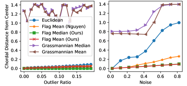
Figure 2: $100$ points from a synthetic data set on $\mathcal{FL}(1,3;10)$. The vertical axis is the chordal distance on $\mathcal{FL}(1,3;10)$ between the predicted averages and the “center” of the data set.

4.1 Single Motion Averaging

With these constructs, we are now ready to formally define the motion averaging problem for points on $SE(3)$.

Definition 10.

Given a set of motions $\{\bm{\gamma}_{i}\in SE(3)\}_{i=1}^{p}$, the centroid is defined to be the solution of the following optimization procedure:

$$\bm{\gamma}^{*}=\operatorname*{arg\min}_{\bm{\gamma}\in SE(3)}\sum_{i=1}^{p}\alpha_{i}\|\bm{\gamma}_{i}-\bm{\gamma}\|^{q}_{\mathrm{F}}$$ (18)

where $q=2$ for mean estimation, $q=1$ for the median and $\alpha_{i}\in\mathbb{R}$ denote the individual weights.

To solve Eq. 18, we simply map each $\bm{\gamma}_{i}\in SE(3)$ to $\mathbf{X}^{(i)}\in FL(1,2,3;4)^{+}$. To this end, we first map each $\bm{\gamma}_{i}$ to $\phi_{\lambda}(\bm{\gamma}_{i})=\mathbf{M}_{i}\in SO(4)$ via Prop. 7 and subsequently use Prop. 9 to represent $\mathbf{M}_{i}$ as $[\![\mathbf{X}^{(i)}]\!]\in FL(1,2,3;4)^{+}$. Then we use our flag-mean ($q=2$) or -median algorithm ($q=1$) to solve

$$[\![\mathbf{Y}^{*}]\!]=\operatorname*{arg\min}_{[\![\mathbf{Y}]\!]\in FL(1,2,3;4)^{+}}\sum_{i=1}^{p}\alpha_{i}d_{c}([\![\mathbf{X}^{(i)}]\!],[\![\mathbf{Y}]\!])^{q}$$ (19)

The desired solution $\bm{\gamma}^{*}\in SE(3)$ is then obtained by first mapping $[\![\mathbf{Y}^{*}]\!]$ back to $\mathbf{M}^{*}\in SO(4)$ via Prop. 10 and subsequently using $\bm{\gamma}^{*}=\phi_{\lambda}^{-1}(\mathbf{M}^{*})$ by Prop. 8. We present this chordal Flag motion averaging in Alg. 3.

5 Results

5.1 Averaging on Flag Manifolds

We first consider examples of data naturally existing as flags. We work with $5$ data sets: $2$ synthetic ones, MNIST digits [23], the Yale Face Database [10], and the Cats and Dogs dataset [62]. We provide further evaluation of our flag averages that result in improved clustering on the UFC YouTube dataset [42] in the supplementary material. In one synthetic experiment, we compare our Stiefel Riemannian Trust-Regions (RTR) method in Alg. 1 for computing the flag-mean to the Flag RTR by Nguyen et al. [51]. In the rest of the experiments, we compare our chordal flag (FL)-mean & -median to the Grassmannian (GR)-mean [25] & -median [45], as well as Euclidean averaging, where the matrices are simply averaged and projected onto the flag manifold via QR decomposition. GR-means and -medians, [25, 45] input data a points on Grassmannians by using the largest dimensional subspace in the flag ($[\mathbf{X}^{(i)}]\in\mathrm{Gr}(k,d)$) and output an average as a flag of type $(1,2,\dots,k,d)$. So all the methods considered in this section result in averages which live on a flag manifold. In this section we compare methods for data representation: the flag vs. Grassmannian vs. Euclidean space.

	Dist. to $\mathbf{C}$	Obj. Fn. Value
Ours	$(1.4\pm 0.2)\times 10^{-4}$	$(2.1\pm 0.05)\times 10^{-4}$
[51]	$(3.0\pm 2.1)\times 10^{-3}$	$(1.6\pm 1.6)\times 10^{-3}$

Table 1: Robustness to initialization: Alg. 1 versus Flag RTR from Nguyen et al. [51]. Data: $100$ points on $\mathcal{FL}(1,2,3;10)$.

Synthetic data

Both our synthetic experiments use the same methodology for generating data sets on the Grassmannian and flag. We begin by computing a “center” representative, $\mathbf{C}\in\mathbb{R}^{10\times 3}$, as the first $3$ columns of the QR decomposition of a random matrix in $\mathbb{R}^{10\times 3}$ with entries sampled from the uniform distribution over $[-.5,.5)$, $\mathcal{U}[-.5,.5)$. The representative for the $i^{\text{th}}$ data point, $\mathbf{X}_{i}$, is computed by sampling $\mathbf{Z}_{i}\in\mathbb{R}^{10\times 3}$ with entries from $\mathcal{U}[-.5,.5)$ and defined as the first $3$ columns of the QR decomposition of $\mathbf{C}+\delta\mathbf{Z}_{i}$ for a noise parameter $\delta\geq 0$.

Averaging synthetic flag data

We use synthetic data sets with $100$ points, on $\mathrm{Gr}(3;10)$ and $\mathcal{FL}(1,3;10)$. For the left plot in Fig. 2 we vary $\delta$ to compute our data sets. For the right plot we have $m$ outliers computed with $\delta=1$ and the rest of the data are computed with $\delta=0.001$. We compute the error as the chordal distance on $\mathcal{FL}(1,3;10)$ between the predicted average and $[\![\mathbf{C}]\!]$. In addition to comparing our averages to Grassmannian (GR) averages, we compare Alg. 1 to Nguyen et al. [51] for computing the flag-mean. Our results indicate that our algorithm improves both upon GR, Euclidean, and Nguyen et al. [51] averages in the sense that flag averages are closer to $[\![\mathbf{C}]\!]$. Specifically, our flag-median is more robust to outliers than our flag-mean. Note: Euclidean out preforms GR averaging because Euclidean averaging respects column order (e.g., the flag structure) for matrix representatives of the data, whereas GR averaging does not.

Comparisons to Riemannian flag optimization

In a second experiment, we compare the convergence of Alg. 1 to that of Flag RTR [51]. To this end, we generate $100$ points on $\mathcal{FL}(1,2,3;10)$ using $\delta=0.001$ and run $50$ random trials with different initializations and compute $3$ items (i) the number of iterations to convergence, (ii) the chordal distance on $\mathcal{FL}(1,2,3;10)$ between the flag-mean and $[\![\mathbf{C}]\!]$, (iii) the cost function values from Eq. 2. We find that in every experiment Alg. 1 converges in 2 iterations and Flag RTR converges, on average, in $9.74\pm 2.76$ iterations. In Tab. 1 we see that our method is one order of magnitude closer to the ground truth centroid $[\![\mathbf{C}]\!]$ and produces a one order of magnitude smaller objective function value.

Averaging under varying illumination

To further demonstrate the efficacy of our averages over the standard Grassmanians, we leverage face images from Yale Face Database [10] with central ($c$), left ($l$), and right ($r$) illuminations, respectively. Let $\mathbf{A_{c}},\mathbf{A_{l}},\mathbf{A_{r}}\in\mathbb{R}^{243\times 320}$ be these three images of a person. We represent a face as a point $[\![\mathbf{X}]\!]\in\mathcal{FL}(1,3;d)$ as $[\![\mathbf{X}]\!]=[\mathbf{X}_{1}]\subset[\mathbf{X}]\subset\mathbb{R}^{d}$ and as $[\mathbf{X}]\in\mathrm{Gr}(3,d)$ using the following three steps: (i) Set $\mathbf{v_{i}}=\text{vec}\left(\mathbf{A_{i}}\right)$ for $i=c,l,r$; (ii) take $\mathbf{X}=\mathbf{Q}_{:,1:3}$ where $\mathbf{Q}$ is from the QR decomposition of $[\mathbf{v_{c}},\mathbf{v_{l}},\mathbf{v_{r}}]$. Repeating this process for three faces gives us three points: $[\mathbf{X}_{1}],[\mathbf{X}_{2}],[\mathbf{X}_{3}]\in\mathrm{Gr}(3,d)$ and $[\![\mathbf{X}_{1}]\!],[\![\mathbf{X}_{2}]\!],[\![\mathbf{X}_{3}]\!]\in\mathcal{FL}(1,3;d)$. Then we calculate the Grassmannian-mean of the points in $\mathrm{Gr}(3,d)$ which is the flag: $[\![\bm{\nu}]\!]=[\bm{\nu}_{1}]\subset[\bm{\nu}_{1},\bm{\nu}_{2}]\subset[\bm{\nu}_{1},\bm{\nu}_{2},\bm{\nu}_{3}]$ and the flag-mean (ours) of the points in $\mathcal{FL}(1,3;d)$: $[\![\bm{\mu}]\!]=[\bm{\mu}_{1}]\subset[\bm{\mu}_{1},\bm{\mu}_{2},\bm{\mu}_{3}]$. A plot of reshaped $\bm{\mu}_{1}$ and $\bm{\nu}_{1}$ for a set of three faces in Fig. 3. We would expect the first dimension of both means to look like a face with center illumination. However, only the flag-mean appears to be center-illuminated.

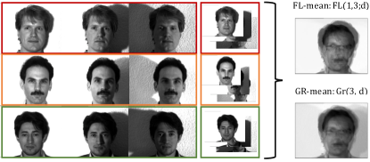
Figure 3: Averaging a collection of faces belonging to three different people, captured under varying illumination: center, left and right. Notice that the first dimension of the flag representations is center illuminated, better representing the mean compared to Grassmannian.

MNIST representation

We run two experiments similar to what was done in [45] with MNIST digits. However, our representations differ since we represent a digit as $[\mathbf{X}_{j}]\in\mathrm{Gr}(2,784)$ and $[\![\mathbf{X}_{j}]\!]\in\mathcal{FL}(1,2;784)$. We generate $p$ representations of a digit, $\{\mathbf{X}_{j}\}_{j=1}^{p}$, by sampling a set of $p$ images without replacement from the test partition. Then we vectorize each image into $\mathbf{v}_{j}\in\mathbb{R}^{784}$ and run $k$ nearest neighbors on $\{\mathbf{v_{j}}\}_{i=1}^{p}$ with $k=2$ using the cosine distance. Say $\mathbf{v}_{j}$ and $\mathbf{v}_{k}$ are the $2$ nearest neighbors of $\mathbf{v}_{j}$, then the representation for sample $j$ is $\mathbf{X}_{j}=\mathbf{Q}_{:,:2}$ from the QR decomposition of $[\mathbf{v}_{j},\mathbf{v}_{k}]$.

Robustness to Neural Network (NN) predictions

For the first MNIST experiment, we use the method above to create $20$ data sets on $\mathrm{Gr}(2,784)$ and $\mathcal{FL}(1,2;784)$ corresponding to $i=0,1,2,\dots,19$. The $i$th data set contains $20$ representations of the digit $1$ and $i$ representations for the digit $9$. We calculate a GR-mean and -median of each of the $i$ data sets on $\mathrm{Gr}(2,784)$ and our flag-mean and -median for the data sets on $\mathcal{FL}(1,2,784)$. Note: all of these averages live on $\mathcal{FL}(1,2,784)$. We then use a NN (trained on the original training data and producing a $97\%$ test accuracy on the original test data) to predict the label of the first dimension of each average for $i=0,1,2,\dots,19$. As plotted in Fig. 4, the NN incorrectly predicts the class of the GR-mean and -median for each data set. In contrast, the flag-mean and -median are all predicted as $1$s with data sets with fewer than $11$ representations of the $9$s digits. The flag-mean is the first flag average to be incorrectly predicted, since it is not as robust to outliers as the flag-median.

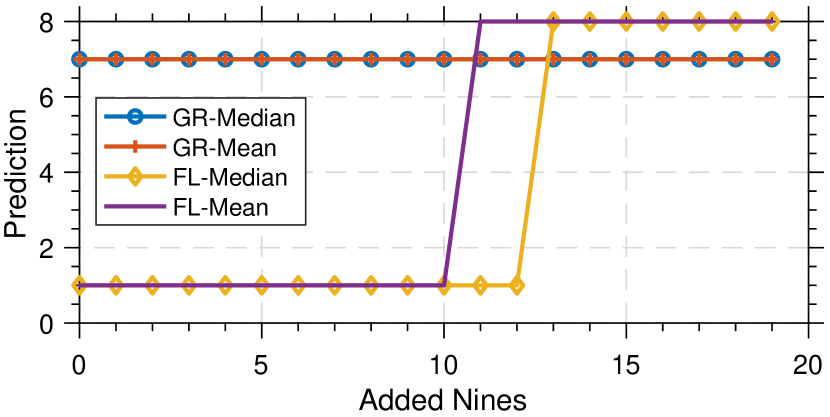
Figure 4: Neural network predictions for the first dimension of different averages $i=0,1,2,\dots,19$ MNIST data sets. The $i$th data set has $i$ representations of the $9$s digit and $20$ representations of the $1$s digit.

Visualizing robustness

Our second MNIST experiment is with $20$ representations of $6$s and with $i$ outlier representations of $7$s for $i=0,4,8,12$. We use the workflow from Fig. 4 to represent the MNIST digits on $\mathrm{Gr}(2,748)$ and $\mathcal{FL}(1,2;748)$. For each $i$, we compute averages of a data set with $i$ representations of $7$s. A chordal distance matrix on $\mathcal{FL}(1,2;798)$ between all the averages and data is used to preform Multidimensional Scaling (MDS) [38] for visualization in Fig. 5. The best averages should barely move (right to left) as we add outlier representations of $7$s. Our flag-mean and -median are moved the least with the addition of representations of $7$s with the median moving less than the mean. In contrast, the Grassmannian-mean and -median [45] move more than the compared baselines as we add $7$s.

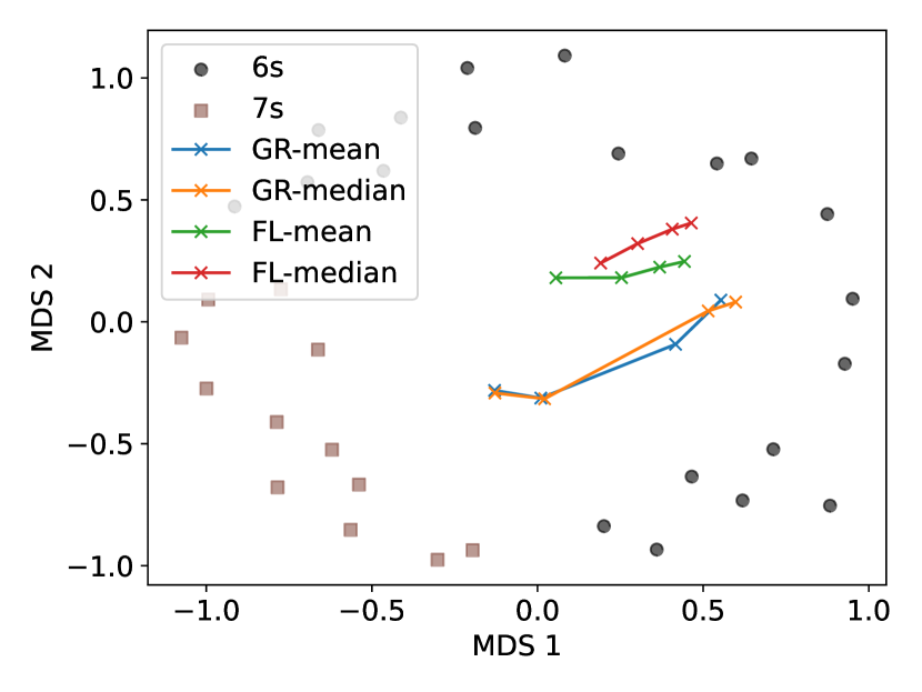
Figure 5: MDS embedding of MNIST digits and Grassmannian and flag averages. Each “x” is an average of $20$ representations of $6$s as we gradually add $i$ outlier representations of $7$s for $i=0,4,8,12$ data sets. The averages move from right to left as we add more $7$s.

PCA by flag statistics

We use the Cats and Dogs dataset [62] to compute $3$-dimensional PCA [35] weights, $\mathbf{W}^{*}\in\mathbb{R}^{4096\times 3}$, of the data matrix, $\mathbf{X}\in\mathbb{R}^{198\times 4096}$. Then we randomly split the $m$ subjects into $p$ evenly sized groups to generate $p$ data matrices each of size $p_{i}$: $\{\mathbf{X_{i}}\}_{i=1}^{p}\subset\mathbb{R}^{p_{i}\times 4096}$. PCA weights of each $\mathbf{X_{i}}$ are computed as $\mathbf{W_{i}}\in\mathbb{R}^{4096\times 3}$. $\mathbf{W}^{*}$ is predicted by averaging $\{\mathbf{W_{i}}\}_{i=1}^{p}$ as points on $\mathcal{FL}(1,2,3;4096)$ and $\mathrm{Gr}(3;4096)$. Specifically, we compute the flag-mean (ours), Grassmannian-mean, Euclidean-mean, and a random point. Then we record the chordal distance on $\mathcal{FL}(1,2,3;4096)$ (reconstruction error) between the average and $[\![\mathbf{W}^{*}]\!]\in\mathcal{FL}(1,2,3;4096)$. Our flag-mean is closer to $[\![\mathbf{W}^{*}]\!]$ for $p=1,2,\dots,6$.

5.2 Averaging Rigid Motions

We now evaluate our algorithm in robust averaging of a set of points represented on the $SE(3)$-manifold. To this end, we synthesize a dataset of 400 rigid motions (rotations and translations) around multiple randomly drawn central points in $SE(3)$. These points are generated with increasing noise levels. Particularly, for rotations we perturb the rotation axis using variances of $[0,5,10,15,20,25]$ degrees, while the translations are perturbed in the levels of $[0,0.02,0.05,0.1,0.2,0.3]$. For each noise level, we run 50 experiments and use $\lambda=1$ to ensure that translations and rotations are well balanced. We then run our algorithms for the flag-mean and -median. These algorithms are compared to standard Govindu [29], and baseline (QT) where translations and quaternions are averaged independently using Markley’s method [46]. We also ran dual quaternion averaging of Torsello et al. [60] and found it produced identical results to Govindu. Our results in Fig. 7 show that both of our algorithms surpass classical motion averages with our flag-median producing more robust estimates.

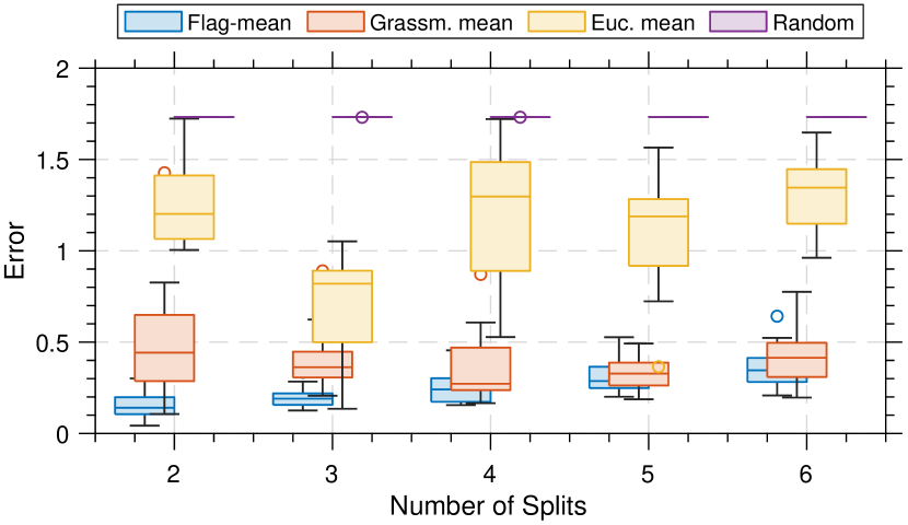
Figure 6: Reconstruction error for PCA weights as a function of Number of Splits, $p$.

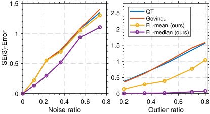
Figure 7: Single motion averaging experiments for increasing levels of $SE(3)$-noise and outlier ratios.

6 Conclusion

We have provided two algorithms, the flag-mean & flag-median, that estimate flag-prototypes of points defined on flag manifolds using chordal distance. We have established the convergence of our IRLS algorithm yielding the flag-median. Our methodologies deviate from the existing literature [25, 45] which average Grassmannians into flags, and are found to be useful when either inherent outlier-robustness is necessary or when the subspaces possess a natural order, (e.g., hierarchical data). Since flag manifolds generalize Grassmannians, our methods can average on a broader class of manifolds. Consequently, we have applied our averages to rigid motions via group contraction.

Limitations & future work

Our method can become computationally expensive when applied to high-dimensional problems. Moreover, our convergence results are weaker than desired as we have not provided a convergence rate. Besides addressing these, our future work involves clustering and inference on data with hierarchical structures.

Acknowledgements

Benjamin Busam introduced Nathan and Tolga during CVPR 2022 in New Orleans. This gracious act is the catalyst in the realization of this work.

Appendices

Appendix A Flag Representations

A flag is a nested collection of subspaces of increasing dimension. An illustration of a $\mathcal{FL}(1,2;3)$ is in Fig. 8).

Flags are a natural representation for time series data as nested “time subspaces.” Suppose we data at three times: $\mathbf{x}_{t=1},\mathbf{x}_{t=2},\mathbf{x}_{t=3}\in\mathbb{R}^{d}$. We can group these data based on their “effect over time” in the sense that time $t=1$ stands alone, $t=1$ affects $t=2$, and $t=1$ and $t=2$ affect $t=3$. This grouping gives us the flag of type $\mathcal{FL}(1,2,3:d)$:

$$\text{span}\{\mathbf{x}_{1}\}\subset\text{span}\{\mathbf{x}_{1},\mathbf{x}_{2}\}\subset\{\mathbf{x}_{1},\mathbf{x}_{2},\mathbf{x}_{3}\}\subset\mathbb{R}^{d}.\vspace{-2.5mm}$$ (20)

Flags can also model some hierarchical data using hierarchically nested subspaces. For a nice list of flags in mathematics, see [63].

Recall $\mathcal{FL}(d+1)=\mathcal{FL}(d_{1},d_{2},\dots,d_{k};d_{k+1}=d)$, we take $m_{1}=1$ and $m_{j}=d_{j}-d_{j-1}$. There are number of representations for flag manifolds involving quotients  [63]. We mention the most popular representation in the manuscript. A number works [43, 44, 63] use

$$\frac{SO(d)}{S(O(m_{1})\times O(m_{2})\times\cdots\times O(m_{k+1}))}$$ (21)

where $S(O(m_{1})\times\dots\times O(m_{k}))$ is

$$\{(\mathbf{M}_{1},\dots,\mathbf{M}_{k})\>:\>\prod_{i=1}^{k}\det(\mathbf{M}_{i})=1\}.\vspace{-1.8mm}$$ (22)

Other works [58, 51] represent flag manifolds using the quotient

$$\frac{St(d_{k},d)}{O(m_{1})\times O(m_{2})\times\cdots\times O(m_{k})}.$$ (23)

In this representation, $\mathbf{X}\in St(d_{k},d)$ is used to represent the equivalence class

$$[\![\mathbf{X}]\!]=\left\{\mathbf{X}\mathbf{O}\>:\>\mathbf{O}_{i}\in O(m_{i})\right\}\in\mathcal{FL}(d+1)$$

where $\mathbf{O}=\text{diag}(\mathbf{O}_{m_{1}},\dots,\mathbf{O}_{m_{k}})$. We use this Stiefel quotient representation in this manuscript.

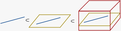
Figure 8: Illustration of a nested sequence of subspaces corresponding to a point on the flag manifold.

Ye et al. prove that $\mathcal{FL}(d+1)$ is diffeomorphic to Eqs. 21 and 23 (see Prop. 4 and 12 in [63]). Additionally, Ye et al. prove that flags are a closed submanifold of

$$\mathrm{Gr}(m_{1},d)\times\mathrm{Gr}(m_{2},d)\times\cdots\mathrm{Gr}(m_{k},d).$$ (24)

Our chordal distance on flag manifolds leverages this product-of-Grassmannians since it is the $2$-norm of the chordal distances between each $\mathrm{Gr}(m_{1},d)$.

Appendix B Proof of Proposition I

Before providing the full proof, let us recall Prop. I:

Proposition 11.

The chordal flag-mean of $\left\{[\![\mathbf{X}_{i}]\!]\right\}_{i=1}^{p}\subset\mathcal{FL}(d+1)$ is

$$\left[\![\bm{\mu}\right]\!]:=\operatorname*{arg\min}_{[\![\mathbf{Y}]\!]\in\mathcal{FL}(d+1)}\sum_{i=1}^{p}\alpha_{i}d_{c}([\![\mathbf{X}^{(i)}]\!],[\![\mathbf{Y}]\!])^{2}$$ (25)

and can be phrased into a Stiefel manifold optimization problem as

$$\left[\bm{\mu}\right]=\operatorname*{arg\min}_{\mathbf{Y}\in St(d_{k},d)}\sum_{j=1}^{k}m_{j}-{\mathrm{tr}}\left(\mathbf{I}_{j}\mathbf{Y}^{\top}\mathbf{P}_{j}\mathbf{Y}\right)$$ (26)

where the matrices $\mathbf{I}_{j}$ and $\mathbf{P_{j}}$ are given in Eq. 27 and Eq. 28 respectively.

$$(\mathbf{I}_{j})_{i,l}=\begin{cases}1,&i=l\in\{d_{j-1}+1,d_{j-1}+2,\dots,d_{j}\}\\ 0,&\text{ otherwise}\\ \end{cases}$$ (27)

and define:

$$\mathbf{P}_{j}=\sum_{i=1}^{p}\alpha_{j}\mathbf{X}_{j}^{(i)}{\mathbf{X}_{j}^{(i)}}^{\top}$$ (28)

For example, if we are averaging on $\mathcal{FL}(1,3;4)$ we have

$$\mathbf{I}_{1}=\begin{bmatrix}1&0&0\\ 0&0&0\\ 0&0&0\end{bmatrix}\mathrm{\quad and\quad}\mathbf{I}_{2}=\begin{bmatrix}0&0&0\\ 0&1&0\\ 0&0&1\end{bmatrix}.$$

Proof.

We begin by realizing Eq. 25 as an optimization problem using the definition of chordal distance:

$$\operatorname*{arg\min}_{[\![\mathbf{Y}]\!]\in\mathcal{FL}(d+1)}\sum_{i=1}^{p}\alpha_{i}\left(\sum_{j=1}^{k}m_{j}-{\mathrm{tr}}\left({\mathbf{X}_{j}^{(i)}}^{\top}\mathbf{Y}_{j}\mathbf{Y}_{j}^{\top}\mathbf{X}_{j}^{(i)}\right)\right).$$

Then we move our summations around to simplify our objective function:

$$\sum_{i=1}^{p}\alpha_{i}\left(\sum_{j=1}^{k}m_{j}-{\mathrm{tr}}\left(\mathbf{Y}_{j}^{\top}\mathbf{X}_{j}^{(i)}{\mathbf{X}_{j}^{(i)}}^{\top}\mathbf{Y}_{j}\right)\right)$$

$$=\sum_{j=1}^{k}\left(\sum_{i=1}^{p}\alpha_{i}\right)m_{j}-\sum_{i=1}^{p}\alpha_{i}{\mathrm{tr}}\left(\mathbf{Y}_{j}^{\top}\mathbf{X}_{j}^{(i)}{\mathbf{X}_{j}^{(i)}}^{\top}\mathbf{Y}_{j}\right),$$

$$=\sum_{j=1}^{k}\left(\sum_{i=1}^{p}\alpha_{i}\right)m_{j}-\sum_{j=1}^{k}\sum_{i=1}^{p}\alpha_{i}{\mathrm{tr}}\left(\mathbf{Y}_{j}^{\top}\mathbf{X}_{j}^{(i)}{\mathbf{X}_{j}^{(i)}}^{\top}\mathbf{Y}_{j}\right).$$

Since $\sum_{i=1}^{p}\alpha_{i}$ is constant with respect to $[\![\mathbf{Y}]\!]$, Eq. 25 is equivalent to

$$\operatorname*{arg\min}_{[\![\mathbf{Y}]\!]\in\mathcal{FL}(d+1)}\sum_{j=1}^{k}m_{j}-\sum_{j=1}^{k}\sum_{i=1}^{p}\alpha_{i}{\mathrm{tr}}\left(\mathbf{Y}_{j}^{\top}\mathbf{X}_{j}^{(i)}{\mathbf{X}_{j}^{(i)}}^{\top}\mathbf{Y}_{j}\right).$$

Using our definitions for $\mathbf{I}_{j}$ and $\mathbf{P}_{j}$, we can write the objective function in terms of $\mathbf{Y}$:

$$\sum_{j=1}^{k}m_{j}-{\mathrm{tr}}\left(\mathbf{Y}_{j}^{\top}\left(\sum_{i=1}^{p}\alpha_{i}\mathbf{X}_{j}^{(i)}{\mathbf{X}_{j}^{(i)}}^{\top}\right)\mathbf{Y}_{j}\right),$$

$$=\sum_{j=1}^{k}m_{j}-{\mathrm{tr}}\left(\mathbf{Y}_{j}^{\top}\mathbf{P}_{j}\mathbf{Y}_{j}\right),$$

$$=\sum_{j=1}^{k}m_{j}-{\mathrm{tr}}\left(\mathbf{Y}_{j}\mathbf{Y}_{j}^{\top}\mathbf{P}_{j}\right),$$

$$=\sum_{j=1}^{k}m_{j}-{\mathrm{tr}}\left(\mathbf{Y}\mathbf{I}_{j}\mathbf{Y}^{\top}\mathbf{P}_{j}\right).$$

The third equality is true because $\mathbf{Y}_{j}\mathbf{Y}_{j}^{\top}=\mathbf{Y}\mathbf{I}_{j}\mathbf{Y}^{\top}$.

There are two constraints for $[\![\mathbf{Y}]\!]\in\mathcal{FL}(d+1)$ according to our representation for points on the flag manifold. The first constraint is $\mathbf{Y}_{j}^{\top}\mathbf{Y}_{j}=\mathbf{I}$ for $j=1,2,\dots,p$. The second constraint is $[\mathbf{Y}_{j}]\cap[\mathbf{Y}_{i}]=\emptyset$ for all $i\neq j$. These constraints are satisfied when $\mathbf{Y}^{\top}\mathbf{Y}=\mathbf{I}$, e.g. $\mathbf{Y}\in St(d_{k},d)$.

Using trace invariance to cyclic permutations, the chordal flag mean optimization problem Eq. 25 is equivalent to the Stiefel optimization problem Eq. 26. ∎

Appendix C Proof of Proposition III

Proposition 12.

The chordal flag-median of $\left\{[\![\mathbf{X}_{i}]\!]\right\}_{i=1}^{p}\subset\mathcal{FL}(d+1)$,

$$\left[\![\bm{\eta}]\right]=\operatorname*{arg\min}_{[\![\mathbf{Y}]\!]\in\mathcal{FL}(d+1)}\sum_{i=1}^{p}\alpha_{i}d_{c}([\![\mathbf{X}^{(i)}]\!],[\![\mathbf{Y}]\!]),$$ (29)

can be phrased with weights

$$w_{i}([\![\mathbf{Y}]\!])=\sum_{j=1}^{k}\frac{\alpha_{i}}{\max\{d_{c}([\![\mathbf{X}^{(i)}]\!],[\![\mathbf{Y}]\!]),\epsilon\}}$$

as the optimization problem

$$\operatorname*{arg\min}_{[\![\mathbf{Y}]\!]\in\mathcal{FL}(d+1)}\sum_{i=1}^{p}\sum_{j=1}^{k}m_{j}-w_{i}([\![\mathbf{Y}]\!]){\mathrm{tr}}\left(\mathbf{Y}_{j}^{\top}\mathbf{X}_{j}^{(i)}{\mathbf{X}_{j}^{(i)}}^{\top}\mathbf{Y}_{j}\right)$$

with $\epsilon=0$ as long as $d_{c}([\![\mathbf{X}^{(i)}]\!],[\![\mathbf{Y}]\!])\neq 0$ for all $i$.

Proof.

We can write Eq. 29 using the definition of chordal distance as

$$\operatorname*{arg\min}_{[\![\mathbf{Y}]\!]\in\mathcal{FL}(d+1)}\sum_{i=1}^{p}\alpha_{i}\sqrt{\sum_{j=1}^{k}m_{j}-{\mathrm{tr}}\left({\mathbf{X}_{j}^{(i)}}^{\top}\mathbf{Y}_{j}\mathbf{Y}_{j}^{\top}\mathbf{X}_{j}^{(i)}\right)}.$$

The orthogonality constraints for $\mathbf{Y}\in\mathbb{R}^{d\times d_{k}}$ to represent a point on $\mathcal{FL}(d+1)$ are: (i) $[\mathbf{Y}_{j}]\cap[\mathbf{Y}_{i}]=\emptyset$ for all $i\neq j$ and $\mathbf{Y}_{j}^{\top}\mathbf{Y}_{j}=\mathbf{I}$ for all $j$. Let $\theta([\mathbf{Y}_{i}],[\mathbf{Y}_{j}])$ denote the vector of principal angles between $[\mathbf{Y}_{i}]$ and $[\mathbf{Y}_{j}]$. Using ${\mathrm{tr}}(\mathbf{Y}_{i}^{\top}\mathbf{Y}_{j}\mathbf{Y}_{j}^{\top}\mathbf{Y}_{i})=\|\cos\theta([\mathbf{Y}_{i}],[\mathbf{Y}_{j}])\|_{2}^{2}$, we encode our orthogonality constraints as

$${\mathrm{tr}}(\mathbf{Y}_{i}^{\top}\mathbf{Y}_{j}\mathbf{Y}_{j}^{\top}\mathbf{Y}_{i})=\begin{cases}0&i\neq j\\ d_{j}&i=j\end{cases}.$$

We will now use

$$\delta_{i,j}=\begin{cases}1,&i=j\\ 0,&i\neq j.\end{cases}$$

to put these constraints into the Lagrangian.

Let $\bm{\Lambda}$ be a symmetric matrix of Lagrange multipliers corresponding to the orthogonality constraints. Denote the entry in the $i$th row and $j$th column of $\bm{\Lambda}$ as $\lambda_{i,j}$. With the constraints added to the objective, we define the Lagrangian in Eq. C.

$$\mathcal{L}(\mathbf{Y},\Lambda) =\sum_{i=1}^{p}\alpha_{i}\sqrt{\sum_{j=1}^{k}m_{j}-{\mathrm{tr}}\left({\mathbf{X}_{j}^{(i)}}^{\top}\mathbf{Y}_{j}\mathbf{Y}_{j}^{\top}\mathbf{X}_{j}^{(i)}\right)}$$

$$-\sum_{i=j}^{k}\sum_{j=1}^{k}\lambda_{i,j}(m_{j}\delta_{i,j}-{\mathrm{tr}}(\mathbf{Y}_{i}^{\top}\mathbf{Y}_{j}\mathbf{Y}_{j}^{\top}\mathbf{Y}_{i})).$$ (30)

The gradient of Eq. C w.r.t. ${\mathbf{Y}_{j}}$ and ${\lambda_{i,j}}$ is

$$\begin{aligned} \nabla_{\mathbf{Y}_{j}}\mathcal{L}&=-\sum_{i=1}^{p}\frac{\alpha_{i}\mathbf{X}_{j}^{(i)}{\mathbf{X}_{j}^{(i)}}^{\top}\mathbf{Y}_{j}}{\sqrt{\sum_{j=1}^{k}m_{j}-{\mathrm{tr}}\left({\mathbf{X}_{j}^{(i)}}^{\top}\mathbf{Y}_{j}\mathbf{Y}_{j}^{\top}\mathbf{X}_{j}^{(i)}\right)}}\\ &+2\sum_{\begin{subarray}{c}i=1\\ i\neq j\end{subarray}}^{k}\lambda_{i,j}\mathbf{Y}_{i}\mathbf{Y}_{i}^{\top}\mathbf{Y}_{j}+4\lambda_{j,j}\mathbf{Y}_{j}\mathbf{Y}_{j}^{\top}\mathbf{Y}_{j},\\ \nabla_{\lambda_{i,j}}\mathcal{L}&=m_{j}\delta_{i,j}-{\mathrm{tr}}\left(\mathbf{Y}_{i}^{\top}\mathbf{Y}_{j}\mathbf{Y}_{j}^{\top}\mathbf{Y}_{i}\right).\end{aligned}$$

Notice we are not dividing by zero because $d_{c}([\![\mathbf{X}^{(i)}]\!],[\![\mathbf{Y}]\!])\neq 0$ for all $i$. Now we use $\nabla_{\mathbf{Y}_{j}}\mathcal{L}=\bm{0}$ and $\nabla_{\lambda_{i,j}}\mathcal{L}=0$ to solve for $\lambda_{j,j}$.

First we will work with $\nabla_{\mathbf{Y}_{j}}\mathcal{L}=\bm{0}$.

$$\begin{aligned} \mathbf{0}&=-\sum_{i=1}^{p}\frac{\alpha_{i}\mathbf{X}_{j}^{(i)}{\mathbf{X}_{j}^{(i)}}^{\top}\mathbf{Y}_{j}}{d_{c}([\![\mathbf{X}^{(i)}]\!],[\![\mathbf{Y}]\!])}\\ &+2\sum_{\begin{subarray}{c}i=1\\ i\neq j\end{subarray}}^{k}\lambda_{i,j}\mathbf{Y}_{i}\mathbf{Y}_{i}^{\top}\mathbf{Y}_{j}+4\lambda_{j,j}\mathbf{Y}_{j}\mathbf{Y}_{j}^{\top}\mathbf{Y}_{j},\\ &=-\sum_{i=1}^{p}\frac{\alpha_{i}\mathbf{Y}_{j}^{\top}\mathbf{X}_{j}^{(i)}{\mathbf{X}_{j}^{(i)}}^{\top}\mathbf{Y}_{j}}{d_{c}([\![\mathbf{X}^{(i)}]\!],[\![\mathbf{Y}]\!])}\\ &+2\sum_{\begin{subarray}{c}i=1\\ i\neq j\end{subarray}}^{k}\lambda_{i,j}\mathbf{Y}_{j}^{\top}\mathbf{Y}_{i}\mathbf{Y}_{i}^{\top}\mathbf{Y}_{j}+4\lambda_{j,j}\mathbf{Y}_{j}^{\top}\mathbf{Y}_{j}\mathbf{Y}_{j}^{\top}\mathbf{Y}_{j},\\ 0&=-\sum_{i=1}^{p}\frac{\alpha_{i}{\mathrm{tr}}\left(\mathbf{Y}_{j}^{\top}\mathbf{X}_{j}^{(i)}{\mathbf{X}_{j}^{(i)}}^{\top}\mathbf{Y}_{j}\right)}{d_{c}([\![\mathbf{X}^{(i)}]\!],[\![\mathbf{Y}]\!])}\\ &+2\sum_{\begin{subarray}{c}i=1\\ i\neq j\end{subarray}}^{k}\lambda_{i,j}{\mathrm{tr}}\left(\mathbf{Y}_{j}^{\top}\mathbf{Y}_{i}\mathbf{Y}_{i}^{\top}\mathbf{Y}_{j}\right)+4\lambda_{j,j}{\mathrm{tr}}\left(\mathbf{Y}_{j}^{\top}\mathbf{Y}_{j}\mathbf{Y}_{j}^{\top}\mathbf{Y}_{j}\right).\\ \end{aligned}$$

Using $\nabla_{\lambda_{i,j}}\mathcal{L}=0$ simplifies our equation to

$$4\lambda_{j,j}{\mathrm{tr}}(\mathbf{Y}_{j}^{\top}\mathbf{Y}_{j}\mathbf{Y}_{j}^{\top}\mathbf{Y}_{j}) =\sum_{i=1}^{p}\frac{\alpha_{i}{\mathrm{tr}}\left(\mathbf{Y}_{j}^{\top}\mathbf{X}_{j}^{(i)}{\mathbf{X}_{j}^{(i)}}^{\top}\mathbf{Y}_{j}\right)}{d_{c}([\![\mathbf{X}^{(i)}]\!],[\![\mathbf{Y}]\!])},$$

$$4m_{j}\lambda_{j,j} =\sum_{i=1}^{p}\frac{\alpha_{i}{\mathrm{tr}}\left(\mathbf{Y}_{j}^{\top}\mathbf{X}_{j}^{(i)}{\mathbf{X}_{j}^{(i)}}^{\top}\mathbf{Y}_{j}\right)}{d_{c}([\![\mathbf{X}^{(i)}]\!],[\![\mathbf{Y}]\!])}.$$

For $[\![\mathbf{Y}]\!]$ to minimize Eq. 29, we would want to maximize $m_{j}\lambda_{j,j}$ for each $j$. That is to say, we wish to maximize $\sum_{j=1}^{k}m_{j}\lambda_{j,j}$:

$$\sum_{i=1}^{p}\sum_{j=1}^{k}\frac{\alpha_{i}}{d_{c}([\![\mathbf{X}^{(i)}]\!],[\![\mathbf{Y}]\!])}{\mathrm{tr}}\left(\mathbf{Y}_{j}^{\top}\mathbf{X}_{j}^{(i)}{\mathbf{X}_{j}^{(i)}}^{\top}\mathbf{Y}_{j}\right).$$ (31)

Maximizing Eq. 31 is the same as minimizing

$$\sum_{i=1}^{p}\sum_{j=1}^{k}m_{j}-\frac{\alpha_{i}}{d_{c}([\![\mathbf{X}^{(i)}]\!],[\![\mathbf{Y}]\!])}{\mathrm{tr}}\left(\mathbf{Y}_{j}^{\top}\mathbf{X}_{j}^{(i)}{\mathbf{X}_{j}^{(i)}}^{\top}\mathbf{Y}_{j}\right).$$

Using the definition of $w_{i}([\![\mathbf{Y}]\!])$, this minimization is

$$\operatorname*{arg\min}_{[\![\mathbf{Y}]\!]\in\mathcal{FL}(d+1)}\sum_{i=1}^{p}\sum_{j=1}^{k}m_{j}-w_{i}([\![\mathbf{Y}]\!]){\mathrm{tr}}\left(\mathbf{Y}_{j}^{\top}\mathbf{X}_{j}^{(i)}{\mathbf{X}_{j}^{(i)}}^{\top}\mathbf{Y}_{j}\right)$$

∎

Proposition 13.

Fix $[\![\mathbf{Z}]\!]\in\mathcal{FL}(d+1)$. Then the minimizer of

$$\sum_{i=1}^{p}\sum_{j=1}^{k}\left(m_{j}-w_{i}(\mathbf{Z}){\mathrm{tr}}\left(\mathbf{Y}_{j}^{\top}\mathbf{X}_{j}^{(i)}{\mathbf{X}_{j}^{(i)}}^{\top}\mathbf{Y}_{j}\right)\right)$$ (32)

over $[\![\mathbf{Y}]\!]\in\mathcal{FL}(d+1)$ is the weighted chordal flag mean of $\{[\![\mathbf{X}^{(i)}]\!]\}_{i=1}^{p}\in\mathcal{FL}(d+1)$ with weights $w_{i}(\mathbf{Z})$. Note: $\epsilon=0$ as long as $d_{c}([\![\mathbf{X}^{(i)}]\!],[\![\mathbf{Z}]\!])\neq 0$ for all $i$.

Proof.

By re-arranging the summations in Eq. 32, we see its minimizer is also

$$\operatorname*{arg\min}_{[\![\mathbf{Y}]\!]\in\mathcal{FL}(d+1)}\sum_{j=1}^{k}m_{j}-\sum_{j=1}^{k}\sum_{i=1}^{p}w_{i}(\mathbf{Z}){\mathrm{tr}}\left(\mathbf{Y}_{j}^{\top}\mathbf{X}_{j}^{(i)}{\mathbf{X}_{j}^{(i)}}^{\top}\mathbf{Y}_{j}\right).$$

We showed that this is the same as the chordal flag-mean optimization problem with weights $w_{i}(\mathbf{Z})$ in the proof of Prop. 11. ∎

Appendix D Proof of Proposition VI

Proposition 14.

Let $[\![\mathbf{Y}]\!]\in\mathcal{FL}(d+1)$ and $\epsilon>0$. Assume that $d([\![\mathbf{Y}]\!],[\![\mathbf{X}^{(i)}]\!])>\epsilon$ for $i=1,2,\dots,p$. Denote the flag median objective function value as $f:\mathcal{FL}(d+1)\rightarrow\mathbb{R}$ and an iteration of our chordal flag-median IRLS algorithm as $T:\mathcal{FL}(d+1)\rightarrow\mathcal{FL}(d+1)$. Then

$$f(T([\![\mathbf{Y}]\!]))\leq f([\![\mathbf{Y}]\!]).$$

Proof.

Assuming that $d([\![\mathbf{Y}]\!],[\![\mathbf{X}^{(i)}]\!])>\epsilon$ for $i=1,2,\dots,p$, we define the function $h:\mathcal{FL}(d+1)\times\mathcal{FL}(d+1)\rightarrow\mathbb{R}$ as

$$\begin{aligned} h([\![\mathbf{Z}]\!],[\![\mathbf{Y}]\!])&=\sum_{i=1}^{p}w_{i}([\![\mathbf{Y}]\!])d_{c}([\![\mathbf{Z}]\!],[\![\mathbf{X}^{(i)}]\!])^{2},\\ w_{i}([\![\mathbf{Y}]\!])&=\frac{1}{\max\left\{d_{c}([\![\mathbf{Y}]\!],[\![\mathbf{X}^{(i)}]\!]),\epsilon\right\}}\\ &=\frac{1}{d_{c}([\![\mathbf{Y}]\!],[\![\mathbf{X}^{(i)}]\!])}.\end{aligned}$$

Some algebra reduces $h([\![\mathbf{Z}]\!],[\![\mathbf{Y}]\!])$ to

$$h([\![\mathbf{Z}]\!],[\![\mathbf{Y}]\!]) =\sum_{i=1}^{p}w_{i}([\![\mathbf{Y}]\!])d_{c}([\![\mathbf{Z}]\!],[\![\mathbf{X}^{(i)}]\!])^{2},$$

$$=\sum_{i=1}^{p}\frac{d_{c}([\![\mathbf{Z}]\!],[\![\mathbf{X}^{(i)}]\!])^{2}}{d_{c}([\![\mathbf{Y}]\!],[\![\mathbf{X}^{(i)}]\!])}.$$

$h([\![\mathbf{Z}]\!],[\![\mathbf{Y}]\!])$ is the weighted flag-mean objective function (of $\{[\![\mathbf{X}^{(i)}]\!]\}_{i}$) with weights $w_{i}([\![\mathbf{Y}]\!])$. So minimizing $h([\![\mathbf{Z}]\!],[\![\mathbf{Y}]\!])$ over $[\![\mathbf{Z}]\!]$ is an iteration of our IRLS algorithm to compute the flag-median. In other words,

$$T([\![\mathbf{Y}]\!])=\operatorname*{arg\min}_{[\![\mathbf{Z}]\!]\in\mathcal{FL}(d+1)}h([\![\mathbf{Z}]\!],[\![\mathbf{Y}]\!]).$$ (33)

Using Eq. 33, we have

$$h(T([\![\mathbf{Y}]\!]),[\![\mathbf{Y}]\!])\leq h([\![\mathbf{Y}]\!],[\![\mathbf{Y}]\!]).$$

By the definition of $h$

$$h([\![\mathbf{Y}]\!],[\![\mathbf{Y}]\!]) =\sum_{i=1}^{p}\frac{d_{c}([\![\mathbf{Y}]\!],[\![\mathbf{X}^{(i)}]\!])^{2}}{d_{c}([\![\mathbf{Y}]\!],[\![\mathbf{X}^{(i)}]\!])},$$

$$=\sum_{i=1}^{p}d_{c}([\![\mathbf{Y}]\!],[\![\mathbf{X}^{(i)}]\!]),$$

$$=f([\![\mathbf{Y}]\!]).$$

This means, we have

$$h(T([\![\mathbf{Y}]\!]),[\![\mathbf{Y}]\!])\leq f([\![\mathbf{Y}]\!]).$$ (34)

Now we use the identity from algebra: $\frac{a^{2}}{b}\geq 2a-b$ for any $a,b\in\mathbb{R}$ and $b>0$. Let

$$a=d_{c}([\![\mathbf{Z}]\!],[\![\mathbf{X}^{(i)}]\!])\text{ and }b=d_{c}([\![\mathbf{Y}]\!],[\![\mathbf{X}^{(i)}]\!]).$$

Then

$$h([\![\mathbf{Z}]\!],[\![\mathbf{Y}]\!]) \geq 2\sum_{i=1}^{p}d_{c}([\![\mathbf{Z}]\!],[\![\mathbf{X}^{(i)}]\!])$$

$$-\sum_{i=1}^{p}d_{c}([\![\mathbf{Y}]\!],[\![\mathbf{X}^{(i)}]\!]),$$

$$=2f([\![\mathbf{Z}]\!])-f([\![\mathbf{Y}]\!]).$$

Now, take $[\![\mathbf{Z}]\!]=T([\![\mathbf{Y}]\!])$. This gives us

$$h(T([\![\mathbf{Y}]\!]),[\![\mathbf{Y}]\!])\geq 2f(T([\![\mathbf{Y}]\!]))-f([\![\mathbf{Y}]\!]).$$ (35)

Then, combining Eq. 35 with Eq. 34, we have

$$2f(T([\![\mathbf{Y}]\!]))-f([\![\mathbf{Y}]\!]) \leq f([\![\mathbf{Y}]\!]),$$

$$f(T([\![\mathbf{Y}]\!])) \leq f([\![\mathbf{Y}]\!]).$$

∎

Appendix E Further Experimental Evaluation

E.1 Further Qualitative Results on Faces Dataset

We now show in Fig. 9 further visualizations of Flag and Grassmann averages of faces.

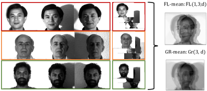
Figure 9: Averaging a collection of faces belonging to three different identities, captured under varying illumination: center, left and right. Notice that the first dimension of the flag representations is center illuminated, better representing the mean compared to Grassmannian.

E.2 Further Qualitative Results on MNIST

We use $20$ examples (e.g., points on $\mathcal{FL}(1,2;748)$) of $6$s and add $10$ examples of $7$s. We use the same workflow from the manuscript to represent the MNIST digits on $\mathrm{Gr}(2,748)$ and $\mathcal{FL}(1,2;748)$. We compute the averages on the Grassmannian [25, 45] and flag (ours). The reshaped first dimension of each of these averages is in Fig. 10. The brightness of the bottom left corner of each image is brighter the more present the $7$s digit (outlier class) is in the image. Notice the bottom left corner of each image, boxed in red, becomes darker as we move from left to right. So, our averaging on the flag is more robust to outliers than Grassmannian averaging. In fact, the bottom left corner of the flag-median is the darkest. Therefore, our flag-median is the least affected by the outlier examples of $7$s.

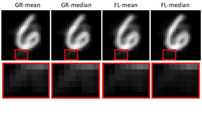
Figure 10: The first dimension of Grassmannian (“GR-”) and flag (“FL-”) averages of a data set with $20$ representations of $6$s and $10$ representations of $7$s. The bottom red boxes are the enlarged version of the upper image. Our flag-median is the least affected by the outlier examples of $7$s.

E.3 LBG Clustering on UFC YouTube

We use a subset of the UCF YouTube Action dataset [42] to run a similar experiment to what was done by Mankovich et al. [45]. The dataset contains labeled RGB video clips of people performing actions. Within each labeled action, the videos are grouped into subsets of clips with common features. We take approximately one example from each subset from each class. This results in $23$ examples of basketball shooting, $23$ of biking/cycling, $25$ of diving, $25$ of golf swinging, $24$ of horse back riding, $25$ of soccer juggling, $23$ of swinging, $24$ of tennis swinging, $24$ of trampoline jumping, 24 of volleyball spiking, and $24$ of walking with a dog. We convert these frames to gray scale, then we use INTER_AREA interpolation from the OpenCV package [16] to resize the frames to have only $450$ pixels. This is, on average, only $1\%$ of the number of pixels in the original frame. We vectorize and horizontally stack each video, then use the first $10$ columns of $\mathbf{Q}$ from the QR decomposition to realize each video as a point on $\mathrm{Gr}(10,450)$ and $\mathcal{FL}(1,2,\dots,10;450)$.

We run Linde-Buzo-Gray (LBG) clustering on these videos and report the resulting cluster purities in Fig. 11. Clustering on the flag manifold with our flag averages (blue boxes) improves cluster purities over Grassmannian methods. We also see higher variance in cluster purities for flag methods. Even though we are only working with approximately $1\%$ of the total number of pixels in each frame, we are able to produce cluster purities that are competitive with those reported in [45] using a similar set of videos. Specifically, our flag-LBG clustering is well within $0.1$ of the highest cluster purities reported in [45]. Overall, our flag methods improve cluster purities in a head-to-head experiment while remaining competitive with Grassmannian LBG with only using approximately 1% of pixels per frame.

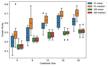
Figure 11: LBG cluster purities of YouTube videos with $10$ experiments with different numbers of centers, codebook sizes. The Grassmannian, e.g. “GR-”, boxes are results from LBG clustering using chordal distance and Grassmannian averages from [25, 45]. The “FL-” boxes are results from using the flag chordal distance and our flag-mean and -median.

E.4 Ablation Studies

Robustness to initialization

For Fig. 12, we fix a single-cluster dataset of $100$ points on $\mathcal{FL}(1,2,3;10)$ then run our IRLS algorithm for the flag-median and Stiefel RTR [2, 15] for the flag-mean with initial points that are further and further away from the center of the dataset. Our dataset is computed the same way we compute synthetic datasets for the manuscript: compute a center, $[\![\mathbf{C}]\!]\in\mathcal{FL}(1,2,3;10)$, and then add noise to the center using the parameter $\delta$. For this experiment we use $\delta=.2$. Our initial point for our IRLS algorithm and RTR is computed as the first $3$ columns of the QR decomposition of $\mathbf{C}+\mathbf{Z}\delta_{init}$ where $\mathbf{Z}\in\mathbb{R}^{10\times 3}$ has entries sampled from $\mathcal{U}[-.5,.5)$. We call $\delta_{init}$ the noise added to the initial point and plot it on the $x$-axis of Fig. 12. The “Error” is the chordal distance on $\mathcal{FL}(1,2,3;10)$ between the center and the algorithm output. “Iterations” is the number of iterations of RTR for the flag-mean and IRLS for the flag-median until convergence. “Cost” is the objective function values of the algorithm output. Our IRLS algorithm estimates the flag-median is further away from the center, $[\![\mathbf{C}]\!]$ than the flag-mean estimate. Also, the number of iterations of Stiefel RTR increases as we move the center further away from our dataset whereas our IRLS algorithm number of iterations remains constant. Finally, the cost value for the flag-median estimate is higher than the flag-mean estimate because the flag-mean estimate objective function likely contains squares of values less than $1$.

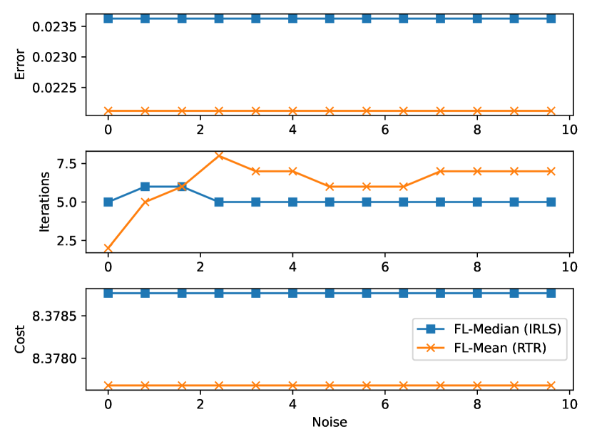
Figure 12: A plot of the robustness of our IRLS algorithm for the flag-median and Stiefel RTR for the flag-mean to initialization. For the median, we report the IRLS-iterations whereas for the mean, we report the RTR-iterations. Note that, even in large noise variances, both of the algorithms converge to a reasonable point regardless of initialization.

Computation time

We conducted the further experiments with ambient dimension and “dimension gap” and plot the runtime of Alg. 1 (Fl-Mean) and Alg. 2 (Fl-Median) in Fig. 13. As shown, the runtime increases linearly with dimension and decreases linearly with dimension gap. The FL-Mean is less affected than the FL-Median when changing $d$ or $d-k$. For high $d$, the runtime for the FL-Median is unstable with high standard deviation and high changes in the mean runtime across small changes in $d$. In contrast, the FL-Mean is relatively stable in run-time to increasing $d$. When we vary dimension gap ($d-k$), there is a negligible standard deviation in runtime for the FL-Mean and FL-Median. The FL-Median algorithm is very slow for low $d-k$ and as fast as the FL-Mean for high $d-k$. The FL-Mean algorithm runtime is more stable to changes in dimension gap than the FL-Median.

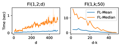
Figure 13: Time to compute the chordal flag-mean and -median of $10$ points over $20$ random trials. The shaded region is the standard deviation. We vary $d$ in $\mathcal{FL}(1,2;d)$ (left) and vary $d-k$ in $\mathcal{FL}(1,k;d=50)$ (right).

E.5 Motion Averaging

On error metrics

We score the quality of our averages using the geodesic distance on the pose manifold $SE(3)$ (or equivalently the geodesic distance on dual quaternions):

$$\epsilon(\mathbf{T}_{1},\mathbf{T}_{2})={\frac{1}{\pi}\|\log(\mathbf{R_{1}}^{\top}\mathbf{R}_{2})\|_{2}+\lambda_{T}\|\mathbf{t}_{1}-\mathbf{t}_{1}\|_{2}}$$ (36)

where $(\mathbf{R}_{i},\mathbf{t}_{i})$ are extracted from $\mathbf{T}_{i}$ as rotational and translational components, respectively. $\lambda_{T}$ is a scene dependent strictly positive scaling factor. Note that, as discussed in the paper, this is very much related to the $\lambda$ used in motion contraction. $\log(\cdot):SO(3)\to\mathfrak{so}(3)$ denotes the logarithmic map of the $SO(3)$-manifold. As such, this residual defined in Fig. 36 is equivalent to:

$$\epsilon(\mathbf{T}_{1},\mathbf{T}_{2})={\frac{1}{\pi}\arccos\left(\mathrm{tr}\frac{\mathbf{R}_{1}^{\top}\mathbf{R}_{2}-1}{2}\right)+\lambda_{s}\|\mathbf{t}_{1}-\mathbf{t}_{2}\|_{2}}.$$

Single rotation averaging

Single rotation averaging where a set of rotation matrices are averaged, is a special case of motion averaging where the translational components are set to zero. Due to the compactness of the manifold, additional $SO(3)$-specific averaging algorithms can be employed for the case of pure rotations. To compare our method against a larger class of well established, rotation-specific averaging algorithms we opt for zeroing the translational components, performing averages and reporting only the angular errors. Figs. 14,15 present our results with increasing noise and increasing outliers respectively. For the case of outliers, we further include the recent robust methods of Rie & Civera [40]. Naive refers to the Euclidean averages of rotation matrices (with a subsequent projection).

Impact of $\lambda$

As we have discussed in the paper, the scene-dependent scaling $\lambda$ is a hyper-parameter in our $SE(3)$-averaging. Note that, other distance metrics such as the ones dependent on 3D point distances exist [17]. These metrics exploit the action of 3D transformations on an auxiliary point set to measure distances in the 3D configuration of points. However, even those are somehow dependent upon a hyper-parameter such as the diameter of the point set or the point configurations. This is why we evaluate the impact of $\lambda$ in our averaging. In particular, we design multiple experiments to average $250$ random points on $SE(3)$ generated with an angular noise level of $0.075$. The radius of this scene is set to $1$, up to a translational noise level of $0.15$. This also means that the optimal $\lambda^{\star}$ (unknown during test) is $1$. We then vary $\lambda\in[0.002,0.025,0.1,0.25,0.5,0.75,1,1.25,1.5,1.8,2,2.25,\\ 2.5]$ and average $250$ random points, over $50$ runs. In each run, the point sets differ randomly. We compute the errors using Eq. E.5 with $\lambda=1$ and accumulate them over all runs. Fig. 16 plots the average errors per each $\lambda$. In this outlier-free regime, our flag-mean and flag-median are almost aligned when $\lambda=1$. Flag-median shows slight advantage over the mean for smaller values of $\lambda$.

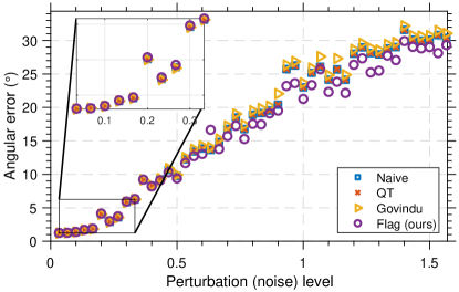
Figure 14: Single rotation averaging results for increasing levels of axial noise on synthetic, outlier-free data.

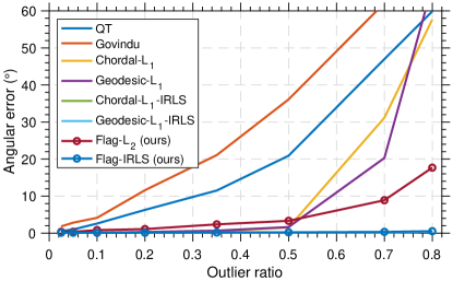
Figure 15: Single rotation averaging results for increasing levels of outliers on synthetic data with $<5^{\circ}$ of noise.

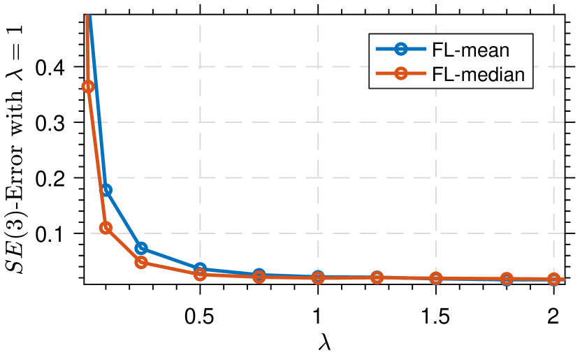
Figure 16: Impact of $\lambda$ our flag-mean and flag-median. During data generation we use $\lambda^{\star}=1$, whereas our algorithms use varying $\lambda$ as plotted in the $x$-axis. We then compare the resulting averages to the ground truth average and report the deviation. This is an outlier-free regime and as expected, median & mean prototypes overlap when we are at the optimal value, $\lambda=1$. Though, we also see that our algorithms are not too sensitive to the exact choice of this parameter.

Appendix F On Motion & Rotation Averaging

Motion averaging lies at the heart of structure from motion and 3D reconstruction in multi-view settings. Typically, the problem of recovering individual motions for a set of cameras when we are given a number of relative motion estimates between camera pairs is known as multiple motion averaging or transformation / motion synchronization [36, 8, 14, 22, 26, 21, 28, 29]. This problem is foundational for 3D structure recovery. Synchronization algorithms usually solve multiple single averaging sub-problems robustly [12, 41, 31], hence the name multiple motion averaging. These sub-problems involving the computation of a robust-barycenter of a set of points on $SE(3)$, are commonly known as robust single motion averaging and is the focus of our paper. Although our method directly operates on the product manifold, it is a de-facto standard to decompose the problem into single translation averaging and single rotation averaging. The lattter is particularly well studied due to the interesting mathematical structure of the problem [32, 31, 40, 29]. Nevertheless, our method is general enough to solve all of these variants, as we have experimented with in Figs. 14,15.

References

- [1] Rafal Ablamowicz, Garret Sobczyk, et al. Lectures on Clifford (geometric) algebras and applications. Springer, 2004.
- [2] P-A Absil, Christopher G Baker, and Kyle A Gallivan. Trust-region methods on Riemannian manifolds. Foundations of Computational Mathematics, 7(3):303–330, 2007.
- [3] Bijan Afsari. Riemannian center of mass: existence, uniqueness, and convexity. Proceedings of the American Mathematical Society, 139(2):655–673, 2011.
- [4] Khurrum Aftab and Richard Hartley. Convergence of iteratively re-weighted least squares to robust m-estimators. In 2015 IEEE Winter Conference on Applications of Computer Vision, pages 480–487. IEEE, 2015.
- [5] Khurrum Aftab, Richard Hartley, and Jochen Trumpf. Generalized weiszfeld algorithms for lq optimization. IEEE transactions on pattern analysis and machine intelligence, 37(4):728–745, 2014.
- [6] Giovanni Alberti. Geometric measure theory. Encyclopedia of mathematical Physics, 2:520–527, 2005.
- [7] DV Alekseevsky. Flag manifolds. Sbornik Radova, 11:3–35, 1997.
- [8] Federica Arrigoni, Beatrice Rossi, and Andrea Fusiello. Spectral synchronization of multiple views in SE(3). SIAM Journal on Imaging Sciences, 9(4):1963–1990, 2016.
- [9] Amir Beck and Shoham Sabach. Weiszfeld’s method: Old and new results. Journal of Optimization Theory and Applications, 164:1–40, 2015.
- [10] Peter N. Belhumeur, Joao P Hespanha, and David J. Kriegman. Eigenfaces vs. fisherfaces: recognition using class specific linear projection. IEEE Transactions on pattern analysis and machine intelligence, 19(7):711–720, 1997.
- [11] J Ross Beveridge, Bruce A Draper, Jen-Mei Chang, Michael Kirby, Holger Kley, and Chris Peterson. Principal angles separate subject illumination spaces in ydb and cmu-pie. IEEE transactions on pattern analysis and machine intelligence, 31(2):351–363, 2008.
- [12] Tolga Birdal, Michael Arbel, Umut Simsekli, and Leonidas J Guibas. Synchronizing probability measures on rotations via optimal transport. In IEEE/CVF Conference on Computer Vision and Pattern Recognition, 2020.
- [13] Tolga Birdal and Umut Simsekli. Probabilistic permutation synchronization using the riemannian structure of the birkhoff polytope. In Proceedings of the IEEE/CVF Conference on Computer Vision and Pattern Recognition, pages 11105–11116, 2019.
- [14] Tolga Birdal, Umut Simsekli, Mustafa Onur Eken, and Slobodan Ilic. Bayesian pose graph optimization via Bingham distributions and tempered geodesic MCMC. Advances in Neural Information Processing Systems, 31, 2018.
- [15] Nicolas Boumal, Bamdev Mishra, P-A Absil, and Rodolphe Sepulchre. Manopt, a Matlab toolbox for optimization on manifolds. The Journal of Machine Learning Research, 15(1):1455–1459, 2014.
- [16] G. Bradski. The OpenCV Library. Dr. Dobb’s Journal of Software Tools, 2000.
- [17] Romain Brégier, Frédéric Devernay, Laetitia Leyrit, and James L Crowley. Defining the pose of any 3d rigid object and an associated distance. International Journal of Computer Vision, 126(6):571–596, 2018.
- [18] Benjamin Busam, Tolga Birdal, and Nassir Navab. Camera pose filtering with local regression geodesics on the Riemannian manifold of dual quaternions. In IEEE International Conference on Computer Vision Workshop (ICCVW), October 2017.
- [19] Rudrasis Chakraborty, Soren Hauberg, and Baba C Vemuri. Intrinsic grassmann averages for online linear and robust subspace learning. In Proceedings of the IEEE Conference on Computer Vision and Pattern Recognition, pages 6196–6204, 2017.
- [20] Rudrasis Chakraborty and Baba C Vemuri. Recursive frechet mean computation on the grassmannian and its applications to computer vision. In Proceedings of the IEEE International Conference on Computer Vision, pages 4229–4237, 2015.
- [21] Avishek Chatterjee and Venu Madhav Govindu. Robust relative rotation averaging. IEEE transactions on pattern analysis and machine intelligence, 40(4):958–972, 2017.
- [22] Frank Dellaert, David M Rosen, Jing Wu, Robert Mahony, and Luca Carlone. Shonan rotation averaging: global optimality by surfing . In European Conference on Computer Vision, pages 292–308. Springer, 2020.
- [23] Li Deng. The MNIST database of handwritten digit images for machine learning research. IEEE signal processing magazine, 29(6):141–142, 2012.
- [24] Ron Donagi and Eric Sharpe. Glsms for partial flag manifolds. Journal of Geometry and Physics, 58(12):1662–1692, 2008.
- [25] Bruce Draper, Michael Kirby, Justin Marks, Tim Marrinan, and Chris Peterson. A flag representation for finite collections of subspaces of mixed dimensions. Linear Algebra and its Applications, 451:15–32, 2014.
- [26] Anders Eriksson, Carl Olsson, Fredrik Kahl, and Tat-Jun Chin. Rotation averaging with the chordal distance: Global minimizers and strong duality. IEEE Transactions of Pattern Analysis & Machine Intelligence (T-PAMI), 2019.
- [27] P Thomas Fletcher and Sarang Joshi. Riemannian geometry for the statistical analysis of diffusion tensor data. Signal Processing, 87(2):250–262, 2007.
- [28] Venu Madhav Govindu. Combining two-view constraints for motion estimation. In Proceedings of the IEEE Computer Society Conference on Computer Vision and Pattern Recognition (CVPR)., volume 2, pages II–II. IEEE, 2001.
- [29] Venu Madhav Govindu. Lie-algebraic averaging for globally consistent motion estimation. In Proceedings of the IEEE Computer Society Conference on Computer Vision and Pattern Recognition (CVPR), 2004., volume 1, pages I–I. IEEE, 2004.
- [30] Mehrtash T Harandi, Conrad Sanderson, Sareh Shirazi, and Brian C Lovell. Graph embedding discriminant analysis on grassmannian manifolds for improved image set matching. In CVPR 2011, pages 2705–2712. IEEE, 2011.
- [31] Richard Hartley, Khurrum Aftab, and Jochen Trumpf. L1 rotation averaging using the weiszfeld algorithm. In Proceedings of the IEEE/CVF Conference on Computer Vision and Pattern Recognition, 2011.
- [32] Richard Hartley, Jochen Trumpf, Yuchao Dai, and Hongdong Li. Rotation averaging. International journal of computer vision, 103(3):267–305, 2013.
- [33] Jun He, Laura Balzano, and Arthur Szlam. Incremental gradient on the grassmannian for online foreground and background separation in subsampled video. In 2012 IEEE Conference on Computer Vision and Pattern Recognition, pages 1568–1575. IEEE, 2012.
- [34] Yi Hong, Roland Kwitt, Nikhil Singh, Brad Davis, Nuno Vasconcelos, and Marc Niethammer. Geodesic regression on the grassmannian. In Computer Vision–ECCV 2014: 13th European Conference, Zurich, Switzerland, September 6-12, 2014, Proceedings, Part II 13, pages 632–646. Springer, 2014.
- [35] Harold Hotelling. Analysis of a complex of statistical variables into principal components. Journal of educational psychology, 24(6):417, 1933.
- [36] Xiangru Huang, Zhenxiao Liang, Xiaowei Zhou, Yao Xie, Leonidas J Guibas, and Qixing Huang. Learning transformation synchronization. In Proceedings of the IEEE/CVF Conference on Computer Vision and Pattern Recognition, pages 8082–8091, 2019.
- [37] Michael Kirby. Geometric data analysis: an empirical approach to dimensionality reduction and the study of patterns, volume 31. Wiley New York, 2001.
- [38] Joseph B Kruskal and Myron Wish. Multidimensional scaling, volume 11. Sage, 1978.
- [39] Sriram Kumar and Andreas Savakis. Robust domain adaptation on the l1-grassmannian manifold. In Proceedings of the IEEE Conference on Computer Vision and Pattern Recognition Workshops, pages 103–110, 2016.
- [40] Seong Hun Lee and Javier Civera. Robust single rotation averaging. arXiv preprint arXiv:2004.00732, 2020.
- [41] Xinyi Li and Haibin Ling. Hybrid camera pose estimation with online partitioning for slam. IEEE Robotics and Automation Letters, 5(2):1453–1460, 2020.
- [42] Jingen Liu, Jiebo Luo, and Mubarak Shah. Recognizing realistic actions from videos “in the wild”. In 2009 IEEE Conference on Computer Vision and Pattern Recognition, pages 1996–2003. IEEE, 2009.
- [43] Xiaofeng Ma, Michael Kirby, and Chris Peterson. The flag manifold as a tool for analyzing and comparing sets of data sets. In Proceedings of the IEEE/CVF International Conference on Computer Vision, pages 4185–4194, 2021.
- [44] Xiaofeng Ma, Michael Kirby, and Chris Peterson. Self-organizing mappings on the flag manifold with applications to hyper-spectral image data analysis. Neural Computing and Applications, 34(1):39–49, 2022.
- [45] Nathan Mankovich, Emily J King, Chris Peterson, and Michael Kirby. The flag median and FlagIRLS. In Proceedings of the IEEE/CVF Conference on Computer Vision and Pattern Recognition, pages 10339–10347, 2022.
- [46] F Landis Markley, Yang Cheng, John L Crassidis, and Yaakov Oshman. Averaging quaternions. Journal of Guidance, Control, and Dynamics, 30(4):1193–1197, 2007.
- [47] Timothy Marrinan, J Ross Beveridge, Bruce Draper, Michael Kirby, and Chris Peterson. Flag-based detection of weak gas signatures in long-wave infrared hyperspectral image sequences. In Algorithms and Technologies for Multispectral, Hyperspectral, and Ultraspectral Imagery XXII, volume 9840, pages 407–416. SPIE, 2016.
- [48] Tim Marrinan, J Ross Beveridge, Bruce Draper, Michael Kirby, and Chris Peterson. Finding the subspace mean or median to fit your need. In Proceedings of the IEEE Conference on Computer Vision and Pattern Recognition, pages 1082–1089, 2014.
- [49] Breton Lawrence Minnehan. Deep Grassmann Manifold Optimization for Computer Vision. Rochester Institute of Technology, 2019.
- [50] Georg Nawratil. Fundamentals of quaternionic kinematics in Euclidean 4-space. Advances in Applied Clifford Algebras, 26(2):693–717, 2016.
- [51] Du Nguyen. Closed-form geodesics and optimization for Riemannian logarithms of Stiefel and flag manifolds. Journal of Optimization Theory and Applications, pages 1–25, 2022.
- [52] Yasunori Nishimori, Shotaro Akaho, Samer Abdallah, and Mark D Plumbley. Flag manifolds for subspace ICA problems. In 2007 IEEE International Conference on Acoustics, Speech and Signal Processing-ICASSP’07, volume 4, pages IV–1417. IEEE, 2007.
- [53] Yasunori Nishimori, Shotaro Akaho, and Mark D Plumbley. Riemannian optimization method on generalized flag manifolds for complex and subspace ICA. In AIP Conference Proceedings, volume 872, pages 89–96. American Institute of Physics, 2006.
- [54] Yasunori Nishimori, Shotaro Akaho, and Mark D Plumbley. Riemannian optimization method on generalized flag manifolds for complex and subspace ica. In AIP Conference Proceedings, volume 872, pages 89–96. American Institute of Physics, 2006.
- [55] Yasunori Nishimori, Shotaro Akaho, and Mark D Plumbley. Riemannian optimization method on the flag manifold for independent subspace analysis. In International conference on independent component analysis and signal separation, pages 295–302. Springer, 2006.
- [56] Yasunori Nishimori, Shotaro Akaho, and Mark D Plumbley. Natural conjugate gradient on complex flag manifolds for complex independent subspace analysis. In International Conference on Artificial Neural Networks, pages 165–174. Springer, 2008.
- [57] Onur Ozyesil, Nir Sharon, and Amit Singer. Synchronization over Cartan motion groups via contraction. SIAM Journal on Applied Algebra and Geometry, 2(2):207–241, 2018.
- [58] Renaud-Alexandre Pitaval and Olav Tirkkonen. Flag orbit codes and their expansion to Stiefel codes. In 2013 IEEE Information Theory Workshop (ITW), pages 1–5. IEEE, 2013.
- [59] JM Selig. The study quadric. Geometric Fundamentals of Robotics, pages 241–269, 2005.
- [60] Andrea Torsello, Emanuele Rodola, and Andrea Albarelli. Multiview registration via graph diffusion of dual quaternions. In CVPR 2011, pages 2441–2448. IEEE, 2011.
- [61] Mark Wiggerman. The fundamental group of a real flag manifold. Indagationes Mathematicae, 9(1):141–153, 1998.
- [62] Wendy S Yambor. Analysis of PCA-based and Fisher discriminant-based image recognition algorithms. Master’s thesis, Citeseer, 2000.
- [63] Ke Ye, Ken Sze-Wai Wong, and Lek-Heng Lim. Optimization on flag manifolds. Mathematical Programming, 194(1):621–660, 2022.
- [64] Jiayao Zhang, Guangxu Zhu, Robert W Heath Jr, and Kaibin Huang. Grassmannian learning: Embedding geometry awareness in shallow and deep learning. arXiv preprint arXiv:1808.02229, 2018.
- [65] Yongheng Zhao, Tolga Birdal, Jan Eric Lenssen, Emanuele Menegatti, Leonidas Guibas, and Federico Tombari. Quaternion equivariant capsule networks for 3d point clouds. In Computer Vision–ECCV 2020: 16th European Conference, Glasgow, UK, August 23–28, 2020, Proceedings, Part I 16, pages 1–19. Springer, 2020.