Generalization with quantum geometry for learning unitaries

Abstract

Generalization is the ability of quantum machine learning models to make accurate predictions on new data by learning from training data. Here, we introduce the data quantum Fisher information metric (DQFIM) to determine when a model can generalize. For variational learning of unitaries, the DQFIM quantifies the amount of circuit parameters and training data needed to successfully train and generalize. We apply the DQFIM to explain when a constant number of training states and polynomial number of parameters are sufficient for generalization. Further, we can improve generalization by removing symmetries from training data. Finally, we show that out-of-distribution generalization, where training and testing data are drawn from different data distributions, can be better than using the same distribution. Our work opens up new approaches to improve generalization in quantum machine learning.

The key challenge in quantum machine learning is to design models that can learn from data and apply their acquired knowledge to perform well on new data [1]. This latter ability is called generalization and has been intensely studied recently [2, 3, 4, 5, 6, 7, 8, 9, 10, 11, 12, 13, 14, 15, 16, 17]. Constructing models that generalize well is essential for quantum machine learning tasks such as variational learning of unitaries [18, 19, 20, 21, 22, 23, 24], which is applied to unitary compiling [25, 26, 11], quantum simulation [27, 10, 28], quantum autoencoders [29, 30] and black-hole recovery protocols [31].

However, a priori it is difficult to predict whether a given quantum machine learning model will be able to generalize and usually time-consuming numerical studies have to be performed. This is further confounded by the fact that the training of quantum machine learning models is usually hard [32, 33, 34, 35, 36] and requires careful design to succeed [37, 33, 38, 32, 39].

Thus, a metric that quantitatively predicts both training success and generalization is essential to aid the quest for better quantum machine learning models [40, 41, 42, 43, 44, 45, 46, 47, 48, 49, 8] and potential advantages over classical models [50, 51, 52, 53]. In classical machine learning, measures of capacity have been developed which can directly evaluate generalization [54, 55, 56, 4, 5]. Recent works proposed the quantum Fisher information metric to measure the capacity of parameterized quantum states [48, 37, 57, 58], however a connection with generalization has not been established.

Here, we introduce the data quantum Fisher information metric (DQFIM) to predict the performance of quantum machine learning models for learning unitaries. Given an ansatz circuit and training data, the rank of the DQFIM quantifies the circuit depth and amount of data needed for generalization and convergence to a global minimum of the cost function. We apply the DQFIM to reduce the cost of generalization by finding models which require a low number of training data. Further, out-of-distribution generalization, i.e. the training data is drawn from a different distribution than the test data, can exhibit better performance compared to in-distribution generalization. Finally, while symmetries can reduce complexity, they can also hinder generalization. Our measure provides a practical way to understand the generalization capability of quantum machine learning models and guides the design of better models.

Model.—  Let us consider a target unitary $V$, which we want to approximate with ansatz unitary $U(\boldsymbol{\theta})$ parameterized by $M$-dimensional parameter vector $\boldsymbol{\theta}$. We learn from a training set $S_{L}=\{|\psi_{\ell}\rangle,V|\psi_{\ell}\rangle\}_{\ell=1}^{L}$ of $L$ states which are randomly drawn from a distribution of states $|\psi_{\ell}\rangle\in W$ [59, 10, 28]. We learn by minimizing the cost function given by the fidelity

$$C_{\text{train}}(\boldsymbol{\theta},S_{L})=1-\frac{1}{L}\sum_{\ell=1}^{L}|\langle\psi_{\ell}|V^{\dagger}U(\boldsymbol{\theta})|\psi_{\ell}\rangle|^{2}\,,$$ (1)

which can be efficiently measured with the SWAP test [60]. This model generalizes when the learned unitary correctly transforms any state sampled from $W$ which is evaluated with the test error

$$C_{\text{test}}(\boldsymbol{\theta},W)=1-\underset{|\psi\rangle\in W}{\mathbb{E}}[|\langle\psi|V^{\dagger}U(\boldsymbol{\theta})|\psi\rangle|^{2}]\,.$$ (2)

In variational quantum algorithms [20] and quantum control [61], the parameterized ansatz unitary $U(\boldsymbol{\theta})=\prod_{k=1}^{G}U^{(k)}(\boldsymbol{\theta}_{k})$ commonly consists of $G$ repeating layers of unitaries $U^{(k)}(\boldsymbol{\theta}_{k})=\prod_{n=1}^{K}\exp(-i\theta_{kn}H_{n})$, where $H_{n}$ are hermitian operators, $\boldsymbol{\theta}_{k}$ a $K$-dimensional vector, and $\boldsymbol{\theta}=\{\boldsymbol{\theta}_{1},\dots,\boldsymbol{\theta}_{G}\}$ the $M=GK$ dimensional parameter vector. The optimization program starts with a randomly chosen $\boldsymbol{\theta}$ and iteratively minimizes Eq. (1) with the gradient $\nabla C_{\text{train}}(\boldsymbol{\theta})$, which can be efficiently estimated by a quantum computer [62]. Gradient descent iteratively updates $\boldsymbol{\theta}\rightarrow\boldsymbol{\theta}-\alpha\nabla C_{\text{train}}$ with some $\alpha$ until reaching a minimum after $E$ training steps, where $\nabla C_{\text{train}}(\boldsymbol{\theta}^{*})=0$ with parameter $\boldsymbol{\theta}^{*}$. We assume that ansatz $U(\boldsymbol{\theta})$ can represent the target unitary $V$, i.e. there is a parameter $\boldsymbol{\theta}_{\text{g}}$ such that $C_{\text{test}}(\boldsymbol{\theta}_{\text{g}},W)=C_{\text{train}}(\boldsymbol{\theta}_{\text{g}},S_{L})=0$, which we enforce by choosing $V=U(\boldsymbol{\theta}_{\text{g}})$ with a randomly selected $\boldsymbol{\theta}_{\text{g}}$.

After training we have three possible outcomes: $(i)$ Reach a local minimum $C_{\text{train}}(\boldsymbol{\theta}^{*},S_{L})>0$, $C_{\text{test}}(\boldsymbol{\theta}^{*},S_{L})>0$ with an incorrect unitary for both training set $S_{L}$ and distribution $W$; $(ii)$ Reach global minimum $C_{\text{train}}(\boldsymbol{\theta}^{*},S_{L})=0$, however no generalization with $C_{\text{test}}(\boldsymbol{\theta}^{*},W)>0$. Here, $U(\boldsymbol{\theta}^{*})$ correctly transform $S_{L}$, but performs poorly on states from $W$. $(iii)$ Achieve global minimum and generalization with $C_{\text{train}}(\boldsymbol{\theta}^{*},S_{L})=C_{\text{test}}(\boldsymbol{\theta}^{*},W)=0$ for any state from $W$. In the following, we show that the DQFIM determines the critical number of circuit parameters $M_{\text{c}}$ and training states $L_{\text{c}}$ required to reach the global minimum and generalization which is the main result of our work.

 

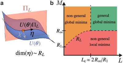
Figure 1: a) We represent unitary $V$ with ansatz unitary $U(\boldsymbol{\theta})$ by optimizing the $M$-dimensional parameter vector $\boldsymbol{\theta}$ in respect to cost function Eq. (1) using $L$ training states $S_{L}=\{|\psi_{\ell}\rangle,V|\psi_{\ell}\rangle\}_{\ell=1}^{L}$. Only the isometry $U(\boldsymbol{\theta})\Pi_{L}$ can be learned, where $\Pi_{L}$ is the projector onto the space spanned by $\{|\psi_{\ell}\rangle\}_{\ell=1}^{L}$. The maximal rank of the data quantum Fisher information metric (DQFIM) $R_{L}$ describes the degrees of freedom of $U(\boldsymbol{\theta})\Pi_{L}$ that can be learned with $L$ training states. b) Phase diagram of optimisation and generalization with $M$ and $L$. Convergence to global minimum ($C_{\text{train}}\approx 0)$ is likely when $M\geq R_{L}$. The trained unitary can generalize to unseen test data ($C_{\text{test}}\approx 0$) for $L\geq L_{\text{c}}\approx 2R_{\infty}/R_{1}$ and $M\geq R_{\infty}$.

DQFIM.—  A given training set $S_{L}$ allows us to learn a part of the unitary $U(\boldsymbol{\theta})$, which we define as follows:

Definition 1 (Learnable isometry).

Given training set $S_{L}=\{|\psi_{\ell}\rangle,V|\psi_{\ell}\rangle\}_{\ell=1}^{L}$ of $L$ states, we define projector $\Pi_{L}$ onto the space spanned by the states $\{|\psi_{\ell}\rangle\}_{\ell=1}^{L}$ and its normalization $\tilde{\Pi}_{L}$

$$\Pi_{L}=\sum_{k=1}^{B_{L}}|\phi_{k}\rangle\langle\phi_{k}|\,;\,\,\,\tilde{\Pi}_{L}=\Pi_{L}/B_{L}$$ (3)

where $|\phi_{k}\rangle$ are the eigenvectors with non-zero eigenvalue of $\rho_{L}=L^{-1}\sum_{\ell=1}^{L}|\psi_{\ell}\rangle\langle\psi_{\ell}|$ and $B_{L}=\mathrm{rank}(\rho_{L})$. Training with cost function Eq. (1) learns the projection of the unitary $U(\boldsymbol{\theta})$ onto $\Pi_{L}$, which is the isometry

$$U_{L}(\boldsymbol{\theta})=U(\boldsymbol{\theta})\Pi_{L}\,.$$ (4)

To understand Eq. (4), let us consider the $d$-dimensional unitary $U\equiv U(\boldsymbol{u})=\sum_{n,k=1}^{d}u_{nk}|n\rangle\langle k|$ with complex parameters $\boldsymbol{u}=\{u_{11},u_{12},\dots,u_{dd}\}$ and training set $S_{L}=\{|\ell\rangle,V|\ell\rangle\}_{\ell=1}^{L}$, where $|\ell\rangle\in W_{\text{comp}}$ are computational basis states and $V$ some unitary. For $L=1$, training with Eq. (1) optimizes $U|1\rangle=\sum_{n=1}^{d}u_{n1}|n\rangle$. Here, only the parameters of the column vector $u_{1}=(u_{11},u_{21},\dots,u_{d1})$ of $U$ have an effect on the state and can be learned, while all other parameters are hidden. For any $L$, applying $U$ on the states of $S_{L}$ gives us $\{U|\ell\rangle=\sum_{n=1}^{d}u_{n\ell}|n\rangle\}_{\ell=1}^{L}$. The learnable parameters of $U$ correspond to the $d\times L$-dimensional isometry $U_{L}=(u_{1},\dots,u_{L})\equiv U\Pi_{L}$ with projector $\Pi_{L}=\sum_{\ell=1}^{L}|\ell\rangle\langle\ell|$ and $U_{L}^{\dagger}U_{L}=\Pi_{L}$ (see Fig. 1a). Even if we find a global minima with $C_{\text{train}}=0$, training set $S_{L}$ with $L<d$ provides no information about the column vectors $(u_{L+1},\dots,u_{d})$. The trained model $U(\boldsymbol{u}^{*})$ will randomly guess these column vectors, resulting in generalization error $C_{\text{test}}>0$. Only for $L=d$, we have a complete training set that can achieve generalization $C_{\text{test}}=0$.

We can understand generalization with the number of independent parameters (or effective dimension) $D_{L}$ of the isometry $U_{L}$. For $L=1$, $U|1\rangle=\sum_{n=1}^{d}u_{n1}|n\rangle=\sum_{n=1}^{d}(a_{n1}+ib_{n1})|n\rangle$ has $2d$ real parameters $a_{n1}$, $b_{n1}$. However, due to global phase and norm, there are only $D_{1}=2d-2$ independent parameters. For $L=d$, parameterizing a complete unitary $U$ requires $D_{d}=d^{2}-1$ parameters. For example, a single qubit has $D_{1}=2$ (Bloch sphere) and $D_{2}=3$ (arbitrary unitary) free parameters [63], and thus we require $L\geq 2$ states to generalize. However, depending on ansatz and data there can be less independent parameters $D_{L}$. Let us consider $U(\theta_{1},\theta_{2})=\exp(-i\sigma_{z}\theta_{1})\exp(-i\sigma_{z}\theta_{2})$ and distribution $\{|+\rangle,|-\rangle\}$ with $|+\rangle=\frac{1}{\sqrt{2}}(|0\rangle\pm|1\rangle)$ and $z$-Pauli $\sigma_{z}$. While we have $M=2$ parameters, the generators commute and there is only $D_{1}=D_{d}=1$ independent parameter and $L=1$ state is already sufficient to generalize. In contrast, for distribution $\{|0\rangle,|1\rangle\}$ we have $D_{L}=0$ and $L=0$ as only the global phase is rotated.

For general $S_{L}$ and $U(\boldsymbol{\theta})$, we now propose the DQFIM to quantify the effective dimension that can be learned (see Supplemental materials (SM) E for derivation):

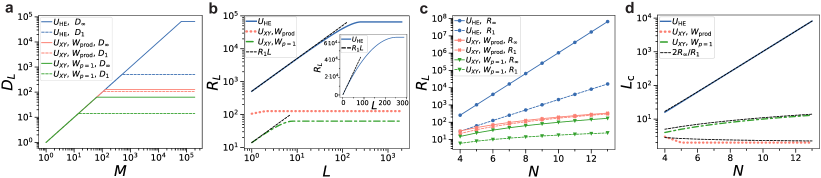
Figure 2: DQFIM for different unitaries $U$ with $M$ parameters and $L$ training states. As defined in SM A, we show hardware efficient circuit $U_{\text{HE}}$ with no symmetries and Haar random training states (blue curves), as well as $U_{XY}$ with particle number symmetry using as training data either product states $W_{\text{prod}}$ (orange) or symmetry-conserving states $W_{p=1}$ (green). a) Effective dimension $D_{L}$ increases linearly with $M$, until it reaches a maximal value $R_{L}$ for $M\geq M_{\text{c}}(L)$. We have $N=8$ qubits. b) $R_{L}$ increases with $L$ until converging to $R_{\infty}$ for $L\geq L_{\text{c}}$. Black dashed line shows approximation $R_{L}\sim R_{1}L$. Inset shows generic ansatz without log-plot, highlighting the non-linear behavior of $R_{L}$. c) Scaling of $R_{1}$ and $R_{\infty}$ with qubit number $N$. d) Number $L_{\text{c}}$ of training states needed for generalization. Black dashed line shows $L_{\text{c}}\approx 2R_{\infty}/R_{1}$.

Definition 2 (DQFIM).

For unitary $U(\boldsymbol{\theta})$ and training set $S_{L}$, the DQFIM is defined as

$$\mathcal{Q}_{nm}(S_{L},U(\boldsymbol{\theta}))=$$ (5)

$$4\mathrm{Re}(\mathrm{tr}(\partial_{n}U^{\dagger}\tilde{\Pi}_{L}\partial_{m}U)-\mathrm{tr}(\partial_{n}U^{\dagger}\tilde{\Pi}_{L}U)\mathrm{tr}(U^{\dagger}\tilde{\Pi}_{L}\partial_{m}U))$$

where $\partial_{n}$ is the derivative in respect to the $n$th entry of the $M$-dimensional vector $\boldsymbol{\theta}=(\theta_{1},\dots,\theta_{M})$ and $\tilde{\Pi}_{L}$ is given by Eq. (3). We also define the effective dimension

$$D_{L}(S_{L},U(\boldsymbol{\theta}))=\mathrm{rank}(\mathcal{Q}(S_{L},U(\boldsymbol{\theta}))\leq M\,.$$ (6)

Intuitively, $\mathcal{Q}(S_{L},U(\boldsymbol{\theta}))$ is a metric that describes how a variation in $\boldsymbol{\theta}$ changes the isometry $U(\boldsymbol{\theta})\Pi_{L}$. For $L=1$, we recover the QFIM $\mathcal{F}_{nm}=4\text{Re}(\langle\partial_{n}\psi|\partial_{m}\psi\rangle-\langle\partial_{n}\psi|\psi\rangle\langle\psi|\partial_{m}\psi\rangle)$ [64, 57], where $D_{1}$ describes the effective dimension that a parameterized state $U(\boldsymbol{\theta})|\psi_{1}\rangle$ can explore [48]. $D_{1}$ increases when adding more layers $G$ and thus parameters $M$ to $U(\boldsymbol{\theta})$, until reaching a maximal value $R_{1}$ (see Fig. 2a). Here, the state $U(\boldsymbol{\theta})|\psi_{1}\rangle$ is overparameterized as it can explore all possible degrees of freedom of the ansatz for $L=1$ [37]. Similarly, we introduce $R_{L}$ to describe the maximal number of degrees of freedom that the isometry $U_{L}$ can explore for any $L$:

Definition 3 (Overparameterization).

Ansatz $U(\boldsymbol{\theta},M)$ with training set $S_{L}$ is overparameterized when effective dimension $D_{L}$ does not increase further upon increasing the number of parameters $M$. The maximal rank $R_{L}$ reached for $M\geq M_{\text{c}}(L)$ is given by

$$R_{L}\equiv\max_{M\geq M_{\text{c}}(L),\boldsymbol{\theta}}D_{L}(S_{L},U(\boldsymbol{\theta},M))\,.$$ (7)

Once $M\geq M_{\text{c}}(L)$, a variation of $\boldsymbol{\theta}$ can explore all degrees of freedom of $U_{L}$. Thus, minimization is unlikely to get stuck in a local minimum of cost function $C_{\text{train}}$ [65, 66, 32, 38, 37].

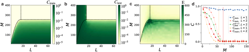
Figure 3: a) $C_{\text{train}}$ against $M$ and $L$. Dashed black lines indicate $M_{\text{c}}(L)=R_{L}$ and $L_{\text{c}}=2R_{\infty}/R_{1}$. We have a $N=4$ qubit hardware-efficient ansatz with Haar random training states, where we initialize with a random parameter, train with a gradient descent algorithm [67] simulated with [68] and average over 10 training repetitions. Target unitary is chosen as $V=U(\boldsymbol{\theta}_{\text{g}})$, where $\boldsymbol{\theta}_{\text{g}}$ is a random parameter of the ansatz unitary. b) Average $C_{\text{test}}$ against $M$ and $L$. c) Number of training steps $E$ until reaching $C_{\text{train}}<10^{-4}$. d) $C_{\text{test}}$ and $C_{\text{train}}$ against $M$ with $U_{XY}$ ansatz for $N=6$ qubits, where we train with $L=1$ and $L=2$ product states $W_{\mathrm{prod}}$. We use $W_{\mathrm{prod}}$ as test states, except for green dotted curve $C_{\text{test}}^{p=1}$ where we show out-of-distribution generalization with symmetric test states $W_{p=1}$. The dashed vertical lines indicate $R_{1}$ (yellow) and $R_{2}$ (red).

Observation 1 (Convergence to global minima).

Global minimum $C_{\text{train}}(\boldsymbol{\theta}^{*})\approx 0$ with training set $S_{L}$ is reached with high probability when $M\geq M_{\text{c}}(L)\geq R_{L}$.

As seen in Fig. 2b, $R_{L}$ and thus the circuit parameters needed to reach the global minimum increases with $L$, where the growth slows down due to unitary constraints. We find the upper bound (SM F or [69])

$$R_{L}\leq 2dL-L^{2}-1\,\,\mathrm{for}\,L\leq d\,;\,\,R_{L}\leq d^{2}-1\,\,\mathrm{for}\,\,L>d\,.$$ (8)

Once the maximal possible $R_{L}$ is reached, the training states are sufficient to learn all degrees of freedom of $U$. Thus, we have an overcomplete training set:

Definition 4 (Overcomplete data for learning unitaries).

For a given ansatz $U$, training set $S_{L}$ of $L$ training states $|\psi_{\ell}\rangle\in W$ drawn from ensemble $W$ is overcomplete when $R_{L}$ does not increase further upon increase of $L$. The maximal rank $R_{\infty}$ is reached for $L_{\text{c}}$ training states

$$R_{\infty}=R_{L_{\text{c}}}(W,U)\equiv\max_{L\geq L_{\text{c}}}\underset{|\psi_{\ell}\rangle\in W}{\mathbb{E}}[R_{L}(S_{L},U)]\,.$$ (9)

We bound $R_{L}$ similar to $R_{1}$ for Ref. [37] (see SM G):

Theorem 1.

The maximal rank $R_{L}$ is bounded by the dimension of the dynamical Lie algebra (DLA)

$$R_{L}\leq\dim(\mathfrak{g})\,,$$ (10)

where $\mathfrak{g}=\mathrm{span}\left\langle iH_{1},\ldots,iH_{K}\right\rangle_{\text{Lie}}$ is generated by the repeated nested commutators of the generators $H_{k}$ of $U(\boldsymbol{\theta})$.

By choosing the training states on the support of the DLA, we can find an overcomplete training set with $L_{\text{c}}\leq\text{dim}(\mathfrak{g})$. In particular, when $\text{dim}(\mathfrak{g})\sim\text{poly}(N)$ we have $L_{\text{c}}\sim\text{poly}(N)$ and $M_{\text{c}}\sim\text{poly}(N)$.

We can estimate $L_{\text{c}}$ with the following consideration: To generalize we have to learn all $R_{\infty}$ degrees of freedom of the unitary. The first training state allows us to learn $R_{1}$ degrees of freedom, while each additional state provides a bit less as seen in Eq. (8). For the upper bound Eq. (8) we have $L_{\text{c}}\approx 2R_{\infty}/R_{1}$, which we numerically find to be a good estimation also for other models:

Observation 2 (Generalization for learning unitaries).

A trained model generalizes $C_{\text{test}}(\boldsymbol{\theta}^{*})\approx 0$ with high probability when the model is overparameterized (i.e. $M\geq M_{\text{c}}\geq R_{L}$ for Def. 3) and overcomplete (i.e. $L\geq L_{\text{c}}$ for Def. 4). The critical number of training states $L_{\text{c}}$ needed to generalize can be approximated by

$$L_{\text{c}}\approx 2R_{\infty}/R_{1}\,.$$ (11)

Applications.—  We want to learn the unitary evolution $V_{XY}=\exp(-iH_{XY}t)$ in time $t$ of the XY-Hamiltonian $H_{XY}=\sum_{k=1}^{N}(\sigma_{k}^{x}\sigma_{k+1}^{x}+\sigma_{k}^{y}\sigma_{k+1}^{y}+h_{k}\sigma_{k}^{z})$, where $\sigma^{\alpha}_{k}$, $\alpha\in\{x,y,z\}$ is the Pauli operator acting on qubit $k$ and $h_{k}\in\mathbb{R}$. We learn $V_{XY}$ with the $U_{XY}(\boldsymbol{\theta})$ ansatz (see SM A), which can represent $V_{XY}$ with a polynomially number of parameters [70]. Further, $H_{XY}$ and $U_{XY}$ are symmetric in respect to the particle number operator $P=\sum_{k=1}^{N}\frac{1}{2}(1+\sigma^{z}_{k})$ with $[U_{XY},P]=[H_{XY},P]=0$, where $[.]$ is the commutator. We define the distribution $W_{p=1}$ of states $|\psi_{\ell}\rangle$ which are symmetric in regards to $P$, i.e. $P|\psi_{\ell}\rangle=|\psi_{\ell}\rangle$ with the same eigenvalue $p=1$ for all $\ell$. Further, we define the distribution of single-qubit product states $W_{\text{prod}}$ where $|\psi_{\ell}\rangle=\bigotimes_{k=1}^{N}|\phi^{k}_{\ell}\rangle,\,|\phi^{k}_{\ell}\rangle\in\mathcal{H}(\mathbb{C}^{2})$ which do not respect particle symmetry in general. We now study generalization with $U_{XY}$ depending on the symmetry of the training states:

Observation 3 (Generalization requires more data with symmetries).

Ansatz $U_{\text{XY}}$ conserves particle number operator $P$ with $[U_{\text{XY}},P]=0$. We learn with $(i)$ the ensemble of particle-number conserving states $|\psi_{\ell}\rangle\in W_{p=1}$ and $(ii)$ single-qubit product states $|\psi_{\ell}\rangle\in W_{\text{prod}}$. We generalize with $L\geq L_{\text{c}}$ training states where

$$(i)\;L_{\text{c}}= N\;\mathrm{for}\;|\psi_{\ell}\rangle\in W_{p=1}$$

$$(ii)\;L_{\text{c}}= 2\;\;\mathrm{for}\;|\psi_{\ell}\rangle\in W_{\mathrm{prod}}\,\,,N>4\,.$$

This result follows directly from the scaling of $R_{L}$ (see Fig. 2c,d). In particular, for $W_{p=1}$ we have $R_{1}=2N-2$, $R_{\infty}=N^{2}-1$, while for $W_{\mathrm{prod}}$ we find via numerical extrapolation $R_{1}=2N^{2}-3N+2$ and $R_{\infty}=2N^{2}-1$. Generalization improves without symmetries as $R_{1}$ grows larger for $p>1$ and thus product states with support on all $p$ gain more information about $U_{XY}$ than data restricted to $p=1$.

Next, we consider out-of-distribution generalization where one generates the training set from a different ensemble than the test states [8]:

Observation 4 (Out-of-distribution generalization requires less data).

Training $U_{XY}$ with $L\geq 2$ product states $|\psi_{\ell}\rangle\in W_{\mathrm{prod}}$ out-of-distribution generalizes symmetry conserving data $W_{p=1}$ with $C_{\mathrm{test}}(\boldsymbol{\theta}^{*},W_{\mathrm{prod}})=C_{\mathrm{test}}(\boldsymbol{\theta}^{*},W_{p=1})=0$. In contrast, training $U_{XY}$ with $|\psi_{\ell}\rangle\in W_{p=1}$ requires $L\geq N$ training states to achieve $C_{\mathrm{test}}(\boldsymbol{\theta}^{*},W_{p=1})=0$.

Numerical results.—  In Fig. 3a-c we study training for hardware-efficient ansatz $U_{\text{HE}}$ (see SM A). In Fig. 3a, we converge to local minima with $C_{\text{train}}\gg 0$ for $M\leq R_{L}$, while we find global minimum $C_{\text{train}}\approx 0$ for $M\geq R_{L}$, which is indicated as black dashed line. In Fig. 3b, generalization $C_{\text{test}}\approx 0$ is achieved only for $M\geq R_{\infty}$ and $L\geq L_{\text{c}}\approx 2R_{\infty}/R_{1}$ indicated by the vertical black lines. In Fig. 3c, the number of training steps $E$ needed to converge show characteristic peaks close to $M_{\text{c}}$ and $L_{\text{c}}$ indicated by black dashed lines. In Fig. 3d we study test and training error for the $U_{XY}$ ansatz for training with product state ensemble $W_{\mathrm{prod}}$. For sufficient $M$, we have $C_{\text{train}}\approx 0$ for $L=1$ and $L=2$ training data. Generalization with $C_{\text{test}}\approx 0$ requires $L\geq 2$ when testing in-distribution $W_{\mathrm{prod}}$ or out-of-distribution $W_{p=1}$. We study other models which generalize for constant $L$ in SM J and I.

In Fig. 4a we study $C_{\text{test}}$ against $L$, $M$ for $U_{XY}$ when training with particle-conserved ensemble $W_{p=1}$ (see also SM C). Generalization improves with $M$ and $L$, where the lower bound $C_{\text{test}}\sim 1-(L/L_{\text{c}})^{2}$ [6] is saturated for $M\geq M_{\text{c}}$. In Fig. 4b, we show that the training steps needed for convergence scale as $E\sim N^{2}$ with a clear peak at $L\approx L_{\text{c}}$ when overparameterized.

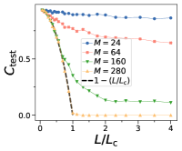
 a  b

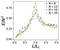
Figure 4: Learning with $U_{XY}$ and particle conserved data $|\psi_{\ell}\rangle\in W_{p=1}$. a) $C_{\text{test}}$ against $L$ for different $M$ with $N=16$, $L_{\text{c}}=N$. Black dashed line is $C_{\text{test}}\sim 1-(L/L_{\text{c}})^{2}$. b) Training steps $E$ needed to converge to $C_{\text{train}}<10^{-4}$ against $L$ for $M\gg M_{\text{c}}$.

Conclusion.—  The newly introduced DQFIM $\mathcal{Q}$ and its maximal rank $R_{L}$ tell us the amount of data $L$ and circuit parameters $M$ needed to successfully learn unitaries. Overparameterized models [37, 38, 32] converge to a global minimum with high probability for $M\geq M_{\text{c}}\geq R_{L}$. Generalization, i.e. correctly predicting new data, requires a critical number of training states $L\geq L_{\text{c}}$, which depends on the ratio $L_{\text{c}}\approx 2R_{\infty}/R_{1}$. Overparameterization and generalization appear in three distinct regimes, where training time increases substantially at the transitions, which could indicate a computational phase transition [24, 32]. While the complexity of unitaries grows linearly with $M$ [71, 48], the growth in learnable degrees of freedom $R_{L}$ and thus the circuit depth needed for overparameterization slows down with $L$. Generalization for overparameterized models scales as $C_{\text{test}}\sim 1-(L/L_{\text{c}})^{2}$ saturating the lower bound of Ref. [6], which is substantially better than the upper bound $C_{\text{test}}\sim\sqrt{1/L}$ [59, 7]. For underparameterized models the empirical risk $C_{\text{test}}-C_{\text{train}}$ [59] can insufficiently characterize generalization due to convergence to bad local minima (see SM B).

We show that generalization and overparameterization can be achieved with polynomial circuit depth and dataset size when the dimension of the DLA scales polynomially with $N$. When $R_{1}\sim N^{\gamma}$, $R_{\infty}\sim N^{\gamma}$ scale with the same $\gamma$, then $O(1)$ training states are sufficient to generalize, explaining the numerical observations of Ref. [10] (see also SM I). While symmetries can improve generalization [44, 45], we show that symmetries in data can also hinder generalization by increasing the $R_{\infty}/R_{1}$ ratio. Generalization improves here as symmetry-broken data has access to information of other symmetry sectors. This feature also allows out-of-distribution generalization [8] to outperform in-distribution generalization. Note that symmetry-broken data requires slightly more parameters, which implies an interesting trade-off between dataset size and circuit depth. Finally, the DQFIM could be extended to evaluate generalization for other quantum machine learning tasks [20] as well as data re-uploading  [72, 73], kernel models [74, 75] and the effect of noise [58]. The code for this work is available online [76].

Appendix A Ansatz unitaries

The ansatz unitaries used in the maint text are shown in Fig. 5. We assume that the considered unitaries have a periodic structure of $G$ layers with

$$U(\boldsymbol{\theta})=\prod_{k=1}^{G}U_{k}(\boldsymbol{\theta}_{k})\,,\,\,U^{(k)}(\theta_{k})=\prod_{n=1}^{K}\exp(-i\theta_{kn}H_{n})$$ (12)

where $U^{(k)}(\theta_{k})$ is the unitary of the $k$th layer. Here, $H_{n}$ are $K$ hermitian matrices and $\boldsymbol{\theta}_{k}=\{\theta_{k1},\dots,\theta_{kn}\}$ are the parameters of the $k$th layer. The total parameter vector $\theta=\{\boldsymbol{\theta}_{1},\dots,\boldsymbol{\theta}_{G}\}$ of the ansatz has $M=GK$ parameters.

In Fig.5a, we show a hard-ware efficient ansatz $U_{\text{HE}}$, which produces highly random circuits which span the full Hilbertspace nearly uniformly and are known to be hard to simulate classically. Overparameterization requires for this circuit exponentially many parameters.

 

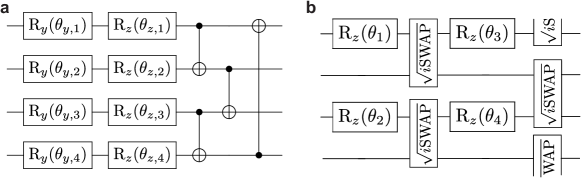
Figure 5: Ansatz unitaries for the main text. The circuits are repeated for $G$ layers. a) Hardware-efficient ansatz $U_{\text{HE}}$ consisting of parameterized $y$, $z$ rotations and CNOT gates. Has no symmetries and can realize arbitrary $N$-qubit unitaries for sufficient depth. b) $U_{XY}$ circuit inspired by $XY$-model Eq. (13). Composed of single qubit $z$ rotations and nearest-neighbor $\sqrt{\text{iSWAP}}$ gates, arranged with periodic boundary condition. Commutes with particle number operator $P$ and for sufficient depth can realize any time evolution generated by $\exp(-iH_{XY}t)$. c) Real-valued ansatz $U_{\text{Y-CZ}}$ consisting of $y$-rotations and control-$Z$ gates in a nearest-neighbor chain configuration.

In Fig.5b, we show an ansatz $U_{\text{XY}}$ with symmetries that overparameterizes in polynomial depth. This ansatz is inspired from the integrable XY Hamiltonian with random field $h_{k}$

$$H_{XY}=\sum_{k=1}^{N}h_{k}\sigma_{k}^{z}+\sum_{k=1}^{N}(\sigma_{k}^{x}\sigma_{k+1}^{x}+\sigma_{k}^{y}\sigma_{k+1}^{y})$$ (13)

$H_{XY}$ commutes with the particle number operator $P=\sum_{k=1}^{N}\frac{1}{2}(1+\sigma^{z}_{k})$ where $\sigma^{z}_{k}$ is the Pauli $z$ operator acting on qubit $k$. In particular, we have $[H_{XY},P]$. Time evolution $U=\exp(-iH_{XY}t)$ also conserves the symmetry, i.e. $[U,P]=0$. The ansatz $U_{XY}$ shown in 5b can represent the time evolution of the Hamiltonian. $U_{XY}$ consists of parameterized $z$-rotations and nearest-neighbor $\sqrt{\text{iSWAP}}=\exp(i\pi/8(\sigma_{k}^{x}\sigma_{k+1}^{x}+\sigma_{k}^{y}\sigma_{k+1}^{y}))$ gates. One can think of this model similar to a Trotterized version of the time evolution $U=\exp(-iH_{XY}t)$. The generators of $U_{XY}$ are the Pauli operators of $H_{XY}$. Thus, the time-evolution operator $U_{XY}$ spans the same dynamical Lie algebra as the time evolution generated by $H_{\text{XY}}$ and can represent any time evolution of $H_{\text{XY}}$ [70]. The dimension of the dynamical Lie-algebra spanned by $U_{XY}$ scales polynomial with qubit number $N$ and thus can be overparameterized with polynomially many parameters $M$ [37]. For random product states $W_{\text{prod}}$ as training set, we we find via numerical extrapolation $R_{1}=2N^{2}-3N+2$ and $R_{\infty}=2N^{2}-1$. We also choose a training set $W_{p=1}$ with $P=1$ particles, which consists of arbitrary superpositions of permutations of the basis states $|10\dots 0\rangle$. We have $P|\psi_{\ell}\rangle=|\psi_{\ell}\rangle$ for any state $|\psi_{\ell}\rangle\in W_{p=1}$. These states live in an effective $N$-dimensional subspace, yielding $R_{1}=2N-2$ and $R_{\infty}=N^{2}-1$.

Appendix B Generalization and empirical risk

We define generalization via the error of the cost function $C_{\text{test}}$ averages over the full data ensemble $W$. In our studies, we choose the problem such that $C_{\text{test}}=0$ can be achieved for at least one parameter $\boldsymbol{\theta}_{\text{g}}$.

In general, the minimal achievable $C_{\text{test}}$ for given ansatz and data distribution may not be known. Thus, often the empirical risk $\zeta=C_{\text{test}}-C_{\text{train}}$ of the trained model is used as a proxy to evaluate generalization [59]. In Fig. 6, we compare $C_{\text{train}}$, $C_{\text{test}}$ and empirical risk $C_{\text{test}}-C_{\text{train}}$. We show the hardware-efficient ansatz with $N=4$ overparameterizes for $M\geq M_{\text{c}}=4^{N}-1=255$ and $L_{\text{c}}=2^{N}=16$. When the model is underparameterized $M\leq M_{\text{c}}$, the training error in Fig. 6a and test error in Fig. 6b can be quite large. In contrast, the empirical risk in Fig. 6c shows favorable scaling with $L$. However, note that the actual test error decreases in absolute value only slightly with $L$. Overparameterization $M\geq M_{\text{c}}$ drastically reduces the training error to zero, and for $L\geq L_{\text{c}}$ allows us to find $C_{\text{test}}\approx 0$.

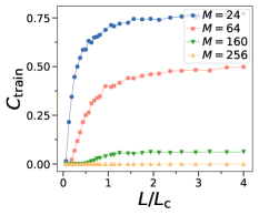
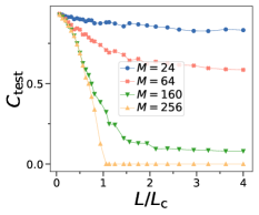
 a  b  c

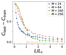
Figure 6: Training error, test error and empirical risk for hardware-efficient ansatz with haar random training states for $N=4$ qubits. We assume that there is an optimal solution, i.e. there is at least one parameter with $C_{\text{test}}(\boldsymbol{\theta_{\text{g}}})=0$. a) $C_{\text{train}}$ against $L$ for different $M$. b) $C_{\text{test}}$ against $L$ for different $M$. c) Empirical risk $C_{\text{test}}$-$C_{\text{test}}$ against $L$ for different $M$.

In Fig. 7 we study generalization and empirical risk for $U_{XY}$ ansatz and symmetric data $W_{p=1}$. In Fig. 7a,b we see that $C_{\text{train}}$ and $C_{\text{test}}$ decreases with $M$, and reaches near-zero for $M\geq M_{\text{c}}$. In Fig. 7c we plot the empirical risk $C_{\text{test}}-C_{\text{train}}$ against $M$. We find that the empirical risk first increases, then decreases with $M$. We also note that the empirical risk increases with $N$.

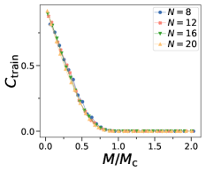
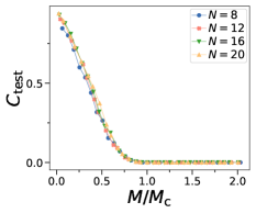
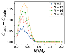
 a  b  c

Figure 7: Learning with $U_{XY}$ and $|\psi_{\ell}\rangle\in W_{p=1}$ with fixed overcomplete data $L=40\gg L_{\text{c}}$ for $N=16$. a) $C_{\text{train}}$ against $M$ for different $N$, where $M_{\text{c}}=N^{2}-1=255$. b) $C_{\text{test}}$ against $M$ for different $N$. c) Empirical risk $C_{\text{test}}-C_{\text{train}}$ against $M$.

Appendix C Training of XY model

We now show additional numerical results on training with the $U_{XY}$ ansatz and symmetric data $W_{p=1}$.

In Fig. 8a, we study generalization in the overparameterized regime. We find $C_{\text{test}}\sim 1-(L/L_{\text{c}})^{2}$ independent of $N$.

In Fig. 8b we study the steps $E$ needed to converge against $M$ for different $N$ for overcomplete data $L\gg L_{\text{c}}$. We observe $E\sim N^{2}$. At $M_{\text{c}}$ the steps needed to converge sharply decreases, indicating the transition to an optimization landscape where the global minimum can be reached easily.

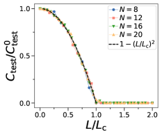
 a  b

Figure 8: Learning with $U_{XY}$ and $|\psi_{\ell}\rangle\in W_{p=1}$. a) Test error $C_{\text{test}}$ relative to error without training $C_{\text{test}}^{0}$ for varying training set size $L$ and $M\gg M_{\text{c}}$. We find $C_{\text{test}}/C_{\text{test}}^{0}=1-(L/L_{\text{c}})^{2}$, where $L_{\text{c}}=N$ and we average over 10 random instances. b) Training steps $E$ required to find $C_{\text{test}}<10^{-3}$.

Fig. 9, we show two-dimensional plots of $C_{\text{train}}$, $C_{\text{test}}$ and number of iterations $E$ against $L$ and $M$. We find training and test error matches closely the transitions derived from $R_{L}$ which are shown as black dashed lines.

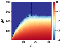
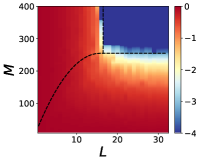
 a  b  c

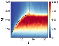
Figure 9: Mean error for training $U_{XY}$ for symmetric data $W_{p=1}$ for $N=16$ qubits. a) $C_{\text{train}}$ against $M$ and $L$. Color shows logarithm $\log_{10}(C_{\text{train}})$. b) $C_{\text{test}}$ against $M$ and $L$. c) Number of training steps $E$ until reaching $C_{\text{train}}<10^{-3}$.

Next, we show the $U_{XY}$ ansatz where we learn with random product states $W_{\text{prod}}$ in Fig.10. Here, we generalize already for $L\geq 2$. In Fig.10d, we show out-of-distribution generalization, where we train with $W_{\text{prod}}$, but test with $W_{p=1}$. We find the same test error as when testing with $W_{\text{prod}}$.

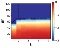
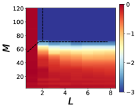
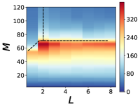
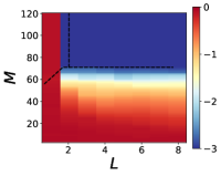
 a  b  c  d

Figure 10: Mean error for training $U_{XY}$ ansatz for random product state data sampled from $W_{\text{prod}}$ and $N=6$ qubits. a) $C_{\text{train}}$ against $M$ and $L$. Color shows logarithm $\log_{10}(C_{\text{train}})$. b) $C_{\text{test}}$ against $M$ and $L$ tested against $W_{\text{prod}}$. c) Number of training steps $E$ until reaching $C_{\text{train}}<10^{-3}$. d) Out-of-distribution generalization $C_{\text{test}}$ against $M$ and $L$ tested against $W_{p=1}$.

Appendix D Quantum Fisher information metric

The Quantum Fisher information metric (QFIM)  [57, 64] is an essential tool for quantum sensing, parameter estimation and optimization of quantum circuits. Here, we review the derivation of the QFIM or Fubini-Study metric $\mathcal{F}$ [77]. We have a parameterized quantum state $|\psi(\boldsymbol{\theta})\rangle$. We now study the variation

$$\text{d}s^{2}=|||\psi(\boldsymbol{\theta}+\text{d}\boldsymbol{\theta})\rangle-|\psi(\boldsymbol{\theta})\rangle||=\langle\delta\psi|\delta\psi\rangle=$$

$$\langle\partial_{n}\psi|\partial_{m}\psi\rangle\text{d}\boldsymbol{\theta}^{n}\boldsymbol{\theta}^{m}=(\gamma_{nm}+i\sigma_{nm})\text{d}\boldsymbol{\theta}^{n}\text{d}\boldsymbol{\theta}^{m}$$

where we defined the real and imaginary part $\gamma_{nm}$ and $\sigma_{nm}$ of $\langle\partial_{n}\psi|\partial_{m}\psi\rangle$. As $\text{d}s^{2}$ is hermitian, we have $\gamma_{nm}=\gamma_{mn}$ and $\sigma_{nm}=-\sigma_{mn}$, such that $\sigma_{nm}\text{d}\boldsymbol{\theta}^{n}\text{d}\boldsymbol{\theta}^{m}$ vanishes. However, $\gamma_{nm}$ is not a proper metric as it is not invariant under the gauge transformation $|\psi^{\prime}\rangle=\exp(i\alpha)|\psi\rangle$ under a global phase rotation with $\alpha$. We now construct a proper gauge invariant metric.

First, one can easily show by using $\langle\psi|\psi\rangle=1$ that $\beta_{n}=i\langle\psi|\partial_{n}\psi\rangle\in\mathbb{R}$. Next, we compute $\langle\psi^{\prime}|\psi^{\prime}\rangle=\gamma_{nm}^{\prime}+i\sigma_{nm}^{\prime}$, where a straightforward calculation yields

$$\gamma_{nm}^{\prime}=\gamma_{nm}+\partial_{n}\alpha\partial_{m}\alpha-\beta_{m}\gamma_{n}\alpha-\beta_{n}\gamma_{m}$$ (14)

and $\sigma_{nm}^{\prime}=\sigma_{nm}$. From this result, we now define a gauge-invariant metric

$$g_{nm}=\gamma_{nm}-\beta_{n}\beta_{m}$$ (15)

where one can easily confirm $g_{nm}^{\prime}=g_{nm}$ by using $\beta_{n}^{\prime}=\beta_{n}-\partial_{n}\alpha$. We can think of $\gamma_{nm}$ measuring the change of $|\psi(\boldsymbol{\theta})\rangle$ in the Hilbertspace, while $g_{nm}$ measures its change excluding global phases which have no observable effect.

The quantum geometric tensor is defined as

$$\Xi_{nm}=\langle\partial_{n}\psi|\partial_{m}\psi\rangle-\langle\partial_{n}\psi|\psi\rangle\langle\psi|\partial_{m}\psi\rangle$$ (16)

and the QFIM as $\mathcal{F}_{nm}=\text{Re}(\Xi_{nm})$, which corresponds to the real part of $g_{nm}$.

The QFIM describes the change in fidelity for $|\langle\psi(\boldsymbol{\theta})|\psi(\boldsymbol{\theta}+\text{d}\boldsymbol{\theta})\rangle|^{2}$ as we will see in the following. First, note that $\langle\psi|\partial_{n}\psi\rangle\in\text{Im}$. Thus, its derivative must be also imaginary, i.e. $\langle\psi|\partial_{n}\partial_{m}\psi\rangle+\langle\partial_{m}\psi|\partial_{n}\psi\rangle\in\text{Im}$, which immediately implies

$$\langle\psi|\partial_{n}\partial_{m}\psi\rangle=-\langle\partial_{m}\psi|\partial_{n}\psi\rangle\,.$$ (17)

Now, we find via Taylor expansion

$$\langle\psi(\boldsymbol{\theta})|\psi(\boldsymbol{\theta}+\text{d}\boldsymbol{\theta})\rangle\approx$$ (18)

$$1+i\langle\psi|\partial_{n}\psi\rangle\text{d}\boldsymbol{\theta}^{n}+\frac{1}{2}\langle\psi|\partial_{n}\partial_{m}\psi\rangle\text{d}\boldsymbol{\theta}^{n}\text{d}\boldsymbol{\theta}^{m}=$$

$$1+i\langle\psi|\partial_{n}\psi\rangle\text{d}\boldsymbol{\theta}^{n}-\frac{1}{2}\langle\partial_{n}\psi|\partial_{m}\psi\rangle\text{d}\boldsymbol{\theta}^{n}\text{d}\boldsymbol{\theta}^{m}$$

Now, we compute using Eq. (18)

$$|\langle\psi(\boldsymbol{\theta})|\psi(\boldsymbol{\theta}+\text{d}\boldsymbol{\theta})\rangle|^{2}=$$

$$\langle\psi(\boldsymbol{\theta})|\psi(\boldsymbol{\theta}+\text{d}\boldsymbol{\theta})\rangle\langle\psi(\boldsymbol{\theta}+\text{d}\boldsymbol{\theta})|\psi(\boldsymbol{\theta})\rangle\approx$$

$$1-[\langle\partial_{n}\psi|\psi\rangle\langle\psi|\partial_{m}\psi\rangle$$

$$+\frac{1}{2}\langle\partial_{n}\psi|\partial_{m}\psi\rangle+\frac{1}{2}\langle\partial_{m}\psi|\partial_{n}\psi\rangle]\text{d}\boldsymbol{\theta}^{n}\text{d}\boldsymbol{\theta}^{m}=$$

$$1-\text{Re}[\langle\partial_{n}\psi|\partial_{m}\psi\rangle-\langle\partial_{n}\psi|\psi\rangle\langle\psi|\partial_{m}\psi\rangle]\text{d}\boldsymbol{\theta}^{n}\text{d}\boldsymbol{\theta}^{m}.$$

where in the second step we used Eq. (17). Finally, we have

$$|\langle\psi(\boldsymbol{\theta})|\psi(\boldsymbol{\theta}+\text{d}\boldsymbol{\theta})\rangle|^{2}=1-\frac{1}{4}\mathcal{F}_{nm}\text{d}\boldsymbol{\theta}^{n}\text{d}\boldsymbol{\theta}^{m}\,.$$ (19)

This implies that $\mathcal{F}$ is a metric that describes the change in state space under a variation in parameter $\boldsymbol{\theta}$.

Appendix E Data quantum Fisher information metric

We now generalize the QFIM to the DQFIM, which describes learning $U$ with training states. We have a training set $S_{L}=\{|\psi_{\ell}\rangle,V|\psi_{\ell}\rangle\}_{\ell=1}^{L}$ and an ansatz $U(\theta)$. We learn using the cost function $C=1-L^{-1}\sum_{\ell=1}^{L}|\langle\psi_{\ell}|V^{\dagger}U(\theta)|\psi_{\ell}\rangle|^{2}$. Let us recall the projector onto the training data projector $\Pi_{L}=\sum_{k=1}^{B_{L}}|\phi_{k}\rangle\langle\phi_{k}|$ and its normalization $\tilde{\Pi}_{L}=\Pi_{L}/B_{L}$ where $|\phi_{k}\rangle$ are the eigenvectors with non-zero eigenvalue of $\rho_{L}=L^{-1}\sum_{\ell=1}^{L}|\psi_{\ell}\rangle\langle\psi_{\ell}|$ and $B_{L}=\mathrm{rank}(\rho_{L})$.

We now derive the DQFIM Eq. (23) from a variational principle in a similar manner as the QFIM. The variation of isometry $U(\theta)\Pi_{L}/\beta$ with normalization factor $\beta=\sqrt{\text{tr}(\Pi_{L})}$ is given by

$$\text{d}s^{2}=||(U(\boldsymbol{\theta}+\text{d}\boldsymbol{\theta})-U(\boldsymbol{\theta}))\Pi_{L}/\beta||=\text{tr}(\delta U^{\dagger}\tilde{\Pi}_{L}\delta U)=$$

$$\text{tr}(\partial_{n}U^{\dagger}\tilde{\Pi}_{L}\partial_{m}U)\text{d}\boldsymbol{\theta}^{n}\boldsymbol{\theta}^{m}=(\gamma_{nm}+i\sigma_{nm})\text{d}\boldsymbol{\theta}^{n}\text{d}\boldsymbol{\theta}^{m}\,,$$

where we have the difference $\delta U=U(\boldsymbol{\theta}+\text{d}\boldsymbol{\theta})-U(\boldsymbol{\theta})$, the square of the Frobenius norm $||A||=\text{tr}(A^{\dagger}A)$, the real and imaginary part $\gamma_{nm}$ and $\sigma_{nm}$ of $\text{tr}(\partial_{n}U^{\dagger}\tilde{\Pi}_{L}\partial_{m}U)$, and $\tilde{\Pi}_{L}=\Pi_{L}/\text{tr}(\Pi_{L})$. Note that we have $\text{tr}(U^{\dagger}\tilde{\Pi}_{L}U)=1$. One can now immediately check that one recovers the regular QFIM for $\rho_{1}=|\psi\rangle\langle\psi|$. As $\text{d}s^{2}$ is hermitian, we have $\gamma_{nm}=\gamma_{mn}$ and $\sigma_{nm}=-\sigma_{mn}$, such that $\sigma_{nm}\text{d}\boldsymbol{\theta}^{n}\text{d}\boldsymbol{\theta}^{m}$ vanishes. However, $\gamma_{nm}$ is not a proper metric as it is not invariant under the gauge transformation $U^{\prime}=\exp(i\alpha)U$, i.e. a global phase rotation with $\alpha$. We now construct a proper gauge invariant metric.

First, we apply $\partial_{n}$ to $\text{tr}(U^{\dagger}\tilde{\Pi}_{L}U)=1$ and see that $\text{tr}(\partial_{n}U^{\dagger}\tilde{\Pi}_{L}U)+\text{tr}(U^{\dagger}\tilde{\Pi}_{L}\partial_{n}U)=0$. It follows that $\text{tr}(U^{\dagger}\tilde{\Pi}_{L}\partial_{n}U)+\text{tr}(U^{\dagger}\tilde{\Pi}_{L}\partial_{n}U)^{\dagger}=0$ and thus $\beta_{n}=i\text{tr}(U^{\dagger}\tilde{\Pi}_{L}\partial_{n}U)\in\mathbb{R}$. Next, we compute $\text{tr}({U^{\prime}}^{\dagger}\tilde{\Pi}_{L}U^{\prime})=\gamma_{nm}^{\prime}+i\sigma_{nm}^{\prime}$, where a straightforward calculation yields

$$\gamma_{nm}^{\prime}=\gamma_{nm}+\partial_{n}\alpha\partial_{m}\alpha-\beta_{m}\gamma_{n}\alpha-\beta_{n}\gamma_{m}$$ (20)

and $\sigma_{nm}^{\prime}=\sigma_{nm}$. From this result, we now define a gauge-invariant metric

$$g_{nm}=\gamma_{nm}-\beta_{n}\beta_{m}$$ (21)

where one can easily confirm $g_{nm}^{\prime}=g_{nm}$ by using $\beta_{n}^{\prime}=\beta_{n}-\partial_{n}\alpha$. We can think of $\gamma_{nm}$ measuring the change of $U(\boldsymbol{\theta})$ in the full Hilbertspace, while $g_{nm}$ measures the change excluding global phases which have no observable effect.

In analogy to the quantum geometric tensor, we define the data quantum geometric tensor

$$\Xi_{nm}=\text{tr}(\partial_{n}U^{\dagger}\tilde{\Pi}_{L}\partial_{m}U)-\text{tr}(\partial_{n}U^{\dagger}\tilde{\Pi}_{L}U)\text{tr}(U^{\dagger}\tilde{\Pi}_{L}\partial_{m}U)$$ (22)

and the DQFIM as $\mathcal{Q}_{nm}=\text{Re}(\Xi_{nm})$, which corresponds to the real part of $g_{nm}$, with

$$\mathcal{Q}_{nm}(S_{L},U(\boldsymbol{\theta}))=4\text{Re}(\text{tr}(\partial_{n}U^{\dagger}\tilde{\Pi}_{L}\partial_{m}U)-\text{tr}(\partial_{n}U^{\dagger}\tilde{\Pi}_{L}U)\text{tr}(U^{\dagger}\tilde{\Pi}_{L}\partial_{m}U))\,.$$ (23)

Indeed, we find for $L=1$ that $\mathcal{Q}(S_{1})=\mathcal{F}$. In contrast, for a training set with $\Pi_{L}=I$, we find what we call the unitary QFIM

$$\mathcal{Q}_{nm}^{I}=4\text{Re}(d^{-1}\text{tr}(\partial_{n}U^{\dagger}\partial_{m}U)-d^{-2}\text{tr}(\partial_{n}U^{\dagger}U)\text{tr}(U^{\dagger}\partial_{m}U))\,.$$ (24)

The DQFIM describes the change of $|\text{tr}(U(\boldsymbol{\theta})^{\dagger}\tilde{\Pi}_{L}U(\boldsymbol{\theta}+\text{d}\boldsymbol{\theta}))|^{2}$ which we are going to show in the following. First, note that $\text{tr}(U^{\dagger}\tilde{\Pi}_{L}\partial_{n}U)\in\text{Im}$. Thus, its derivative must be also imaginary, i.e. $\text{tr}(U^{\dagger}\tilde{\Pi}_{L}\partial_{n}\partial_{m}U)+\text{tr}(\partial_{n}U^{\dagger}\tilde{\Pi}_{L}\partial_{m}U)\in\text{Im}$, which immediately implies

$$\text{tr}(U^{\dagger}\tilde{\Pi}_{L}\partial_{n}\partial_{m}U)=-\text{tr}(\partial_{n}U^{\dagger}\tilde{\Pi}_{L}\partial_{m}U)\,.$$ (25)

Now, we find via Taylor expansion

$$\text{tr}(U(\boldsymbol{\theta})^{\dagger}\rho_{L}U(\boldsymbol{\theta}+\text{d}\boldsymbol{\theta}))\approx$$ (26)

$$1+i\text{tr}(U^{\dagger}\tilde{\Pi}_{L}\partial_{n}U)\text{d}\boldsymbol{\theta}^{n}+\frac{1}{2}\text{tr}(U^{\dagger}\tilde{\Pi}_{L}\partial_{n}\partial_{m}U)\text{d}\boldsymbol{\theta}^{n}\text{d}\boldsymbol{\theta}^{m}=$$

$$1+i\text{tr}(U^{\dagger}\tilde{\Pi}_{L}\partial_{n}U)\text{d}\boldsymbol{\theta}^{n}-\frac{1}{2}\text{tr}(\partial_{n}U^{\dagger}\tilde{\Pi}_{L}\partial_{m}U)\text{d}\boldsymbol{\theta}^{n}\text{d}\boldsymbol{\theta}^{m}$$

Now, we compute using Eq. (26)

$$|\text{tr}(U(\boldsymbol{\theta})^{\dagger}\tilde{\Pi}_{L}U(\boldsymbol{\theta}+\text{d}\boldsymbol{\theta}))|^{2}=$$

$$\text{tr}(U(\boldsymbol{\theta})^{\dagger}\tilde{\Pi}_{L}U(\boldsymbol{\theta}+\text{d}\boldsymbol{\theta}))\text{tr}(U(\boldsymbol{\theta}+\text{d}\boldsymbol{\theta})^{\dagger}U(\boldsymbol{\theta}))\approx$$

$$1-[\text{tr}(\partial_{n}U^{\dagger}\tilde{\Pi}_{L}U)\text{tr}(U^{\dagger}\tilde{\Pi}_{L}\partial_{m}U)$$

$$+\frac{1}{2}\text{tr}(\partial_{n}U^{\dagger}\tilde{\Pi}_{L}\partial_{m}U)+\frac{1}{2}\text{tr}(\partial_{m}U^{\dagger}\tilde{\Pi}_{L}\partial_{n}U)]\text{d}\boldsymbol{\theta}^{n}\text{d}\boldsymbol{\theta}^{m}=$$

$$1-\text{Re}[\text{tr}(\partial_{n}U^{\dagger}\tilde{\Pi}_{L}\partial_{m}U)-$$

$$\text{tr}(\partial_{n}U^{\dagger}\tilde{\Pi}_{L}U)\text{tr}(U^{\dagger}\partial_{m}\tilde{\Pi}_{L}U)]\text{d}\boldsymbol{\theta}^{n}\text{d}\boldsymbol{\theta}^{m}.$$

where in the second step we used Eq. (25). Finally, we have

$$|\text{tr}(U(\boldsymbol{\theta})^{\dagger}\tilde{\Pi}_{L}U(\boldsymbol{\theta}+\text{d}\boldsymbol{\theta}))|^{2}=1-\frac{1}{4}\mathcal{Q}_{nm}\text{d}\boldsymbol{\theta}^{n}\text{d}\boldsymbol{\theta}^{m}\,,$$ (27)

which relates a change in parameter $\boldsymbol{\theta}$ to the change in the unitary projected onto the training states.

Appendix F Degrees of freedom of isometries

Now, we calculate the degrees of freedom when learning a training set of $L$ states with a $d$-dimensional unitary

$$U=\sum_{n,k=1}^{d}u_{nk}|n\rangle\langle k|$$ (28)

with $u_{nk}=a_{nk}+ib_{nk}$, where $a_{nk}$, $b_{nk}$ are real parameters. First, note that $U$ can be described using $2d^{2}$ real parameters, however due to $U^{\dagger}U=I$ and global phase, only $d^{2}-1$ real parameters are independent. We now compute the maximal number of degrees of freedom when $U$ is projected onto a training set of $L$ states. For any set $S_{L}$ of training states, the rank of the projector $\Pi_{L}$ is upper bounded by $\text{rank}(\Pi_{L})\leq L$.

We apply $U$ Eq. (28) on a training set $\{|\ell\rangle\}_{\ell=1}^{L}$ of $L$ states, where $|\ell\rangle$ are computational basis states. For a single training state $L=1$, we have $U|1\rangle=\sum_{n=1}^{d}u_{n1}|n\rangle$. Via training, we can only learn the column vector $u_{1}=(u_{11},u_{21},\dots,u_{d1})$, which has $2d$ real parameters and $2d-2$ independent parameters due to constraints of global phase and norm $\sum_{n=1}^{d}|u_{n1}|^{2}=1$. However, all other column vectors besides $u_{1}$ cannot be learned. With the DQFIM we find $R_{1}=2d-2$, i.e. $R_{1}$ indeed counts the number of degrees of freedom that can be learned. Next, we consider $L=2$. Here, we additional have the state $U|2\rangle=\sum_{n=1}^{d}u_{n2}|n\rangle$ and we can also learn the vector $u_{2}=(u_{12},u_{22},\dots,u_{d2})$ with $2d$ real parameters. However, due to unitarity, $u_{2}$ must be orthogonal to $u_{1}$, which removes two degrees of freedom. Additionally, we have to subtract one parameter for the norm condition. The global phase has already been incorporated in $u_{1}$, thus $u_{2}$ holds $2d-3$ degrees of freedom, with the $d\times 2$-dimensional isometry $(u_{1},u_{2})$ combined having $R_{2}=4d-5$. For any $L$, each additional training state adds a column $u_{L}$, which has additional $2d-2L+1$ degrees of freedom due to $L-1$ orthogonality conditions [69]. For $L$ states, we have the isometry $U_{L}=(u_{1},\dots,u_{L})$, which can be described using

$$R_{L}=(2d-2)L-(L-1)^{2}=2dL-L^{2}-1$$ (29)

real independent parameters and for $L\geq 1$. The maximum is reached for $L_{\text{c}}=d$ with $R_{d}=d^{2}-1$ and $U\Pi_{d}=U$ with $\Pi_{d}=I$, where we can completely learn $U$. For further increase in $L$ we find that $R_{L}$ stays constant. As our choice of $U$ is a generic representation of a unitary and our chosen training set has maximal rank $\text{rank}(\Pi_{L})=L$, our calculation gives us the upper bound for $R_{L}$. Note that by choosing a more constrained ansatz unitary and training sets $R_{L}$ can be smaller.

For an arbitrary unitary, the gain in effective dimension by increasing dataset size $L\rightarrow L+1$ is given by $\Delta R_{L}=R_{L+1}-R_{L}=\text{max}(2d-2L-1,0)$ for $L\geq 1$, and $\Delta R_{0}=2d-2$ for $L=0$. Thus, the gain decreases with $L$, i.e. with increasing $L$ each additional state reveals less degrees of information of $U$.

Appendix G Lie-algebra bounds DQFIM

Recall that our ansatz Eq. (12) consist of $G$ layers with

$$U(\boldsymbol{\theta})=\prod_{k=1}^{G}U_{k}(\boldsymbol{\theta}_{k})\,\,\text{with}\,\,U^{(k)}(\theta_{k})=\prod_{n=1}^{K}\exp(-i\theta_{kn}H_{n})$$ (30)

where $U^{(k)}(\theta_{k})$ is the unitary of the $k$th layer. Here, $H_{n}$ are $K$ hermitian matrices and $\boldsymbol{\theta}_{k}=\{\theta_{k1},\dots,\theta_{kn}\}$ are the parameters of the $k$th layer. The total parameter vector $\theta=\{\boldsymbol{\theta}_{1},\dots,\boldsymbol{\theta}_{G}\}$ of the ansatz has $M=GK$ parameters.

To simplify the notation, we treat each parameter entry as its own layer and relabel each generators $H_{k}$ such that we can write the ansatz as

$$U(\boldsymbol{\theta})=\prod_{k=1}^{M}\exp(-i\theta_{k}H_{k})\,.$$ (31)

First, we define the generators of the ansatz $U$ [78, 37]:

Definition 5 (Set of generators $\mathcal{T}$).

Consider ansatz Eq. (31). The set of generators $\mathcal{T}=\{H_{k}\}_{k=1}^{K}$ (with size $|\mathcal{T}|=K$) are defined as the set of Hermitian operators that generate the unitaries of each layer of $U(\boldsymbol{\theta})$.

Further the dynamical Lie Algebra $\mathfrak{g}$ is given by:

Definition 6 (Dynamical Lie Algebra (DLA)).

Consider the generators $\mathcal{T}$ according to Def. 5. The DLA $\mathfrak{g}$ is generated by repeated nested commutators of the operators in $\mathcal{T}$

$$\mathfrak{g}=\mathrm{span}\left\langle iH_{1},\ldots,iH_{K}\right\rangle_{\text{Lie}}\,,$$ (32)

where $\left\langle\mathcal{S}\right\rangle_{\text{Lie}}$ is the Lie closure, which is the set obtained by repeatedly taking the commutator of the elements in $\mathcal{S}$.

Next, we show that the DLA bounds the rank of the DQFIM. First, lets recall the entries of the matrix of the DQFIM

$$\mathcal{Q}_{nm}(S_{L},U(\boldsymbol{\theta}))=4\text{Re}(\text{tr}(\partial_{n}U^{\dagger}\tilde{\Pi}_{L}\partial_{m}U)-\text{tr}(\partial_{n}U^{\dagger}\tilde{\Pi}_{L}U)\text{tr}(U^{\dagger}\tilde{\Pi}_{L}\partial_{m}U))\,.$$ (33)

where we shorten $U=U(\boldsymbol{\theta})$, $\tilde{\Pi}_{L}=\Pi_{L}/\text{rank}(\Pi_{L})$ is the normalized projector onto the space spanned by the training states and $\partial_{n}U$ the derivative in respect to the $n$th element of parameter vector $\boldsymbol{\theta}$.

We now restate Theorem 1 for convenience.

Theorem 2.

The maximal rank $R_{L}$ of the DQFIM is upper bounded by the dimension of the dynamical Lie algebra (DLA) $\dim(\mathfrak{g})$

$$R_{L}\leq\dim(\mathfrak{g})\,,$$ (34)

where $\mathfrak{g}=\mathrm{span}\left\langle iH_{1},\ldots,iH_{K}\right\rangle_{\text{Lie}}$ is generated by the repeated nested commutators of the generators $H_{k}$ of the unitary $U(\boldsymbol{\theta})$.

The proof follows in analogy to the bound of the QFIM (i.e. $R_{1}$) of Ref. [37].

First, we note that $R_{L}\leq R_{\infty}$ as $L$ simply increases the dimension of the projector $\Pi_{L}$. Now, we assume $S_{L}$ spans the complete relevant Hilbertspace with $\Pi_{L}=I$ and thus we can simplify to the unitary QFIM

$$\mathcal{Q}_{nm}=4\text{Re}(d^{-1}\text{tr}(\partial_{n}U^{\dagger}\partial_{m}U)-d^{-2}\text{tr}(\partial_{n}U^{\dagger}U)\text{tr}(U^{\dagger}\partial_{m}U))\,.$$ (35)

As we have $\partial_{n}\exp(-i\theta_{n}H_{n})=-iH_{n}\exp(-i\theta_{n}H_{n})$, we can write the derivatives as

$$\partial_{n}U(\boldsymbol{\theta})=-iU_{n+1\rightarrow M}H_{n}U_{1\rightarrow n}\,.$$ (36)

Here, we define

$$U_{m\rightarrow n}=U_{n}U_{n-1}\dots U_{m+1}U_{m}$$ (37)

as the propagator from layer $m$ to layer $n$ and

$$\tilde{H}_{k}=U_{1\rightarrow k}^{\dagger}H_{k}U_{1\rightarrow k}\,.$$ (38)

Using above expressions, we find for the first term of the DQFIM Eq. (33)

$$\text{Re}(\text{tr}(\partial_{n}U^{\dagger}\partial_{m}U)=\text{Re}(i(-i)\text{tr}(U_{1\rightarrow n}^{\dagger}H_{n}U_{n+1\rightarrow M}^{\dagger}U_{m+1\rightarrow M}H_{m}U_{1\rightarrow m}))=\text{Re}(\text{tr}(\tilde{H}_{n}\tilde{H}_{m}))\,.$$

Similarly, we find for the second term of Eq. (33)

$$\text{Re}(\text{tr}(\partial_{n}U^{\dagger}U)\text{tr}(U^{\dagger}\tilde{\Pi}_{L}\partial_{m}U))=\text{Re}(i(-i)\text{tr}(U_{1\rightarrow n}^{\dagger}H_{n}U_{n+1\rightarrow M}^{\dagger}U_{1\rightarrow M})\cdot$$

$$\text{tr}(U_{1\rightarrow M}^{\dagger}U_{m+1\rightarrow M}H_{m}U_{1\rightarrow m}))=\text{Re}(\text{tr}(\tilde{H}_{n})\text{tr}(\tilde{H}_{m}))\,.$$

We combine these results to get the DQFIM as

$$\begin{split}\mathcal{Q}_{mn}^{I}=\text{Re}(d^{-1}\text{tr}(\tilde{H}_{n}\tilde{H}_{m})-d^{-2}\text{tr}(\tilde{H}_{n})\text{tr}(\tilde{H}_{m}))\end{split}$$ (39)

Note that $H_{k}$ are elements of the DLA $\mathfrak{g}$. As the unitaries $U_{n}$ of the ansatz are also elements of the dynamical Lie group generated by $\mathfrak{g}$, a product of $H_{k}$ with any $U_{n}$ will yield another element of the dynamical Lie group. Thus, we can always expand $\tilde{H}_{k}$ using the DLA as a basis with $\text{dim}(\mathfrak{g})$ elements:

$$\tilde{H_{k}}=\sum_{m=1}^{\text{dim}(\mathfrak{g})}a_{m}^{(k)}\chi_{m}\,,$$ (40)

where $a_{m}^{(k)}$ are real coefficients and $\{\chi_{m}\}_{m=1}^{\text{dim}(\mathfrak{g})}$ are a basis of the DLA $\mathfrak{g}$. Thus, the matrix of the DQFIM $\mathcal{Q}$ can be expressed in a basis with $\text{dim}(\mathfrak{g})$ elements. Thus, the rank of $\mathcal{Q}$ is upper bounded by the dimension of the DLA $\mathfrak{g}$

$$R_{L}\leq\text{rank}(\mathcal{Q}^{I})\leq\text{dim}(\mathfrak{g})\,.$$ (41)

Appendix H Ansatz unitaries for SM

Next, in Fig.11 we show additional ansatz unitaries which are considered in the next sections of the SM.

 

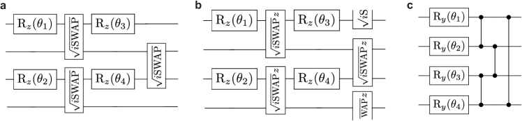
Figure 11: Ansatz unitaries for the the supplemental materials. The circuits are repeated for $G$ layers. a) $U_{XY}^{\text{open}}$ circuit with open boundary condition, i.e. the $\sqrt{\text{iSWAP}}$ do not cross from the first to the last qubit in contrast to $U_{XY}$. Commutes with particle number operator $P$ and for sufficient depth can realize any time evolution generated by $\exp(-iH_{XY}^{\text{open}}t)$. b) $U_{XXZ}$ circuit related to evolution of Heisenberg model $H_{XXZ}$. Composed of parameterized single qubit $z$ rotations and the $\sqrt{\text{iSWAP}}z$ gate defined in the text. c) Real-valued ansatz $U_{\text{Y-CZ}}$ consisting of $y$-rotations and control-$Z$ gates in a nearest-neighbor chain configuration.

In Fig.11a we show the $U_{XY}^{\text{open}}$ circuit, which is the same as the $U_{XY}$ circuit but with open boundary conditions, i.e. the $\sqrt{\text{iSWAP}}$ gates that interact between the first and last qubit are removed. This ansatz conserves particle number $P$.

In Fig.11b we show the $U_{XXZ}$ ansatz, which is composed of parameterized $z$ rotations and the $\sqrt{\text{iSWAP}}z=\sqrt{\text{CZ}}\sqrt{\text{iSWAP}}$ gate, where $\sqrt{\text{CZ}}=\text{diag}(1,1,1,i)$ is the square-root of the control-$Z$ gate. This ansatz conserves particle number $P$.

In Fig.11c we show the $U_{Y-CZ}$ ansatz [48], consisting of parameterized $y$-rotations and control-$Z$ gate $\text{diag}(1,1,1,-1)$. Due to its connection to Cluster-state generation, it overparameterizes with a polynomial number of parameters with $R_{L}\propto N^{2}$.

Appendix I Generalization with further models

Here, we study the number of training states needed for generalization for further models.

First, in Fig.12a we study the $U_{XY}^{\text{open}}$ ansatz shown in Fig.11a. This ansatz describes the evolution of the $H_{XY}^{\text{open}}=\sum_{k=1}^{N}h_{k}\sigma_{k}^{z}+\sum_{k=1}^{N-1}(\sigma_{k}^{x}\sigma_{k+1}^{x}+\sigma_{k}^{y}\sigma_{k+1}^{y})$ Hamiltonian with open boundary conditions. The difference to $H_{XY}$ is the absence of interaction between first and last qubit. We find generalization for $L=1$ training states and $M\geq M_{\text{c}}$ when using random product states as training data. A similar ansatz was studied numerically in Ref. [10]. It was shown numerically that only $1$ training state was needed for generalization, and $O(N^{2})$ gates for successful training. Here, we explain this result with the DQFIM. In particular, our ansatz has the maximal rank of the DQFIM with $R_{L}=R_{1}=R_{\infty}=N^{2}$ for all $N$. This implies that $L_{\text{c}}=1$ training state is sufficient to get an overcomplete model and achieve generalization.

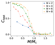
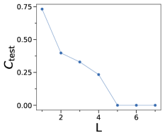
 a  b

Figure 12: a) Test error $C_{\text{test}}$ for $U_{XY}^{\text{open}}$ ansatz and for $L=1$ product training states against circuit parameters $M$. $C_{\text{test}}$ is averaged over 20 random instances. $M_{\text{c}}$ is determined with the DQFIM. b) $C_{\text{test}}$ for $U_{XZZ}$ ansatz for product training states against $L$ for $N=4$ and $M=100$.

Next, we study the $U_{XXZ}$ ansatz shown in Fig.11b. This model can describes the evolution of the $H_{XXZ}=\sum_{k=1}^{N}h_{k}\sigma_{k}^{z}+\sum_{k=1}^{N}(\sigma_{k}^{x}\sigma_{k+1}^{x}+\sigma_{k}^{y}\sigma_{k+1}^{y}+\Delta\sigma_{k}^{z}\sigma_{k+1}^{z})$ Hamiltonian. A similar ansatz was studied in Ref. [10]. It was numerically shown that $5$ training states are needed for generalization for $N=4$. In Fig.12b, we show the test error of the $U_{XXZ}$ ansatz against $L$ in the overparameterized regime and indeed find the test error vanishes for $L\geq 5$. Using the DQFIM, we find $R_{1}=24$ and $R_{\infty}=R_{L_{\text{c}}}=51$ with $L_{\text{c}}=5$, matching the numerical results. Thus, the DQFIM accurately predicts the needed training states. Note that the approximation $L_{\text{c}}\approx 2R_{\infty}/R_{1}=4.25$ gives a good estimation of the number of needed training states as well.

Appendix J Training of Y-CZ model

We show numerical results on training with the $U_{\text{Y-CZ}}$ ansatz (see Fig. 11c for definition) in Fig. 13. This model requires $L=2$ states to generalize as we have $R_{L}\sim N^{2}$. We find training and test error matches closely the transitions derived from $R_{L}$ shown as black dashed lines.

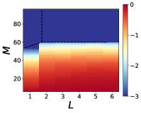
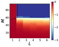
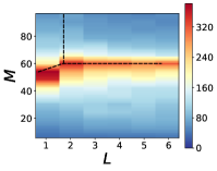
 a  b  c

Figure 13: Mean error for training $U_{\text{Y-CZ}}$ for product state as training data and $N=6$ qubits. a) $C_{\text{train}}$ against $M$ and $L$. Color shows logarithm $\log_{10}(C_{\text{train}})$. b) $C_{\text{test}}$ against $M$ and $L$. c) Number of training steps $E$ until reaching $C_{\text{train}}<10^{-3}$.

References

Biamonte et al. [2017]J. Biamonte, P. Wittek,
N. Pancotti, P. Rebentrost, N. Wiebe, and S. Lloyd, Quantum machine learning, Nature 549, 195 (2017).
Poland et al. [2020]K. Poland, K. Beer, and T. J. Osborne, No free lunch for quantum machine
learning, arXiv
preprint arXiv:2003.14103 (2020).
Caro and Datta [2020]M. C. Caro and I. Datta, Pseudo-dimension of quantum
circuits, Quantum Machine Intelligence 2, 14 (2020).
Abbas et al. [2021a]A. Abbas, D. Sutter,
C. Zoufal, A. Lucchi, A. Figalli, and S. Woerner, The power of quantum neural networks, Nature Computational Science 1, 403 (2021a).
Abbas et al. [2021b]A. Abbas, D. Sutter,
A. Figalli, and S. Woerner, Effective dimension of machine learning models, arXiv:2112.04807 (2021b).
Sharma et al. [2022]K. Sharma, M. Cerezo,
Z. Holmes, L. Cincio, A. Sornborger, and P. J. Coles, Reformulation of the no-free-lunch theorem for entangled datasets, Physical Review
Letters 128, 070501
(2022).
Banchi et al. [2021]L. Banchi, J. Pereira, and S. Pirandola, Generalization in quantum machine
learning: A quantum information standpoint, PRX Quantum 2, 040321 (2021).
Caro et al. [2022a]M. C. Caro, H.-Y. Huang,
N. Ezzell, J. Gibbs, A. T. Sornborger, L. Cincio, P. J. Coles, and Z. Holmes, Out-of-distribution generalization for learning quantum dynamics, arXiv:2204.10268 (2022a).
Peters and Schuld [2022]E. Peters and M. Schuld, Generalization despite
overfitting in quantum machine learning models, arXiv:2209.05523 (2022).
Gibbs et al. [2022a]J. Gibbs, Z. Holmes,
M. C. Caro, N. Ezzell, H.-Y. Huang, L. Cincio, A. T. Sornborger, and P. J. Coles, Dynamical simulation via quantum machine learning with provable
generalization, arXiv:2204.10269 (2022a).
Volkoff et al. [2021]T. Volkoff, Z. Holmes, and A. Sornborger, Universal compiling and (no-)
free-lunch theorems for continuous-variable quantum learning, PRX Quantum 2, 040327 (2021).
Cai et al. [2022]H. Cai, Q. Ye, and D.-L. Deng, Sample complexity of learning parametric quantum
circuits, Quantum Science and Technology 7, 025014 (2022).
Popescu [2021]C. M. Popescu, Learning bounds for
quantum circuits in the agnostic setting, Quantum Information Processing 20, 286 (2021).
Caro et al. [2021]M. C. Caro, E. Gil-Fuster,
J. J. Meyer, J. Eisert, and R. Sweke, Encoding-dependent generalization bounds for parametrized quantum
circuits, Quantum 5, 582
(2021).
Bu et al. [2022]K. Bu, D. E. Koh,
L. Li, Q. Luo, and Y. Zhang, Statistical complexity of quantum circuits, Physical Review A 105, 062431 (2022).
Bowles et al. [2023]J. Bowles, V. J. Wright,
M. Farkas, N. Killoran, and M. Schuld, Contextuality and inductive bias in quantum machine
learning, arXiv:2302.01365 (2023).
Du et al. [2022]Y. Du, Y. Yang, D. Tao, and M.-H. Hsieh, Demystify problem-dependent power of quantum neural networks on
multi-class classification, arXiv:2301.01597 (2022).
Bisio et al. [2010]A. Bisio, G. Chiribella,
G. M. D’Ariano,
S. Facchini, and P. Perinotti, Optimal quantum learning of a unitary
transformation, Physical Review A 81, 032324 (2010).
Marvian and Lloyd [2016]I. Marvian and S. Lloyd, Universal quantum
emulator, arXiv
preprint arXiv:1606.02734 (2016).
Bharti et al. [2022]K. Bharti, A. Cervera-Lierta, T. H. Kyaw, T. Haug, S. Alperin-Lea, A. Anand, M. Degroote, H. Heimonen, J. S. Kottmann, T. Menke, W.-K. Mok,
S. Sim, L.-C. Kwek, and A. Aspuru-Guzik, Noisy intermediate-scale quantum algorithms, Rev. Mod. Phys. 94, 015004 (2022).
Cerezo et al. [2021]M. Cerezo, A. Arrasmith,
R. Babbush, S. C. Benjamin, S. Endo, K. Fujii, J. R. McClean, K. Mitarai, X. Yuan,
L. Cincio, et al., Variational quantum
algorithms, Nature Reviews Physics 3, 625 (2021).
Xue et al. [2022]S. Xue, Y. Liu, Y. Wang, P. Zhu, C. Guo, and J. Wu, Variational
quantum process tomography of unitaries, Physical Review A 105, 032427 (2022).
Gebhart et al. [2023]V. Gebhart, R. Santagati,
A. A. Gentile, E. M. Gauger, D. Craig, N. Ares, L. Banchi, F. Marquardt,
L. Pezzè, and C. Bonato, Learning quantum systems, Nature Reviews Physics , 1 (2023).
Kiani et al. [2020]B. T. Kiani, S. Lloyd, and R. Maity, Learning unitaries by gradient descent, arXiv:2001.11897 (2020).
Khatri et al. [2019]S. Khatri, R. LaRose,
A. Poremba, L. Cincio, A. T. Sornborger, and P. J. Coles, Quantum-assisted quantum compiling, Quantum 3, 140 (2019).
Ezzell et al. [2022]N. Ezzell, E. M. Ball,
A. U. Siddiqui, M. M. Wilde, A. T. Sornborger, P. J. Coles, and Z. Holmes, Quantum mixed state compiling, arXiv:2209.00528 (2022).
Cirstoiu et al. [2020]C. Cirstoiu, Z. Holmes,
J. Iosue, L. Cincio, P. J. Coles, and A. Sornborger, Variational fast forwarding for quantum simulation beyond
the coherence time, npj Quantum Information 6, 82 (2020).
Gibbs et al. [2022b]J. Gibbs, K. Gili,
Z. Holmes, B. Commeau, A. Arrasmith, L. Cincio, P. J. Coles, and A. Sornborger, Long-time simulations for fixed input states on quantum hardware, npj Quantum
Information 8, 135
(2022b).
Romero et al. [2017]J. Romero, J. P. Olson, and A. Aspuru-Guzik, Quantum autoencoders for efficient
compression of quantum data, Quantum Sci. Technol. 2, 045001 (2017).
Zhang et al. [2022]H. Zhang, L. Wan, T. Haug, W.-K. Mok, S. Paesani, Y. Shi, H. Cai, L. K. Chin,
M. F. Karim, L. Xiao, et al., Resource-efficient high-dimensional
subspace teleportation with a quantum autoencoder, Science Advances 8, eabn9783 (2022).
Leone et al. [2022]L. Leone, S. F. Oliviero,
S. Piemontese, S. True, and A. Hamma, Retrieving information from a black hole using quantum machine
learning, Physical Review A 106, 062434 (2022).
Anschuetz [2021]E. R. Anschuetz, Critical points in
quantum generative models, arXiv:2109.06957 (2021).
Anschuetz and Kiani [2022]E. R. Anschuetz and B. T. Kiani, Quantum variational
algorithms are swamped with traps, Nature Communications 13, 7760 (2022).
Bittel and Kliesch [2021]L. Bittel and M. Kliesch, Training variational
quantum algorithms is np-hard, Physical review letters 127, 120502 (2021).
You and Wu [2021]X. You and X. Wu, Exponentially many local minima in
quantum neural networks, in International Conference on Machine Learning (PMLR, 2021) pp. 12144–12155.
McClean et al. [2018]J. R. McClean, S. Boixo,
V. N. Smelyanskiy,
R. Babbush, and H. Neven, Barren plateaus in quantum neural network training
landscapes, Nature communications 9, 4812 (2018).
Larocca et al. [2021]M. Larocca, N. Ju,
D. García-Martín, P. J. Coles, and M. Cerezo, Theory
of overparametrization in quantum neural networks, arXiv:2109.11676 (2021).
You et al. [2022]X. You, S. Chakrabarti, and X. Wu, A convergence theory for over-parameterized
variational quantum eigensolvers, arXiv:2205.12481 (2022).
Wiersema et al. [2020]R. Wiersema, C. Zhou,
Y. de Sereville, J. F. Carrasquilla, Y. B. Kim, and H. Yuen, Exploring entanglement and optimization within the hamiltonian
variational ansatz, PRX Quantum 1, 020319 (2020).
Schatzki et al. [2022]L. Schatzki, M. Larocca,
F. Sauvage, and M. Cerezo, Theoretical guarantees for permutation-equivariant quantum
neural networks, arXiv:2210.09974 (2022).
Ragone et al. [2022]M. Ragone, P. Braccia,
Q. T. Nguyen, L. Schatzki, P. J. Coles, F. Sauvage, M. Larocca, and M. Cerezo, Representation theory for geometric quantum machine learning, arXiv:2210.07980 (2022).
Nguyen et al. [2022]Q. T. Nguyen, L. Schatzki,
P. Braccia, M. Ragone, P. J. Coles, F. Sauvage, M. Larocca, and M. Cerezo, Theory
for equivariant quantum neural networks, arXiv:2210.08566 (2022).
Zheng et al. [2021]H. Zheng, Z. Li, J. Liu, S. Strelchuk, and R. Kondor, Speeding up learning quantum states through group equivariant
convolutional quantum ansätze, arXiv:2112.07611 (2021).
Meyer et al. [2023]J. J. Meyer, M. Mularski,
E. Gil-Fuster, A. A. Mele, F. Arzani, A. Wilms, and J. Eisert, Exploiting symmetry in variational quantum machine learning, PRX Quantum 4, 010328 (2023).
Larocca et al. [2022]M. Larocca, F. Sauvage,
F. M. Sbahi, G. Verdon, P. J. Coles, and M. Cerezo, Group-invariant quantum machine learning, PRX Quantum 3, 030341 (2022).
Sauvage et al. [2022]F. Sauvage, M. Larocca,
P. J. Coles, and M. Cerezo, Building spatial symmetries into parameterized
quantum circuits for faster training, arXiv:2207.14413 (2022).
Skolik et al. [2022]A. Skolik, M. Cattelan,
S. Yarkoni, T. Bäck, and V. Dunjko, Equivariant quantum circuits for learning on weighted
graphs, arXiv
preprint arXiv:2205.06109 (2022).
Haug et al. [2021]T. Haug, K. Bharti, and M. Kim, Capacity and quantum geometry of parametrized
quantum circuits, PRX Quantum 2, 040309 (2021).
Anschuetz et al. [2022]E. R. Anschuetz, A. Bauer,
B. T. Kiani, and S. Lloyd, Efficient classical algorithms for simulating
symmetric quantum systems, arXiv preprint arXiv:2211.16998 (2022).
Huang et al. [2021]H.-Y. Huang, M. Broughton,
M. Mohseni, R. Babbush, S. Boixo, H. Neven, and J. R. McClean, Power of
data in quantum machine learning, Nature communications 12, 1 (2021).
Liu et al. [2021]Y. Liu, S. Arunachalam, and K. Temme, A rigorous and robust quantum speed-up in
supervised machine learning, Nature Physics , 1 (2021).
Huang et al. [2022]H.-Y. Huang, R. Kueng,
G. Torlai, V. V. Albert, and J. Preskill, Provably efficient machine learning for quantum many-body
problems, Science 377, eabk3333
(2022).
Liu et al. [2023]J. Liu, M. Liu, J.-P. Liu, Z. Ye, Y. Alexeev, J. Eisert, and L. Jiang, Towards
provably efficient quantum algorithms for large-scale machine-learning
models, arXiv:2303.03428 (2023).
Bartlett et al. [2017]P. L. Bartlett, D. J. Foster, and M. J. Telgarsky, Spectrally-normalized
margin bounds for neural networks, Advances in neural information processing systems 30 (2017).
Jiang et al. [2019]Y. Jiang, B. Neyshabur,
H. Mobahi, D. Krishnan, and S. Bengio, Fantastic generalization measures and where to find
them, arXiv:1912.02178 (2019).
Liang et al. [2019]T. Liang, T. Poggio,
A. Rakhlin, and J. Stokes, Fisher-rao metric, geometry, and complexity of neural
networks, in The 22nd
international conference on artificial intelligence and statistics (PMLR, 2019) pp. 888–896.
Meyer [2021]J. J. Meyer, Fisher information in noisy
intermediate-scale quantum applications, Quantum 5, 539 (2021).
García-Martín et al. [2023]D. García-Martín, M. Larocca, and M. Cerezo, Effects
of noise on the overparametrization of quantum neural networks, arXiv:2302.05059 (2023).
Caro et al. [2022b]M. C. Caro, H.-Y. Huang,
M. Cerezo, K. Sharma, A. Sornborger, L. Cincio, and P. J. Coles, Generalization in quantum machine learning from few training data, Nature
communications 13, 4919
(2022b).
Garcia-Escartin and Chamorro-Posada [2013]J. C. Garcia-Escartin and P. Chamorro-Posada, Swap test and
hong-ou-mandel effect are equivalent, Physical Review A 87, 052330 (2013).
Chakrabarti and Rabitz [2007]R. Chakrabarti and H. Rabitz, Quantum control
landscapes, International Reviews in Physical Chemistry 26, 671 (2007).
Mitarai et al. [2018]K. Mitarai, M. Negoro,
M. Kitagawa, and K. Fujii, Quantum circuit learning, Physical Review A 98, 032309 (2018).
Nielsen and Chuang [2002]M. A. Nielsen and I. Chuang, Quantum computation and quantum
information (2002).
Liu et al. [2020]J. Liu, H. Yuan, X.-M. Lu, and X. Wang, Quantum fisher information matrix and multiparameter estimation, Journal of Physics
A: Mathematical and Theoretical 53, 023001 (2020).
Rabitz et al. [2004]H. A. Rabitz, M. M. Hsieh, and C. M. Rosenthal, Quantum optimally controlled
transition landscapes, Science 303, 1998 (2004).
Bukov et al. [2018]M. Bukov, A. G. R. Day,
D. Sels, P. Weinberg, A. Polkovnikov, and P. Mehta, Reinforcement learning in different phases of quantum control, Phys. Rev. X 8, 031086 (2018).
Johansson et al. [2012]J. R. Johansson, P. D. Nation, and F. Nori, Qutip: An open-source python framework
for the dynamics of open quantum systems, Computer Physics Communications 183, 1760 (2012).
Kökcü et al. [2022]E. Kökcü, D. Camps, L. B. Oftelie,
J. K. Freericks, W. A. de Jong, R. Van Beeumen, and A. F. Kemper, Algebraic compression of quantum circuits for hamiltonian
evolution, Physical Review A 105, 032420 (2022).
Haferkamp et al. [2022]J. Haferkamp, P. Faist,
N. B. Kothakonda,
J. Eisert, and N. Yunger Halpern, Linear growth of quantum circuit complexity, Nature Physics 18, 528 (2022).
Pérez-Salinas et al. [2020]A. Pérez-Salinas, A. Cervera-Lierta, E. Gil-Fuster, and J. I. Latorre, Data re-uploading for a
universal quantum classifier, Quantum 4, 226 (2020).
Jerbi et al. [2023]S. Jerbi, L. J. Fiderer,
H. Poulsen Nautrup,
J. M. Kübler,
H. J. Briegel, and V. Dunjko, Quantum machine learning beyond kernel methods, Nature
Communications 14, 517
(2023).
Schuld and Killoran [2019]M. Schuld and N. Killoran, Quantum machine learning
in feature hilbert spaces, Physical review letters 122, 040504 (2019).
Cheng [2010]R. Cheng, Quantum geometric tensor
(fubini-study metric) in simple quantum system: A pedagogical introduction, arXiv:1012.1337 (2010).
d’Alessandro [2021]D. d’Alessandro, Introduction to
quantum control and dynamics (Chapman and
hall/CRC, 2021).