Optimization Dynamics of Equivariant and Augmented Neural Networks

Abstract

We investigate the optimization of multilayer perceptrons on symmetric data. We compare the strategy of constraining the architecture to be equivariant to that of using augmentation. We show that, under natural assumptions on the loss and non-linearities, the sets of equivariant stationary points are identical for the two strategies, and that the set of equivariant layers is invariant under the gradient flow for augmented models. Finally, we show that stationary points may be unstable for augmented training although they are stable for the equivariant models.

1 Introduction

In machine learning, the general goal is to find ’hidden’ patterns in data. However, there are sometimes symmetries in the data that are known a priori. Incorporating these manually should, heuristically, reduce the complexity of the learning task. In this paper, we are concerned with training networks, more specifically multilayer perceptrons (MLPs) as defined below, on data exhibiting symmetries that can be formulated as equivariance under a group action. A standard example is the case of translation invariance in image classification.

More specifically, we want to theoretically study the connections between two general approaches to incorporating symmetries in MLPs. The first approach is to construct equivariant models by means of architectural design. This framework, known as Geometric Deep Learning [5, 6], exploits the geometric origin of the group $G$ of symmetry transformations by choosing the linear MLP layers and nonlinearities to be equivariant (or invariant) with respect to the action of $G$. In other words, the symmetry transformations commute with each linear (or affine) map in the network, which results in an architecture which manifestly respects the symmetry $G$ of the problem. One prominent example is the spatial weight sharing of convolutional neural networks (CNNs) which are equivariant under translations. Group equivariant convolution networks (GCNNs) [9, 28, 16] extends this principle to an exact equivariance under more general symmetry groups. The second approach is agnostic to model architecture, and instead attempts to achieve equivariance during training via data augmentation, which refers to the process of extending the training to include synthetic samples obtained by subjecting training data to random symmetry transformations.

Both approaches have their benefits and drawbacks. Equivariant models use parameters efficiently through weight sharing along the orbits of the symmetry group, but are difficult to implement and computationally expensive to evaluate in general, since they entail numerical integration over the symmetry group (see, e.g., [16]). Data augmentation, on the other hand, is agnostic to the model structure and easy to adapt to different symmetry groups. However, the augmentation strategy is by no means guaranteed to achieve a model which is exactly equivariant: the hope is that model will ’automatically’ infer invariances from the data, but there are few theoretical guarantees. Also, augmentation in general entails an inefficient use of parameters and an increase in model complexity and training required.

In this paper, we study equivariant MLPs, which can be characterized by their weights lying in a special subspace $\mathcal{E}$ of the entire parameter space $\mathcal{L}$ (both formally defined below). We use representation theory to compare and analyze the dynamics of gradient flow training of MLPs adhering to either the equivariant or augmented strategy. In particular, we study their stationary points, i.e., the potential limit points of the training, in $\mathcal{E}$. The equivariant models (of course) have optima for their gradient flow there and so are guaranteed to produce a trained model which respects the symmetry. However, the dynamics under augmented training has previously not been exhaustively explored.

Our main contributions are as follows: First, we provide a technical statement (Lemma 4) about the augmented risk: We show that it can be expressed as the nominal risk averaged over the symmetry group acting on the layers of the MLP. Using this formulation of the augmented risk, we apply standard methods from the analysis of dynamical systems to show:

1. The subspace $\mathcal{E}$ is invariant under the gradient flow of the augmented model (Corollary 1). In other words, if the augmented model is equivariantly initialized, it will remain equivariant during training.

2. The set of stationary points in $\mathcal{E}$ for the augmented model is identical to that of the equivariant model (Corollary 2). In other words, compared to the equivariant approach, augmentation introduces no new equivariant stationary points, nor does it exclude existing ones.

3. The set of strict local minima in $\mathcal{E}$ for the augmented model is a subset of the corresponding set for the equivariant model. (Proposition 3). In other words, the existence of a stable equivariant minimum is not guaranteed by augmentation.

In addition, we perform experiments on different learning tasks, with different symmetry groups, and discuss the results in the context of our theoretical developments.

2 Related work

The group theory based model for group augmentation we use here is heavily inspired by the framework developed in [7]. Augmentation and manifest invariance/equivariance have been studied from this perspective in a number of papers [20, 21, 24, 12]. More general models for data augmentation have also been considered [11]. Previous work has mostly mostly been concerned with so-called kernel and feature-averaged models (see Remark 2 below), and in particular, fully general MLPs as we treat them here have not been considered. The works have furthermore mostly been concerned with proving statistical properties of the models, and not study their dynamic at training. An exception is [21], in which it is proven that in linear scenarios, the equivariant models are optimal, but little is known about more involved models.

The dynamics of training linear equivariant networks (i.e., MLPs without nonlinearities) has been given some attention in the literature. Linear networks is a simplified, but nonetheless popular theoretical model for analysing neural networks [3]. In [18], the authors analyse the implicit bias of training a linear neural network with one fully connected layer on top of an equivariant backbone using gradient descent. They also provide some numerical results for non-linear models, but no comparison to data augmentation is made. In [8], completely equivariant linear networks are considered, and an equivalence result between augmentation and restriction is proven for binary classification tasks. However, more realistic MLPs involving non-linearities are not treated at all.

Empirical comparisons of training equivariant and augmented non-equivariant models are common in the literature. Most often, the augmented models are considered as baselines for the evaluation of the equivariant models. More systemic investigations include [14, 25, 15]. Compared to previous work, our formulation differs in that the parameter of the augmented and equivariant models are defined on the same vector spaces, which allows us to make a stringent mathematical comparison.

3 Mathematical framework

Let us begin by setting up the framework. We let $X$ and $Y$ be vector spaces and $\mathcal{D}(x,y)$ be a joint distribution on $X\times Y$. We are concerned with training an MLP $\Phi_{A}:X\to Y$ so that $y\approx\Phi_{A}(x)$. The MLP has the form

$$x_{0}=x,\quad x_{i+1}=\sigma_{i}(A_{i}x_{i}),\quad i\in[L]=\{0,\dots,L-1\},\quad\Phi_{A}(x)=x_{L},$$ (1)

where $A_{i}:X_{i}\to X_{i+1}$ are linear maps (layers) between (hidden) vector spaces $X_{i}$ with $X=X_{0}$ and $Y=X_{L}$, and $\sigma_{i}:X_{i+1}\to X_{i+1}$ are non-linearities. Note that $A=(A_{i})_{i\in[L]}$ parameterizes the network since the non-linearities are assumed to be fixed. We denote the vector space of possible linear layers with $\mathcal{L}=\bigoplus_{i\in[L]}\mathrm{Hom}(X_{i},X_{i+1})$, where $\mathrm{Hom}(X_{i},X_{i+1})$ is the space of linear maps $X_{i}\to X_{i+1}$. To train the MLP, we optimize the nominal risk

$$R(A)=\mathbb{E}_{\mathcal{D}}(\ell(\Phi_{A}(x),y)),$$ (2)

where $\ell:Y\times Y\to\mathbb{R}$ is a loss function, using gradient descent. In fact, to simplify the analysis, we will mainly study the gradient flow of the model, i.e., set the learning rate to be infinitesimal.

3.1 Representation theory and equivariance

Throughout the paper, we aim to make the MLP equivariant towards a group of symmetry transformations of the space $X\times Y$. That is, we consider a group $G$ acting on the vector spaces $X$ and $Y$ through representations $\rho_{X}$ and $\rho_{Y}$, respectively. A representation $\rho$ of a group $G$ on a vector space $V$ is a map from the group $G$ to the group of invertible linear maps $\mathrm{GL}(V)$ on $V$ that respects the group operation, i.e. $\rho(gh)=\rho(g)\rho(h)$ for all $g,h\in G$. The representation $\rho$ is unitary if $\rho(g)$ is unitary for all $g\in G$. A function $f:X\to Y$ is called equivariant with respect to $G$ if $f\circ\rho_{X}(g)=\rho_{Y}(g)\circ f$ for all $g\in G$. We denote the space of equivariant linear maps $U\to V$ by $\mathrm{Hom}_{G}(U,V)$.

Let us recall some important examples that will be used throughout the paper.

Example 1.

A simple, but important, representation is the trivial one, $\rho^{\mathrm{triv}}(g)=\mathrm{id}$ for all $g\in G$. If we equip $Y$ with the trivial representation, the equivariant functions $f:X\to Y$ are the invariant ones.

Example 2.

$\mathbb{Z}_{N}^{2}$ acts through translations on images $x\in\mathbb{R}^{N,N}$: $(\rho^{\mathrm{tr}}(k,\ell)x)_{i,j}=x_{i-k,j-\ell}$.

Further examples related to the experiments in subsequent sections are provided in Appendix B.

3.2 Training equivariant models

In order to obtain a model $\Phi_{A}$ which respects the symmetries of a group $G$ acting on $X\times Y$, we should incorporate them in our model or training strategy. Note that the distribution $\mathcal{D}(x,y)$ of training data is typically not symmetric in the sense $(x,y)\sim(\rho_{X}(g)x,\rho_{Y}(g)y)$. Instead, in the context we consider, symmetries are usually inferred from, e.g., domain knowledge of $X\times Y$. We now formally describe two strategies for training MLPs which respect equivariance under $G$.

Strategy 1: Manifest equivariance

The first method of enforcing equivariance is to constrain the layers to be manifestly equivariant. That is, we assume that $G$ is acting also on all hidden spaces $X_{i}$ through representations $\rho_{i}$, where $\rho_{0}=\rho_{X}$ and $\rho_{L}=\rho_{Y}$, and constrain each layer $L_{i}$ to be equivariant. In other words, we choose the layers $L\in\mathcal{L}$ in the equivariant subspace

$$\mathcal{E}=\bigoplus_{i\in[L]}\mathrm{Hom}_{G}(X_{i},X_{i+1})$$ (3)

If we in addition assume that all non-linearities $\sigma_{i}$ are equivariant, it is straight-forward to show that $\Phi_{A}$ is exactly equivariant under $G$ (see also Lemma 3). We will refer to these models as equivariant. The set $\mathcal{E}$ has been extensively studied in the setting of geometric deep learning and explicitly characterized in many important cases [22, 10, 16, 27, 23, 1]. In [13], a general method for determining $\mathcal{E}$ numerically directly from the $\rho_{i}$ and the structure of the group $G$ is described.

Defining $\Pi_{\mathcal{E}}:\mathcal{L}\to\mathcal{E}$ as the orthogonal projection onto $\mathcal{E}$, a convenient formulation of the strategy, which is the one we will use, is to optimize the equivariant risk

$$R^{\mathrm{eqv}}(A)=R(\Pi_{\mathcal{E}}A).$$ (4)

Strategy 2: Data augmentation

The second method we consider is to augment the training data. To this end, we define a new distribution on $X\times Y$ by drawing samples $(x,y)$ from $\mathcal{D}$ and subsequently augmenting them by applying the action of a randomly drawn group element $g\in G$ on both data $x$ and label $y$. Training on this augmented distribution can be formulated as optimizing the augmented risk

$$R^{\mathrm{aug}}(A)=\int_{G}\mathbb{E}_{\mathcal{D}}(\ell(\Phi_{A}(\rho_{X}(g)x),\rho_{Y}(g)y))\,\mathrm{d}\mu(g)$$ (5)

Here, $\mu$ is the (normalised) Haar measure on the group [17], which is defined through its invariance with respect to the action of $G$ on itself; if $h$ is distributed according to $\mu$ then so is $gh$ for all $g\in G$. This property of the Haar measure will be crucial in our analysis. Choosing another measure would cause the augmentation to be biased towards certain group elements, and is not considered here. Note that if the data $\mathcal{D}$ already is symmetric in the sense that $(x,y)\sim(\rho_{X}(g)x,\rho_{Y}(g)y)$, the augmentation acts trivially.

Remark 1.

(5) is a simplification – in practice, the actual function that is optimized is an empirical approximation of $R^{\mathrm{aug}}$ formed by sampling of the group $G$. Our results are hence about an ’infinite-augmentation limit’ that still should have high relevance at least in the ’high-augmentation region’ due to the law of large numbers. To properly analyse this transition carefully is important, but beyond the scope of this work.

In our analysis, we want to compare the two strategies when training the same model. We will make three global assumptions.

Assumption 1.

The group $G$ is acting on all hidden spaces $X_{i}$ through unitary representations $\rho_{i}$.

Assumption 2.

The non-linearities $\sigma_{i}:X_{i+1}\to X_{i+1}$ are equivariant.

Assumption 3.

The loss $\ell$ is invariant, i.e. $\ell(\rho_{Y}(g)y,\rho_{Y}(g)y^{\prime})=\ell(y,y^{\prime})$, $y,y^{\prime}\in Y$, $g\in G$.

Let us briefly comment on these assumptions. The first assumption is needed for the restriction strategy to be well defined. The technical part – the unitarity – is not a true restriction: As long as all $X_{i}$ are finite-dimensional and $G$ is compact, we can redefine the inner products on $X_{i}$ to ensure that all $\rho_{i}$ become unitary. The second assumption is required for the equivariant strategy to be sound – if the $\sigma_{i}$ are not equivariant, they will explicitly break equivariance of $\Phi_{A}$ even if $A\in\mathcal{E}$. The third assumption guarantees that the loss-landscape is ’unbiased’ towards group transformations, which is certainly required to train any model respecting the symmetry group.

We also note that all assumptions are in many settings quite weak – we already commented on Assumption 1. As for Assumption 2, note that e.g. any non-linearity acting pixel-wise on an image will be equivariant to both translations and rotations by multiples of $\pi/2$. In the same way, any loss comparing images pixel by pixel will be, so that Assumption 3 is satisfied. Furthermore, if we are trying to learn an invariant function the final representation $\rho_{Y}$ is trivial and Assumption 3 is trivially satisfied.

Remark 2.

Before proceeding, let us mention a different strategy to build equivariant models: feature averaging [20]. This strategy refers to altering the model by averaging it over the group:

$$\Phi^{\mathrm{FA}}_{A}(x):=\int_{G}\rho_{Y}(g)^{-1}\Phi_{A}(\rho_{X}(g)x)\,\mathrm{d}\mu(g).$$ (6)

In words, the value of the feature averaged network at a datapoint $x$ is obtained by calculating the outputs of the original model $\Phi_{A}$ on transformed versions of $x$, and averaging the re-adjusted outputs over $G$. Note that the modification of an MLP here does not rely on explicitly controlling the weights. It is not hard to prove (see e.g. [21, Prop. 2]) that under the invariance assumption on $\ell$,

$$R^{\mathrm{aug}}(A)=\mathbb{E}(\ell(\Phi^{\mathrm{FA}}_{A}(x),y)).$$ (7)

3.3 Lifted representations and their properties

We can lift the representations $\rho_{i}$ to representations $\overline{\rho}_{i}$ of $G$ on $\mathrm{Hom}(X_{i},X_{i+1})$ through

$$\overline{\rho}_{i}(g)A_{i}=\rho_{i+1}(g)A_{i}\rho_{i}(g)^{-1},$$ (8)

and from that derive a representation $\overline{\rho}$ on $\mathcal{L}$ according to $(\overline{\rho}(g)A)_{i}=\overline{\rho}_{i}(g)A_{i}$. Since the $\rho_{i}$ are unitary, with respect to the appropriate canonical inner products, so are $\overline{\rho}_{i}$ and $\overline{\rho}$.

Before proceeding we establish some simple, but crucial facts, concerning the lifted representation $\overline{\rho}$ and the way it appears in the general framework. We will need the following two well-known lemmas. Proofs are presented in Appendix A.

Lemma 1.

$A\in\mathcal{E}$ if and only if $\,\overline{\rho}(g)A=A$ for all $g\in G$.

Lemma 2.

For any $A\in\mathcal{L}$ the orthogonal projection $\Pi_{\mathcal{E}}$ is given by

$$\Pi_{\mathcal{E}}A=\int_{G}\overline{\rho}(g)A\,\mathrm{d}\mu(g).$$ (9)

We now prove a relation between transforming the input and transforming the layers of an MLP.

Lemma 3.

Under Assumption 2, for any $A\in\mathcal{L}$ and $g\in G$ we have

$$\Phi_{A}(\rho_{X}(g)x)=\rho_{Y}(g)\Phi_{\overline{\rho}(g)^{-1}A}(x).$$ (10)

In particular, $\Phi_{A}$ is equivariant for every $A\in\mathcal{E}$.

Proof.

The in particular part follows from $\overline{\rho}(g)^{-1}A=A$ for $A\in\mathcal{E}$. To prove the main statement, we use the notation (1): $x_{i}$ denotes the outputs of each layer of $\Phi_{A}$ when it acts on the input $x\in X$. Also, for $g\in G$, let $x_{i}^{g}$ denote the outputs of each layer of the network $\Phi_{\overline{\rho}(g)^{-1}A}$ when acting on the input $\rho_{X}(g)^{-1}x$. If we show that $\rho_{i}(g)x_{i}^{g}=x_{i}$ for $i=[L+1]$, the claim follows. We do so via induction. The case $i=0$ is clear: $\rho_{X}(g)x_{0}^{g}=\rho_{X}(g)\rho_{X}(g)^{-1}x=x=x_{0}$. As for the induction step, we have

$$\rho_{i+1}(g)x_{i+1}^{g} =\rho_{i+1}(g)\sigma_{i}(\overline{\rho}_{i}(g)^{-1}A_{i}x_{i}^{g})=\rho_{i+1}(g)\sigma_{i}(\rho_{i+1}(g)^{-1}A_{i}\rho_{i}(g)x_{i}^{g})$$ (11)

$$=\sigma_{i}(\rho_{i+1}(g)\rho_{i+1}(g)^{-1}A_{i}\rho_{i}(g)x_{i}^{g})=\sigma_{i}(A_{i}\rho_{i}(g)x_{i}^{g})=\sigma_{i}(Ax_{i})=x_{i+1}\,,$$

where in the second step, we have used the definition of $\overline{\rho}_{i}$, in the third, Assumption (2), and the fifth step follows from the induction assumption. ∎

The above formula has an immediate consequence for the augmented loss.

Lemma 4.

Under Assumptions 2 and 3, the augmented risk can be expressed as

$$R^{\mathrm{aug}}(A)=\int_{G}R(\overline{\rho}(g)A)\,\mathrm{d}\mu(g).$$ (12)

Proof.

From Lemma 3 and Assumption (3), it follows that for any $g\in G$ we have $\ell(\Phi_{\overline{\rho}(g)^{-1}A}(x),y)=\ell(\rho_{Y}(g)^{-1}\Phi_{A}(\rho_{X}(g)x),y)=\ell(\Phi_{A}(\rho_{X}(g)x),\rho_{Y}(g)y)$. Taking the expectation with respect to the distribution $\mathcal{D}$, and then integrating over $g\in G$ yields

$$R^{\mathrm{aug}}(A)=\int_{G}R(\overline{\rho}(g)^{-1}A)\,\mathrm{d}\mu(g)=\int_{G}R(\overline{\rho}(g^{-1})A)\,\mathrm{d}\mu(g)\,.$$ (13)

Using the fact that the Haar measure is invariant under inversion proves the statement. ∎

We note the likeness of (12) to (7): In both equations, we are averaging risks of transformed models over the group. However, in (7), we average over transformations of the input data, whereas in (12), we average over transformations of the layers. The latter fact is crucial – it will allow us analyse the dynamics of gradient flow.

Before moving on, let us introduce one more notion. When considering the dynamics of training we will encounter elements of the tensor product $\mathcal{L}\otimes\mathcal{L}$, which also carries a representation $\overline{\rho}^{\otimes 2}$ of $G$ lifted by $\overline{\rho}$ according to

$$\overline{\rho}^{\otimes 2}(g)(A\otimes B)=(\overline{\rho}(g)A)\otimes(\overline{\rho}(g)B)\,.$$ (14)

We refer to the vector space of elements invariant under this action as $\mathcal{E}^{\otimes 2}$, and the orthogonal projection onto it as $\Pi_{\mathcal{E}^{\otimes 2}}$. As for $\mathcal{L}$, the induced representation on $\mathcal{L}\otimes\mathcal{L}$ can be used to express the orthogonal projection.

Lemma 5.

For any $A,B\in\mathcal{L}$ the orthogonal projection $\Pi_{\mathcal{E}^{\otimes 2}}$ is given by

$$\Pi_{\mathcal{E}^{\otimes 2}}(A\otimes B)=\int_{G}\overline{\rho}^{\otimes 2}(g)(A\otimes B)\,\mathrm{d}\mu(g).$$ (15)

The space $\mathcal{E}^{\otimes 2}$ consists bilinear forms on $\mathcal{L}$. Importantly, if we represent them as matrices with respect to an ONB which can be subdivided into an ONB of $\mathcal{E}$ and one of $\mathcal{E}^{\perp}$, it will be block diagonal. This can be formulated as follows:

Lemma 6.

For any $M\in\mathcal{L}\otimes\mathcal{L}$, $A\in\mathcal{E}$ and $B\in\mathcal{E}^{\perp}$ we have

(i) $$\left(\Pi_{\mathcal{E}^{\otimes 2}}M\right)[A,A]=M[A,A]\,,$$ (16)

(ii) $$\left(\Pi_{\mathcal{E}^{\otimes 2}}M\right)[A,B]=0\,.$$ (17)

4 Dynamics of the gradient flow

We have now established the framework of optimization for symmetric models that we need to investigate the gradient flow for the equivariant and augmented models. In particular, we want to compare the gradient flow dynamics of the two models as it pertains to the equivariance with respect to the symmetry group $G$ during training. To this end, we consider the gradient flows of the nominal, equivariant and augmented risks

$$\dot{A}=-\nabla R(A)\,,\quad\dot{A}=-\nabla R^{\mathrm{eqv}}(A)\,,\quad\dot{A}=-\nabla R^{\mathrm{aug}}(A)\,,\quad A\in\mathcal{L}\,.$$ (18)

4.1 Equivariant stationary points

We first establish the relation between the gradients of the equivariant and augmented models for an initial condition $A\in\mathcal{E}$.

Proposition 1.

For $A\in\mathcal{E}$ we have $\nabla R^{\mathrm{aug}}(A)=\Pi_{\mathcal{E}}\nabla R(A)=\nabla R^{\mathrm{eqv}}(A)$.

Proof.

Taking the derivative of (12) the chain rule yields

$$\langle\nabla R^{\mathrm{aug}}(A),B\rangle=\int_{G}\langle\overline{\rho}(g)^{-1}\nabla R(\overline{\rho}(g)A),B\rangle\,\mathrm{d}\mu(g)=\int_{G}\langle\nabla R(\overline{\rho}(g)A),\overline{\rho}(g)B\rangle\,\mathrm{d}\mu(g)\,,$$ (19)

where $B\in\mathcal{L}$ is arbitrary and we have used the unitarity of $\overline{\rho}$. Using that $\overline{\rho}(g)A=A$ for every $A\in\mathcal{E}$ (Lemma 2), we see that the last integral equals

$$\int_{G}\langle\nabla R(A),\overline{\rho}(g)B\rangle\,\mathrm{d}\mu(g)=\langle\nabla R(A),\Pi_{\mathcal{E}}B\rangle=\langle\Pi_{\mathcal{E}}\nabla R(A),B\rangle\,,$$ (20)

where we have used orthogonality of $\Pi_{\mathcal{E}}$ in the final step, which establishes the first equality of the proposition.

The second equality follows immediately from the chain rule applied to (4)

$$\nabla R^{\mathrm{eqv}}(A)=\Pi_{\mathcal{E}}\nabla R(\Pi_{\mathcal{E}}A)=\Pi_{\mathcal{E}}\nabla R(A)\,,$$ (21)

where we have used that $\Pi_{\mathcal{E}}$ is self-adjoint and $\Pi_{\mathcal{E}}A=A$ for every $A\in\mathcal{E}$ in the last step. ∎

A direct consequence of Proposition 1 is that for any $A\in\mathcal{E}$ we have $\nabla R^{\mathrm{aug}}(A)\in\mathcal{E}$ for the gradient, which establishes the following important result.

Corollary 1.

The equivariant subspace $\mathcal{E}$ is invariant under the gradient flow of $R^{\mathrm{aug}}$.

A further immediate consequence of Proposition 1 is the fact that if the initialization of the networks is equivariant, the gradient flow dynamics of the augmented and equivariant models will be identical. In particular, we have the following result.

Corollary 2.

$A^{*}\in\mathcal{E}$ is a stationary point of the gradient flow of $R^{\mathrm{aug}}$ if and only if it is a stationary point of the gradient flow of $R^{\mathrm{eqv}}$.

4.2 Stability of the equivariant stationary points

We now consider the stability of equivariant stationary points, and more generally of the equivariant subspace $\mathcal{E}$, under the augmented gradient flow of $R^{\mathrm{aug}}$. Of course, $\mathcal{E}$ is manifestly stable under the equivariant gradient flow of $R^{\mathrm{eqv}}$. To make statements about the stability we establish the connection between the Hessians of $R$, $R^{\mathrm{eqv}}$ and $R^{\mathrm{aug}}$, which can be considered as bilinear forms on $\mathcal{L}$, i.e. as elements of the tensor product space $\mathcal{L}\otimes\mathcal{L}$.

Proposition 2.

For $A\in\mathcal{E}$ we have $\nabla^{2}R^{\mathrm{aug}}(A)=\Pi_{\mathcal{E}^{\otimes 2}}\nabla^{2}R(A)$ and $\nabla^{2}R^{\mathrm{eqv}}(A)=\Pi_{\mathcal{E}}^{\otimes 2}\nabla^{2}R(A)$.

Proof.

Taking the second derivative of (12) yields

$$\nabla^{2}R^{\mathrm{aug}}(A)[B,C]=\int_{G}\nabla^{2}R(\overline{\rho}(g)A)[\overline{\rho}(g)B,\overline{\rho}(g)C]\,\mathrm{d}\mu(g)=\int_{G}\overline{\rho}^{\otimes 2}(g)\nabla^{2}R(A)[B,C]\,\mathrm{d}\mu(g)\,,$$ (22)

where $B,C\in\mathcal{L}$ are arbitrary and we have used $\overline{\rho}(g)A=A$ for $g\in G$ and $A\in\mathcal{E}$ and the definition of $\overline{\rho}^{\otimes 2}$. Lemma 5 then yields the first equality.

The second statement again follows directly from the chain rule twice applied to (4)

$$\nabla^{2}R^{\mathrm{eqv}}(A)=\Pi_{\mathcal{E}}^{\otimes 2}\nabla^{2}R(\Pi_{\mathcal{E}}A)=\Pi_{\mathcal{E}}^{\otimes 2}\nabla^{2}R(A)\,,$$ (23)

where we have used $\Pi_{\mathcal{E}}A=A$ for $A\in\mathcal{E}$ and the fact that $\Pi_{\mathcal{E}}$ is self-adjoint. ∎

Proposition 3.

For $A^{*}\in\mathcal{E}$ the following implications hold:

• If $A^{*}$ is a strict local minimum of $R$, it is a strict local minimum of $R^{\mathrm{aug}}$.

• If $A^{*}$ is a strict local minimum of $R^{\mathrm{aug}}$, it is a strict local minimum of $R^{\mathrm{eqv}}$.

Proof.

i) Assume $\nabla R(A^{*})=0$ and $\nabla^{2}R(A^{*})$ positive definite. From Proposition 1 we then have $\nabla R^{\mathrm{aug}}(A^{*})=\Pi_{\mathcal{E}}\nabla R(A^{*})=0$. Furthermore, for $B\neq 0$ Proposition 2 implies

$$\nabla^{2}R^{\mathrm{aug}}(A^{*})[B,B]=\Pi_{\mathcal{E}^{\otimes 2}}\nabla^{2}R(A^{*})[B,B]=\int_{G}\nabla^{2}R(A^{*})[\overline{\rho}(g)B,\overline{\rho}(g)B]\,\mathrm{d}\mu(g)>0\,,$$ (24)

where in the last step we have used the fact that the integrand is positive since $\overline{\rho}(g)B\neq 0$ for any $g\in G$ and $B\neq 0$, and $\nabla^{2}R(A^{*})[B,B]>0$ for $B\neq 0$.

ii) Assume $\nabla R^{\mathrm{aug}}(A^{*})=0$ and $\nabla^{2}R^{\mathrm{aug}}(A^{*})$ positive definite. From Proposition 1 we have $\nabla R^{\mathrm{eqv}}(A^{*})=\nabla R^{\mathrm{aug}}(A^{*})=0$. Proposition 2 implies that $\nabla^{2}R^{\mathrm{eqv}}(A^{*})[B,B]$ equals

$$\nabla^{2}R(A^{*})[\Pi_{\mathcal{E}}B,\Pi_{\mathcal{E}}B]=\Pi_{\mathcal{E}^{\otimes 2}}\nabla^{2}R(A^{*})[\Pi_{\mathcal{E}}B,\Pi_{\mathcal{E}}B]=\nabla^{2}R^{\mathrm{aug}}(A^{*})[\Pi_{\mathcal{E}}B,\Pi_{\mathcal{E}}B]\,,$$ (25)

where we used that $\Pi_{\mathcal{E}}B\in\mathcal{E}$, together with the first part of Lemma 6. Consequently, $\nabla^{2}R^{\mathrm{eqv}}(A^{*})[B,B]>0$ for $\Pi_{\mathcal{E}}B\neq 0$ which completes the proof. ∎

The converse of Proposition 3 is not true. A a concrete counterexample is provided in Appendix C.

Finally, let us remark an interesting property of the dynamics of the augmented gradient flow of $R^{\mathrm{aug}}$ near $\mathcal{E}$. Decomposing $A$ near $\mathcal{E}$ as $A=x+y$, with $x\in\mathcal{E}$ and $y\in\mathcal{E}^{\perp}$, with $y\approx 0$, and linearising in the deviation $y$ from the equivariant subspace $\mathcal{E}$ yields

$$\dot{x}+\dot{y}=-\nabla R^{\mathrm{aug}}(x)-y^{*}\nabla^{2}R^{\mathrm{aug}}(x)\,+\mathcal{O}(\|{y}\|^{2}).$$ (26)

From Proposition 1 we have $\nabla R^{\mathrm{aug}}(x)\in\mathcal{E}$, and Proposition 2 (ii) together with Lemma 6 implies that $y^{*}\nabla^{2}R^{\mathrm{aug}}(x)\in\mathcal{E}^{\perp}$. Consequently, the dynamics approximately decouple:

$$\begin{cases}\dot{x}&=-\nabla R^{\mathrm{aug}}(x)\quad\ \ \,+\mathcal{O}(\|{y}\|^{2})\\ \dot{y}&=-y^{*}\nabla^{2}R^{\mathrm{aug}}(x)\ +\mathcal{O}(\|{y}\|^{2})\end{cases}\,.$$ (27)

We observe that Proposition 1 now implies that the dynamics restricted to $\mathcal{E}$ is identical to that of the equivariant gradient flow, and that the stability of $\mathcal{E}$ is completely determined by the spectrum of $\nabla^{2}R^{\mathrm{aug}}$ restricted to $\mathcal{E}^{\perp}$. Furthermore, as long the parameters are close to $\mathcal{E}$, the dynamics of the part of $A$ in $\mathcal{E}$ for the two models are almost equal.

In terms of training augmented models with equivariant initialization, these observations imply that while the augmented gradient flow restricted to $\mathcal{E}$ will converge to the local minima of the corresponding equivariant model, it may diverge from the equivariant subspace $\mathcal{E}$ due to noise and numerical errors as soon as $\nabla^{2}R^{\mathrm{aug}}(x)$ restricted to $\mathcal{E}^{\perp}$ has negative eigenvalues. This could potentially be mitigated by introducing a penalty proportional to $\|{A_{\mathcal{E}^{\perp}}}\|^{2}$ in the augmented risk. We leave it to future work to analyse this further.

5 Experiments

We perform some simple experiments to study the dynamics of the gradient flow near the equivariant subspace $\mathcal{E}$. From our theoretical results, we expect the following.

1. The set $\mathcal{E}$ is invariant, but not necessarily stable, under the gradient flow of $R^{\mathrm{aug}}$.

2. The dynamics in $\mathcal{E}^{\perp}$ for $R^{\mathrm{aug}}$ should (initially) be much ’slower’ than in $\mathcal{E}$, in particular compared to the nominal gradient flow of $R$.

We consider three different learning tasks, with different symmetry groups and data sets:

• Permutation invariant graph classification (using small synthetically generated graphs)

• Translation invariant image classification (on a subsampled version of MNIST [19])

• Rotation equivariant image segmentation (on synthetic images of simple shapes).

The general setup is as follows: We consider a group $G$ acting on vector spaces $(X_{i})_{i=0}^{L}$. We construct a multilayered perceptron $\Phi_{A}:X_{0}\to X_{L}$ as above. The non-linearities are always chosen as non-linear functions $\mathbb{R}\to\mathbb{R}$ applied elementwise, and are therefore equivariant under the actions we consider. To mitigate the vanishing gradient problem, we use layer normalization [2] which can be accommodated as an equivariant nonlinearity $\sigma_{i}$. We build our models with PyTorch [26]. Detailed descriptions of e.g. the choice of hidden spaces, non-linearities and data, are provided in Appendix D. In the interest of reproducibility at https://github.com/usinedepain/eq_aug_dyn.

We initialize $\Phi_{A}$ with equivariant layers $A^{0}\in\mathcal{E}$ by drawing matrices randomly from a standard Gaussian distribution, and then projecting them orthogonally onto $\mathcal{E}$. We train the network on (finite) datasets $\mathcal{D}$ using gradient descent in three different ways.

• A gradient descent, with gradient accumulated over the entire dataset (to emulate the ’non-empirical’ risk $R$ as we have defined it here): Data is fed forward through the MLP in mini-batches as usual, but gradients are calculated by taking the averages over mini-batches.

• As Nom , but with $N^{\mathrm{aug}}$ passes over data where each mini-batch is augmented using a randomly sampled group element $g\sim\mu$. The gradient is again averaged over all passes, to model the augmented risk $R^{\mathrm{aug}}$ as closely as possible.

• As Nom , but the gradient is projected onto $\mathcal{E}$ before the gradient step is taken. This corresponds to the equivariant risk $R^{\mathrm{eqv}}$ and produces networks which are manifestly equivariant.

The learning rate $\tau$ is equal to $5\cdot 10^{-5}$ in all three experiments. In the limit $\tau\to 0$ and $N^{\mathrm{aug}}\to\infty$, this exactly corresponds to letting the layers evolve according to gradient flow with respect to $R$, $R^{\mathrm{aug}}$ and $R^{\mathrm{eqv}}$, respectively. For each task, we train the networks for $50$ epochs. After each epoch we record $\|{A-A^{0}}\|$, i.e. the distance from the starting position $A^{0}$, and $\|A_{\mathcal{E}^{\perp}}\|$, i.e. the distance from $\mathcal{E}$ or equivalently the ’non-equivariance’. Each experiment is repeated 30 times, with random initialisations.

5.1 Results

In Figure 1, we plot the evolution of the values $\|A_{\mathcal{E}^{\perp}}\|$ against the evolution of $\|A-A^{0}\|$. The opaque line in each plot is formed by the average values for all thirty runs, whereas the fainter lines are the 30 individual runs.

In short, the experiments are consistent with our theoretical results. In particular, we observe that the equivariant submanifold is consistently unstable (i) in our repeated augmented experiments. In Perm and Trans, we also observe the hypothesized ’stabilising effect’ (ii) on the equivariant subspace: the Aug model stays much closer to $\mathcal{E}$ than the Nom model – the shift orthogonal to $\mathcal{E}$ is smaller by several orders of magnitude. For Rot, the Aug and Nom models are much closer to each other, but note that also here, the actual shifts orthogonal to $\mathcal{E}$ are very small compared to the total shifts $\|{A-A^{0}}\|$ – on the order $10^{-7}$ compared to $10^{-3}$.

The reason for the different behaviour in the rotation experiment cannot be deduced from our theory. Our hypothesis is that it is the different symmetry groups, or rather different spaces $\mathcal{E}$, plays a role here. Proposition 1 tells us that the difference between gradients of the Nom and Aug models are given by the component orthogonal to $\mathcal{E}$ of $\nabla R$. Hence, if $\mathcal{E}$ is of low dimension, it can be assumed that a lot of the gradient energy disappears. A good proxy for the size is the relation between $\dim\mathcal{E}$ and $\dim\mathcal{L}$. In Appendix E.1, we calculate these fractions and find it to be much larger for Rot than in the other experiments. This is in agreement with the augmented Rot model staying closer to its Nom counterpart than the other cases. In Appendix E.2, we investigate this further (empirically) by repeating the Trans experiment for other groups. The trend continues: The lower $\dim\mathcal{E}/\dim\mathcal{L}$, the closer the augmented model stays to $\mathcal{E}$. Needless to say, this argument is purely heuristic. Finding a proper theoretical explaination for this is however beyond the scope of this paper.

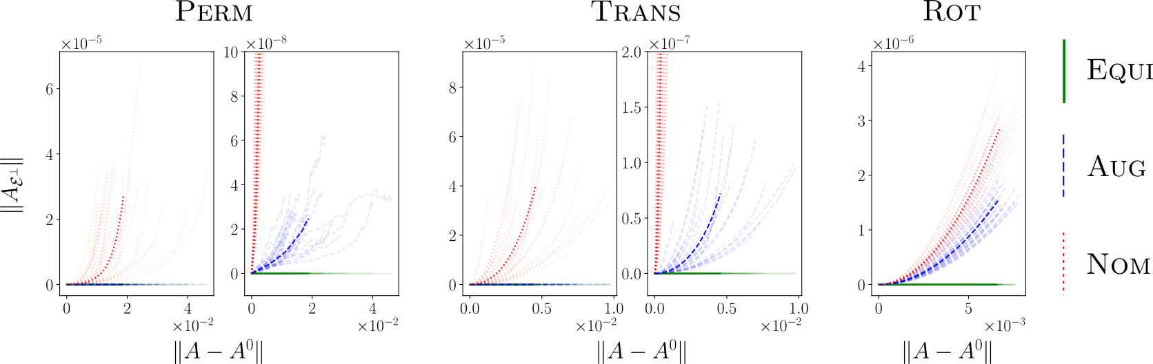
Figure 1: Results of the experiments: $\|A_{\mathcal{E}^{\perp}}\|$ is plotted versus $\|A-A^{0}\|$. Opaque lines are to mean values, transparent lines are individual experiments. For Perm and Trans , the two plots depict the same data with different scales on the $\|A_{\mathcal{E}^{\perp}}\|$-axis.

6 Conclusion

In this paper we investigated the dynamics of gradient descent for augmented and equivariant models, and how they are related. In particular, we showed that the models have the same set of equivariant stationary points, but that the stability of these points may differ. Furthermore, when initialized to the equivariant subspace $\mathcal{E}$, the dynamics of the augmented model is identical to that of the equivariant one. In a first order approximation, dynamics on $\mathcal{E}$ and $\mathcal{E}^{\perp}$ even decouple for the augmented models.

These findings have important practical implications for the two strategies for incorporating symmetries in the learning problem. The fact that their equivariant stationary points agree implies that there are no equivariant configurations that cannot be found using manifest equivariance. Hence, the more efficient parametrisation of the equivariant models neither introduces nor excludes equivariant stationary points compared to the less restrictive augmented approach. Conversely, if we can control the potential instability of the non-equivariant subspace $\mathcal{E}^{\perp}$ in the augmented gradient flow, it will find the same equivariant minima as its equivariant counterpart. One way to accomplish the latter would be to introduce a penalty proportional to $\|{A_{\mathcal{E}^{\perp}}}\|^{2}$ in the augmented risk.

This work is a first step towards properly understanding the effects of augmentation on the dynamics of gradient flows, but more research is needed. For instance, although we showed that the dynamics on $\mathcal{E}$ is identical for the augmented and equivariant models, and understand their behaviour near $\mathcal{E}$, our results say nothing about the dynamics away from $\mathcal{E}$ for the augmented model. Indeed, there is nothing stopping the augmented gradient flow from leaving $\mathcal{E}$ – although initialized very near it – or from coming back again. To analyse the global properties of the augmented gradient flow, in particular to calculate the spectra of $\nabla^{2}R^{\mathrm{aug}}$ in concrete cases of interest, is an important direction for future research.

Acknowledgement

This work was partially supported by the Wallenberg AI, Autonomous Systems and Software Program (WASP) funded by the Knut and Alice Wallenberg Foundation. The computations were enabled by resources provided by the National Academic Infrastructure for Supercomputing in Sweden (NAISS) at Chalmers University of Technology partially funded by the Swedish Research Council through grant agreement no. 2022-0672.

Appendix A Collected proofs of theoretical results

In this appendix, we collect proofs of the theoretical results that were not given in Section 3. Most of the claims are well-known, and we include them mainly to keep the article self-contained.

We begin by proving a small claim we will use implicitly throughout.

Lemma 7.

The lifted representations $\overline{\rho}_{i}$ on $\mathrm{Hom}(X_{i},X_{i+1})$, $\overline{\rho}$ on $\mathcal{L}$ and $\overline{\rho}^{\otimes 2}$ on $\mathcal{L}^{\otimes 2}$ are unitary with respect to the canonical inner products.

Proof.

Let us begin by quickly establishing that the $\overline{\rho}_{i}$ are representations:

$$\overline{\rho}_{i}(g)\overline{\rho}_{i}(h)A_{i}=\rho_{i+1}(g)\rho_{i+1}(h)A_{i}\rho_{i}(h)^{-1}\rho_{i}(g)^{-1}=\rho_{i+1}(gh)A_{i}\rho_{i}(gh)^{-1}=\overline{\rho}(gh)A_{i}$$ (28)

Now let us move on to the unitarity. We have

$$\langle\overline{\rho}_{i}(g)A_{i},\overline{\rho}_{i}(g)B_{i}\rangle =\mathrm{tr}((\rho_{i+1}(g)A_{i}\rho_{i}(g)^{-1})^{*}\rho_{i+1}(g)B_{i}\rho_{i}(g)^{-1})$$ (29)

$$=\mathrm{tr}(\rho_{i}(g)A_{i}^{*}\rho_{i+1}(g)^{-1}\rho_{i+1}(g)B_{i}\rho_{i}(g)^{-1})$$

$$=\mathrm{tr}(A_{i}^{*}B_{i}\rho_{i}(g)^{-1}\rho_{i}(g))=\mathrm{tr}(A_{i}^{*}B_{i})=\langle A_{i},B_{i}\rangle$$

which immediately implies

$$\langle\overline{\rho}(g)A,\overline{\rho}(g)B\rangle=\sum_{i\in[L]}\langle\overline{\rho}_{i}(g)A_{i},\overline{\rho}_{i}(g)B_{i}\rangle=\sum_{i\in[L]}\langle A_{i},B_{i}\rangle=\langle A,B\rangle$$ (30)

proving the unitarity of $\overline{\rho}_{i}$ and then $\overline{\rho}$. Unitary of $\overline{\rho}^{\otimes 2}$ then follows from the fundamental properties of the tensor product:

$$\langle\overline{\rho}^{\otimes 2}(g)(A\otimes B),\overline{\rho}^{\otimes 2}(g)(C\otimes D)\rangle =\langle(\overline{\rho}(g)A\otimes\overline{\rho}(g)B),(\overline{\rho}(g)C\otimes\overline{\rho}(g)D)\rangle$$ (31)

$$=\langle\overline{\rho}(g)A,\overline{\rho}(g)C\rangle\langle\overline{\rho}(g)B,\overline{\rho}(g)D\rangle=\langle A,C\rangle\langle B,D\rangle$$

$$=\langle(A\otimes B),(C\otimes D)\rangle\,.$$

∎

Next, we prove the lemmas concerning the lifted representation $\overline{\rho}$.

Proof of Lemma 1.

The statement follows immediately from the fact the a tuple of layers $A\in\mathcal{L}$ is in $\mathcal{E}$ if and only if $\rho_{i+1}(g)A_{i}=A_{i}\rho_{i}(g)$, which is equivalent to $A_{i}=\rho_{i+1}(g)A_{i}\rho_{i}(g)^{-1}=(\overline{\rho}(g)A)_{i}$ for all $i\in[L]$ and $g\in G$. ∎

Proof of Lemma 2.

Let $P$ be the operator on $\mathcal{L}$ defined by

$$PA=\int_{G}\overline{\rho}(g)A\,\mathrm{d}\mu(g).$$ (32)

To show that $P=\Pi_{\mathcal{E}}$, we first need to show that if $PA\in\mathcal{E}$ for any $A\in\mathcal{L}$. To do this, it suffices by Lemma 1 to prove that $\overline{\rho}(g)PA=PA$ for any $g\in G$. Using the fact that $\overline{\rho}$ is an representation of $G$, and the invariance of the Haar measure, we obtain

$$\overline{\rho}(g)PA=\int_{G}\overline{\rho}(g)\overline{\rho}(h)A\,\mathrm{d}\mu(h)=\int_{G}\overline{\rho}(gh)A\,\mathrm{d}\mu(h)=\int_{G}\overline{\rho}(h^{\prime})A\,\mathrm{d}\mu(h^{\prime})=PA.$$ (33)

Next, we need to show that $PA=A$ for any $A\in\mathcal{E}$. But since $\overline{\rho}(g)A=A$ for such $A$, we immediately obtain

$$PA=\int_{G}\overline{\rho}(g)A\,\mathrm{d}\mu(g)=\int_{G}A\,\mathrm{d}\mu(g)=A.$$ (34)

Consequently, $P:\mathcal{L}\to\mathcal{E}$ is a projection. Finally, to establish that $P$ is also orthogonal, we need to show that $\langle A-PA,B\rangle=0$ for all $A\in\mathcal{L}$, $B\in\mathcal{E}$. This is a simple consequence of the unitarity of $\overline{\rho}$ and Lemma 1,

$$\langle PA,B\rangle=\int_{G}\langle\overline{\rho}(g)A,B\rangle\,\mathrm{d}\mu(g)=\int_{G}\langle\overline{\rho}(g)A,\overline{\rho}(g)B\rangle\,\mathrm{d}\mu(g)=\int_{G}\langle A,B\rangle\,\mathrm{d}\mu(g)=\langle A,B\rangle\,,$$ (35)

which completes the proof that $P=\Pi_{\mathcal{E}}$. ∎

Proof of Lemma 5.

Replacing $\mathcal{L}$ with $\mathcal{L}\otimes\mathcal{L}$, $\mathcal{E}$ with $\mathcal{E}^{{\otimes 2}}$ and $\overline{\rho}$ with $\overline{\rho}^{{\otimes 2}}$, the proof is identical to that of Lemma 2. ∎

Proof of Lemma 6.

For $A\in\mathcal{E}$ we have $\overline{\rho}(g)A=A$ for any $g\in G$ according to Lemma 1. Consequently,

$$\left(\Pi_{\mathcal{E}^{\otimes 2}}M\right)[A,A] =\int_{G}\overline{\rho}^{{\otimes 2}}(g)M[A,A]d\mu(g)=\int_{G}M[\overline{\rho}(g)A,\overline{\rho}(g)A]d\mu(g)$$ (36)

$$=\int_{G}M[A,A]d\mu(g)=M[A,A]\,.$$ (37)

which proves the first statement. To prove the second, we use that for $B\in\mathcal{E}^{\perp}$, $\Pi_{\mathcal{E}}B=0$ by definition. A similar calculation as above now yields

$$\left(\Pi_{\mathcal{E}^{\otimes 2}}M\right)[A,B] =\int_{G}\overline{\rho}^{{\otimes 2}}(g)M[A,B]d\mu(g)=\int_{G}M[\overline{\rho}(g)A,\overline{\rho}(g)B]d\mu(g)$$ (38)

$$=\int_{G}M[A,\overline{\rho}(g)B]d\mu(g)=M[A,\Pi_{\mathcal{E}}B]=0\,,$$ (39)

where we have used the bilinearity of $M$ repeatedly to complete the proof. ∎

Appendix B Examples of representations

In addition to the examples provided in the main part of the paper, the following representations will feature in the experimental design described below.

Example 3.

The canonical action of the permutation group $S_{N}$ on $\mathbb{R}^{N}$ is defined through $(\rho^{\mathrm{perm}}(\pi)v)_{i}=v_{\pi^{-1}(i)},i\in[n]$, i.e., an element acts via permuting the elements of a vector. This action induces an action on the tensor space $(\mathbb{R}^{N})^{\otimes k}=\mathbb{R}^{N}\otimes\mathbb{R}^{N}\otimes\dots\otimes\mathbb{R}^{N}$: $(\rho^{\mathrm{perm}}(\pi)T)_{i_{0},\dots,i_{k-1}}=T_{\pi^{-1}(i_{0}),\dots,\pi^{-1}(i_{k-1})}$ which is important for graphs. For instance, when applied to $\mathbb{R}^{N}\otimes\mathbb{R}^{N}$, it encodes the effect a re-ordering of the nodes of a graph has on the adjacency matrix on the graph.

Example 4.

$C_{4}\cong\mathbb{Z}_{4}$ acts on images $x\in\mathbb{R}^{N,N}$ through rotations by multiples of $90^{\circ}$. That is, $\rho^{\mathrm{rot}}(k)=\rho^{\mathrm{rot}}(1)^{k}$, $k=0,1,2,3$ where $(\rho^{\mathrm{rot}}(1)x)_{i,j}=x_{-j,i}$.

Appendix C The converse of Proposition 3 does not hold

To construct a counterexample, it is clearly enough to construct $U\in\mathcal{L}\otimes\mathcal{L}$ such that $U$ is not positive definite but $\Pi_{\mathcal{E}^{\otimes 2}}U$, and $V\in\mathcal{E}^{\otimes 2}$ such that $V$ is not positive definite but $\Pi_{\mathcal{E}}^{\otimes 2}V$ is.

We choose $\mathcal{L}=\mathbb{R}^{N}$ and $G=S_{N}$ with the canonical representation $\overline{\rho}=\rho^{\mathrm{perm}}$ as in Example 3. With $e_{i}$, $i=1,\ldots,N$, the standard ONB of $\mathcal{L}$ we can construct the equivariant subspaces of $\mathcal{L}$ and $\mathcal{L}\otimes\mathcal{L}$ using

$$\mathds{1}=\sum_{i=1}^{N}e_{i}\in\mathcal{L}\,,\quad\mathrm{id}=\sum_{i=1}^{N}e_{i}\otimes e_{i}\in\mathcal{L}^{\otimes 2}$$ (40)

as $\mathcal{E}=\mathrm{Span}\{\mathds{1}\}$ and $\mathcal{E}^{\otimes 2}=\mathrm{Span}\{\mathrm{id},\mathds{1}\otimes\mathds{1}\}$ [22]. Furthermore, ONBs of the two spaces are given by

$$B_{\mathcal{E}}^{1}=\tfrac{1}{\sqrt{N}}\mathds{1}\qquad\text{and }B_{\mathcal{E}^{\otimes 2}}^{1}=\tfrac{1}{\sqrt{N}}\mathrm{id},B_{\mathcal{E}^{\otimes 2}}^{2}=\tfrac{1}{\sqrt{N(N-1)}}(\mathds{1}\otimes\mathds{1}-\mathrm{id})\,,$$

respectively.

Now consider the matrix $U=(N+1)e_{1}\otimes e_{1}-e_{2}\otimes e_{2}\in\mathcal{L}^{\otimes 2}$. It is not positive definite, since $U[e_{2},e_{2}]=-1$. However, as a direct calculation reveals, its projection to $\mathcal{E}^{\otimes 2}$, $\Pi_{\mathcal{E}^{\otimes 2}}U=\mathrm{id}$, clearly is.

Second, we can construct a matrix $V=-\mathrm{id}+\frac{2}{N}(\mathds{1}\otimes\mathds{1})\in\mathcal{E}^{\otimes 2}$ which is not positive definite, since its restriction to $\mathcal{E}^{\perp}$ is $-\mathrm{id}$. However, the projection $\Pi_{\mathcal{E}}^{\otimes 2}V=\tfrac{1}{N}\mathds{1}\otimes\mathds{1}$ is positive definite when restricted to $\mathcal{E}$.

Appendix D Experimental details

Here, we provide a more detailed description of the experiments in Section 5 in the main paper. Each experiment used a single NVIDIA Tesla T4 GPU with 16GB RAM, but many of them were performed in parallell on a cluster. The experiments presented here took in total about 75 GPU hours.

The code is provided at https://github.com/usinedepain/eq_aug_dyn.

D.1 The Perm experiment

In the Perm experiment, we train a model to detect whether a graph is connected or not. The model takes adjacency matrices $M\in\mathbb{R}^{N}\otimes\mathbb{R}^{N}$ of the graph as input. The training task is obviously invariant to permutations of the adjacency matrix (where the action of $S_{N}$ on the matrix space was defined in Example 3 in the main paper), since such a permutation does not change the underlying graph. The invariance of the network is conveniently expressed by letting $S_{N}$ acting trivially on the output space $Y=\mathbb{R}$.

Data

We consider graphs of size $N=10$ drawn according to a stochastic block model: We divide the nodes into two randomly drawn clusters $I,J$, $I\cap J=\emptyset$, $I\cup J=\{0,\dots,10\}$. Within each cluster, a bidirected edge is added between each pair of nodes with a probability of $0.5$, and in between the clusters with a probability of $0.05$. The graphs are subsequently checked for connectivity by checking that all entries of $\sum_{i=0}^{N}A^{i}$ are strictly positive, which clearly is sufficient. In this manner, we generate a $1000$ graphs and labels.

Model

The model set up is as follows: Before the first layer, the inputs are ’normalized’ by subtracting $.5$ from each entry. Then, the first layer is chosen to map from the input space $\mathbb{R}^{N}\otimes\mathbb{R}^{N}$ into another space of adjacency matrices matrices $(\mathbb{R}^{N}\otimes\mathbb{R}^{N})^{32}$, (on which $S_{N}$ is acting according to $\rho^{\mathrm{perm}}$, defined in Example 3, on each component). Then, a group pooling layer is used, that is, a map into $\mathbb{R}^{64}$ on which $S_{N}$ is acting trivially. This is followed by a layer normalization layer, and then two layers $\mathbb{R}^{64}\to\mathbb{R}^{32}$ and $\mathbb{R}^{32}\to\mathbb{R}$. The group acts trivially on each of the final spaces. In other words, all models are equipped a fully connected head. All but the last non-linearities are chosen as leaky ReLUs, whereas the last one is a sigmoid function. Note that the non-linearities are applied pointwise in the early layers, so that they are trivially equivariant to the group action. We use a binary loss. A graphical depiction of the architecture is given in Figure 2.

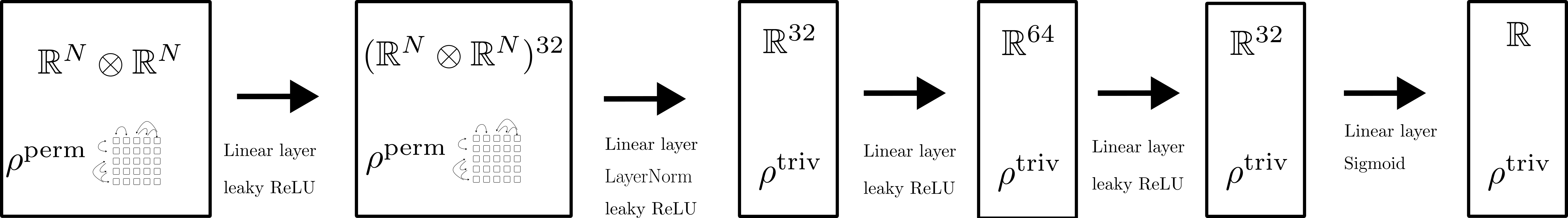
Figure 2: The setup for the models of Perm.

Projection operators

To project the layers onto $\mathcal{E}$, we use the results of [22]. In said paper, bases for the space invariant under the (lifted) representation $\rho^{\mathrm{perm}}$ on $(\mathbb{R}^{N})^{\otimes k}$ are given. In this context, the first layer consists of a $(32\times 1)$ array of elements in $(\mathbb{R}^{N}\otimes\mathbb{R}^{N})\otimes(\mathbb{R}^{N}\otimes\mathbb{R}^{N})=(\mathbb{R}^{N})^{\otimes 4}$, the second is an $(32\times 32)$ array of elements in $\mathbb{R}\otimes(\mathbb{R}^{N}\otimes\mathbb{R}^{N})=(\mathbb{R}^{N})^{\otimes 2}$, and the final ones are simply arrays of real numbers (and in particular, $\mathcal{E}$ is the entire space).

D.2 The Trans experiment

In the Trans experiment, we train a model for classification on MNIST. The input space here is $X_{0}=\mathbb{R}^{N,N}$, where $N$ is the width/height of the image. On $X_{0}$, we let the translation group $\mathbb{Z}_{N}^{2}$ act as in Example 2. The classification task is invariant to this action, whence we again let $\mathbb{Z}_{N}^{2}$ act trivially on the output space $\mathbb{R}^{10}$ of probability distribution on the ten classes.

Data

We use the public dataset MNIST [19] in our experiments, but modify it in two ways to keep the experiments light. First, we train our models only on the 10000 test examples (instead of the 60000 training samples). Secondly, we subsample the $28\times 28$ images to images of size $14\times 14$ (and hence set $N=14$) using opencv’s [4] built-in Resize function. This simply to reduce the size of the networks. Note that the size of the early (non-equivariant) layers of the model are proportional to the $(\text{image width})^{4}$.

Model

We again begin by ’normalizing’ the output by subtracting $.5$ from each pixels. The actual architecture then begins with two initial layers mapping between spaces on which $\mathbb{Z}_{N}^{2}$ acts according to $\rho^{\mathrm{tr}}$ (in each component) : Layer $1$ maps from $\mathbb{R}^{N,N}\to(\mathbb{R}^{N,N})^{32}$ and layer $2$ from $(\mathbb{R}^{N,N})^{32}$ to $(\mathbb{R}^{N,N})^{32}$. We then again apply a group pooling layer followed by a ’fully connected head’: The third layer maps into $\mathbb{R}^{32}$, on which $\mathbb{Z}_{N}^{2}$ is acting trivially, and the final one between $\mathbb{R}^{32}$ and $\mathbb{R}^{10}$. After the pooling layer, we add a layer normalization layer. The non-linearities are again chosen as leaky ReLU:s, except for the last one, which is a SoftMax. The equivariance of the non-linearities are again lifted from them acting elementwise on the first three spaces. We use a cross-entropy loss. A graphical depiction of the setup is given in 3.

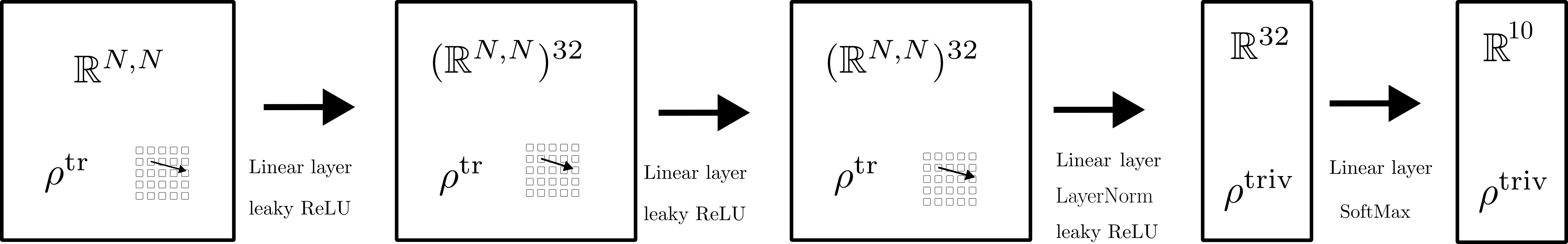
Figure 3: The setup for the models of Trans.

Projection operators

It is well-known that a linear operator on $\mathbb{R}^{N,N}$ is equivariant if and only if it is a convolutional operator. Hence, for the first two layers, the projection is carried out via projecting each component onto the space spanned by

$$C^{k\ell}=\sum_{i,j\in[N]}(e_{i}\otimes e_{j})\otimes(e_{i+k}\otimes e_{i+\ell}),\quad k,\ell\in[N]^{2}.$$ (41)

The third layers consist of arrays of functionals on $\mathbb{R}^{N,N}$. The only linear invariant such is (up to scale and interpreted as a member of $\mathbb{R}^{N,N}$) the constant matrix. Hence, the projection in this space simply consists of averaging the layer. After that, just as above, $\mathcal{E}$ is the entire space, and the projection is trivial.

The convolution operators are furthermore well-known to be characterized as diagonal operators in the Fourier domain. We may therefore implement the projection onto $\mathcal{E}$ efficiently by first transforming into Fourier domain, extract the diagonal, and then transforming back. For completeness, let us quickly prove that this really yields the orthogonal projection.

Proposition 4.

For $N\in\mathbb{N}$, let the translation group $G=\mathbb{Z}_{N}^{2}$ act on the space $\mathbb{C}^{N,N}\sim\mathbb{C}^{[N]^{2}}$. If we let $\mathcal{F}:\mathbb{C}^{N,N}\to\mathbb{C}^{N,N}$ denote the orthogonal two-dimensional Fourier transform, and $\mathrm{diag}:\mathbb{C}^{N,N}\to\mathbb{C}^{N,N}$ the operator that kills all off-diagonal values, the orthogonal projection onto $\mathrm{Hom}_{G}(\mathbb{C}^{N,N},\mathbb{C}^{N,N})$ is given by

$$\Pi_{\mathcal{E}}(A)=\mathcal{F}^{-1}\mathrm{diag}(\mathcal{F}A\mathcal{F}^{-1})\mathcal{F}.$$ (42)

Proof.

Let us begin by showing that $P=\mathcal{F}^{-1}\mathrm{diag}(\mathcal{F}A\mathcal{F}^{-1})\mathcal{F}$ defines an orthogonal projection. As for the ’projection’ part, note that for any $A$, the matrix $D=\mathrm{diag}(\mathcal{F}A\mathcal{F}^{-1})$ will of course be diagonal, so that $\mathrm{diag}(D)=D$. Consequently,

$$P^{2}(A)=P(\mathcal{F}^{-1}D\mathcal{F})=\mathcal{F}^{-1}\mathrm{diag}(D)\mathcal{F}=\mathcal{F}^{-1}D\mathcal{F}=P(A).$$ (43)

The orthogonality can now be shown via arguing that $P$ is self-adjoint. This is furthermore not hard: Due to the orthogonality of $\mathcal{F}$, $A\mapsto\mathcal{F}A\mathcal{F}^{-1}$ and $A\mapsto\mathcal{F}^{-1}A\mathcal{F}$ are self-adjoint, as is obviously $\mathrm{diag}$ (with respect to the standard scalar product on $\mathbb{C}^{N,N}$).

It is now only left to show that the range of $P$ is equal to the space $\mathrm{Hom}_{G}(\mathbb{C}^{N,N},\mathbb{C}^{N,N})$, which is the space of translations equivariant operators $\mathbb{C}^{N,N}\to\mathbb{C}^{N,N}$. It is however well-known that those exactly correspond to convolutional operators $C_{\phi}(v)=\phi*v$. The convolution theorem now states

$$\mathcal{F}(C_{\phi}v)=\mathcal{F}(\phi*v)=\mathcal{F}(\phi)\cdot\mathcal{F}(v)=\mathcal{D}(\mathcal{F}(\phi))\mathcal{F}v,$$ (44)

where $\mathcal{D}:\mathbb{C}^{N}\mapsto\mathbb{C}^{N,N}$ is the operator that inserts a vector into the diagonal of a matrix. In other words, $C_{\phi}=\mathcal{F}^{-1}\mathcal{D}(\mathcal{F}(\phi))\mathcal{F}$, which makes it obvious that $\mathrm{ran}P\subseteq\mathcal{E}$. Furthermore, by setting $A=\mathcal{F}^{-1}\mathcal{D}(\mathcal{F}(\phi))\mathcal{F}$, we see that we can write every convolution operator as an image under $P$. In conclusion, $P=\Pi_{\mathcal{E}}$.

∎

D.3 The Rot experiment

In the final experiment, we consider a simple, rotation invariant, segmentation task for synthetically generated data. The input space consist of images in $\mathbb{R}^{N,N}$, and the output space $(\mathbb{R}^{N,N})^{2}$ of pairs of segmentation masks. This task is hence ’truly’ equivariant.

Data

We generate $3000$ synthetic images as follows: With equal probability, we generate a regular pentagon or an equilateral triangle (with vertices on the unit circle), scale it using a uniformly randomly chosen factor in $[0.7,0.8]$, and place it randomly on a canvas. The resulting image, along with two segmentation masks, each indicating where each shape is present in the image (and in particular zero everywhere if the particular object is not present at all) are converted to $14\times 14$ pixels images. Importantly, all triangles, and pentagons, have the same orientation, so that the image distribution is not invariant under discrete rotations of $90^{\circ}$. Examples of generated images are showcased in Figure 4.

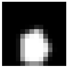
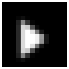
Figure 4: Two examples of generated images for Rot.

Model

In contrast to the previous examples, the action on the output space is not trivial. Therefore, the model set up is less convoluted : We use hidden spaces $(\mathbb{R}^{N,N})^{32}$,$(\mathbb{R}^{N,N})^{32}$ and $(\mathbb{R}^{N,N})^{16}$ on which the rotation group acts according to $\rho^{\mathrm{rot}}$ (on each component). Before the final non-linearity, we use a batch norm layer. All non-linearities are leaky ReLUs, except for the last one, which is a sigmoid non-linearity. A visualization is given in Figure 5. The loss function is

$$\ell((y_{\mathrm{pent}},y_{\mathrm{tri}}),y_{\mathrm{pent}}^{\prime},y_{\mathrm{tri}}^{\prime})=\frac{1}{N^{2}} \sum_{k\in[N]^{2}}\mathrm{BCL}((y_{\mathrm{pent}}(k),y_{\mathrm{pent}}^{\prime}(k)))$$ (45)

$$+\frac{1}{N^{2}}\sum_{k\in[N]^{2}}\mathrm{BCL}(y_{\mathrm{tri}}(k),y_{\mathrm{tri}}^{\prime}(k)))$$

where $\mathrm{BCL}$ is the binary cross-entropy loss, and $y_{\mathrm{pent}}$, $y_{\mathrm{tri}}$ are the pentagon and triangle segmentation masks, respectively. Note that the pixel-wise nature of the loss implies that it is invariant under rotations of the masks.

Projection operators

Since the group in this case only consists of four elements, and the Haar measure is the uniform one, we can calculate the projection of the layers by explicitly carrying out the integration

$$\Pi_{\mathcal{E}}A=\tfrac{1}{4}\sum_{k\in\mathbb{Z}_{4}}\overline{\rho}(k)A.$$ (46)

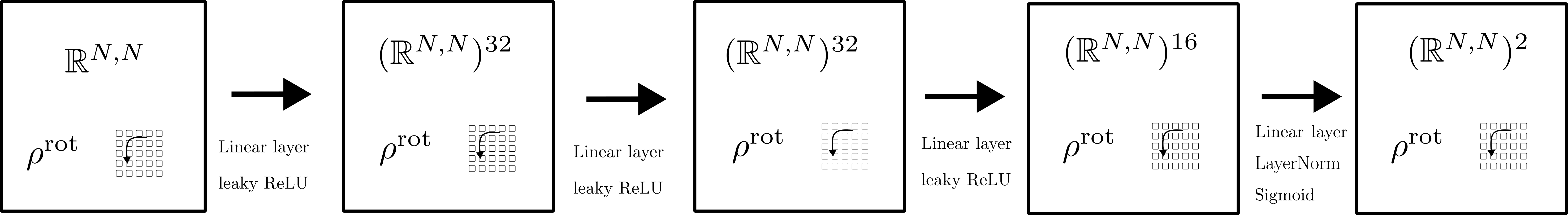
Figure 5: The setup for the models of Experiment 3

Appendix E The relation between $\dim(\mathcal{E})$ and the ’empirical stability’ of $\mathcal{E}$.

Experiment	$U$	$V$	$\dim\mathrm{Hom}(U,V)$	$\dim\mathrm{Hom}_{G}(U,V)$	# in model
Perm	$\mathbb{R}^{N}\otimes\mathbb{R}^{N}$	$\mathbb{R}^{N}\otimes\mathbb{R}^{N}$	$N^{4}$	15	32
	$\mathbb{R}^{N}\otimes\mathbb{R}^{N}$	$\mathbb{R}$	$N^{2}$	$2$	$32\cdot 64$
	$\mathbb{R}$	$\mathbb{R}$	1	1	$64\cdot 32+32\cdot 1$
Trans	$\mathbb{R}^{N,N}$	$\mathbb{R}^{N,N}$	$N^{4}$	$N^{2}$	$32+32\cdot 32$
	$\mathbb{R}^{N,N}$	$\mathbb{R}$	$N^{2}$	1	$32\cdot 32$
	$\mathbb{R}$	$\mathbb{R}$	1	1	$32\cdot 10$
Rot	$\mathbb{R}^{N,N}$	$\mathbb{R}^{N,N}$	$N^{4}$	$\tfrac{1}{4}\cdot N^{4}$	$32+32\cdot 32+$
					$32\cdot 16+16\cdot 2$

Table 1: Dimension calculations for the experiments Perm , Trans and Rot from the main paper.

In the main text, we sketched a heuristic argument relating the relative dimension of the space $\mathcal{E}$ in the space $\mathcal{L}$ with how close the Aug model stayed to $\mathcal{E}$. In this section, we first want to carry out these computations. To further investigate the link, we also provide an additional experiment. A quick glance of the calculations are given in Tables 1 and 2

E.1 The experiments in Section 5

Perm

As mentioned before, the spaces of equivariant linear maps was described in [22]. Therein, it was shown that the dimension of (under the permutation group) equivariant linear maps from $\mathbb{R}^{N}\otimes\mathbb{R}^{N}$ to itself is equal to $15$, and from $\mathbb{R}^{N}\otimes\mathbb{R}^{N}$ to itself is $2$ (as long as $N\geq 2$, as was pointed out in [13]). The dimensions of the corresponding whole spaces are $N^{4}$ and $N^{2}$, respectively. In the architecture we are proposing, we use $32$ maps $\mathbb{R}^{N}\otimes\mathbb{R}^{N}$ in the first layer, and $32\cdot 64$ maps $\mathbb{R}^{N}\otimes\mathbb{R}^{N}\to\mathbb{R}$ in the second layer. In the layers thereafter, all $64\cdot 32+32\cdot 1$ maps are equivariant. Hence

$$\frac{\dim\mathcal{E}}{\dim\mathcal{L}}=\frac{15\cdot 32+5\cdot 32\cdot 64+64\cdot 32+32\cdot 1}{N^{4}\cdot 32+N^{2}\cdot 32\cdot 64+64\cdot 32+32\cdot 1}\approx 2.43\cdot 10^{-2}.$$ (47)

where we plugged in $N=10$ in the final step.

Trans

Here, the space of equivariant linear maps $\mathbb{R}^{N,N}\to\mathbb{R}^{N,N}$ is the space of convolution operators. On $\mathbb{R}^{N,N}$, there are $N^{2}$ of those. There is up to scale only one equivariant map $\mathbb{R}^{N,N}\to\mathbb{R}$, given by taking the mean of the matrix entries. The space of all linear maps in the two cases of course have dimension $N^{4}$ and $N^{2}$, respectively. Since we use two initial layers of $32$ and $32\cdot 32$ maps $\mathbb{R}^{N,N}\to\mathbb{R}^{N,N}$, respectively, one layer of $32\times 32$ maps $\mathbb{R}^{N,N}\to\mathbb{R}$ and $32\cdot 10$ maps from $\mathbb{R}\to\mathbb{R}$ (where again all maps are equivariant), we obtain

$$\frac{\dim\mathcal{E}}{\dim\mathcal{L}}=\frac{N^{2}\cdot 32+N^{2}\cdot 32\cdot 32+1\cdot 32\cdot 32+32\cdot 10}{N^{4}\cdot 32+N^{4}\cdot 32\cdot 32+N^{2}\cdot 32\cdot 32+32\cdot 10}\approx 5.1\cdot 10^{-3}.$$ (48)

where we plugged in $N=14$ in the final step.

Rot

Here, a map from $\mathbb{R}^{N,N}$ to $\mathbb{R}^{N,N}$ is clearly equivariant if and only if its matrix representation, as a function from $([N]^{2})^{2}$ to $R$, is constant along all orbits

$$\{(\iota_{0},\iota_{1}),(r^{-1}(\iota_{0}),r(\iota_{1})),(r^{-2}(\iota_{0}),r^{2}(\iota_{1})),(r^{-3}(\iota_{0}),r^{3}(\iota_{1}))\},$$ (49)

where $\iota_{i}=[\iota_{i}(0),\iota_{i}(1)]\in[N]^{2}$ and

$$r(\iota)=(-\iota(1),\iota(0))$$ (50)

Since $N=14$, i.e. even, each such orbit has $4$ elements, and they are of course disjoint. Therefore, the relative dimension between the space of equivariant maps $\mathbb{R}^{N,N}\to\mathbb{R}^{N,N}$ and the space of all such maps is equal to $1/4$. Since it is only such maps that appear in the model used in the experiment,

$$\frac{\dim\mathcal{E}}{\dim\mathcal{L}}=\frac{1}{4}=0.25$$ (51)

in this case.

E.2 An additional experiment

In the main paper, not only $G$ (and accordingly $\mathcal{E}$) was varying in between the experiment, but also the nominal model architectures and datasets, which makes it unclear if it is only $G$ that plays a role in the different speeds of drift of the augmented model from (or say ’empirical stability’ of) $\mathcal{E}$ . We therefore perform an additional experiment in which all models use the same underlying architecture and dataset, namely the one of the Trans experiment, and only vary the underlying symmetry group acting on $\mathbb{R}^{N,N}$. We use four groups and actions.

• Trans  $\mathbb{Z}_{N}^{2}$ acting through translations, as in the Trans experiment.

• Rot $\mathbb{Z}_{4}$ acting through rotations, as in the Rot experiment.

• OneDTrans $\mathbb{Z}_{N}$ acting through translations in the $x$-direction, i.e.

  $$(\rho^{\mathrm{tr}_{0}}(k)x)_{i,j}=x_{i-k,j}$$ (52)

• TransRot The semi-direct product $\mathbb{Z}_{N}^{2}\rtimes\mathbb{Z}^{4}$ acting through

  $$\rho^{\mathrm{trot}}(\iota,k)x=\rho^{\mathrm{rot}}(k)\rho^{\mathrm{tr}}(\iota)x,\quad\iota\in\mathbb{Z}_{N}^{2},k\in\mathbb{Z}_{4}.$$ (53)

  This can, in the same way $\mathbb{Z}_{4}$ is a discretization of the full group $\mathrm{SO}(2)$ of rotations in the plane, be thought of as a discretization of the group $\mathrm{SE}(2)$ of isometries in the plane.

The relative dimensions $\dim\mathcal{E}/\dim\mathcal{L}$ are in these cases (approximately) given by

$$\begin{tabular}[]{lllll }{Trans}~{}:&$5.1\cdot 10^{-3}$&&{Rot}~{}:&$0.25$\\ {OneDTrans}~{}:&$7.1\cdot 10^{-2}$&&{TransRot}~{}:&$1.3\cdot 10^{-3}$\end{tabular}.$$ (56)

These numbers are the results of similar calculations as above, with the data from Table (2) – the (conceptually simple but technical) arguments for the validity of non-trivial entries are given in Section E.2.1. According to it, we expect the relative drift of the augmented model compared to the nominal one from $\mathcal{E}$ should be the largest for Rot, followed by OneDTrans, Trans and TransRot, in decreasing order.

Experiment	$U$	$V$	$\dim\mathrm{Hom}(U,V)$	$\dim\mathrm{Hom}_{G}(U,V)$	# in model
Rot	$\mathbb{R}^{N,N}$	$\mathbb{R}^{N,N}$	$N^{4}$	$\tfrac{1}{4}N^{4}$	$32+32\cdot 32$
	$\mathbb{R}^{N,N}$	$\mathbb{R}$	$N^{2}$	$\tfrac{1}{4}N^{2}$	$32\cdot 32$
	$\mathbb{R}$	$\mathbb{R}$	1	1	$32\cdot 10$
OneDTrans	$\mathbb{R}^{N,N}$	$\mathbb{R}^{N,N}$	$N^{4}$	$N^{3}$	$32+32\cdot 32$
	$\mathbb{R}^{N,N}$	$\mathbb{R}$	$N^{2}$	$N$	$32\cdot 32$
	$\mathbb{R}$	$\mathbb{R}$	1	1	$32\cdot 10$
TransRot	$\mathbb{R}^{N,N}$	$\mathbb{R}^{N,N}$	$N^{4}$	$\tfrac{1}{4}N^{2}$	$32+32\cdot 32$
	$\mathbb{R}^{N,N}$	$\mathbb{R}$	$N^{2}$	1	$32+32\cdot 32$
	$\mathbb{R}$	$\mathbb{R}$	1	1	$32\cdot 10$

Table 2: Dimension calculations for the experiments Rot , OneDTrans and TransRot in the appendix.

As mentioned, we repeat the exact same experiment as Trans for the new groups. We then plot the results similarly as in the experiments in the main paper, in Figure 6. Note that the scales in the figures are different, to assess the amount the augmented model drifts relative to the other ones. We have chosen the limits for the axes as follows:

• The $x_{\mathrm{left}}$-limit in both subplots is chosen as $1.5$ times the maximal (with respect to the $50$ training epochs) median (with respect to the $30$ runs) value of $\|{A-A_{0}}\|$ for the Equi model.

• The $y_{\mathrm{left}}$-limit in the left subplot is chosen as $1.5$ times the maximal (with respect to the $50$ training epochs) median (with respect to the $30$ runs) value of $\|\Pi_{\mathcal{E}^{\perp}}A\|$ for the Nom model.

• The $y_{\mathrm{right}}$-limit in the left subplot is given by $\lambda\cdot y_{\mathrm{left}}$, where $\lambda>0$ is a factor common for all four groups. $\lambda$ is chosen so that $y_{\mathrm{right}}$ is equal to $1.5$ times the maximal (with respect to the $50$ training epochs) median (with respect to the $30$ runs) value of $\|{\Pi_{\mathcal{E}^{\perp}}A}\|$ for the Aug model for the Trans  experiment.

In this way, we ensure that the coordinate systems are on the same scale relative to the Nom and Equi models. It is hence not surprising that the Nom  curves look the same in all the plots – it is very much that way by design. The same is however not true for the Aug  curve, and that is telling us something – in fact, this behaviour is in accordance with our hypothesis. This further strengthens the argument that the dimension of the subspace $\mathcal{E}$ plays a crucial role in the amount of regularizing effect augmentation has. Judging by the quite small difference between Trans and TransRot , although the relative dimensions differ by a factor $4$, further suggests that hypothesizing a simple linear relationship is to naive – more work needs to be done here.

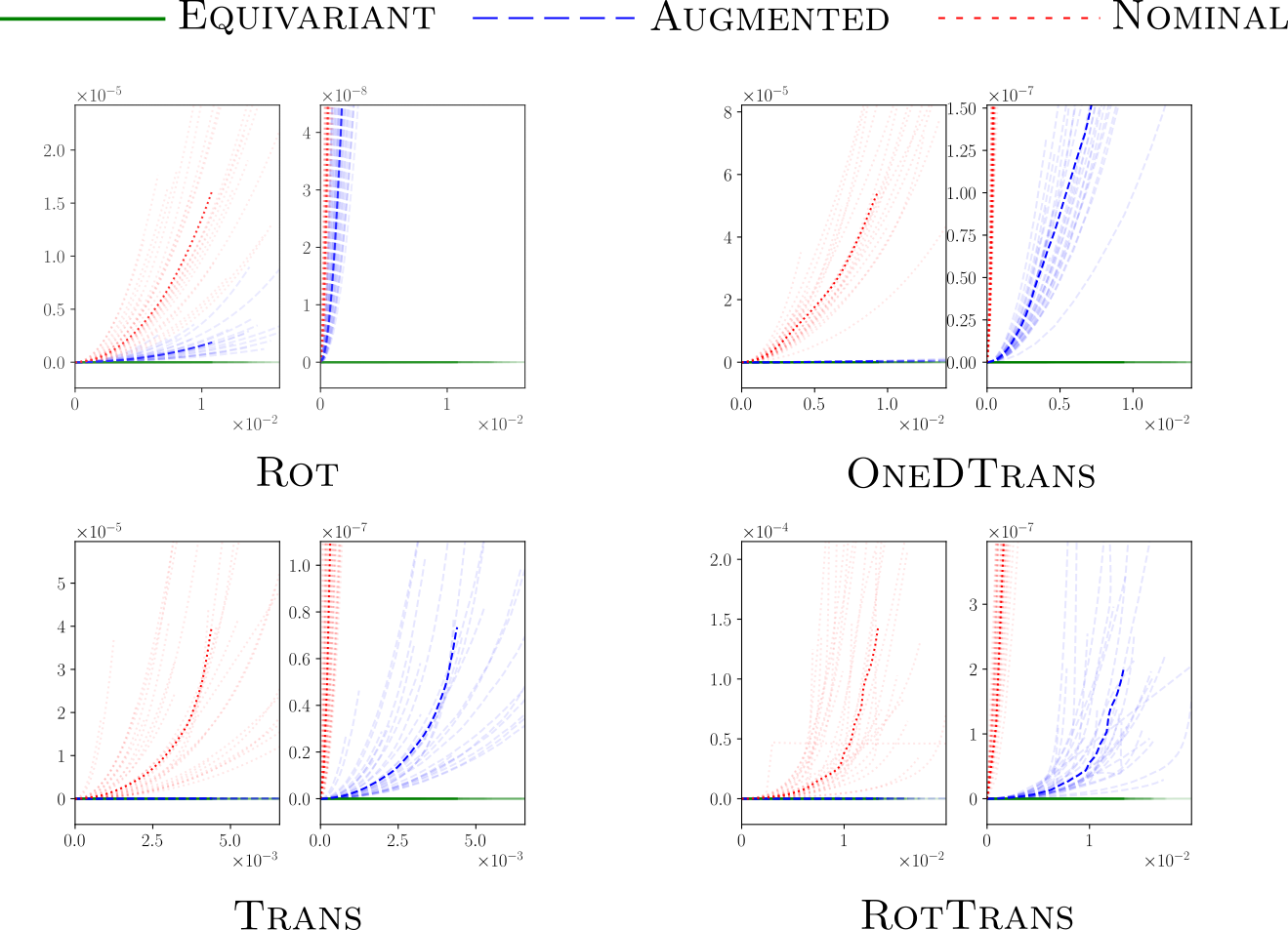
Figure 6: Results from the experiments of the appendix.

E.2.1 The spaces $\mathrm{Hom}_{G}(U,V)$ and projection operators

Here, we derive what $\mathrm{Hom}_{G}(U,V)$ look like for the groups $\mathbb{Z}_{N}$ and $\mathbb{Z}^{4}\rtimes\mathbb{Z}_{N}$, and the corresponding projection operators. These derivations are all conceptually easy, but technical, and are only included for completeness.

$\mathbb{Z}_{N}$ and OneDTrans 

To describe the space $\mathrm{Hom}_{\mathbb{Z}_{N}}(\mathbb{R}^{N,N},\mathbb{R}^{N,N})$, let us begin by introducing some notation. First, every element in $\mathbb{R}^{N,N}$ can equivalently be described as a collection of rows. This can be written compactly as

$$X=\sum_{k\in[N]}e_{k}x_{k}^{*}$$ (57)

where $x_{k}\in\mathbb{R}^{N}$ are the rows, and $e_{k}$ is the $k$:th canonical unit vector. Correspondingly, each operator $A:\mathbb{R}^{N,N}\to\mathbb{R}^{N,N}$ decomposes into an array of $N^{2}$ operators $A_{\ell,k}:\mathbb{R}^{N}\to\mathbb{R}^{N}$:

$$A(x)=\sum_{k,\ell\in[N]}e_{\ell}(A_{\ell,k}x_{k})^{*}.$$ (58)

With this notation introduced, we can conveniently describe the space $\mathrm{Hom}_{\mathbb{Z}_{N}}(\mathbb{R}^{N,N},\mathbb{R}^{N,N})$

Proposition 5.

Using the notation (58), $\mathrm{Hom}_{\mathbb{Z}_{N}}(\mathbb{R}^{N,N},\mathbb{R}^{N,N})$ is characterized as the set of operators for which each $A_{\ell,k}$ is a convolutional operator. In particular, the dimension of the space is $N^{2}\cdot N=N^{3}$.

Proof.

Somewhat abusing notation, let us denote the action of $\mathbb{Z}_{N}$ on $\mathbb{R}^{N}$ also as $\rho^{\mathrm{tr}_{0}}$. We then have

$$\rho^{\mathrm{tr}_{0}}(n)(e_{k}x^{*})=e_{k}\rho^{\mathrm{tr}_{0}}(n)(x)^{*}$$ (59)

Hence,

$$A(\rho^{tr_{0}}(n)x)=\sum_{k,\ell\in[N]}e_{\ell}(A_{\ell,k}\rho^{\mathrm{tr}_{0}}(n)x_{k})^{*}$$ (60)

$$\rho^{\mathrm{tr}_{0}(n)}(Ax)=\sum_{k,\ell\in[N]}e_{\ell}(\rho^{\mathrm{tr}_{0}}(n)A_{\ell,k}x_{k})^{*}$$ (61)

These two expression are equal for any $x$ if and only if $A_{\ell,k}\rho^{\mathrm{tr}_{0}}(n)x_{k}=\rho^{\mathrm{tr}_{0}}(n)A_{\ell,k}x_{k}$ for any $x_{k}$ and $\ell,k$, i.e., when every $A_{\ell,k}$ is translation equivariant, which is equivalent to each $A_{\ell,k}$ being a convolution operator. ∎

Not surprisingly, we can again calculate the projection onto the space of equivariant operators with the help of the Fourier transform. However, the Fourier transform should here only be applied partially. Let us make this explicit. Let $\mathcal{F}:\mathbb{C}^{N}\to\mathbb{C}^{N}$ be the one-dimensional orthogonal Fourier transform. We then define the row-wise partial Fourier transformation $\mathbb{F}:\mathbb{C}^{N,N}\to\mathbb{C}^{N,N}$ through

$$\mathbb{F}\left(\sum_{k\in[N]}e_{k}x_{k}^{*}\right)=\sum_{k\in\mathbb{N}}e_{k}(\mathcal{F}x_{k})^{*}.$$ (62)

We can now show that $A\in\mathrm{Hom}_{\mathbb{Z}^{N}}(\mathbb{C}^{N,N},\mathbb{C}^{N,N})$ is related to $\mathbb{F}A\mathbb{F}^{-1}$ being ’partially diagonal’, in the following sense.

Lemma 8.

Let $\mathcal{F}:\mathbb{C}^{N}\to\mathbb{C}^{N}$ be the one-dimensional Fourier transform. Then, an operator $A$ is in $\mathrm{Hom}_{\mathbb{Z}^{N}}(\mathbb{C}^{N,N},\mathbb{C}^{N,N})$ if and only if, in the notation 58, each $\mathcal{F}A_{\ell,k}\mathcal{F}^{-1}$ is diagonal.

Proof.

It is not hard to show that

$$(\mathbb{F}A\mathbb{F}^{-1})_{\ell,k}=\mathcal{F}A_{\ell,k}\mathcal{F}^{-1}.$$ (63)

Now, it is well known that $A_{\ell,k}$ is convolutional if and only if $\mathcal{F}A_{\ell,k}\mathcal{F}^{-1}$ is diagonal. The claim follows. ∎

By applying exactly the same argument as in Proposition 4, we may now derive

Proposition 6.

The orthogonal projection from $\mathrm{Hom}(\mathbb{C}^{N,N},\mathbb{C}^{N,N})$ onto $\mathrm{Hom}_{\mathbb{Z}^{N}}(\mathbb{C}^{N,N},\mathbb{C}^{N,N})$ is given by

$$\mathbb{F}^{-1}\mathrm{diag}_{0}(\mathbb{F}A\mathbb{F}^{-1})\mathbb{F},$$ (64)

where $\mathrm{diag}_{0}$ is the operator that kills all off-diagonal elements in all operators $A_{\ell,k}$ in the decomposition 58.

As before, it is not hard to realize what the space $\mathrm{Hom}_{\mathbb{Z}^{N}}(\mathbb{R}^{N,N},1)$ must be: Interpreted as a matrix $X=\sum_{k\in[N]}e_{k}x_{k}^{*}$, $X$ is in $\mathrm{Hom}_{\mathbb{Z}^{N}}(\mathbb{R}^{N,N},1)$ if and only if each $x_{k}$ is constant. Correspondingly, the projection is given by taking means along the $x$-direction, and the dimension of the space in particular is $N$.

$\mathbb{Z}_{4}$ and Rot 

Here, we have in fact already described the space $\mathrm{Hom}_{\mathbb{Z}_{4}}(\mathbb{R}^{N,N},\mathbb{R}^{N,N})$ and the projection operator in Appendix D. Let us here just record that the exact same idea goes through for the space $\mathrm{Hom}_{\mathbb{Z}_{4}}(\mathbb{R}^{N,N},1)$ – the projection can again be calculated via explicit integration, and its elements are again characterized by having constant values on orbits of length $4$. Correspondingly, $\dim\mathrm{Hom}_{\mathbb{Z}_{4}}(\mathbb{R}^{N,N},1)=\tfrac{1}{4}N^{2}$

TransRot  and $\mathbb{Z}_{N}^{2}\rtimes\mathbb{Z}_{4}$

Here, the semi-direct product structure immediately implies a relationship between the projection operators. First, let us notice that the lift $\overline{\rho}^{\mathrm{trot}}$ is given by $\overline{\rho}^{\mathrm{trot}}(\iota,k)=\overline{\rho}^{\mathrm{rot}}(k)\overline{\rho}^{\mathrm{tr}}(\iota)$. This fact together with the explicit integration formula

$$\Pi_{\mathcal{E}}=\int_{\mathbb{Z}_{N}^{2}\rtimes\mathbb{Z}_{4}}\overline{\rho}^{\mathrm{trot}}(g)\mathrm{d}\mu(g)=\frac{1}{4N^{2}}\sum_{k\in Z_{4},\iota\in\mathbb{Z}_{N}^{2}}\overline{\rho}^{\mathrm{rot}}(k)\overline{\rho}^{\mathrm{tr}}(\iota),$$ (65)

where we explicitly used that the Haar measure is the uniform one, implies the following

Proposition 7.

For $G$, let $P_{G}$ denote the projection operators onto $\mathrm{Hom}_{G}(\mathbb{R}^{N,N},V)$ where $V$ is either $\mathbb{R}$ or $\mathbb{R}^{N,N}$. Then,

$$P_{\mathbb{Z}_{N}^{2}\rtimes\mathbb{Z}^{4}}=P_{\mathbb{Z}_{4}}P_{\mathbb{Z}_{N}^{2}}.$$ (66)

The above in particular means that the space $\mathcal{E}$ is the intersection between the space $\mathcal{E}$ for the respective groups. Specifically, this means that the space $\mathrm{Hom}_{\mathbb{Z}_{N}\rtimes\mathbb{Z}_{4}}(\mathbb{R}^{N,N},\mathbb{R}^{N,N})$ is the space of convolution operators whose convolutional filter is constant on orbits under $\mathbb{Z}_{4}$, and therefore (in the even case) has dimension $\frac{N^{2}}{4}$. For $\mathrm{Hom}_{\mathbb{Z}_{N}\rtimes\mathbb{Z}_{4}}(\mathbb{R}^{N,N},\mathbb{R})$, the space is still one-dimensional – it is given by the convolution with the constant filter (which in particular is constant on orbits)..¨

Appendix F Including bias terms in the framework

Let us here show how bias terms can be incorporated into our framework by applying the standard trick of writing an affine map as a linear one on an extended space. Indeed, given an affine map $D:U\to V,x\mapsto Ax+b$ for some $A\in\mathrm{Hom}(U,V)$ and $b\in V$, we may define a linear map $D^{\circ}:U^{\circ}\to V^{\circ}$, where for a vector space $X$, we wrote $X^{\circ}=X\oplus\mathbb{R}$, through

$$D^{\circ}(x,\lambda)=(Ax+\lambda\cdot b,\lambda).$$ (67)

Note that $D^{\circ}(x,1)=(D(x),1)$. Hence, $D^{\circ}$ restricted to $U\times\{1\}$ acts exactly as $D$. These maps form a linear space that we call $\mathrm{Hom}^{\circ}(U^{\circ},V^{\circ})$. We can further extend a representation $\rho$ of $G$ on $U$ to one on $U^{\circ}$ via $\rho^{\circ}(g)(u,\lambda)=(\rho(g)u,\lambda)$. If $\rho$ is unitary, $\rho^{\circ}$ also is.

It is not hard to show that the affine map $D:X_{i}\to X_{i+1}$ is equivariant with respect to $\rho_{i},\rho_{i+1}$ if and only if the linear map $D^{\circ}$ is equivariant with respect to $\rho_{i}^{\circ}$, $\rho_{i+1}^{\circ}$. In particular, the lifted representation $\overline{\rho}_{i}^{\circ}$ maps $\mathrm{Hom}^{\circ}(X^{i},X^{i+1})$ onto itself, and $D^{\circ}$ is equivariant if and only if $\overline{\rho}(g)D^{\circ}=D^{\circ}$ for all $g$. Finally, the non-linearities $\sigma_{i}$ and loss $\ell$ can be extended to $\sigma_{i}^{\circ}:X_{i}^{\circ}\to X_{i+1}^{\circ},(x,\lambda)\to(\sigma(x),\lambda)$, and $\ell:Y^{\circ}\times Y^{\circ}\to R$, $\ell^{\circ}((x,\lambda),(y,\kappa))=\ell(x,y)$. Equivariance of $\sigma_{i}$ and $\ell$ is equivalent to equivariance of $\sigma^{\circ}$ and $\ell^{\circ}$, respectively.

Hence, in short, by extending all hidden spaces $X_{i}$ to $X_{i}^{\circ}$, the non-linearities, losses and representations accordingly, and restricting the $A_{i}$ to live in $\mathrm{Hom}^{\circ}(X_{i}^{\circ},X_{i+1}^{\circ})$, we obtain a framework that for all intents and purposes works exactly like the one we study in this paper, but also allows for the inclusion of bias terms. All arguments in the paper carry over verbatim in this extended framework.

References

- Aronsson [2022] Jimmy Aronsson. Homogeneous vector bundles and G-equivariant convolutional neural networks. Sampling Theory, Signal Processing, and Data Analysis, 20(10), 2022.
- Ba et al. [2016] Jimmy Lei Ba, Jamie Ryan Kiros, and Geoffrey E Hinton. Layer normalization. arXiv preprint arXiv:1607.06450, 2016.
- Bah et al. [2022] Bubacarr Bah, Holger Rauhut, Ulrich Terstiege, and Michael Westdickenberg. Learning deep linear neural networks: Riemannian gradient flows and convergence to global minimizers. Information and Inference: A Journal of the IMA, 11(1):307–353, 2022.
- Bradski [2000] G. Bradski. The OpenCV Library. Dr. Dobb’s Journal of Software Tools, 2000.
- Bronstein et al. [2017] Michael M Bronstein, Joan Bruna, Yann LeCun, Arthur Szlam, and Pierre Vandergheynst. Geometric deep learning: going beyond euclidean data. IEEE Signal Processing Magazine, 34(4):18–42, 2017.
- Bronstein et al. [2021] Michael M Bronstein, Joan Bruna, Taco Cohen, and Petar Veličković. Geometric deep learning: Grids, groups, graphs, geodesics, and gauges. arXiv preprint arXiv:2104.13478, 2021.
- Chen et al. [2020] Shuxiao Chen, Edgar Dobriban, and Jane H Lee. A group-theoretic framework for data augmentation. The Journal of Machine Learning Research, 21(1):9885–9955, 2020.
- Chen and Zhu [2023] Ziyu Chen and Wei Zhu. On the implicit bias of linear equivariant steerable networks: Margin, generalization, and their equivalence to data augmentation. arXiv preprint arXiv:2303.04198, 2023.
- Cohen and Welling [2016] Taco Cohen and Max Welling. Group equivariant convolutional networks. In Proceedings of the 33rd International Conference on Machine Learning, pages 2990–2999. PMLR, 2016.
- Cohen et al. [2019] Taco Cohen, Mario Geiger, and Maurice Weiler. A general theory of equivariant CNNs on homogeneous spaces. Advances in Neural Information Processing Systems, 32, 2019.
- Dao et al. [2019] Tri Dao, Albert Gu, Alexander Ratner, Virginia Smith, Chris De Sa, and Christopher Ré. A kernel theory of modern data augmentation. In Proceedings of the 36th International Conference on Machine Learning, pages 1528–1537. PMLR, 2019.
- Elesedy and Zaidi [2021] Bryn Elesedy and Sheheryar Zaidi. Provably strict generalisation benefit for equivariant models. In Proceedings of the 38th International Conference on Machine Learning, pages 2959–2969. PMLR, 2021.
- Finzi et al. [2021] Marc Finzi, Max Welling, and Andrew Gordon Wilson. A practical method for constructing equivariant multilayer perceptrons for arbitrary matrix groups. In Proceedings of the 38th International Conference on Machine Learning, pages 3318–3328. PMLR, 2021.
- Gandikota et al. [2021] Kanchana Vaishnavi Gandikota, Jonas Geiping, Zorah Lähner, Adam Czapliński, and Michael Moeller. Training or architecture? How to incorporate invariance in neural networks. arXiv:2106.10044, 2021.
- Gerken et al. [2022] Jan Gerken, Oscar Carlsson, Hampus Linander, Fredrik Ohlsson, Christoffer Petersson, and Daniel Persson. Equivariance versus augmentation for spherical images. In Proceedings of the 39th International Conference on Machine Learning, pages 7404–7421. PMLR, 2022.
- Kondor and Trivedi [2018] Risi Kondor and Shubhendu Trivedi. On the generalization of equivariance and convolution in neural networks to the action of compact groups. In Proceedings of the 35th International Conference on Machine Learning, pages 2747–2755. PMLR, 2018.
- Krantz and Parks [2008] Steven G Krantz and Harold R Parks. Geometric integration theory. Springer Science & Business Media, 2008.
- Lawrence et al. [2022] Hannah Lawrence, Kristian Georgiev, Andrew Dienes, and Bobak T Kiani. Implicit bias of linear equivariant networks. In International Conference on Machine Learning, pages 12096–12125. PMLR, 2022.
- Lecun et al. [1998] Yann Lecun, Léon Bottou, Yoshua Bengio, and Patrick Haffner. Gradient-based learning applied to document recognition. Proceedings of the IEEE, 86(11):2278–2324, 1998.
- Lyle et al. [2019] Clare Lyle, Marta Kwiatkowksa, and Yarin Gal. An analysis of the effect of invariance on generalization in neural networks. In ICML2019 Workshop on Understanding and Improving Generalization in Deep Learning, 2019.
- Lyle et al. [2020] Clare Lyle, Mark van der Wilk, Marta Kwiatkowska, Yarin Gal, and Benjamin Bloem-Reddy. On the benefits of invariance in neural networks. arXiv:2005.00178, 2020.
- Maron et al. [2019a] Haggai Maron, Heli Ben-Hamu, Nadav Shamir, and Yaron Lipman. Invariant and equivariant graph networks. In Proceedings of the 7th International Conference on Learning Representations, 2019a.
- Maron et al. [2019b] Haggai Maron, Ethan Fetaya, Nimrod Segol, and Yaron Lipman. On the universality of invariant networks. In Proceedings of the 36th International Conference on Machine Learning, pages 4363–4371. PMLR, 2019b.
- Mei et al. [2021] Song Mei, Theodor Misiakiewicz, and Andrea Montanari. Learning with invariances in random features and kernel models. In Proceedings of the 34th Conference on Learning Theory, pages 3351–3418. PMLR, 2021.
- Müller et al. [2021] Philip Müller, Vladimir Golkov, Valentina Tomassini, and Daniel Cremers. Rotation-equivariant deep learning for diffusion MRI. arXiv:2102.06942, 2021.
- Paszke et al. [2019] Adam Paszke, Sam Gross, Francisco Massa, Adam Lerer, James Bradbury, Gregory Chanan, Trevor Killeen, Zeming Lin, Natalia Gimelshein, Luca Antiga, Alban Desmaison, Andreas Kopf, Edward Yang, Zachary DeVito, Martin Raison, Alykhan Tejani, Sasank Chilamkurthy, Benoit Steiner, Lu Fang, Junjie Bai, and Soumith Chintala. Pytorch: An imperative style, high-performance deep learning library. Advances in Neural Information Processing Systems, 32, 2019.
- Weiler and Cesa [2019] Maurice Weiler and Gabriele Cesa. General E(2)-equivariant steerable CNNs. Advances in Neural Information Processing Systems, 32, 2019.
- Weiler et al. [2018] Maurice Weiler, Fred A Hamprecht, and Martin Storath. Learning steerable filters for rotation equivariant CNNs. In Proceedings of the IEEE Conference on Computer Vision and Pattern Recognition, pages 849–858, 2018.