CLIP for All Things Zero-Shot Sketch-Based Image Retrieval,
Fine-Grained or Not

Abstract

In this paper, we leverage CLIP for zero-shot sketch based image retrieval (ZS-SBIR). We are largely inspired by recent advances on foundation models and the unparalleled generalisation ability they seem to offer, but for the first time tailor it to benefit the sketch community. We put forward novel designs on how best to achieve this synergy, for both the category setting and the fine-grained setting (“all”). At the very core of our solution is a prompt learning setup. First we show just via factoring in sketch-specific prompts, we already have a category-level ZS-SBIR system that overshoots all prior arts, by a large margin ($24.8\%$) – a great testimony on studying the CLIP and ZS-SBIR synergy. Moving onto the fine-grained setup is however trickier, and requires a deeper dive into this synergy. For that, we come up with two specific designs to tackle the fine-grained matching nature of the problem: (i) an additional regularisation loss to ensure the relative separation between sketches and photos is uniform across categories, which is not the case for the gold standard standalone triplet loss, and (ii) a clever patch shuffling technique to help establishing instance-level structural correspondences between sketch-photo pairs. With these designs, we again observe significant performance gains in the region of $26.9\%$ over previous state-of-the-art. The take-home message, if any, is the proposed CLIP and prompt learning paradigm carries great promise in tackling other sketch-related tasks (not limited to ZS-SBIR) where data scarcity remains a great challenge. Project page: https://aneeshan95.github.io/Sketch_LVM/

1 Introduction

Late research on sketch-based image retrieval (SBIR) [51, 52, 49] had fixated on the zero-shot setup, i.e., zero-shot SBIR (ZS-SBIR) [16, 69, 18]. This shift had become inevitable because of data-scarcity problem plaguing the sketch community [5, 7, 32] – there are just not enough sketches to train a general-purpose SBIR model. It follows that the key behind a successful ZS-SBIR model lies with how best it conducts semantic transfer cross object categories and between sketch-photo modalities. Despite great strides made elsewhere on the general zero-shot literature [67, 61, 76] however, semantic transfer [47] for ZS-SBIR had remained rather rudimentary, mostly using standard word embeddings directly [16, 18, 74] or indirectly [63, 37, 66].

In this paper, we fast track ZS-SBIR research to be aligned with the status quo of the zero-shot literature, and for the first time, propose a synergy between foundation models like CLIP[46] and the cross-modal problem of ZS-SBIR. And to demonstrate the effectiveness of this synergy, we not only tackle the conventional category-level ZS-SBIR, but a new and more challenging fine-grained instance-level [44] ZS-SBIR as well.

Our motivation behind this synergy of CLIP and ZS-SBIR is no different to the many latest research adapting CLIP to vision-language pre-training [22], image and action recognition [47, 67] and especially on zero-shot tasks [30, 61, 39, 76] – CLIP exhibits a highly enriched semantic latent space, and already encapsulates knowledge across a myriad of cross-modal data. As for ZS-SBIR, CLIP is therefore almost a perfect match, as (i) it already provides a rich semantic space to conduct category transfer, and (ii) it has an unparalleled understanding on multi-modal data, which SBIR dictates.

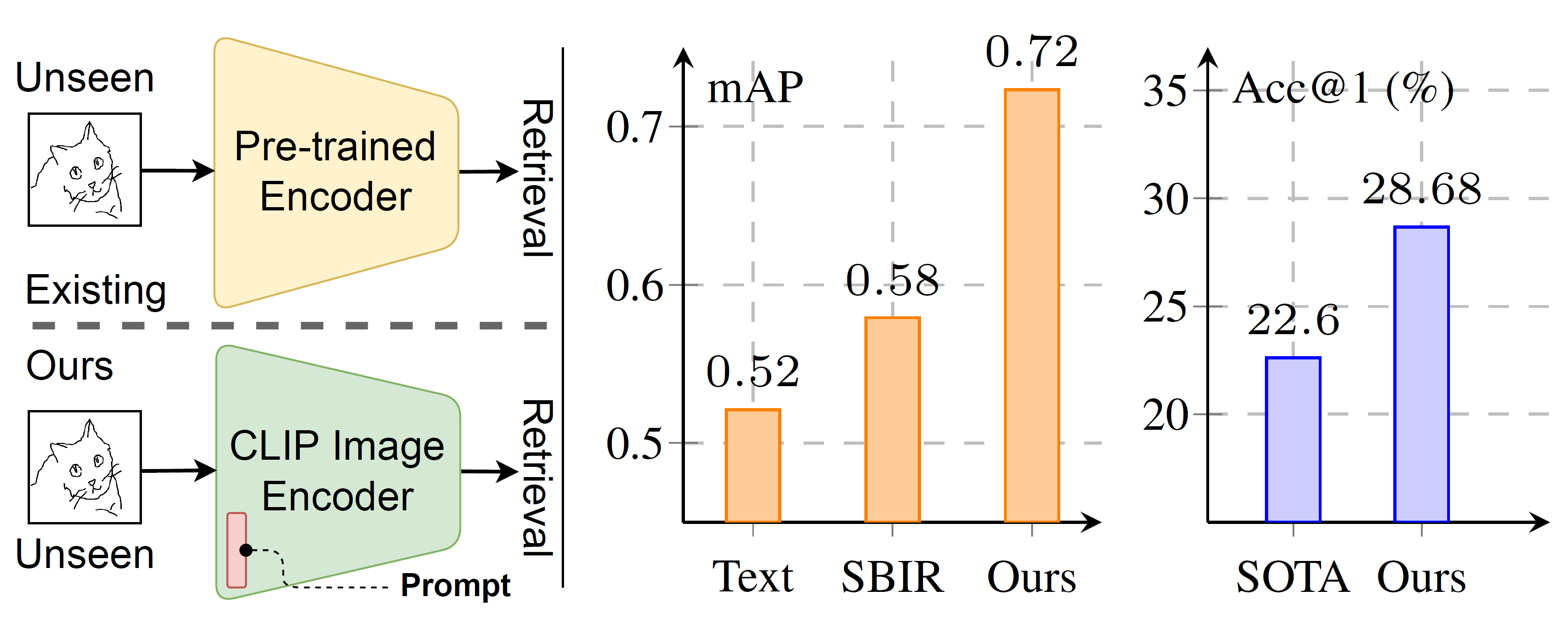
Figure 1: Against existing (left) ZS-SBIR methods, we adapt CLIP model for ZS-SBIR (middle), and extend to a more practical yet challenging setup of FG-ZS-SBIR (right), via a novel prompt-based design. Our model surpasses prior arts by a high margin.

At the very heart of our answer to this synergy is that of prompt learning [29], that involves learning a set of continuous vectors injected into CLIP’s encoder. This enables CLIP to adapt to downstream tasks while preserving its generalisability – a theme that we follow in our CLIP-adaption to ZS-SBIR (Fig. 1). More specifically, we first design two sets of visual prompts, one for each modality (sketch, photo). They are both injected into the initial layer insider the transformer of CLIP for training. While keeping the rest of CLIP frozen, these two prompts are trained over the gold standard triplet loss paradigm [70], on extracted sketch-photo features. Motivated by the efficacy of training batch normalisation for image recognition [21], we additionally fine-tune a small subset of trainable parameters of every Layer Normalisation (LN) layer for additional performance gain. Furthermore, to enhance cross-category semantic transfer, we also resort to CLIP’s text encoder further cultivating its zero-shot potential. In particular, in addition to the said visual prompts onto the CLIP’s image encoder, we use handcrafted text prompts via templates like ‘photo of a [category]’ to its text encoder, during training.

The new fine-grained setting [44, 13] is however more tricky. Unlike the previous category-level setup, it poses two additional challenges (i) relative feature-distances between sketch-photo pairs across categories are non-uniform, which is reflected in the varying triplet-loss margin [70] across categories at training [8], and (ii) apart from semantic consistency, fine-grained ZS-SBIR requires instance-level matching to be conducted [44], which dictates additional constraints such as structural correspondences.

It follows that for the first challenge, we propose a new regularisation term that aims at making the relative sketch-photo feature-distances uniform across categories, such that a single (global) margin parameter works across all of them. Specifically, taking the distribution of relative distances for all sketch-positive-negative hard-triplets [70] in a category, we aim to minimise the KL-divergence [40] between every pair of distributions, which trains the model towards making such relative sketch-photo distances uniform across categories. For the latter, we propose a clever patch shuffling technique, where equally divided patches of a sketch and its corresponding photo (n$\times$n) are first shuffled following a random permutation order of patches. We then advocate that a shuffled sketch should be closer to a shuffled photo having the same permutation order, but far from that of a different permutation. Training this permutation-invariance imparts a broad notion of structural correspondences, thus helping in fine-grained understanding.

Summing up: (i) We for the first time adapt CLIP for ZS-SBIR, (ii) We propose a novel prompt learning setup to facilitate the synergy between the two, (iii) We address both the conventional ZS-SBIR setting, and a new and more challenging fine-grained ZS-SBIR problem, (iv) We introduce a regularisation term and a clever patch shuffling technique to address the fine-grained challenges. With our CLIP-adapted model surpassing all prior arts by a large margin (Fig. 1), we hope to have shed some light to the sketch community on benefits such a synergy between foundation models and sketch-related tasks can bring.

2 Related Work

Category-level SBIR:  Given a query-sketch, SBIR aims at fetching category-specific photos from a gallery of multi-category photos. Recent deep-frameworks aim to learn a joint sketch-photo manifold via a feature extractor  [14, 16, 68, 68] over a triplet-ranking objective [70]. Towards practicality of unseen test-time classes, Zero-Shot SBIR (ZS-SBIR) was explored for cross-category generalisation [16, 69], and enhanced via test-time training [50]. Others explored binary hash-codes [35, 73] for computational ease. Sketch however specializing in modelling fine-grained details, geared research towards Fine-Grained SBIR.

Fine-grained SBIR:  FG-SBIR aims at retrieving one instance from a gallery of same-category images based on a query-sketch. Introduced as a deep triplet-ranking based siamese network [70] for learning a joint sketch-photo manifold, FG-SBIR was improvised via attention-based modules with a higher order retrieval loss [60], textual tags [59, 12], hybrid cross-domain generation [43], hierarchical co-attention [51] and reinforcement learning [9]. Furthermore, sketch-traits like style-diversity [52], data-scarcity [5] and redundancy of sketch-strokes [6] were addressed in favor of retrieval. Towards generalising to novel classes, while [42] modelled a universal manifold of prototypical visual sketch traits embedding sketch and photo, [8] adapted to new classes via some supporting sketch-photo pairs. In this paper, we aim to address the problem of zero-shot cross-category FG-SBIR, leveraging the zero-shot potential of a foundation model like CLIP [46].

Zero-Shot SBIR:  This aims at generalising knowledge learned from seen training classes to unseen testing categories. Yelamarthi et al. [69] introduced ZS-SBIR, to reduce sketch-photo domain gap by approximating photo features from sketches via image-to-image translation. While, [18] aligned sketch, photo and semantic representations via adversarial training, [16] minimised sketch-photo domain gap over a gradient reversal layer. Improvising further, others used graph convolution networks [74], or distilled contrastive relationships [63] in a student from ImageNet-pretrained teacher, coupled skecth/photo encoders with shared conv layers and independent batchnorm-layer [65], a shared ViT [62] to minimise domain gap, or employed prototype-based selective knowledge distillation [66] on learned correlation matrix, and very recently introduced a test-time training paradigm [50] via reconstruction on test-set sketches, adapting to the test set distribution. Semantic transfer for ZS-SBIR however was mostly limited to using word embeddings directly [18, 74, 65] or indirectly [63, 37, 66]. Furthermore, FG-ZS-SBIR being non-trivial remains to be explored. In this paper, we thus take to adapting CLIP to exploit its high generalisability for semantic transfer and exploring its zero-shot potential for FG-ZS-SBIR.

CLIP in Vision Tasks:  Contrastive Language-Image Pre-training (CLIP) [46] trains on cross-modal data, benefiting both from rich semantic textual information [47] and large scale availability of images ($\sim 400$M image-text pairs) for training. Unlike traditional representations on discretized labels, CLIP represents images and text in the same embedding space [47], thus enabling generalizability in downstream tasks with no labels (zero-shot) [75] or a few annotations (few-shot) [76] by generating classification weights from text encodings. Efficiently adapting CLIP for downstream tasks to exploit it’s zero shot potential has been investigated using Prompt engineering from NLP literature [36]. Such common extensions include retrieval [4], image generation [11], continual learning [61], object detection, few-shot recognition [22], semantic segmentation [47], etc. Others leveraged CLIP’s image/text encoders with StyleGAN [45] to enable intuitive text-based semantic image manipulation [1]. In our work we adapt CLIP for zero-shot FG-SBIR in a cross-category setting.

Prompt Learning for Vision Tasks:  Originating from NLP domain, prompting [10] imparts context to the model regarding the task at hand, thus utilising the knowledge base of large-scale pretrained text models like GPT and BERT to benefit downstream tasks. This involves constructing a task specific template (e.g., ‘The movie was [MASK]’), and label words (e.g. ‘good/bad’) to fill it up. Domain-expertise being necessary for hand-crafted prompt-engineering, urged the need for prompt tuning in recent works [29], which entails modelling the prompt as task-specific learnable continuous vectors that are directly optimised via gradient descent during fine-tuning. Learning context vectors for prompting has also taken root in the vision community [3], with greater emphasis on prompting large scale vision language models [75] or visual feature extractors (e.g. ViT [29]). Unlike previous attempts at prompt learning [76, 29], in context of FG-SBIR, we focus on learning a single prompt for sketch and photo branches which when used with CLIP, would generalise on to unseen novel classes by leveraging the zero-shot potential of CLIP for multi-category FG-ZS-SBIR.

3 Preliminaries

Overview of CLIP:  Contrastive Language-Image Pre-training or CLIP [46], widely popular for open-set visual understanding tasks, consists of two separate encoders, one for image and another one for text. The image encoder ($\mathbf{V}$) uses either ResNet-50 [26] or a Vision Transformer (ViT) [17], where an input image ($p\in\mathbb{R}^{H\times W\times 3}$) is divided into $m$ fixed-size patches and embedded as $E_{0}$ = $\{\mathbf{e}_{0}^{j}\}_{j=1}^{m};\mathbf{e}_{0}^{j}\in\mathbb{R}^{d_{p}}$. Similar to BERT’s [CLASS] token, a learnable class token $c_{0}^{t}\in\mathbb{R}^{d}_{p}$ is appended, and the resultant matrix $[E_{0},c_{0}^{v}]\in\mathbb{R}^{(m+1)\times d}$ is passed through transformer layers, followed by a feature projection layer on class-token feature to obtain the final visual feature $f_{p}=\mathbf{V}(p)\in\mathbb{R}^{d}$ in joint vision-language embedding space. Similarly, using a vocab-size of $49,152$, the text encoder $\mathbf{T}$ first converts a sentence with $n$ words (including punctuation) to word embeddings as $W_{0}$ = $\{\mathbf{w}_{0}^{j}\}_{j=1}^{n}\;;\mathbf{w}_{0}^{j}\in\mathbb{R}^{d_{t}}$ and appends a learnable class token $c_{0}^{t}\in\mathbb{R}^{d_{t}}$ to form the input feature matrix $[W_{0},c_{0}^{t}]\in\mathbb{R}^{(n+1)\times d_{t}}$ representing knowledge of the sentence ($\mathcal{S}$), which is passed via a transformer to extract textual feature $f_{t}=\mathbf{T}(\mathcal{S})$. The model is trained via a contrastive loss [46] maximising cosine similarity for matched text-photo pairs while minimising it for all other unmatched pairs. During downstream tasks like classification [46], textual prompts like ‘a photo of a [category]’ (from a list of $K$ categories) are fed to $\mathbf{T}$ to obtain category-specific text features ($f_{t}$) and calculate the prediction probability for input photo feature ($f_{p}$) as:

$$\mathcal{P}(y|p)=\frac{\mathrm{exp}(\texttt{sim}(f_{p},f_{t}^{y})/\tau)}{\sum_{i=1}^{K}\mathrm{exp}(\texttt{sim}(f_{p},f_{t}^{i})/\tau)}\vspace{-0.15cm}$$ (1)

Prompt Learning:  Following NLP literature [10], prompt learning has been adopted on foundation models like CLIP [75] or large-pretrained Vision Transformers [29] to benefit downstream tasks. Unlike previous fine-tuning based methods [44] that entirely updated weights of pre-trained models on downstream task datasets, prompt learning keeps weights of foundation models frozen to avoid deploying separate copy of large models for individual tasks besides preserving pre-learned generalizable knowledge. For a visual transformer backbone, concatenated patch-features and class tokens ($[E_{0},c_{0}^{v}]\in\mathbb{R}^{(m+1)\times d_{p}}$), appended with a set of $K$ learnable prompt vectors $\mathbf{v}^{p}$ = $\{v_{i}\}_{i=1}^{K};v_{i}\in\mathbb{R}^{d_{p}}$ for photo $p$, as $[E_{0},c_{0}^{v},\mathbf{v}^{p}]$ $\in\mathbb{R}^{(m+1+K)\times d_{p}}$, and passed via the transformer to obtain $\widehat{f_{p}}$ = $\mathbf{V}(p,\mathbf{v}^{p})$. Keeping the entire model fixed, $\mathbf{v}^{p}$ is fine-tuned on the task-specific dataset, adapting the foundation model to the task at hand. Variations of prompt learning include, shallow vs deep prompt [29], based on the layers at which prompts are inserted. Here, we use simple shallow prompt that is inserted only at the first layer along-with patch embeddings, which empirically remains optimal and easy to reproduce.

4 CLIP for Zero-Shot Category-level SBIR

Baseline Categorical SBIR:  Given a query-sketch ($s$) from any category, categorical SBIR [50] aims to retrieve a photo of the same category, from a gallery ($\mathcal{G}$) holding photos from multiple ($N_{c}$) categories $\mathcal{G}$ = $\{p^{j}_{i}\}_{i=1}^{M_{i}}|_{j=1}^{N_{c}}$, where $i^{\text{th}}$ class has $M_{i}$ number of photos. Formally, an embedding (separate for sketch and photo) function $\mathcal{F}(\cdot):\mathbb{R}^{H\times W\times 3}\rightarrow\mathbb{R}^{d}$, usually represented by an ImageNet[33]-pretrained VGG-16 [58], is trained to extract a $d$-dimensional feature from an input image (sketch $s$ /photo $p$) $\mathcal{I}$ as $f_{\mathcal{I}}=\mathcal{F}_{\mathcal{I}}(\mathcal{I})\in\mathbb{R}^{d}$, over a triplet loss [70] using the feature triplet of a query-sketch ($f_{s}$) and a photo ($f_{p}$) belonging to the same category, and another photo from a different category ($f_{n}$). Minimising the triplet loss ($\mathcal{L}_{\text{Tri}}$) signifies bringing sketches and photos of the same category closer while distancing other categories’ photos. With $\mu$ as margin and distance function $d(a,b)$ = $({1-a\cdot b})/({||a||-||b||})$, triplet loss is given as,

$$\mathcal{L}_{\text{Tri}}=\max\{0,\mu+d(f_{s},f_{p})-d(f_{s},f_{n})\}$$ (2)

Unlike normal SBIR, evaluating on categories seen during training $\mathcal{C}^{\text{S}}$ = $\{c^{\text{S}}_{i}\}^{N_{\text{S}}}_{i=1}$, ZS-SBIR [16] evaluates on novel ones $\mathcal{C}^{\text{U}}$ = $\{c^{\text{U}}_{i}\}^{N_{\text{U}}}_{i=1}$, unseen during training, i.e, $\mathcal{C}^{\text{S}}\cap\mathcal{C}^{\text{U}}=\emptyset$.

Naively Adapting CLIP for ZS-SBIR:  Although the SBIR baseline can be naively extended to a zero-shot setting for ZS-SBIR [16], it performs unsatisfactorily lacking sufficient zero-shot transfer [61, 39] of semantic knowledge. Consequently, a very naive extension upon CLIP would be to replace ImageNet[48]-pretrained VGG-16 by the CLIP’s visual encoder, which already holds semantic-rich information, thus directly harnessing its inherent zero-shot potential for ZS-SBIR. Following traditional fine-tuning methods [44], if we start naively training the CLIP’s image encoder on SBIR dataset using triplet loss, the performance collapses due to catastrophic forgetting [50] of learnt CLIP knowledge. Alternatively, focusing on parameter-efficient paradigm, one may train via an additional MLP layer at the end [22], while keeping the remaining network frozen. As this essentially transfers the encoded feature from CLIP’s embedding space to a subsequent space via the MLP layer, it does not guarantee CLIP’s generalisation potential to remain preserved [29], thus defeating our sole purpose of adapting CLIP for ZS-SBIR. Avoiding such loopholes, we therefore opt for a prompt learning approach [75] that not only provides stable optimisation [31] but also preserves the desired generalisation (open-vocab) [76] of CLIP.

Prompt Learning for ZS-SBIR:  To adapt CLIP for category-level SBIR, we learn two sets of sketch/photo visual prompts as $\mathbf{v}^{s},\mathbf{v}^{p}\in\mathbb{R}^{K\times d_{p}}$, each of which is injected into respective sketch $\mathcal{F}_{s}$ and photo $\mathcal{F}_{p}$ encoders both initialised from CLIP’s image encoder, respectively. Finally, we get the prompt guided sketch feature $f_{s}$ = $\mathcal{F}_{s}(s,\mathbf{v}^{s})\in\mathbb{R}^{d}$ and photo feature $f_{p}$ = $\mathcal{F}_{p}(p,\mathbf{v}^{p})\in\mathbb{R}^{d}$, respectively. In essence, the sketch and photo specific prompts induce CLIP [46] to learn the downstream sketch and photo distribution respectively. Knowledge learned by CLIP is distilled into a prompt’s weights via backpropagation keeping CLIP visual encoder’s weights ($\theta$) frozen. While freezing $\theta$ is motivated by training stability [76, 75], we take a step further and ask, can we improve CLIP by fine-tuning $\theta$ yet enjoy training stability? Accordingly, instead of fine-tuning $\theta$ entirely, we tune a small subset – the trainable parameters of every layer normalisation (LN) layers across $\theta$. Our design is motivated by prior observation [21] on unusual efficacy of training batch normalisation for image recognition, keeping rest of parameters frozen. Therefore, besides the prompt parameters $\{\mathbf{v}^{s},\mathbf{v}^{p}\}$, we update the parameters of sketch/photo branch specific layer-norm layers’s parameters $\{l_{\theta}^{s},l_{\theta}^{p}\}$ via standard triplet loss as in Eq. 2. The trainable parameter set is $\{\mathbf{v}^{s},\mathbf{v}^{p},l_{\theta}^{s},l_{\theta}^{p}\}$.

Classification Loss using CLIP’s Text Encoder:  Besides using CLIP’s image encoder for zero-shot utility, we further exploit the high generalisation ability provided by natural language [15, 46] through CLIP’s text encoder. In particular, along with the triplet loss, we impose a classification loss on the sketch/photo joint-embedding space. For this, instead of usual auxiliary $N_{s}$-class FC-layer based classification head [8, 19, 16], we take help of CLIP’s text encoder to compute the classification objective, which is already enriched with semantic-visual association. Following [24], we construct a set of handcrafted prompt templates like ‘a photo of a [category]’ to obtain a list classification weight vectors $\{t_{j}\}_{j=1}^{N_{s}}$ using CLIP’s text encoder where the ‘[category]’ token is filled with a specific class name from a list of $N_{s}$ seen classes. The classification loss for $\mathcal{I}=\{s,p\}$ is given by:

$$\mathcal{L}^{\mathcal{I}}_{\text{cls}} =\frac{1}{N}\sum_{i=1}^{N}-\log\mathcal{P}(y_{i}|I_{i})\quad\text{where,}$$ (3)

$$\mathcal{P}(y_{i}|I_{i}) =\frac{\text{exp}(\texttt{sim}(\mathcal{F}_{\mathcal{I}}(\mathcal{I}_{i}),t_{y})/\tau)}{\sum^{N_{s}}_{j=1}\text{exp}(\texttt{sim}(\mathcal{F}_{\mathcal{I}_{i}}(\mathcal{I}),t_{j})/\tau)}$$

Summing up our CLIP adapted ZS-SBIR paradigm is trained using a weighted ($\lambda_{1}$) combination of losses as : $\mathcal{L}^{\text{ZS-SBIR}}_{\text{Trn}}=\mathcal{L}_{\text{Tri}}+\lambda_{1}(\mathcal{L}^{p}_{\text{cls}}+\mathcal{L}^{s}_{\text{cls}})$.

While off-the-shelf CLIP itself has zero-shot image retrieval potential [30, 61] where someone can feed the category level query as ‘a photo of a [query]’, it raises a question – how much is a category-level query-sketch beneficial over text-keyword based query? Attending to sketch’s specialty in modelling fine-grained [51, 70, 6] details hence, we go beyond category-level ZS-SBIR [16, 18] to a more practical and long-standing research problem of cross-category fine-grained ZS-SBIR [44].

5 CLIP for Zero-Shot Fine-grained SBIR

Background on FG-SBIR:  Compared to category-level SBIR [50], fine-grained SBIR [70] aims at instance-level sketch-photo matching at intra-category level. Most of existing FG-SBIR works remain restricted to single-category setup, where they train and evaluate on the same category, like the standard FG-SBIR dataset (e.g., QMUL-ShoeV2 [70]), that comprises $k$ instance-level sketch/photo pairs as $\{s_{i},p_{i}\}_{i=1}^{k}$. A baseline FG-SBIR framework [70] involves training a backbone network, shared between sketch and photo branches using a triplet-loss based objective [70] where the matched sketch-photo pairs respectively form the anchor ($s_{i}$) and positive ($p_{i}$) samples, whereas a random photo $(p_{\neq i})$ is considered as the negative.

A few works have extended it to multi-category FG-SBIR [8] setup which aims to train a single model with instance-level matching from multiple ($N_{c}$) categories (e.g., Sketchy dataset [53]). The dataset consists of sketch/photo pairs from multiple categories $\{s_{i}^{j},p_{i}^{j}\}_{i=1}^{k_{j}}|_{j=1}^{N_{c}}$ with every $j^{\text{th}}$ class having $k_{j}$ sketch-photo pairs. On top of baseline for single-category FG-SBIR [51], it involves two additional design considerations (i) Hard-triplets for triplet loss based training where the negative photo $(p_{\neq i}^{j})$ is from the same $j^{\text{th}}$ class of sketch-anchor ($s_{i}^{j}$) and positive-photo ($p_{i}^{j}$), but of different instances ($\mathcal{L}^{\text{hard}}_{\text{Tri}}$), (ii) an auxiliary $N_{c}$-class classification head on the sketch/photo joint embedding space to learn the class discriminative knowledge.

Moving on, cross-category zero-shot FG-SBIR [42] is analogous to category-level ZS-SBIR, in that the training and testing categories are disjoint ($\mathcal{C}^{\text{S}}\cap\mathcal{C}^{\text{U}}=\emptyset$), but the former needs to fetch instance-level photos from unseen categories instead of merely retrieving at category level like the latter. We therefore aim to answer the question: how can we extend our CLIP-based ZS-SBIR to FG-ZS-SBIR?

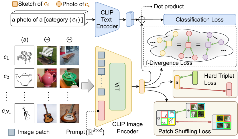
Figure 2: Cross-category FG-ZS-SBIR. A common (photo-sketch) learnable visual prompt shared across categories is trained using CLIP’s image encoder over three losses as shown. CLIP’s text-encoder based classification loss is used during training.

Extending CLIP-based ZS-SBIR to FG-ZS-SBIR:  To recap (Fig. 2), the key components of CLIP-based ZS-SBIR are: (i) CLIP image-encoder as backbone with separate sketch/photo branches with individual prompts $\{\mathbf{v}^{s},\mathbf{v}^{p}\}$, (ii) category-level triplets (iii) CLIP text-encoder [46] based classification loss, and (iv) fine tuning layer-norms for sketch/photo branches. Keeping rest of the design same, the necessary modification for intra-category instance-level matching (FG-ZS-SBIR) is to replace the category-level triplets by hard-triplets – ($s_{i}^{j},p_{i}^{j},p_{\neq i}^{j}$) all from the same category but different negative instances. Furthermore, we empirically found that a common prompt [29] and a shared backbone [70] between sketch/photo branches works better for fine-grained matching. The only trainable parameter set is thus a common prompt $\mathbf{v}$ and layer-norm parameters $l_{\theta}$.

However, there are two major bottlenecks: Firstly, due to instance level matching across categories, the category-specific margin-parameter of triplet loss ($\mu$) varies significantly [8], showing that a single global margin-value alone is sub-optimal for training a FG-ZS-SBIR model. Secondly, due to the diverse shape morphology [52] amongst varying categories, it becomes extremely challenging to recognise fine-grained associations for unseen classes whose shape is unknown. We therefore need a training signal to explicitly learn the structural correspondences in a sketch-photo pair.

Stabilising Margin ($\mu$) across Categories:  Recently a work [8] on multi-category FG-SBIR has empirically shown optimal margin ($\mu$) value to vary across different categories. Looking closely at triplet loss, $\mathcal{L}=\max(0,\mu+d(s,p^{+})-d(s,p^{-}))$ [71], it essentially computes the difference between positive ($(s,p^{+})$) and negative distances ($(s,p^{-})$). We term this difference as the relative distance $\delta(s,p^{+},p^{-})=d(s,p^{+})-d(s,p^{-})$. Using a constant $\mu$ means that on average, the relative distance is same for any triplet $(s,p^{+},p^{-})$ [60] in a category. Contrarily, a varying $\mu$ across different categories signifies that the average relative distance across categories is not uniform [8]. Therefore, naively training with a single $\mu$ value across all seen categories would be sub-optimal, and affect the cross-category generalisation of triplet loss [44] which importantly works on this relative distance. While [8] tackles this issue by meta-learning [27] the margin value using few-shot sketch/photo pairs, ours is entirely a zero-shot setup [16], rendering such adaptation infeasible. We thus impose a regulariser that aims to make this relative distance uniform across categories such that the same triplet loss, with single (global) margin parameter $\mu$ works for all categories. To achieve this, we first compute the distribution of relative distances [38, 23] for all triplets $(s,p^{+},p^{-})$ in category $c$ as $\mathcal{D}_{c}=\mathrm{softmax}\{\delta(s_{i},p^{+}_{i},p^{-})\}_{i=1}^{N_{s}}$, where $c^{th}$ category has $N_{s}$ sketch-photo pairs. Next, towards making the relative distance uniform across categories, we minimise the KL-divergence [40] between a distribution of relative distances between every category-pair (aka. f-divergence [23]) as:

$$\mathcal{L}_{\delta}=\frac{1}{N_{s}(N_{s}-1)}\sum_{i=1}^{N_{s}}\sum_{j=1}^{N_{s}}\texttt{KL}(\mathcal{D}_{i},\mathcal{D}_{j})\vspace{-0.2cm}$$ (4)

In practice, we compute $\mathcal{L}_{\delta}$ using sketch/photo samples from every category appearing in a batch. Importantly the spread, or relative entropy [56] or information radius [57] of distribution $\delta$ should be similar, thus stabilising training with a single margin value for multi-category FG-ZS-SBIR.

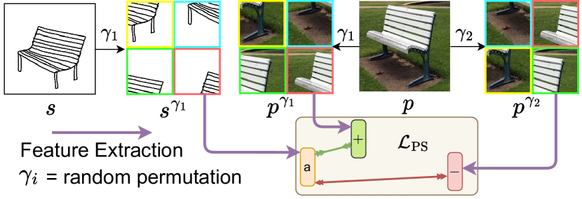
Figure 3: Patch-shuffling for fine-grained transfer

.

Patch-shuffling for Zero-Shot Fine-grained Transfer:  Category-level SBIR is subtly different from FG-SBIR [70] in that the former focuses only on semantic similarity between sketch-photo pairs, unlike FG-SBIR that takes a step further to focus on fine-grained shape matching [8] between sketches and photos. Highly diverse shape morphology [52] across new categories implies unconstrained domain gap for multi-category FG-SBIR, thus increasing its difficulty. Discovering fine-grained correspondence becomes even harder as shape itself becomes unknown for unseen categories [8].

For better fine-grained shape-matching transfer to novel classes, we design a simple data-augmentation trick through patch-shuffling to create augmented triplets [60]. In particular, we permute $\mathbf{n}\times\mathbf{n}$ patches (numbered) of sketch ($s$) and photo ($p$) using $\psi(\cdot)$ as $s^{\gamma}$ = $\psi(s,\gamma)$ and $p^{\gamma}$ = $\psi(p,\gamma)$, where $\gamma$ denotes a random permutation of the array $[1,2,...\mathbf{n}^{2}]$ describing the mapping of image patches to $s^{\gamma}$ or $p^{\gamma}$ (LABEL:{fig:patch_shuffle}). Given a sketch-photo pair of any category ($s,p$), training should decrease feature-distance of the sketch-permutation ($s^{\gamma_{1}}$) from the same permutation ($\gamma_{1}$) of its paired photo ($p^{\gamma_{1}}$), while increasing it from a different permutation ($p^{\gamma_{2}}$). Accordingly, we devise a triplet [70] training objective as :

$$\mathcal{L}_{\text{PS}}=\max\{0,\mu_{ps}+d(f_{s^{\gamma_{1}}},f_{p^{\gamma_{1}}})-d(f_{s^{\gamma_{1}}},f_{p^{\gamma_{2}}})\}\vspace{-0.15cm}$$ (5)

In contrast to auxiliary patch-order prediction, we found that our triplet objective between similar and dissimilar permuted instances provides better fine-grained shape transfer, besides being much cheaper during trainsing compared to complex Sinkorn operation [2] as used by Pang et al. [44].

With $\lambda_{2,3,4}$ as hyperparameters, our overall training objective for CLIP adapted FG-ZS-SBIR paradigm is given as, $\mathcal{L}^{\text{FG-ZS-SBIR}}_{\text{Trn}}=\mathcal{L}_{\text{Tri}}^{\text{hard}}+\lambda_{2}(\mathcal{L}_{\text{cls}}^{s}+\mathcal{L}_{\text{cls}}^{p})+\lambda_{3}\mathcal{L}_{\delta}+\lambda_{4}\mathcal{L}_{\text{PS}}$.

6 Experiments

Datasets:  We use three popular datasets for evaluation on ZS-SBIR. (i) Sketchy (extended) [35] – Sketchy [53] contains 75,471 sketches over 125 categories having 100 images each [69]. We use its extended version [35] having extra 60,502 images from ImageNet [48]. Following [69] we split it as 104 classes for training and 21 for testing for zero-shot setup. (ii) TUBerlin [20] – contains 250 categories, with 80 free-hand sketches in each, extended to a total of 204,489 images by [72]. Following [16] We split it as 30 classes for testing and 220 for training. (iii) QuickDraw Extended [25]– The full-version houses over 50 million sketches across 345 categories. Augmenting them with images, a subset with 110 categories having 330,000 sketches and 204,000 photos was introduced for ZS-SBIR [16], which we use, following their split of 80 classes for training and 30 for testing. Requiring fine-grained sketch-photo association [60] for evaluating cross-category FG-ZS-SBIR, we resort to Sketchy [53] with fine-grained sketch-photo association, using the same zero-shot categorical split of 104 training and 21 testing classes [69].

Implementation Details:  We implemented our method in PyTorch on a 11GB Nvidia RTX 2080-Ti GPU. For sketch/photo encoder, we use CLIP [46] with ViT backbone using ViT-B/32 weights. For both paradigms of ZS-SBIR and FG-ZS-SBIR the input image size is set as $224\times 224$ with margin parameter $\mu$=$0.3$, and prompts are trained using Adam optimiser with learning rate $1e-5$ for $60$ epochs, and batch size $64$, while keeping CLIP model fixed except its LayerNorm layers. We use two prompts (sketch and photo) from ZS-SBIR and one common prompt for FG-ZS-SBIR, each having a dimension of $(3\times 768)$. Our prompts are injected in the first layer of transformer. For FG-ZS-SBIR $\mathbf{n}$=2 patches are used for patch shuffling-objective. Values of $\lambda_{1,2,3,4}$ are set to $0.5$, $0.5$, $0.1$ and $1$, empirically.

Evaluation Metric:  Following recent ZS-SBIR literature [16, 28, 66] we perform ZS-SBIR evaluation considering the top 200 retrieved samples, reporting mAP score (mAP@all) and precision (P@200) for ZS-SBIR. Keeping consistency with recent ZS-SBIR works however, we report P@100 and map@200 specifically for TUBerlin [72] and Sketchy-ext [35] respectively. For cross-category FG-ZS-SBIR, accuracy is measured taking only a single category at a time [44], as Acc.@q [70] for Sketchy [53], which reflects percentage of sketches having true matched photo in the top-q list. We use Top-1 and Top-5 lists [8].

Table 1: Quantitave comparison of our method against existing frameworks and baselines on ZS-SBIR and cross-category FG-ZS-SBIR.

Zero-Shot SBIR									Cross-category Zero-Shot FG-SBIR
Methods			Sketchy		TU-Berlin		QuickDraw		Methods	Sketchy
			mAP@200	P@200	mAP@all	P@100	mAP@all	P@200		Top-1	Top-5
ZS-SOTA	ECCV ’18	ZS-CAAE [69]	0.156	0.260	0.005	0.003	–	–
	ECCV ’18	ZS-CVAE [69]	0.225	0.333	0.005	0.001	0.003	0.003	Cross-GRAD [55]	13.4	34.90
	CVPR ’19	ZS-CCGAN [18]	–	–	0.297	0.426	–	–
	CVPR ’19	ZS-GRL [16]	0.369	0.370	0.110	0.121	0.075	0.068	CC-DG [42]	22.6	49.00
	ICCV’19	ZS-SAKE [37]	0.497	0.598	0.475	0.599	–	–
	AAAI ’20	ZS-GCN [74]	0.568	0.487	0.110	0.121	–	–	B-FG-FT	1.23	4.56
	NeurIPS ’20	ZS-IIAE [28]	0.373	0.485	0.412	0.503	–	–
	TPAMI ’21	ZS-TCN [65]	0.516	0.608	0.495	0.616	0.140	0.298	B-FG-Lin	15.75	39.63
	AAAI ’22	ZS-TVT [62]	0.531	0.618	0.484	0.662	0.149	0.293
	ACM MM ’22	ZS-PSKD[ViT] [66]	0.560	0.645	0.502	0.662	0.150	0.298	B-FG-Cond	25.98	54.38
	CVPR ’22	ZS-Sketch3T [50]	0.579	0.648	0.507	0.671	–	–
B-CLIP		B-FT	0.102	0.166	0.003	0.001	0.001	0.001	B-FG-IP	26.69	56.08
		B-Lin	0.422	0.512	0.398	0.557	0.082	0.098
		B-Cond	0.618	0.675	0.562	0.648	0.159	0.312	B-FG-MM	27.16	59.46
		B-IP	0.691	0.711	0.628	0.702	0.182	0.361
		B-MM	0.685	0.691	0.604	0.678	0.171	0.347	B-FG-Deep	27.62	61.56
		B-Deep	0.702	0.718	0.637	0.718	0.188	0.375
		Ours	0.723	0.725	0.651	0.732	0.202	0.388	Ours	28.68	62.34

6.1 Competitors

First we compare against State-of-the-arts for ZS-SBIR and FG-ZS-SBIR. For ZS-SBIR (ZS-SOTA), while ZS-CVAE [69] and ZS-CAAE [69] employs sketch-to-image translation, ZS-CCGAN [18] and ZS-GRL [16] both use word2vec[41] embeddings for semantic transfer, with adversarial learning and gradient-reversal layer respectively. Apart from using knowledge-distillation (KD) (ZS-SAKE) [37], or learning a correlation matrix via prototype-based selective KD (ZS-PSKD [37]), complex designs like graph convolution network (ZS-GCN), coupled sketch/photo encoder (ZS-TCN [65]) with shared conv layers but independent batchnorm layer, or complicated three-way ViT [17] architecture (ZS-TVT [62]) for visual/semantic transfer have been used. While ZS-IIAE [28] enforces cross-domain disentanglement, ZS-Sketch3T[50] uses a test-time training paradigm to minimise the train-test distribution gap. For FG-ZS-SBIR, we compare against CrossGrad [55] that leverages hard triplets with a category/domain classifier using word2vec embedded class-labels, and CC-DG [42] that models a universal manifold of prototypical visual sketch traits towards generalising to unseen categories. We report their results directly from their papers.

Next we design a few baselines (B) for adapting CLIP to ZS-SBIR and ZS-FG-SBIR paradigms. For all of them, the prompt design remains same for both paradigms, but every baseline of ZS-SBIR (B-) is extended to FG-ZS-SBIR (B-FG-) across multiple categories using hard-triplets and a CLIP text-encoder based classification loss. B-FT and B-FG-FT fine-tune a pre-trained ViT-B/16 CLIP-Image Encoder [46], for ZS-SBIR with a low learning rate of 1e-6. Similarly, B-Lin and B-FG-Lin use a linear probe [46] to train an additional feature embedding layer on top of pre-trained CLIP features to adapt to ZS-SBIR and FG-ZS-SBIR respectively, keeping image-extractor backbone frozen. Following [75], B-Cond and B-FG-Cond, learns to generate a sketch-conditioned (for every sketch) prompt via a lightweight network (ResNet-18), when after concatenation with image-patch features are fed to the CLIP’s image encoder. B-IP and B-FG-IP learn two independent shallow prompts, for sketch and photo, that are injected in the first ViT [17] layer following [76] for ZS-SBIR and FG-ZS-SBIR respectively. Instead of independent sketch and photo prompts B-MM and B-FG-MM adapts [30] to learn a multi-modal prompt for both sketch and photo to ensure mutual synergy and discourage learning independent uni-modal solutions. More specifically, we learn a single photo prompt from which the sketch prompt is obtained as a photo-to-sketch projection, via a linear layer. B-Deep and B-FG-Deep employ deep prompting [29] learning $N=9$ prompts for sketch and photo, injected into the first $N$ layers of ViT [17] backbone. The last three types for both paradigms importantly differ from our method in keeping their LayerNorm frozen, which we fine-tune for better accuracy.

6.2 Performance Analysis:

ZS-SBIR:  While state-of-the-arts offer reasonable performance (Table 1) thanks to their respective strategies of semantic transfer via word2vec (ZS-GRL), adaptation via test-time training (ZS-Sketch3T) or improvised transformer-based (ZS-TVT), distillation-based (ZS-PSKD) and other setups, our method armed with open-vocab generalisable potential of CLIP, surpasses them in all three datasets. Although naively adapting large foundation models like CLIP [46] (e.g., B-FT) understandably collapses, a successful adaptation outperforms existing SOTAs by $\approx 24.8\%$ (avg). This motivates CLIP [47] as the default sketch/photo encoders for future sketch research. While linear probing in B-Lin secures higher results than SOTAs, it is surpassed by prompt-based learning, thus providing insights on a better adaptation choice. The marginal difference in performance between a simple adaptation of CLIP in B-IP and more its complicated versions in B-Deep [29], B-MM, B-Cond, motivates the use of a simple shallow prompt without the added “bells and whistles” for ZS-SBIR. Finally, high accuracy on ZS-SBIR, establishes CLIP as a robust choice for sketch-based systems and thus motivates consequent focus on the more challenging task of cross-category FG-ZS-SBIR.

Cross-category FG-ZS-SBIR:  Our CLIP adapted paradigm easily surpasses the two existing SOTAs on cross-category FG-ZS-SBIR (Table 1 right). While CLIP models [47] shows impressive performance at category-level ZS-SBIR, there is reasonable scope for improvement in FG-ZS-SBIR that additionally requires structural matching[44]. Relatively higher improvement of B-FG-MM over B-FG-IP [76] than its category-level counterpart (B-MM over B-IP), suggests the efficacy of multi-modal prompts over independent sketch/photo prompts, in FG-SBIR. This supports the prior observation [70] that sharing encoder parameters is more suited to FG-SBIR [51] whereas separate sketch/photo weights work best at category-level. Lastly, learning a conditional prompt [75] in B-FG-Cond offers marginal gain due to its sensitivity to training strategies [30, 75].

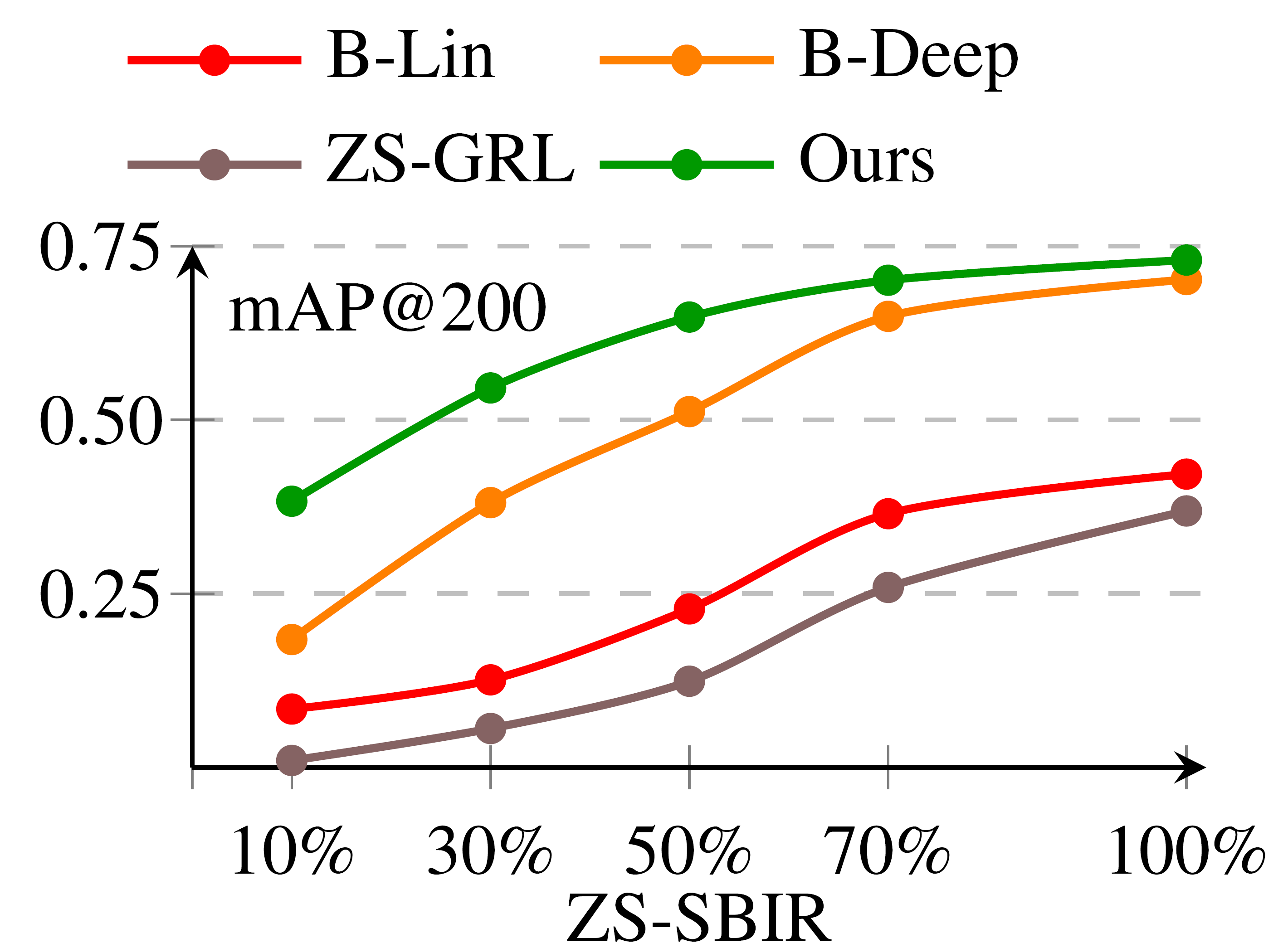
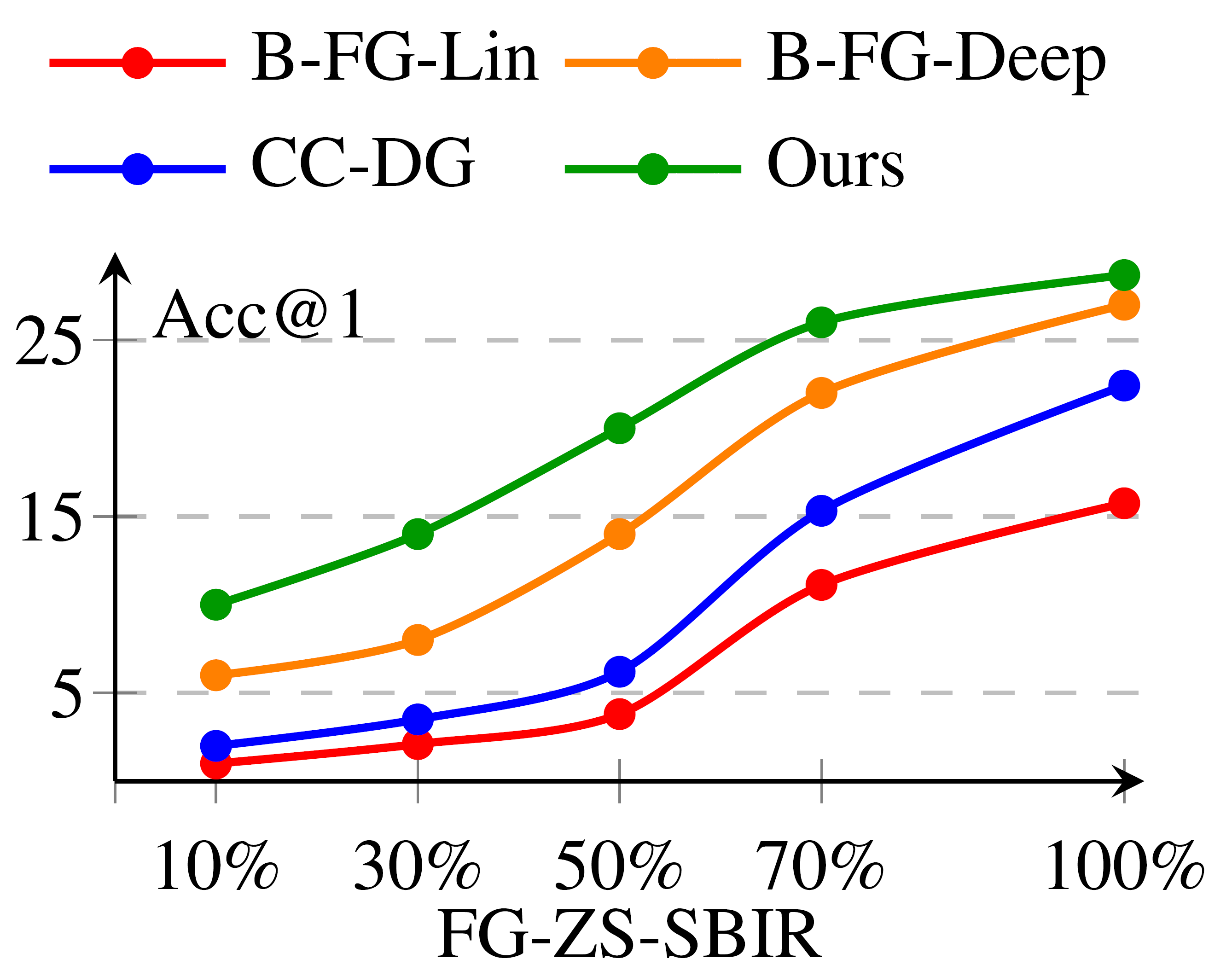
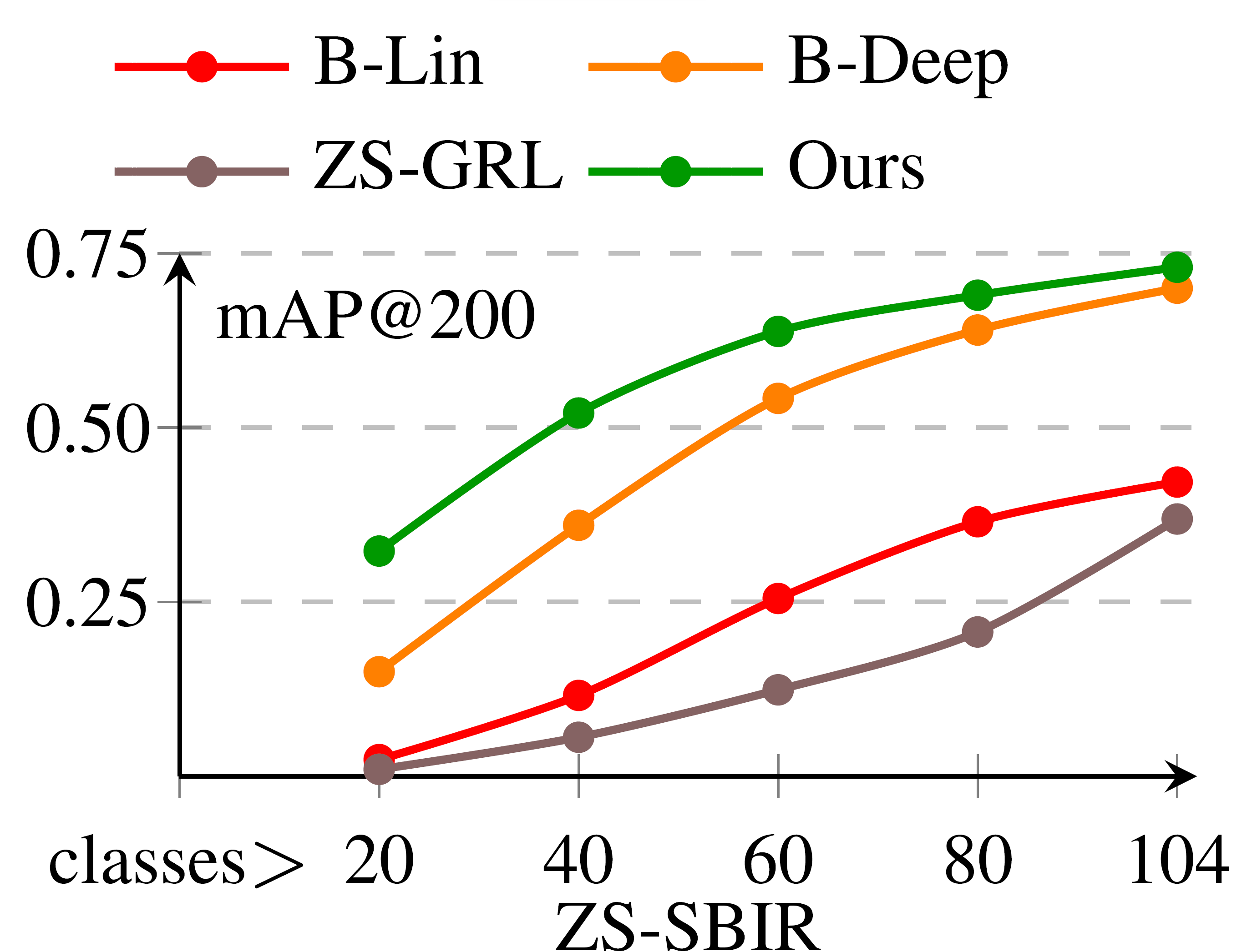
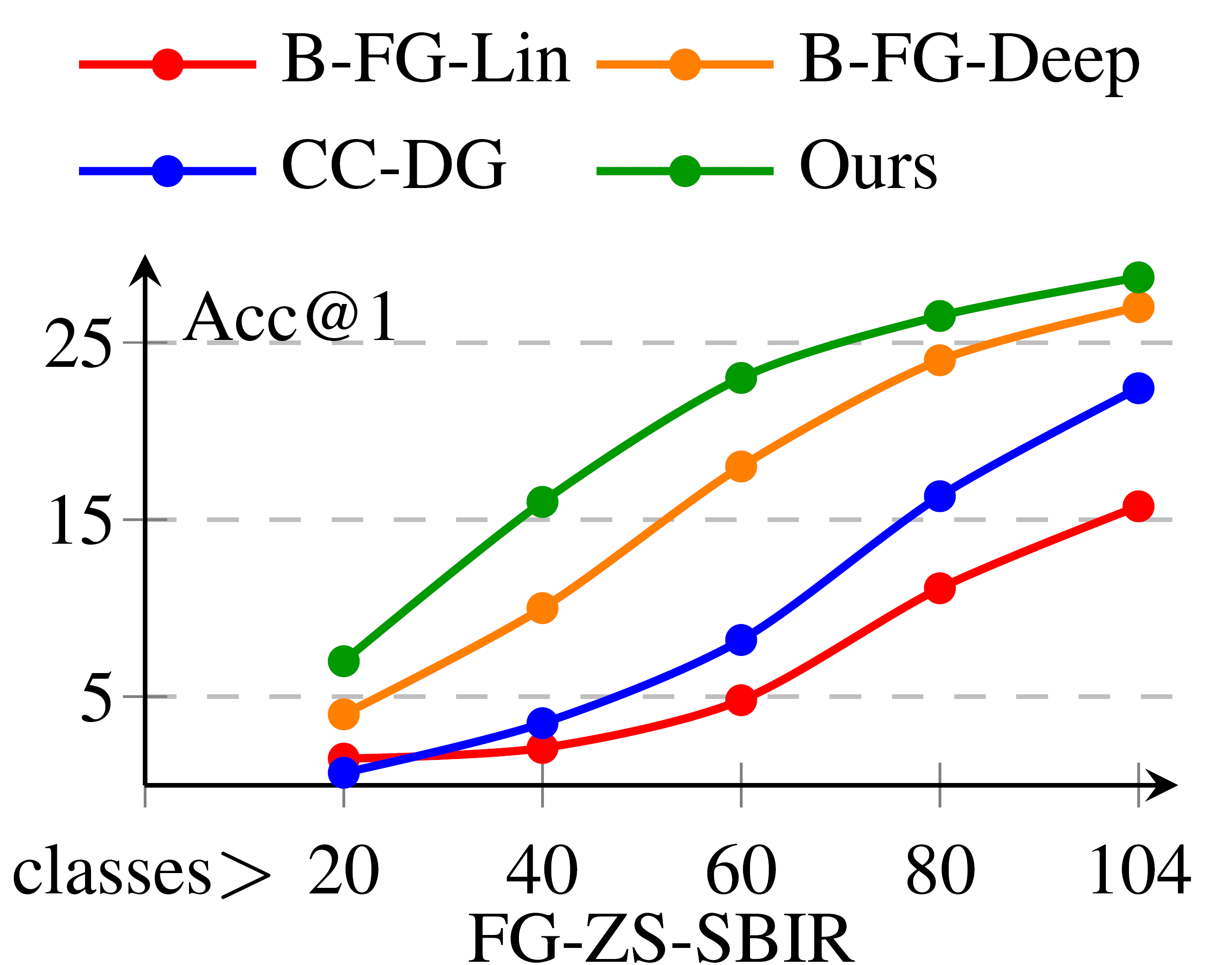
Figure 4: Plots showing extent of generalisation by varying training data-size (left two) and number of seen categories (right two).

Extent of Generalisation:  A strong motivation for using CLIP is its out-of-distribution performance [47] that promises to enable large-scale real-world deployment of sketch applications. Scrutinising this generalisation potential further, we experiment in two paradigms: (i) we vary training data per-class as 10%, 30%, 50%, 70% and 100%, and (ii) we vary number of seen classes as 20, 40, 60, 80 and 104 from Sketchy [53] respectively. Fig. 4 shows our ZS-SBIR and FG-ZS-SBIR performance to remain relatively stable at variable training-data-size (left) as well as across variable number of seen (training) categories (right), compared to prior arts and baselines, justifying the zero-shot potential of CLIP for both ZS-SBIR and FG-ZS-SBIR tasks.

6.3 Ablation Study

Justifying design components:  We evaluate our models, dropping one component at a time (Table 2) for both ZS-SBIR and FG-ZS-SBIR. While not fine-tuning LayerNorm (w/o LayerNorm) lowers performance on both paradigms slightly, removing $\mathcal{L}^{\mathcal{I}}_{\text{cls}}$ (w/o f-Divergene) severely affects FG-ZS-SBIR as it loses it class-discrimination ability. Removing $\mathcal{L}_{\text{PS}}$ (w/o Patch-Shuffling) and $\mathcal{L}_{\delta}$ (w/o f-Divergence) lowers FG-ZS-SBIR accuracy by 3.15% and 3.75%, owing to loss of sketch-photo structural correspondence and non-uniform relative sketch-photo distances across categories, thus verifying contribution of every design choice. Furthermore, using $2\times 2$ patches instead of $3\times 3$ for FG-ZS-SBIR provides a 1.2% gain in Acc.@1 (Sketchy), thus being optimal, as larger grid means more white patches for sketch, leading to confused embeddings.

Table 2: Ablation Study on Sketchy

Methods	ZS-SBIR		FG-ZS-SBIR
	mAP@all	P@200	Top-1	Top-5
w/o LayerNorm	0.698	0.701	27.18	59.55
w/o Classification ($\mathcal{L}^{\mathcal{I}}_{\text{cls}}$)	0.703	0.710	10.69	16.32
w/o Patch-Shuffling ($\mathcal{L}_{\text{PS}}$)	–	–	25.18	53.07
w/o f-Divergence ($\mathcal{L}_{\delta}$)	–	–	24.93	53.72
Ours	0.723	0.725	28.68	62.34

CLIP text encoder v/s Word2vec:  Unlike earlier works [16] that obtained semantics of a category via reconstruction from word2vec [41] embeddings for that category, our method replaces it with feature embedding from CLIP’s text encoder [46]. Word2vec [41] is trained using text-only data, whereas CLIP’s text encoder trains on large-scale ($400M$) image-text pairs. Using word2vec embeddings in our proposed method instead, drops performance by $4.57\%/0.172$ (Acc@1/mAP@200) for ZS-SBIR/FG-ZS-SBIR on Sketchy [53], justifying our choice of CLIP’s text encoder, capturing visual-semantic association (text-photo pairs) instead of text-only information (word2vec).

Should we learn text prompts?:  While handcrafted prompt templates like ‘a photo of a [category]’ works well for class-discrimination training (Eqn. 4), we wish to explore if there is any need to learn text prompts like our visual prompts. Consequently, following [75] we take $N$ learnable prompts, matching the word embeddings of handcrafted prompt dimensionally for the $i^{\text{th}}$ class as: $\eta^{t}=\{\eta_{1},\eta_{2},\cdots,\eta_{N},c_{i}\}$ with word embedding $c_{i}$ denoting the class name [75]. Training accordingly, drops performance by $2.36\%/0.078$ (Acc.@1/mAP@200) in Sketchy for ZS-SBIR/ZS-SBIR. This is probably because unlike learned prompts, handcrafted prompts being rooted in natural language vocabulary are inclined to have a higher generalisation ability in our case than learned text-prompts [41].

Varying number of Prompts:   To ensure that our visual prompt ($\mathbb{R}^{K\times d_{p}}$) has sufficient information capacity [64], we experiment with $K$ = $\{1,2,3,4\}$. Accuracy improves from $26.15\%/0.675$ at $K$ = 1 to $28.68\%/0.723$ at $K$ = 3, but saturates to $28.26\%/0.718$ (Acc@1/mAP@200) at $K$ = 4 on Sketchy, proving optimal $K$ as 3. We conjecture that a high capacity prompt might lead to over-fitting [76] of CLIP thus resulting in a lower zero-shot performance.

Comparing text-based image retrieval:  To explore how sketch fares against keywords as a query in a zero-shot retrieval paradigm, we compare keyword-based retrieval against ZS-SBIR on Sketchy(ext), and against FG-ZS-SBIR on Song et al.’s [59] dataset having fine-grained sketch-photo-text triplets for fine-grained retrieval. While keyword based retrieval employed via off-the-shelf CLIP, remains competitive ($0.523/0.612$ mAP/P@200) against our ZS-SBIR framework ($0.723/0.725$), it lags behind substantially ($4.6\%$ Acc@1) from our ZS-FG-SBIR method ($18.68\%$ Acc@1), proving the well-accepted superiority of sketch in modelling fine-grained details over text [70].

7 Conclusion

In this work we leverage CLIP’s open-vocab generalisation potential via an intuitive prompt-based design to enhance zero-shot performance of SBIR – both category-level and fine-grained, where our method surpasses all prior state-of-the-arts significantly. Towards improving fine-grained ZS-SBIR, we put forth two novel strategies of making relative sketch-photo feature distances across categories uniform and learning structural sketch-photo correspondences via a patch-shuffling technique. Last but not least, we hope to have informed the sketch community on the potential of synergizing foundation models like CLIP and sketch-related tasks going forward.

A Prompt Design for ZS-SBIR and ZS-FG-SBIR

Here we show in detail the way visual prompts are incorporated into the Image Encoder of CLIP [46].

For ZS-SBIR, we have two separate CLIP-image-encoders for photo and sketch branch with sketch and photo prompts incorporated into the respective encoders. During training the entire CLIP model is kept frozen except the LayerNorm of transformer layers and the prompts themselves, as shown in Fig. 5.

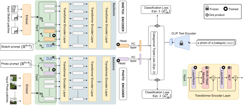
Figure 5: Prompt Design for ZS-SBIR along with training objectives.

For FG-ZS-SBIR, we use one CLIP-image-encoder with one common prompt shared for both photo and sketch branches incorporated into the CLIP-image encoder. Similar to ZS-SBIR design, during training the entire CLIP model is kept frozen except the LayerNorm of transformer layers and the prompt itself, as shown in Fig. 6. Apart from shared image-encoders the main difference from ZS-SBIR is in considering hard-triplets within each category instead of category-level triplets as in ZS-SBIR. Furthermore, we have two more additional losses apart from the ones used for ZS-SBIR, aimed at (i) making the relative sketch-photo distances across categories uniform via f-divergence, and (ii) learning the structural correspondences between a sketch-photo pair via Patch-shuffling loss.

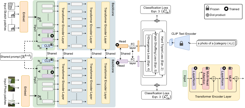
Figure 6: Prompt Design for FG-ZS-SBIR along with training objectives.

B Datasets

For evaluation on ZS-SBIR we have used three datasets:

(i) Sketchy (extended) [35] – Sketchy [53] contains 75,471 sketches over 125 categories having 100 images per category, with atleast 5 associated hand-drawn sketches per photo [69]. It was extended [35] further with extra 60,502 images from ImageNet [48] (Sketchy-ext), which we use here. Following [69] for zero-shot setup we split it as 104 classes for training and 21 for testing, ensuring that test-set images do not overlap with 1000 classes of ImageNet [48].

(ii) TUBerlin [20] – contains 250 categories, with 80 free-hand sketches in each, which was extended with a total of 204,489 images by [72]. We split it following [16] as 30 classes for testing and 220 for training.

(iii) QuickDraw Extended – The full-version contains over 50 million sketches across 345 categories, drawn by users across the internet under 20 seconds per sketch. Augmenting the sketches with images from Flickr, a subset of QuickDraw with 110 categories having 330,000 sketches and 204,000 photos was introduced for ZS-SBIR in [16]. We follow their split of 80 classes for training and 30 for testing to ensure no overlap of test-set photos from ImageNet [48].

For evaluation on FG-ZS-SBIR we require fine-grained (one-to-one matching) sketch-photo association [70] across categories for evaluation. Accordingly we resort to Sketchy [53] which has atleast atleast 5 associated hand-drawn sketches associated to every photo [69]. We use the same zero-shot categorical split of 104 training and 21 testing classes [69]. A few examples of sketch-photo association with multiple sketches per photo is illustrated in Fig. 7.

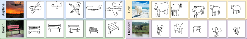
Figure 7: Some examples of Fine-grained associations across categories from Sketchy [53].

C More on f-Divergence

To use a single (global) margin parameter $\mu$ that works for all categories, we impose a regulariser that aims to make the sketch-photo relative distance, defined as $\delta(s,p^{+},p^{-})$, uniform across categories. We achieve this by computing the distribution of relative distances for all triplets $(s,p^{+},p^{-})$ in category $c$ as $\mathcal{D}_{c}=\{\delta(s_{i},p^{+}_{i},p^{-}_{i})\}_{i=1}^{N_{s}}$, where the $c^{th}$ category has $N_{s}$ sketch-photo pairs. Next, towards making the relative distance uniform across all categories, we minimise the KL-divergence [34] between a distribution of relative distances.

However, KL-divergence [34] only computes the information distance between two distributions – the length of the shortest program to describe a second distribution given the first. Comparing multiple $(\geq 2)$ distributions however is comparatively less studied. The multi-distribution generalisation of information distance, aka., the $f$-divergence is defined by a convex function $f:[0,\infty)\rightarrow\mathbb{R}$. Despite its generalisation capability, $f$-divergence for multiple distribution setup is under-explored in computer vision applications. In this paper, we thus adopt a rather simplistic definition of $f$-divergence by Sgarro [54] – the average divergence, which is defined as,

$$\frac{1}{N_{s}(N_{s}-1)}\sum_{i=1}^{N_{s}}\sum_{j=1}^{N_{s}}\texttt{KL}(\mathcal{D}_{i},\mathcal{D}_{j})$$ (6)

D Some Qualitative Results on Sketchy

Figures show qualitative results on Sketchy (ext) [35] for ZS-SBIR (Fig. 8) and on Sketchy [53] for FG-ZS-SBIR (Fig. 9), of baseline methods vs. ours. Baselines are constructed following [16] and [70] for ZS-SBIR and FG-ZS-SBIR respectively.

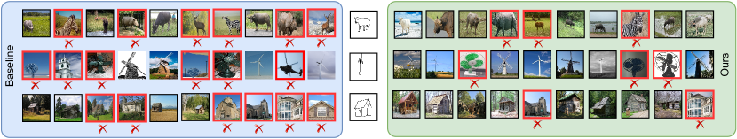
Figure 8: Qualitative results of ZS-SBIR on Sketchy [35] by a baseline (blue) method vs Ours (green).

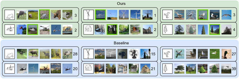
Figure 9: Qualitative results of FG-ZS-SBIR on Sketchy [53] by a baseline (blue) method vs Ours (green). The images are arranged in increasing order of the ranks beside their corresponding sketch-query, i.e the left-most image was retrieved at rank-1 for every category. The true-match for every query, if appearing in top-5 is marked in a green frame. Numbers denote the rank at which that true-match is retrieved for every corresponding sketch-query.

E Limitations

We observed two plausible limitations of our method which we keep for addressal in a future work. (i) The assumption that CLIP covers almost all classes during training, might fail in certain niche cases. (ii) Being trained on internet-scale data (400M image-text pairs), thorough zero-shot evaluation on an unseen class is challenging. However both limitations are universal to all CLIP-based applications.

References

- [1] Rameen Abdal, Peihao Zhu, John Femiani, Niloy Mitra, and Peter Wonka. Clip2stylegan: Unsupervised extraction of stylegan edit directions. In ACM TOG, 2022.
- [2] Ryan Prescott Adams and Richard S. Zemel. Ranking via sinkhorn propagation. arXiv preprint arXiv:1106.1925, 2011.
- [3] Hyojin Bahng, Ali Jahanian, Swami Sankaranarayanan, and Phillip Isola. Visual prompting: Modifying pixel space to adapt pre-trained models. arXiv preprint arXiv:2203.17274, 2022.
- [4] Alberto Baldrati, Marco Bertini, Tiberio Uricchio, and Alberto Del Bimbo. Effective conditioned and composed image retrieval combining clip-based features. In CVPR, 2022.
- [5] Ayan Kumar Bhunia, Pinaki Nath Chowdhury, Aneeshan Sain, Yongxin Yang, Tao Xiang, and Yi-Zhe Song. More photos are all you need: Semi-supervised learning for fine-grained sketch based image retrieval. In CVPR, 2021.
- [6] Ayan Kumar Bhunia, Subhadeep Koley, Abdullah Faiz Ur Rahman Khilji, Aneeshan Sain, Pinaki Nath Chowdhury, Tao Xiang, and Yi-Zhe Song. Sketching without worrying: Noise-tolerant sketch-based image retrieval. In CVPR, 2022.
- [7] Ayan Kumar Bhunia, Subhadeep Koley, Amandeep Kumar, Aneeshan Sain, Pinaki Nath Chowdhury, Tao Xiang, and Yi-Zhe Song. Sketch2Saliency: Learning to Detect Salient Objects from Human Drawings. In CVPR, 2023.
- [8] Ayan Kumar Bhunia, Aneeshan Sain, Parth Hiren Shah, Animesh Gupta, Pinaki Nath Chowdhury, Tao Xiang, and Yi-Zhe Song. Adaptive fine-grained sketch-based image retrieval. In ECCV, 2022.
- [9] Ayan Kumar Bhunia, Yongxin Yang, Timothy M Hospedales, Tao Xiang, and Yi-Zhe Song. Sketch less for more: On-the-fly fine-grained sketch based image retrieval. In CVPR, 2020.
- [10] Tom Brown, Benjamin Mann, Nick Ryder, Melanie Subbiah, Jared D Kaplan, Prafulla Dhariwal, Arvind Neelakantan, Pranav Shyam, Girish Sastry, Amanda Askell, et al. Language models are few-shot learners. NeurIPS, 2020.
- [11] Zhaoxi Chen, Guangcong Wang, and Ziwei Liu. Text2light: Zero-shot text-driven hdr panorama generation. ACM TOG, 2022.
- [12] Pinaki Nath Chowdhury, Ayan Kumar Bhunia, Aneeshan Sain, Subhadeep Koley, Tao Xiang, and Yi-Zhe Song. SceneTrilogy: On Human Scene-Sketch and its Complementarity with Photo and Text. In CVPR, 2023.
- [13] Pinaki Nath Chowdhury, Ayan Kumar Bhunia, Aneeshan Sain, Subhadeep Koley, Tao Xiang, and Yi-Zhe Song. What Can Human Sketches Do for Object Detection? In CVPR, 2023.
- [14] John Collomosse, Tu Bui, and Hailin Jin. Livesketch: Query perturbations for guided sketch-based visual search. In CVPR, 2019.
- [15] Jacob Devlin, Ming-Wei Chang, Kenton Lee, and Kristina Toutanova. Bert: Pre-training of deep bidirectional transformers for language understanding. In NAACL, 2019.
- [16] Sounak Dey, Pau Riba, Anjan Dutta, Josep Llados, and Yi-Zhe Song. Doodle to search: Practical zero-shot sketch-based image retrieval. In CVPR, 2019.
- [17] Alexey Dosovitskiy, Lucas Beyer, Alexander Kolesnikov, Dirk Weissenborn, Xiaohua Zhai, Thomas Unterthiner, Mostafa Dehghani, Matthias Minderer, Georg Heigold, Sylvain Gelly, Jakob Uszkoreit, and Neil Houlsby. An image is worth 16x16 words: Transformers for image recognition at scale. In ICLR, 2021.
- [18] Anjan Dutta and Zeynep Akata. Semantically tied paired cycle consistency for zero-shot sketch-based image retrieval. In CVPR, 2019.
- [19] Anjan Dutta and Zeynep Akata. Semantically tied paired cycle consistency for zero-shot sketch-based image retrieval. In CVPR, 2019.
- [20] Mathias Eitz, James Hays, and Marc Alexa. How do humans sketch objects? ACM TOG, 2012.
- [21] Jonathan Frankle, David J. Schwab, and Ari S. Morcos. Training batchnorm and only batchnorm: On the expressive power of random features. In ICLR, 2021.
- [22] Peng Gao, Shijie Geng, Renrui Zhang, Teli Ma, Rongyao Fang, Yongfeng Zhang, Hongsheng Li, and Yu Qiao. Clip-adapter: Better vision-language models with feature adapters. arXiv preprint arXiv:2110.04544, 2021.
- [23] Darío Garćia-Garćia and Robert C. Williamson. Divergences and risks for multiclass experiments. In CoLT, 2012.
- [24] Xiuye Gu, Tsung-Yi Lin, Weicheng Kuo, and Yin Cui. Open-vocabulary object detection via vision and language knowledge distilation. In ICLR, 2022.
- [25] David Ha and Douglas Eck. A neural representation of sketch drawings. In ICLR, 2018.
- [26] Kaiming He, Xiangyu Zhang, Shaoqing Ren, and Jian Sun. Deep residual learning for image recognition. In CVPR, 2016.
- [27] Timothy Hospedales, Antreas Antoniou, Paul Micaelli, and Amos Storkey. Meta-learning in neural networks: A survey. IEEE TPAMI, 2022.
- [28] HyeongJoo Hwang, Geon-Hyeong Kim, Seunghoon Hong, and Kee-Eung Kim. Variational interaction information maximization for cross-domain disentanglement. In NeurIPS, 2020.
- [29] Menglin Jia, Luming Tang, Bor-Chun Chen, Claire Cardie, Serge Belongie, Bharath Hariharan, and Ser-Nam Lim. Visual prompt tuning. In ECCV, 2022.
- [30] Muhammad Uzair Khattak, Hanoona Rasheed, Muhammad Maaz, Salman Khan, and Fahad Shahbaz Khan. Maple: Multi-modal prompt learning. arXiv preprint arXiv:2210.03117, 2022.
- [31] Konwoo Kim, Michael Laskin, Igor Mordatch, and Deepak Pathak. How to adapt your large-scale vision-and-language model. https://openreview.net/forum?id=EhwEUb2ynIa, 2022.
- [32] Subhadeep Koley, Ayan Kumar Bhunia, Aneeshan Sain, Pinaki Nath Chowdhury, Tao Xiang, and Yi-Zhe Song. Picture that Sketch: Photorealistic Image Generation from Abstract Sketches. In CVPR, 2023.
- [33] Alex Krizhevsky, Ilya Sutskever, and Geoffrey E Hinton. Imagenet classification with deep convolutional neural networks. In NeurIPS, 2012.
- [34] Solomon Kullback and Richard Leibler. On information and sufficiency. The Annals of Mathematical Statistics, 1951.
- [35] Li Liu, Fumin Shen, Yuming Shen, Xianglong Liu, and Ling Shao. Deep sketch hashing: Fast free-hand sketch-based image retrieval. In CVPR, 2017.
- [36] Pengfei Liu, Weizhe Yuan, Jinlan Fu, Zhengbao Jiang, Hiroaki Hayashi, and Graham Neubig. Pre-train, prompt, and predict: A systematic survey of prompting methods in natural language processing. ACM Computing Surveys, 2022.
- [37] Qing Liu, Lingxi Xie, Huiyu Wang, and Alan Yuille. Semantic-aware knowledge preservation for zero-shot sketch-based image retrieval. In ICCV, 2019.
- [38] Chong Long, Xiaoyan Zhu, Ming Li, and Bin Ma. Information shared by many objects. In CIKM, 2008.
- [39] Huaishao Luo, Lei Ji, Ming Zhong, Yang Chen, Wen Lei, Nan Duan, and Tianrui Li. Clip4clip: An empirical study of clip for end to end video clip retrieval. Neurocomputing, 2022.
- [40] Alexander G de G Matthews, James Hensman, Richard Turner, and Zoubin Ghahramani. On sparse variational methods and the kullback-leibler divergence between stochastic processes. In AISTATS, 2016.
- [41] Tomas Mikolov, Kai Chen, Greg Corrado, and Jeffrey Dean. Efficient estimation of word representations in vector space. In ICLR Workshop Poster, 2013.
- [42] Kaiyue Pang, Ke Li, Yongxin Yang, Honggang Zhang, Timothy M Hospedales, Tao Xiang, and Yi-Zhe Song. Generalising fine-grained sketch-based image retrieval. In CVPR, 2019.
- [43] Kaiyue Pang, Yi-Zhe Song, Tony Xiang, and Timothy M Hospedales. Cross-domain generative learning for fine-grained sketch-based image retrieval. In BMVC, 2017.
- [44] Kaiyue Pang, Yongxin Yang, Timothy M Hospedales, Tao Xiang, and Yi-Zhe Song. Solving mixed-modal jigsaw puzzle for fine-grained sketch-based image retrieval. In CVPR, 2020.
- [45] Or Patashnik, Zongze Wu, Eli Shechtman, Daniel Cohen-Or, and Dani Lischinski. Styleclip: Text-driven manipulation of stylegan imagery. In ICCV, 2021.
- [46] Alec Radford, Jong Wook Kim, Chris Hallacy, Aditya Ramesh, Gabriel Goh, Sandhini Agarwal, Girish Sastry, Amanda Askell, Pamela Mishkin, Jack Clark, et al. Learning transferable visual models from natural language supervision. In ICML, 2021.
- [47] Yongming Rao, Wenliang Zhao, Guangyi Chen, Yansong Tang, Zheng Zhu, Guan Huang, Jie Zhou, and Jiwen Lu. Denseclip: Language-guided dense prediction with context-aware prompting. In CVPR, 2022.
- [48] Olga Russakovsky, Jia Deng, Hao Su, Jonathan Krause, Sanjeev Satheesh, Sean Ma, Zhiheng Huang, Andrej Karpathy, Aditya Khosla, Michael Bernstein, et al. Imagenet large scale visual recognition challenge. IJCV, 2015.
- [49] Aneeshan Sain, Ayan Kumar Bhunia, Subhadeep Koley, Pinaki Nath Chowdhury, Soumitri Chattopadhyay, Tao Xiang, and Yi-Zhe Song. Exploiting Unlabelled Photos for Stronger Fine-Grained SBIR. In CVPR, 2023.
- [50] Aneeshan Sain, Ayan Kumar Bhunia, Vaishnav Potlapalli, Pinaki Nath Chowdhury, Tao Xiang, and Yi-Zhe Song. Sketch3t: Test-time training for zero-shot sbir. In CVPR, 2022.
- [51] Aneeshan Sain, Ayan Kumar Bhunia, Yongxin Yang, Tao Xiang, and Yi-Zhe Song. Cross-modal hierarchical modelling forfine-grained sketch based image retrieval. In BMVC, 2020.
- [52] Aneeshan Sain, Ayan Kumar Bhunia, Yongxin Yang, Tao Xiang, and Yi-Zhe Song. Stylemeup: Towards style-agnostic sketch-based image retrieval. In CVPR, 2021.
- [53] Patsorn Sangkloy, Nathan Burnell, Cusuh Ham, and James Hays. The sketchy database: learning to retrieve badly drawn bunnies. ACM TOG, 2016.
- [54] Andrea Sgarro. Information divergence and the dissimilarity of probability distributions. Calcodo, 1981.
- [55] Shiv Shankar, Vihari Piratla, Soumen Chakrabarti, Siddhartha Chaudhuri, Preethi Jyothi, and Sunita Sarawagi. Generalizing across domains via cross-gradient training. In ICLR, 2018.
- [56] Claude E. Shannon. A mathematical theory of communication. Bell System Technical Journal, 1948.
- [57] Robin Sibson. Information radius. Probability Theory and Related Fields, 1969.
- [58] K. Simonyan and A. Zisserman. Very deep convolutional networks for large-scale image recognition. In ICLR, 2015.
- [59] Jifei Song, Yi-Zhe Song, Tony Xiang, and Timothy M Hospedales. Fine-grained image retrieval: the text/sketch input dilemma. In BMVC, 2017.
- [60] Jifei Song, Qian Yu, Yi-Zhe Song, Tao Xiang, and Timothy M Hospedales. Deep spatial-semantic attention for fine-grained sketch-based image retrieval. In ICCV, 2017.
- [61] Vishal Thengane, Salman Khan, Munawar Hayat, and Fahad Khan. Clip model is an efficient continual learner. arXiv preprint arXiv:2210.03114, 2022.
- [62] Jialin Tian, Xing Xu, Fumin Shen, Yang Yang, and Heng Tao Shen. Tvt: Three-way vision transformer through multi-modal hypersphere learning for zero-shot sketch-based image retrieval. In AAAI, 2022.
- [63] Jialin Tian, Xing Xu, Zheng Wang, Fumin Shen, and Xin Liu. Relationship-preserving knowledge distillation for zero-shot sketch based image retrieval. In ACM MM, 2021.
- [64] Naftali Tishby, Fernando C. Pereira, and William Bialek. The information bottleneck method. In 37th annual Allerton Conf. on Communication, Control, and Computing, 1999.
- [65] Hao Wang, Cheng Deng, Tongliang Liu, and Dacheng Tao. Transferable coupled network for zero-shot sketch-based image retrieval. IEEE TPAMI, 2021.
- [66] Kai Wang, Yifan Wang, Xing Xu, Xin Liu, Weihua Ou, and Huimin Lu. Prototype-based selective knowledge distillation for zero-shot sketch based image retrieval. In ACM MM, 2022.
- [67] Mengmeng Wang, Jiazheng Xing, and Yong Liu. Actionclip: A new paradigm for video action recognition. arXiv preprint arXiv:2109.08472, 2021.
- [68] Peng Xu, Yongye Huang, Tongtong Yuan, Kaiyue Pang, Yi-Zhe Song, Tao Xiang, Timothy M Hospedales, Zhanyu Ma, and Jun Guo. Sketchmate: Deep hashing for million-scale human sketch retrieval. In CVPR, 2018.
- [69] Sasi Kiran Yelamarthi, Shiva Krishna Reddy, Ashish Mishra, and Anurag Mittal. A zero-shot framework for sketch based image retrieval. In ECCV, 2018.
- [70] Qian Yu, Feng Liu, Yi-Zhe Song, Tao Xiang, Timothy M Hospedales, and Chen-Change Loy. Sketch me that shoe. In CVPR, 2016.
- [71] Qian Yu, Yongxin Yang, Feng Liu, Yi-Zhe Song, Tao Xiang, and Timothy M Hospedales. Sketch-a-net: A deep neural network that beats humans. IJCV, 2017.
- [72] Hua Zhang, Si Liu, Changqing Zhang, Wenqi Ren, Rui Wang, and Xiaochun Cao. Sketchnet: Sketch classification with web images. In CVPR, 2016.
- [73] Jingyi Zhang, Fumin Shen, Li Liu, Fan Zhu, Mengyang Yu, Ling Shao, Heng Tao Shen, and Luc Van Gool. Generative domain-migration hashing for sketch-to-image retrieval. In ECCV, 2018.
- [74] Zhaolong Zhang, Yuejie Zhang, Rui Feng, Tao Zhang, and Weiguo Fan. Zero-shot sketch-based image retrieval via graph convolution network. In AAAI, 2020.
- [75] Kaiyang Zhou, Jingkang Yang, Chen Change Loy, and Ziwei Liu. Conditional prompt learning for vision-language models. In CVPR, 2022.
- [76] Kaiyang Zhou, Jingkang Yang, Chen Change Loy, and Ziwei Liu. Learning to prompt for vision-language models. IJCV, 2022.
Supplementary material for