Patch-Mix Transformer for Unsupervised Domain Adaptation: A Game Perspective –Appendix–

Abstract

In this supplementary material, we first prove theorem 1 in Section 1. Then, Section 2 introduces the details of the proposed method, and Section 3 shows the algorithm of the proposed PMTrans. Section 4 and Section 5 show the results, analyses, and ablation experiments to prove the effectiveness of the proposed PMTrans. Finally, Section 6 shows some discussions and details about our proposed work.

1 Proof

1.1 Domain Distribution Estimation with PatchMix

Let $\mathcal{H}$ denote the representation spaces with dimensionality $\operatorname{dim}(\mathcal{H})$, $\mathcal{F}$ denote the set of encoding functions i.e., the feature extractor and $\mathcal{C}$ be the set of decoding functions i.e. the classifier. Let $\mathcal{P}_{\lambda}$ be the set of functions to generate mixup ratio for building the intermediate domain. Furthermore, let $P_{S}$, $P_{T}$, and $P_{I}$ be the empirical distributions of data $\mathcal{D}_{s}$, $\mathcal{D}_{t}$, and $\mathcal{D}_{i}$. Define $f^{\star}\in\mathcal{F},c^{\star}\in\mathcal{C},$ and $\mathcal{P}_{\lambda}^{\star}\in\mathcal{P}_{\lambda}$ be the minimizers of Eq. 1 and $D(P_{S},P_{T})$ as the measure of the domain divergence between $P_{S}$ and $P_{T}$:

$$D(P_{S},P_{T})= \inf_{f\in\mathcal{F},c\in\mathcal{C},\mathcal{P}_{\lambda}\in\mathcal{P}}\underset{(\bm{x}^{s},\bm{y}^{s}),\left(\bm{x}^{t},\bm{y}^{t}\right)}{\mathbb{E}}$$ (1)

$$\ell\left(c\left(\mathcal{P}_{\lambda}\left(f(\bm{x}^{s}),f\left(\bm{x}^{t}\right)\right)\right),\mathcal{P}_{\lambda}\left(\bm{y}^{s},\bm{y}^{t}\right)\right),$$

where $\ell$ is the CE loss. Then, we can reformulate Eq.1 as:

$$D\left(P_{S},P_{T}\right)=\inf_{\bm{h}_{1}^{s},\ldots,\bm{h}_{n}^{s}\in\mathcal{H}^{s},\bm{h}_{1}^{t},\ldots,\bm{h}_{n}^{t}\in\mathcal{H}^{t}}\frac{1}{n_{s}\times n_{t}}\sum_{i}^{n_{s}}\sum_{j}^{n_{t}}$$ (2)

$$\left\{\inf_{c\in\mathcal{C}}\int_{0}^{1}\ell\left(f\left(\mathcal{P}_{\lambda}\left(\bm{h}_{i}^{s},\bm{h}_{j}^{t}\right)\right),\mathcal{P}_{\lambda}\left(\bm{y}_{i}^{s},\bm{y}_{j}^{t}\right)\right)p(\lambda)\mathrm{d}\lambda\right\},$$

where $\bm{h}_{i}^{s}=f(\bm{x}^{s}_{i})$ and $\bm{h}_{j}^{t}=f(\bm{x}^{t}_{j})$. Inspired and borrowed by this work[23], we give proof as follows.

Theorem 1

:Let $d\in\mathbb{N}$ to represent the number of classes contained in three sets $\mathcal{D}_{s}$, $\mathcal{D}_{t}$, and $\mathcal{D}_{i}$. If $\operatorname{dim}(\mathcal{H})\geq d-1$, ${\mathcal{P}_{\lambda}}’\ell(c^{\star}(f^{\star}(\bm{x}_{i})),\bm{y}^{s})+(1-{\mathcal{P}_{\lambda}}^{\prime})\ell(c^{\star}(f^{\star}(\bm{x}_{i})),\bm{y}^{t})=0$, then $D\left(P_{S},P_{T}\right)=0$ and the corresponding minimizer $c^{\star}$ is a linear function from $\mathcal{H}$ to $\mathbb{R}^{d}$. Denote the scaled mixup ratio sampled from a learnable Beta distribution as $\mathcal{P}_{\lambda}’$.

Proof: First, the following statement is $\operatorname{true}$ if $\operatorname{dim}(\mathcal{H})\geq d-1$ :

$$\exists A,H\in\mathbb{R}^{\operatorname{dim}(\mathcal{H})\times d},b\in\mathbb{R}^{d}:A^{\top}H+b_{d}^{\top}=I_{d\times d},$$

where $I_{d\times d}$ and $1_{d}$ denote the $d$-dimensional identity matrix and all-one vector, respectively. In fact, $b_{d}^{\top}$ is a rank-one matrix, and the rank of the identity matrix is $d$. Since the column set span of $I_{d\times d}$ needs to be contained in the span of $A^{\top}H+b_{d}^{\top}$, $A^{\top}H$ only needs to be a matrix with the rank $d-1$ to meet this requirement.

Let $c^{\star}(h)=A^{\top}h+b$, for all $h\in\mathcal{H}$. Let $f^{\star}\left(\bm{x}_{i}^{s}\right)=H_{\zeta_{i}^{s},:}$ and $f^{\star}\left(\bm{x}_{j}^{t}\right)=H_{\zeta_{j}^{t},:}$ be the $\zeta_{i}$-th and $\zeta_{j}$-th slice of $H$, respectively. Specifically, $\zeta_{i}^{s},\zeta_{i}^{t}\in\{1,\ldots,d\}$ stand for the class-index of the examples $\bm{x}_{i}^{s}$ and $\bm{x}_{j}^{t}$. Given Eq.1, the intermediate domain sample $\bm{x}^{i}_{ij}=\mathcal{P}_{{\lambda}}^{\star}(\bm{a}_{i},\bm{b}_{j})=\mathcal{P}_{{\lambda}}^{\prime}\cdot\bm{a}_{i}+\left(1-{P}_{{\lambda}}^{\prime}\right)\cdot\bm{b}_{j}$, and the definition of cross-entropy loss $\ell$, we get:

$${{\mathcal{P}_{{\lambda}}}^{\prime}}\ell\left(c^{\star}\left(f^{\star}\left(\bm{x}^{i}_{ij}\right)\right),\bm{y}^{s}_{i}\right)+(1-{\mathcal{P}_{\lambda}}^{\prime})\ell\left(c^{\star}\left(f^{\star}\left(\bm{x}^{i}_{ij}\right)\right),\bm{y}^{t}_{j}\right)$$ (3)

$$=\ell\left(c^{\star}\left({\mathcal{P}_{{\lambda}}}^{\star}\left(f^{\star}\left(\bm{x}_{i}^{s}\right),f^{\star}\left(\bm{x}_{j}^{t}\right)\right)\right),{\mathcal{P}_{{\lambda}}}^{\star}\left(\bm{y}_{i}^{s},\bm{y}_{j}^{t}\right)\right)$$

$$=D\left(P_{S},P_{T}\right)=0.$$

Eq. 3 reveals that the source and target domains are aligned if mixing the patches from two domains is equivalent to mixing the corresponding labels.

Furthermore, we see the following:

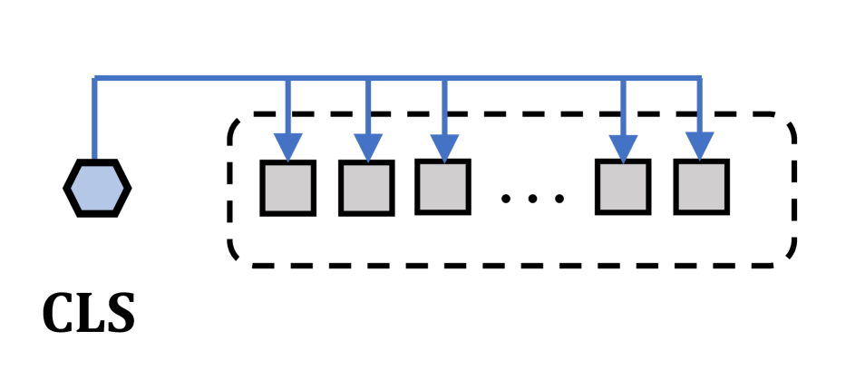
(a)

(b)

Figure 1: (a) Deit/ViT attention scores with the CLS token. (b) Swin attention scores with an output unit of Classifier that refers to $C_{i}$ . The dashed line denotes the sequence with each square representing a patch.

$$\ell\left(c^{\star}\left({\mathcal{P}_{\lambda}}^{\star}\left(f^{\star}\left(\bm{x}_{i}^{s}\right),f^{\star}\left(\bm{x}_{j}^{t}\right)\right)\right),{\mathcal{P}_{\lambda}}^{\star}\left(\bm{y}_{i}^{s},\bm{y}_{j}^{t}\right)\right)$$ (4)

$$=\ell\left(A^{\top}{\mathcal{P}_{\lambda}}^{\star}\left(H^{s}_{\zeta_{i},:},H^{t}_{\zeta_{j},:}\right)+b,{\mathcal{P}_{\lambda}}^{\star}\left(\bm{y}^{s}_{i,\zeta_{i}},\bm{y}^{t}_{j,\zeta_{j}}\right)\right)$$

$$=0.$$

The result follows from $A^{\top}H_{\zeta_{i}^{s},:}+b=y_{i,\zeta_{i}^{s}}\text{ for all }i\text{, }$ and $A^{\top}H_{\zeta_{j}^{t},:}+b=y_{i,\zeta_{j}^{t}}\text{ for all }j\text{. }$ If $\operatorname{dim}(\mathcal{H})\geq d-1$, $f^{\star}\left(\bm{x}_{i}^{t}\right)$ and $f^{\star}\left(\bm{x}_{j}^{t}\right)$ in the representation space $\mathcal{H}$ have some degrees of freedom to move independently. It also implies that when Eq. 3 is minimized, the representation of each class lies on a subspace of dimension $\operatorname{dim}(\mathcal{H})-d+1$, and with larger $dim(\mathcal{H})$, the majority of directions in $\mathcal{H}$-space will contain zero variance in the class-conditional manifold.

In practice, we utilize Eq. 3 to measure the domain gaps between the intermediate domain, and other domains and decrease them in the label and feature space, as illustrated in the main paper.

2 Details

2.1 Datasets

To evaluate the proposed method, we conduct extensive experiments on four popular UDA benchmarks, including Office-31 [17], Office-Home [22], VisDA-2017 [16], and DomainNet [15].

Office-31 consists of 4110 images of 31 categories, with three domains: Amazon (A), Webcam (W), and DSLR (D).

Office-Home is collected from four domains: Artistic images (A), Clip Art (C), Product images (P), and Real-World images (R) and consists of 15500 images from 65 classes.

VisDA-2017 is a more challenging dataset for synthetic-to-real domain adaptation. We set 152397 synthetic images as the source domain data and 55388 real-world images as the target domain data.

DomainNet is a large-scale benchmark dataset, which has 345 classes from six domains (Clipart (clp), Infograph (inf), Painting (pnt), Quickdraw (qdr), Real (rel), and Sketch (skt)).

2.2 Attention Map

We calculate the attention score in two ways based on whether the CLS token is present in the sequence. For Swin Transformer, we adopt a method similar to CAM [31] instead of changing the backbone from CNN to Transformer. Specifically, for a given image, let $f_{k}(x,y)$ represent the encoded patch $k$ in the last layer at spatial location $(x,y)$. The output of Transformer is followed by a global average pooling (GAP) layer$\sum(x,y)$ and a linear classification head. For the specific class $C_{i}$, the classification score $S_{C_{i}}$ is:

$$S_{C_{i}}=\sum_{j}w_{j}^{C_{i}}\sum_{x,y}f_{k}(x,y),$$ (5)

where $w_{j}^{C_{i}}$ represents the weight corresponding to class $C_{i}$ for unit $j$ in the hidden dimension. Eq.5 ensembles the semantics over both spatial contexts $\sum(x,y)$ and the linear head units $\sum(j)$. Then given Eq.5, as shown in Fig.1 (b), for a given $C_{i}$, we reallocate the semantic information from the output of linear head unit of $C_{i}$. In detail, we define the semantic activation map at location $(x,y)$ for a specific class $C_{i}$ as:

$$M_{C_{i}}(x,y)=\sum_{j}w_{j}^{C_{i}}f_{k}(x,y),$$

where $M_{C_{i}}\in\mathbb{R}^{2}$ is the activation for class $C_{i}$, and we infer $C_{i}$ by the ground-truth label in the source domain and the pseudo-label in the target domain to obtain the corresponding class activation map to build the intermediate domain. Then, we use $M_{C_{i}}$ as the attention map after the softmax operation.

On the other hand, when the CLS token is present in the output sequence of Transformer like Deit/ViT, we simply take the attention scores from the self-attention, i.e. the similarity matrix of each layer $i$ in Transformer $Attn_{i}\in\mathcal{R}^{H\times N\times N}$, and take the average in the head dimension $H$:

$$Attn_{i}=\frac{1}{H}\sum_{h}Attn_{h},$$

where $N$ is the sequence length. Next, we only take the CLS token’s attention after the softmax operation, as shown in Fig.1 (a), and then summarize each layer’s scores to obtain the final attention scores $Attn$.

$$Attn=\frac{1}{I}\sum_{i}Attn_{i}.$$

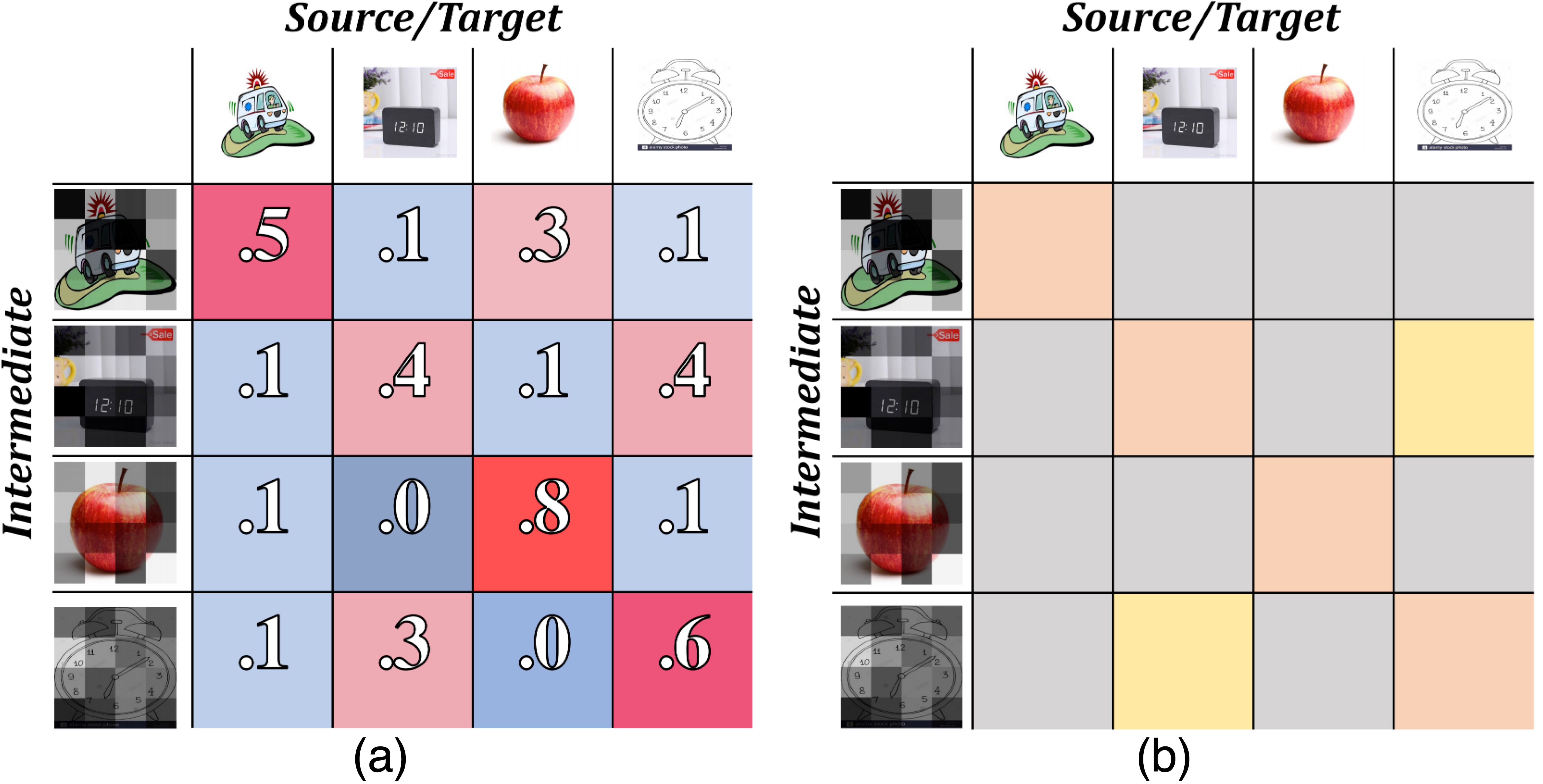
Figure 2: Illustration of the semi-supervised loss in feature space.

2.3 Semi-supervised mixup loss in the feature space

In Fig.2, we illustrate the semi-supervised loss in the feature space by similarity between features (in Fig. 2 (a)) and label spaces(in Fig.2 (b)). To compute the similarity of features, we use the normalized cosine similarity loss between the intermediate domain (column) and source/target domain(row) in the feature space, as shown in Fig.2(a). Each row denotes the normalized similarity between a sample of the intermediate domain and counterparts from the source domains. For example, we first use the cosine similarity to calculate the similarities between one intermediate sample ”car” and four sources (or target) samples (car, clock, apple, sketch clock). Then we normalize these similarities. As for the similarity of outputs (or) labels, since the source samples are labeled, and the target samples are unlabeled, we design two different methods to calculate the supervised and unsupervised label similarities. As for the label similarity between the intermediate and source domains, the intermediate and source samples both share the same labels. Therefore, we define the label similarity $\bm{y}^{is}=\bm{y}^{s}({\bm{y}^{s}})^{\intercal}$, as shown in Fig.2 (b). Specifically, $\bm{y}^{is}$, denoted by the yellow and pink colors, indicates that the label similarity between samples is one for these samples with the same labels (zero for different labels). For example, the label similarities between one intermediate sample ”sketch clock” and four sources (or target) samples car, clock, apple, and sketch clock are zero, one, zero, and one. As for the label similarity between the intermediate and target samples, we only know that the intermediate and source samples both share overlapped patches due to lack of supervision. Therefore, the label similarity $\bm{y}^{it}$ between samples with overlapped patches should be one (pink color), and others should be zero. And we define the label similarity $\bm{y}^{it}$ as identity matrix. For example, the label similarities between one unlabeled intermediate sample ”sketch clock” and four unlabeled target samples car, real clock, apple, and sketch clock are zero, zero, zero, and one. After obtaining the feature and label similarities, we utilize the CE loss $\ell$ to measure the discrepancy between these similarities as the domain gap between the intermediate and other domains.

2.4 Optimization

In our game, $m$-th player is endowed with a cost function $J_{m}$ and strives to reduce its cost, which contributes to the change of CE. We now define each player’s cost function $J_{m}$ as

$$\small\begin{split}J_{{\mathcal{F}}}\left(\bm{\omega}_{\mathcal{F}},\bm{\omega}_{-{\mathcal{F}}}\right)&:=\mathcal{L}_{cls}^{S}(\bm{\omega}_{\mathcal{F}},\bm{\omega}_{\mathcal{C}})+\alpha{CE}_{s,i,t}(\bm{\omega}),\\ J_{{\mathcal{C}}}\left(\bm{\omega}_{\mathcal{C}},\bm{\omega}_{-{\mathcal{C}}}\right)&:=\mathcal{L}_{cls}^{S}(\bm{\omega}_{\mathcal{F}},\bm{\omega}_{\mathcal{C}})+\alpha{CE}_{s,i,t}(\bm{\omega}),\\ J_{{\mathcal{P}}}\left(\bm{\omega}_{{\mathcal{P}}},\bm{\omega}_{-{\mathcal{P}}}\right)&:=-\alpha{CE}_{s,i,t}(\bm{\omega}),\end{split}$$ (6)

where $\alpha$ is the trade-off parameter, $\ell$ is the supervised classification loss for the source domain, and $\text{CE}_{s,i,t}(\bm{\omega})$ is the discrepancy between the intermediate domain and the source/target domain. To clarify the min-max process, we introduce the game’s vector field $v(w)$, which is identical to the gradient for every player.

Definition 1

(Vector field): .

$$v(\bm{\omega}):=(\bigtriangledown_{{\bm{\omega}}_{\mathcal{F}}}J_{\mathcal{F}},\bigtriangledown_{{\bm{\omega}}_{\mathcal{C}}}J_{\mathcal{C}},\bigtriangledown_{{\bm{\omega}}_{\mathcal{P}}}J_{\mathcal{P}})$$

By examining Definition.1 with respect to Eq.(6), the process can be categorized into both cooperation and competition [1].

$$v(w)=\begin{pmatrix}\bigtriangledown_{{\bm{\omega}}_{\mathcal{F}}}\mathcal{L}_{cls}^{S}(\bm{\omega}_{\mathcal{F}},\bm{\omega}_{\mathcal{C}})\\ \bigtriangledown_{{\bm{\omega}}_{\mathcal{C}}}\mathcal{L}_{cls}^{S}(\bm{\omega}_{\mathcal{F}},\bm{\omega}_{\mathcal{C}})\\ 0\end{pmatrix}+\begin{pmatrix}\alpha\bigtriangledown_{{\bm{\omega}}_{\mathcal{F}}}\text{CE}_{s,i,t}(\bm{\omega})\\ \alpha\bigtriangledown_{{\bm{\omega}}_{\mathcal{C}}}\text{CE}_{s,i,t}(\bm{\omega})\\ -\alpha\bigtriangledown_{{\bm{\omega}}_{\mathcal{P}}}\text{CE}_{s,i,t}(\bm{\omega})\end{pmatrix},$$ (7)

where the left part is related to the gradient of $\mathcal{L}_{cls}^{S}(\bm{\omega}_{\mathcal{F}},\bm{\omega}_{\mathcal{C}})$, and the right part denotes the adversarial behavior on producing or consuming CE in the network. In this Min-max CE Game, each player behaves selfishly to reduce their cost function. This competition on the network’s CE will possibly end with a situation where no one has anything to gain by changing only one’s strategy, called NE. Note that our method does not require explicit usage of gradient reverse layers as the prior GAN-based game design [6]. Our training is optimized as

$$v(\bm{\omega})=\bigtriangledown_{(\bm{\omega}_{\mathcal{F}},\bm{\omega}_{\mathcal{C}})}\mathcal{L}_{cls}^{S}(\bm{\omega}_{\mathcal{F}},\bm{\omega}_{\mathcal{C}})+\alpha\bigtriangledown_{{\bm{\omega}}}{CE}_{s,i,t}(\bm{\omega}).$$ (8)

2.5 Comparisons with Mixup variants

In Fig. 3, we show the visual comparisons between the PatchMix and mainstream Mixup variants. Mixup [28] mixes two samples by interpolating both the images and labels, which suffers from the local ambiguity. CutOut [4] proposes to randomly mask out square regions of input during training to improve the robustness of the CNNs. Since CutOut decreases the ImageNet localization or object detection performances, CutMix [27] is further introduced to randomly cut and paste the regions in an image, where the ground truth labels are also mixed proportionally to the area of the regions. However, sometimes there is no valid object in the mixed image due to the random process in augmentation, but there is still a response in the label space. Therefore, not all pixels are created equal, and the labels of pixels should be re-weighted. TransMix [2] is proposed to utilize the attention map to assign the confidence for the mixed samples and re-weighted the labels of pixels. In comparison, we unify these global and local mixup techniques in our PatchMix by learning to combine two patches to form a mixed patch and obtain mixed samples. Furthermore, we also learn the hyperparameters of the mixup ratio for each patch and effectively build up the intermediate domain samples.

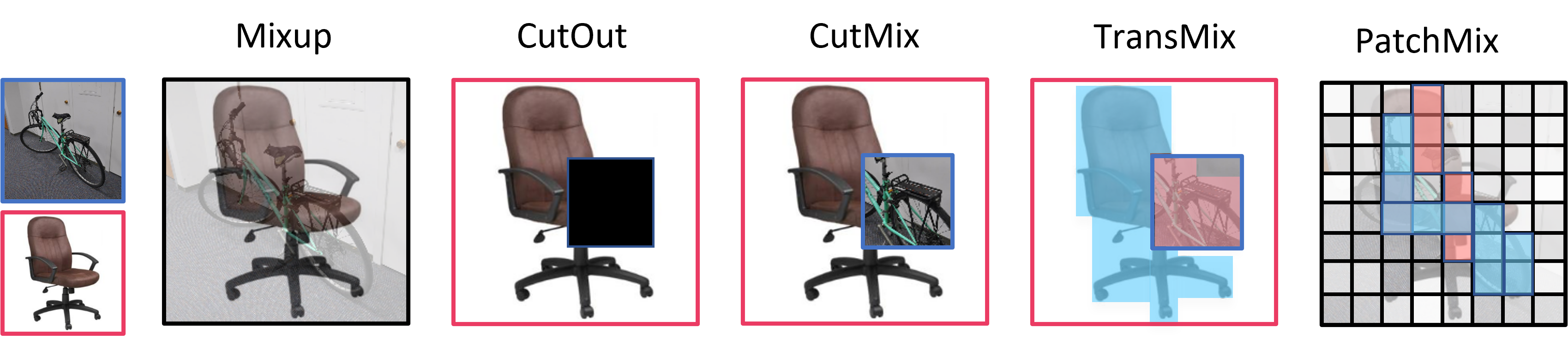
Figure 3: PMTrans and Mixup variants

3 Algorithm

In summary, the whole algorithm to train the proposed PMTrans is shown in Algorithm 1.

Algorithm 1 Patch-Mix Transformer for Unsupervised Domain Adaptation

0:  source domain data $\mathcal{D}_{s}$ and target domain data $\mathcal{D}_{t}$.

0:  learned parameters of feature extractor $\mathcal{\bm{\omega}}_{\mathcal{F}}$, classifier $\mathcal{\bm{\omega}}_{\mathcal{C}}$, and PatchMix $\mathcal{\bm{\omega}}_{\mathcal{P}}$.

1:  for $k=0$ to $\mathrm{MaxIter}$ do

2:     Sample a batch of input from source data and target data.

3:     Encode the patches of source and target inputs by the patch embedding (Emb) layer.

4:     Calculate the normalized attention score for each patch as Section 2.2.

5:     Sample the mixup ratio from Beta($\mathcal{\bm{\omega}}_{\mathcal{P}}$)

6:     Construct the intermediate domain input as shown in Eq. 9.

7:     Calculate the semi-supervised mixup loss in the feature space via Eq. 11.

8:     Calculate the semi-supervised mixup loss in the label space via Eq. 12.

9:     Measure the domain divergence between intermediate domain and other two domains via Eq. 14.

10:     Update network parameters $\bm{\omega}$ by optimization (8) via a AdamW [12] optimizer.

11:  end for

12:  return  $\mathcal{\bm{\omega}}_{\mathcal{F}}$, $\mathcal{\bm{\omega}}_{\mathcal{C}}$, and $\mathcal{\bm{\omega}}_{\mathcal{P}}$

where the related loss functions are shown as follows.

$$\small\begin{split}\bm{x}^{i}=\mathcal{P}_{\lambda}(\bm{x}^{s},\bm{x}^{t}),&~{}\bm{x}^{i}_{k}=\lambda_{k}\odot\bm{x}_{k}^{s}+(1-\lambda_{k})\odot\bm{x}_{k}^{t},\\ \bm{y}^{i}=\mathcal{P}_{\lambda}(\bm{y}^{s},\bm{y}^{t})&=\lambda^{s}\bm{y}^{s}+\lambda^{t}\bm{y}^{t}.\end{split}$$ (9)

$$\small\begin{split}\lambda^{s}&=\frac{\sum_{k=1}^{n}\lambda_{k}{a}_{k}^{s}}{\sum_{k=1}^{n}\lambda_{k}{a}_{k}^{s}+\sum_{k=1}^{n}(1-\lambda_{k}){a}_{k}^{t}},\\ \lambda^{t}&=\frac{\sum_{k=1}^{n}(1-\lambda_{k}){a}_{k}^{t}}{\sum_{k=1}^{n}\lambda_{k}{a}_{k}^{s}+\sum_{k=1}^{n}(1-\lambda_{k}){a}_{k}^{t}}.\end{split}$$ (10)

$$\small\begin{split}\mathcal{L}_{f}^{I,S}(\bm{\omega}_{\mathcal{F}},\bm{\omega}_{\mathcal{P}})=\mathbb{E}_{\left(\bm{x}^{i},\bm{y}^{i}\right)\sim D^{i}}\lambda^{s}\ell\left(d(\bm{x}^{i},\bm{x}^{s}),\bm{y}^{is}\right),\\ \mathcal{L}_{f}^{I,T}(\bm{\omega}_{\mathcal{F}},\bm{\omega}_{\mathcal{P}})=\mathbb{E}_{\left(\bm{x}^{i},\bm{y}^{i}\right)\sim D^{i}}\lambda^{t}\ell\left(d(\bm{x}^{i},\bm{x}^{t}),\bm{y}^{it}\right).\end{split}$$ (11)

$$\small\begin{split}\mathcal{L}_{l}^{I,S}(\bm{\omega})&=\mathbb{E}_{\left(\bm{x}^{i},\bm{y}^{i}\right)\sim D^{i}}\lambda^{s}\ell\left(\mathcal{C}\left(\mathcal{F}\left(\bm{x}^{i}\right)\right),\bm{y}^{s}\right),\\ \mathcal{L}_{l}^{I,T}(\bm{\omega})&=\mathbb{E}_{\left(\bm{x}^{i},\bm{y}^{i}\right)\sim D^{i}}\lambda^{t}\ell\left(\mathcal{C}\left(\mathcal{F}\left(\bm{x}^{i}\right)\right),\hat{\bm{y}^{t}}\right).\end{split}$$ (12)

$${\text{CE}}_{s,i,t}(\bm{\omega})=\mathcal{L}_{f}(\bm{\omega}_{\mathcal{F}},\bm{\omega}_{\mathcal{P}})+\mathcal{L}_{l}(\bm{\omega}).$$ (13)

$$J\left(\bm{\omega}\right):=\mathcal{L}_{cls}^{S}(\bm{\omega}_{\mathcal{F}},\bm{\omega}_{\mathcal{C}})+\alpha{\text{CE}}_{s,i,t}(\bm{\omega}).$$ (14)

Note that these above equations are introduced in detail in the main paper.

4 Results and Analyses

4.1 The comparisons on the Office-31, Office-Home, and VisDA-2017

We compare PMTrans with the SoTA methods, including ResNet- and ViT-based methods. The ResNet-based methods are FixBi [14], CGDM [5], MCD [18], SWD [9], SCDA [11], BNM [3], MDD [29], CKB [13], TSA [10], DWL [24], ILA [19], Symnets [30], CAN [8], and PCT [21]. The ViT-based methods are SSRT [20], CDTrans [25], and TVT [26], and we directly quote the results in their original papers for fair comparison. And the more detailed comparisons on three datasets are shown as Tab. 1, Tab. 2 , and Tab. 3.

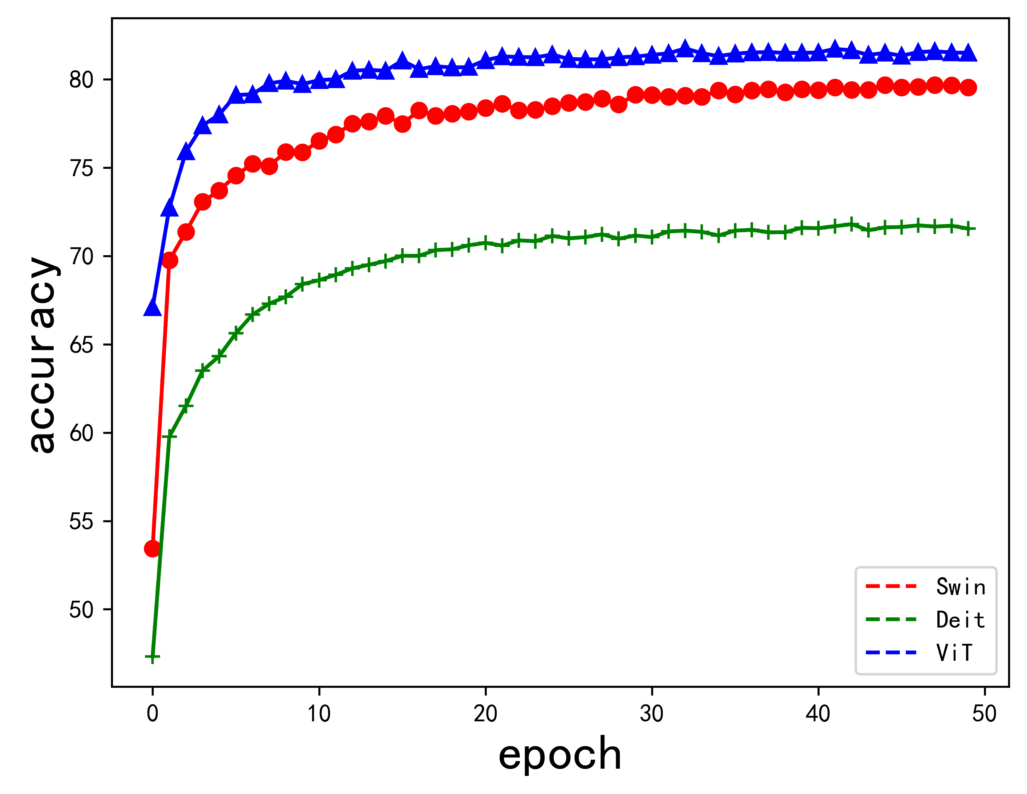
Figure 4: Accuracy on the task A $\to$ C (Office-Home)

Method		A $\to$ W	D$\to$ W	W$\to$ D	A$\to$ D	D$\to$ A	W$\to$ A	Avg
ResNet-50	ResNet	68.9	68.4	62.5	96.7	60.7	99.3	76.1
BNM		91.5	98.5	100.0	90.3	70.9	71.6	87.1
DWL		89.2	99.2	100.0	91.2	73.1	69.8	87.1
MDD		94.5	98.4	100.0	93.5	74.6	72.2	88.9
TSA		94.8	99.1	100.0	92.6	74.9	74.4	89.3
ILA+CDAN		95.7	99.2	100.0	93.4	72.1	75.4	89.3
PCT		94.6	98.7	99.9	93.8	77.2	76.0	90.0
SCDA		94.2	98.7	99.8	95.2	75.7	76.2	90.0
FixBi		96.1	99.3	100.0	95.0	78.7	79.4	91.4
TVT	ViT	96.4	99.4	100.0	96.4	84.9	86.0	93.9
Deit-Base		89.2	98.9	100.0	88.7	80.1	79.8	89.5
CDTrans-Deit		96.7	99.0	100.0	97.0	81.1	81.9	92.6
PMTrans-Deit		99.0	99.4	100.0	96.5	81.4	82.1	93.1
ViT-Base		91.2	99.2	100.0	90.4	81.1	80.6	91.1
SSRT-ViT		97.7	99.2	100.0	98.6	83.5	82.2	93.5
PMTrans-ViT		99.1	99.6	100.0	99.4	85.7	86.3	95.0
Swin-Base	Swin	97.0	99.2	100.0	95.8	82.4	81.8	92.7
PMTrans-Swin		99.5	99.4	100.0	99.8	86.7	86.5	95.3

Table 1: Comparison with SoTA methods on Office-31. The best performance is marked as bold.

Method		A$\to$ C	A$\to$ P	A $\to$ R	C $\to$ A	C $\to$ P	C $\to$ R	P$\to$ A	P$\to$ C	P$\to$ R	R$\to$ A	R$\to$ C	R$\to$ P	Avg
ResNet-50	ResNet	44.9	66.3	74.3	51.8	61.9	63.6	52.4	39.1	71.2	63.8	45.9	77.2	59.4
MCD		48.9	68.3	74.6	61.3	67.6	68.8	57.0	47.1	75.1	69.1	52.2	79.6	64.1
Symnets		47.7	72.9	78.5	64.2	71.3	74.2	64.2	48.8	79.5	74.5	52.6	82.7	67.6
MDD		54.9	73.7	77.8	60.0	71.4	71.8	61.2	53.6	78.1	72.5	60.2	82.3	68.1
TSA		53.6	75.1	78.3	64.4	73.7	72.5	62.3	49.4	77.5	72.2	58.8	82.1	68.3
CKB		54.7	74.4	77.1	63.7	72.2	71.8	64.1	51.7	78.4	73.1	58.0	82.4	68.5
BNM		56.7	77.5	81.0	67.3	76.3	77.1	65.3	55.1	82.0	73.6	57.0	84.3	71.1
PCT		57.1	78.3	81.4	67.6	77.0	76.5	68.0	55.0	81.3	74.7	60.0	85.3	71.8
FixBi		58.1	77.3	80.4	67.7	79.5	78.1	65.8	57.9	81.7	76.4	62.9	86.7	72.7
TVT	ViT	74.9	86.8	89.5	82.8	88.0	88.3	79.8	71.9	90.1	85.5	74.6	90.6	83.6
Deit-Base		61.8	79.5	84.3	75.4	78.8	81.2	72.8	55.7	84.4	78.3	59.3	86.0	74.8
CDTrans-Deit		68.8	85.0	86.9	81.5	87.1	87.3	79.6	63.3	88.2	82.0	66.0	90.6	80.5
PMTrans-Deit		71.8	87.3	88.3	83.0	87.7	87.8	78.5	67.4	89.3	81.7	70.7	92.0	82.1
ViT-Base		67.0	85.7	88.1	80.1	84.1	86.7	79.5	67.0	89.4	83.6	70.2	91.2	81.1
SSRT-ViT		75.2	89.0	91.1	85.1	88.3	89.9	85.0	74.2	91.2	85.7	78.6	91.8	85.4
PMTrans-ViT		81.2	91.6	92.4	88.9	91.6	93.0	88.5	80.0	93.4	89.5	82.4	94.5	88.9
Swin-Base	Swin	72.7	87.1	90.6	84.3	87.3	89.3	80.6	68.6	90.3	84.8	69.4	91.3	83.6
PMTrans-Swin		81.3	92.9	92.8	88.4	93.4	93.2	87.9	80.4	93.0	89.0	80.9	94.8	89.0

Table 2: Comparison with SoTA methods on Office-Home. The best performance is marked as bold.

Method		plane	bcycl	bus	car	horse	knife	mcycl	person	plant	sktbrd	train	truck	Avg
ResNet-50	ResNet	55.1	53.3	61.9	59.1	80.6	17.9	79.7	31.2	81.0	26.5	73.5	8.5	52.4
BNM		89.6	61.5	76.9	55.0	89.3	69.1	81.3	65.5	90.0	47.3	89.1	30.1	70.4
MCD		87.0	60.9	83.7	64.0	88.9	79.6	84.7	76.9	88.6	40.3	83.0	25.8	71.9
SWD		90.8	82.5	81.7	70.5	91.7	69.5	86.3	77.5	87.4	63.6	85.6	29.2	76.4
DWL		90.7	80.2	86.1	67.6	92.4	81.5	86.8	78.0	90.6	57.1	85.6	28.7	77.1
CGDM		93.4	82.7	73.2	68.4	92.9	94.5	88.7	82.1	93.4	82.5	86.8	49.2	82.3
CAN		97	87.2	82.5	74.3	97.8	96.2	90.8	80.7	96.6	96.3	87.5	59.9	87.2
FixBi		96.1	87.8	90.5	90.3	96.8	95.3	92.8	88.7	97.2	94.2	90.9	25.7	87.2
TVT	ViT	82.9	85.6	77.5	60.5	93.6	98.2	89.4	76.4	93.6	92.0	91.7	55.7	83.1
Deit-Base		98.2	73.0	82.5	62.0	97.3	63.5	96.5	29.8	68.7	86.7	96.7	23.6	73.2
CDTrans-Deit		97.1	90.5	82.4	77.5	96.6	96.1	93.6	88.6	97.9	86.9	90.3	62.8	88.4
PMTrans-Deit		98.2	92.2	88.1	77.0	97.4	95.8	94.0	72.1	97.1	95.2	94.6	51.0	87.7
ViT-Base		99.1	60.7	70.1	82.7	96.5	73.1	97.1	19.7	64.5	94.7	97.2	15.4	72.6
SSRT-ViT		98.9	87.6	89.1	84.8	98.3	98.7	96.3	81.1	94.8	97.9	94.5	43.1	88.8
PMTrans-ViT		98.9	93.7	84.5	73.3	99.0	98.0	96.2	67.8	94.2	98.4	96.6	49.0	87.5
Swin-Base	Swin	99.3	63.4	85.9	68.9	95.1	79.6	97.1	29.0	81.4	94.2	97.7	29.6	76.8
PMTrans-Swin		99.4	88.3	88.1	78.9	98.8	98.3	95.8	70.3	94.6	98.3	96.3	48.5	88.0

Table 3: Comparison with SoTA methods on VisDA-2017. The best performance is marked as bold.

backbone	plane	bcycl	bus	car	horse	knife	mcycl	person	plant	sktbrd	train	truck	Avg
ViT-bs8	99.0	92.7	84.3	68.0	99.1	98.5	96.4	37.6	93.6	98.5	96.7	48.2	84.4
ViT-bs16	99.1	91.9	85.9	69.7	99.0	98.5	96.5	43.1	93.8	99.2	96.9	50.5	85.3
ViT-bs24	98.8	92.8	84.5	71.1	99.1	98.3	96.7	58.9	93.8	98.8	96.7	47.7	86.4
ViT-bs32	98.9	93.7	84.5	73.3	99.0	98.0	96.2	67.8	94.2	98.4	96.6	49.0	87.5
Deit-bs8	98.1	89.5	86.9	73.5	97.5	96.9	95.7	71.8	96.3	92.1	95.6	45.5	86.6
Deit-bs16	98.3	90.0	87.0	74.2	97.4	96.9	95.7	72.2	96.7	92.2	95.8	46.5	86.9
Deit-bs24	98.2	90.2	87.0	74.8	97.5	96.8	95.7	73.2	96.8	92.1	95.6	46.9	87.1
Deit-bs32	98.2	92.2	88.1	77.0	97.4	95.8	94.0	72.1	97.1	95.2	94.6	51.0	87.7
Swin-bs8	99.3	87.3	87.7	66.9	98.8	98.1	96.4	57.5	95.2	98.0	96.5	44.2	85.5
Swin-bs16	99.2	87.6	87.5	66.4	98.8	98.3	96.3	58.4	95.4	98.0	96.5	44.6	85.6
Swin-bs24	99.2	88.1	87.3	67.1	98.7	98.2	96.1	67.1	94.0	97.9	96.3	44.2	86.2
Swin-bs32	99.4	88.3	88.1	78.9	98.8	98.3	95.8	70.3	94.6	98.3	96.3	48.5	88.0

Table 4: Comparisons between different backbones with different batch sizes on VisDA-2017. The best performance is marked as bold.

Method	A$\to$ C	A$\to$ P	A $\to$ R	C $\to$ A	C $\to$ P	C $\to$ R	P$\to$ A	P$\to$ C	P$\to$ R	R$\to$ A	R$\to$ C	R$\to$ P	Avg
w/o class information	81.3	92.9	92.8	88.4	93.4	93.2	87.9	80.4	93.0	89.0	80.9	94.8	89.0
w/ class information	80.9	92.7	93.4	88.9	93.7	93.9	88.3	80.2	93.5	89.4	80.3	95.3	89.2

Table 5: Effect of semi-supervised loss with class information. The best performance is marked as bold.

4.2 Training

We show the progress of training on PMTrans-Swin, PMTrans-Deit, and PMTrans-ViT. To specify how each loss changes, including semi-supervised mixup loss in the label space $\mathcal{L}_{l}$, semi-supervised mixup loss in the feature space $\mathcal{L}_{f}$, and source classification loss $\mathcal{L}_{cls}^{S}$, we conduct the experiment on task $A\to C$ on Office-Home for above architectures, and the results are shown in Fig.5. We observe that for all models, both $\mathcal{L}_{f}$ and $\mathcal{L}_{l}$ drop constantly, which means the domain gap is reducing as the training evolves. Significantly, $\mathcal{L}_{f}$ fluctuates more than $\mathcal{L}_{l}$ as it aligns the domains in the feature space with a higher dimension.

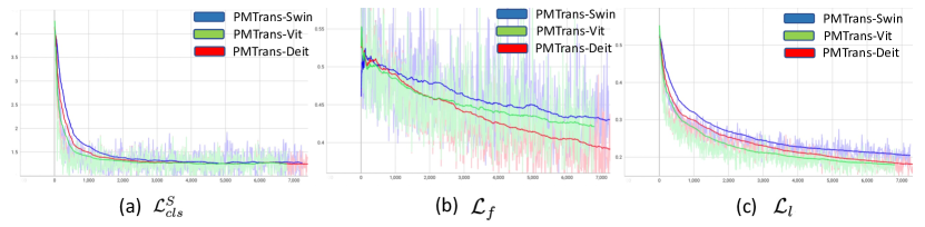
Figure 5: Loss on task A $\to$ C (Office-Home). Lines are smoothed for clarity.

4.3 Testing

In Fig.4, we testify PMTrans-Swin, PMTrans-ViT, and PMTrans-Deit on the task A $\to$ C on the Office-Home dataset. From Fig. 4, with the same number of epochs, PMTrans-ViT achieves faster convergence than PMTrans-Swin and PMTrans-Deit. Besides, the results further reveal that our proposed PMTrans with different transformer backbones can bridge the source and target domains well and decrease domain divergence effectively.

4.4 Complexity

We compare our computational budget with the typical work CDTrans [25] on aligning the source and target domains, excluding the choice of backbone. Precisely, CDTrans compute the similarity between patches from two domains by the multi-head self-attention. We are given $n$ as the sequence length, $d$ as the representation dimension, and $c$ as the number of classes. The per-layer complexity is $O(n^{2}d)$. While in PMTrans, we adopt CE loss to close the domain gap on both the feature and label spaces of the out, whose complexity is $O(d)+O(c)$. When building the intermediate domain, PatchMix samples patches element-wisely, and its complexity is $O(n)$. As attention scores we use are taken directly from the parameters of Transformer and Classifier, so it brings no additional cost. PMTrans’s complexity is $O(d+c+n)$, so it is much more lightweight than the cross attention in CDTrans.

4.5 Attention map visualization for target data

We randomly sample four images from Product (P) of Office-Home and use the pre-trained models $C\to P$ including PMTrans-Swin and PMTrans-Deit to infer the attention maps following the methods described in Sec.2.2. In Fig. 6, we compare the two PMTrans with their counterparts trained with only source classification loss. We observe that after domain alignment, the attention maps tend to be more focused on the objects i.e. less noise around them. Interestingly, for the image whose ground truth label is pencil in the fourth row, Swin-based backbone can distinguish it from plasticine around or attached to it. At the same time, Deit-based attention covers them all, which may bring negative effects. When the attention scores are used to scale the weights of patches during constructing the intermediate domain in Eq.10, Swin-based architecture can focus more on semantics while others may not. That may be one of the reasons why PMTrans-Swin gets superior performance on many datasets. Similarly, TS-CAM [7] names the original attention scores from Transformer like Fig.1 (a) as semantic-agnostic, while what we do in Fig.1 (b) is to reallocate the semantics from Classifier back into the patches and make it be aware of specific class activation.

5 Ablation Study

5.1 Batch size

In Tab. 4, we study the effect of the batch size with different backbones in our proposed PMTrans framework. As shown in Tab. 4, when the batch size is bigger, the input can represent the data distributions better, and therefore the proposed PMTrans based on different backbones with larger batch sizes generally achieves better performance in UDA tasks. Considering the hardware limit, we cannot train models with a batch size of more than 32, so our performance may be lower than it could be, especially when putting in the same condition with a 64 batch size as many previous works do.

5.2 Semi-supervised mixup loss with class information

Tab.  5 shows the comparisons between PMTrans, where the semi-supervised mixup loss combines the class information of target data or not. Note that we use the pseudo labels of target data to calculate the discrepancy between the features and labels. We agree that the semi-supervised mixup loss with class information decreases the domain gaps by reducing the disparity between the feature and label similarities with supervised techniques.

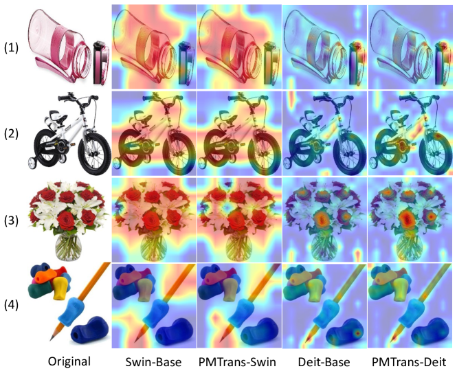
Figure 6: Attention visualization on Swin-based and Deit-based backbones.

6 Discussion and Details

6.1 Details of mixing labels

In practice, labels are weighted by attention score, since attention score of high-response regions accounts for most of the context ( as shown in Fig. 6). Therefore, mixing the re-weight labels approximates mixing labels, which is equivalent to mixing patches proved by Theorem.1. Experiments verify that PMTrans with attention score converges easier without sacrificing performance.

6.2 Details of semi-supervised losses

Pseudo-label generation in the target domain is done by every epoch. As the performance of cross-attention in CDTrans highly depends on the quality of pseudo labels, it becomes less effective when the domain gap becomes large. Therefore, we address this issue in three ways: (a) building the intermediate domain; (b) re-weighting intermediate images’ labels; (c) generating the pseudo labels of the target at each epoch. This way, the pseudo labels of the target are more reliable as the domain shift decreases, thus enabling the proposed PMTrans to transfer the knowledge between domains well.

6.3 Details of $y^{it}$

Note that $y^{it}$ indeed does not cause any confirmation bias because $y^{it}$ is defined without considering pseudo labels of target (as only noisy pseudo labels lead to confirmation bias). The novelty of our idea lies in that we utilize the identity matrix to measure the label similarity $y^{it}$ (without using pseudo labels of target) instead of similarity, like $y^{is}$, to decrease the confirmation bias.

6.4 Learning hyper-parameters of mixup

PatchMix mixes patches from two domains for maximizing CE even if $\lambda$ is fixed. That is, PatchMix can maximize CE, and the other two players minimize CE. More importantly, we propose to learn the parameters of Beta distribution for the flexible or learnable mixup, so as to build a more effective intermediate domain for bridging the source and target domains. Numerically, Tab. 6 in main paper demonstrates that learning parameters of Beta distribution is superior than the fixed parameters in the same min-max CE game.

6.5 t-SNE visualization

Source instances are naturally more cohesive than target instances because only source supervision is accessible before adaptation. After adaptation, PMTrans constructs the compact cluster of the target domain instances closer to the source domain instances than Swin-Base. The comparison of visualization proves that PMTrans can effectively bridge the gap between domains.

6.6 Effectiveness of attention score

We conduct an ablation study on Office-Home; and PMTrans-ViT with or without attention score achieves the same performance 88.9%. And results show PMTrans with attention are easier to converge than that without attention due PMTrans can utilize attention score to obtain high-response regions.

6.7 Impart of patch size on performance

We compare our PMTrans with SSRT using the same batch size as 32 for an apple-to-apple comparison. The result shows that PMTrans achieve comparable performance with SSRT (88.0% vs. 88.0%), demonstrating the effectiveness of PMTrans.

References

- [1] David Acuna, Marc T. Law, Guojun Zhang, and Sanja Fidler. Domain adversarial training: A game perspective. CoRR, abs/2202.05352, 2022.
- [2] Jieneng Chen, Shuyang Sun, Ju He, Philip H. S. Torr, Alan L. Yuille, and Song Bai. Transmix: Attend to mix for vision transformers. CoRR, abs/2111.09833, 2021.
- [3] Shuhao Cui, Shuhui Wang, Junbao Zhuo, Liang Li, Qingming Huang, and Qi Tian. Towards discriminability and diversity: Batch nuclear-norm maximization under label insufficient situations. In 2020 IEEE/CVF Conference on Computer Vision and Pattern Recognition, CVPR 2020, Seattle, WA, USA, June 13-19, 2020, pages 3940–3949. Computer Vision Foundation / IEEE, 2020.
- [4] Terrance Devries and Graham W. Taylor. Improved regularization of convolutional neural networks with cutout. CoRR, abs/1708.04552, 2017.
- [5] Zhekai Du, Jingjing Li, Hongzu Su, Lei Zhu, and Ke Lu. Cross-domain gradient discrepancy minimization for unsupervised domain adaptation. In IEEE Conference on Computer Vision and Pattern Recognition, CVPR 2021, virtual, June 19-25, 2021, pages 3937–3946. Computer Vision Foundation / IEEE, 2021.
- [6] Yaroslav Ganin and Victor S. Lempitsky. Unsupervised domain adaptation by backpropagation. In Proceedings of the 32nd International Conference on Machine Learning, ICML 2015, Lille, France, 6-11 July 2015, volume 37 of JMLR Workshop and Conference Proceedings, pages 1180–1189. JMLR.org, 2015.
- [7] Wei Gao, Fang Wan, Xingjia Pan, Zhiliang Peng, Qi Tian, Zhenjun Han, Bolei Zhou, and Qixiang Ye. TS-CAM: token semantic coupled attention map for weakly supervised object localization. CoRR, abs/2103.14862, 2021.
- [8] Guoliang Kang, Lu Jiang, Yi Yang, and Alexander G. Hauptmann. Contrastive adaptation network for unsupervised domain adaptation. In IEEE Conference on Computer Vision and Pattern Recognition, CVPR 2019, Long Beach, CA, USA, June 16-20, 2019, pages 4893–4902. Computer Vision Foundation / IEEE, 2019.
- [9] Chen-Yu Lee, Tanmay Batra, Mohammad Haris Baig, and Daniel Ulbricht. Sliced wasserstein discrepancy for unsupervised domain adaptation. In IEEE Conference on Computer Vision and Pattern Recognition, CVPR 2019, Long Beach, CA, USA, June 16-20, 2019, pages 10285–10295. Computer Vision Foundation / IEEE, 2019.
- [10] Shuang Li, Mixue Xie, Kaixiong Gong, Chi Harold Liu, Yulin Wang, and Wei Li. Transferable semantic augmentation for domain adaptation. In IEEE Conference on Computer Vision and Pattern Recognition, CVPR 2021, virtual, June 19-25, 2021, pages 11516–11525. Computer Vision Foundation / IEEE, 2021.
- [11] Shuang Li, Mixue Xie, Fangrui Lv, Chi Harold Liu, Jian Liang, Chen Qin, and Wei Li. Semantic concentration for domain adaptation. In 2021 IEEE/CVF International Conference on Computer Vision, ICCV 2021, Montreal, QC, Canada, October 10-17, 2021, pages 9082–9091. IEEE, 2021.
- [12] Ilya Loshchilov and Frank Hutter. Decoupled weight decay regularization. In 7th International Conference on Learning Representations, ICLR 2019, New Orleans, LA, USA, May 6-9, 2019. OpenReview.net, 2019.
- [13] You-Wei Luo and Chuan-Xian Ren. Conditional bures metric for domain adaptation. In IEEE Conference on Computer Vision and Pattern Recognition, CVPR 2021, virtual, June 19-25, 2021, pages 13989–13998. Computer Vision Foundation / IEEE, 2021.
- [14] Jaemin Na, Heechul Jung, Hyung Jin Chang, and Wonjun Hwang. Fixbi: Bridging domain spaces for unsupervised domain adaptation. In IEEE Conference on Computer Vision and Pattern Recognition, CVPR 2021, virtual, June 19-25, 2021, pages 1094–1103. Computer Vision Foundation / IEEE, 2021.
- [15] Xingchao Peng, Qinxun Bai, Xide Xia, Zijun Huang, Kate Saenko, and Bo Wang. Moment matching for multi-source domain adaptation. In 2019 IEEE/CVF International Conference on Computer Vision, ICCV 2019, Seoul, Korea (South), October 27 - November 2, 2019, pages 1406–1415. IEEE, 2019.
- [16] Xingchao Peng, Ben Usman, Neela Kaushik, Judy Hoffman, Dequan Wang, and Kate Saenko. Visda: The visual domain adaptation challenge. CoRR, abs/1710.06924, 2017.
- [17] Kate Saenko, Brian Kulis, Mario Fritz, and Trevor Darrell. Adapting visual category models to new domains. In Computer Vision - ECCV 2010, 11th European Conference on Computer Vision, Heraklion, Crete, Greece, September 5-11, 2010, Proceedings, Part IV, volume 6314 of Lecture Notes in Computer Science, pages 213–226. Springer, 2010.
- [18] Kuniaki Saito, Kohei Watanabe, Yoshitaka Ushiku, and Tatsuya Harada. Maximum classifier discrepancy for unsupervised domain adaptation. In 2018 IEEE Conference on Computer Vision and Pattern Recognition, CVPR 2018, Salt Lake City, UT, USA, June 18-22, 2018, pages 3723–3732. Computer Vision Foundation / IEEE Computer Society, 2018.
- [19] Astuti Sharma, Tarun Kalluri, and Manmohan Chandraker. Instance level affinity-based transfer for unsupervised domain adaptation. In IEEE Conference on Computer Vision and Pattern Recognition, CVPR 2021, virtual, June 19-25, 2021, pages 5361–5371. Computer Vision Foundation / IEEE, 2021.
- [20] Tao Sun, Cheng Lu, Tianshuo Zhang, and Haibin Ling. Safe self-refinement for transformer-based domain adaptation. CoRR, abs/2204.07683, 2022.
- [21] Korawat Tanwisuth, Xinjie Fan, Huangjie Zheng, Shujian Zhang, Hao Zhang, Bo Chen, and Mingyuan Zhou. A prototype-oriented framework for unsupervised domain adaptation. In Advances in Neural Information Processing Systems 34: Annual Conference on Neural Information Processing Systems 2021, NeurIPS 2021, December 6-14, 2021, virtual, pages 17194–17208, 2021.
- [22] Hemanth Venkateswara, Jose Eusebio, Shayok Chakraborty, and Sethuraman Panchanathan. Deep hashing network for unsupervised domain adaptation. In 2017 IEEE Conference on Computer Vision and Pattern Recognition, CVPR 2017, Honolulu, HI, USA, July 21-26, 2017, pages 5385–5394. IEEE Computer Society, 2017.
- [23] Vikas Verma, Alex Lamb, Christopher Beckham, Amir Najafi, Ioannis Mitliagkas, David Lopez-Paz, and Yoshua Bengio. Manifold mixup: Better representations by interpolating hidden states. In Proceedings of the 36th International Conference on Machine Learning, ICML 2019, 9-15 June 2019, Long Beach, California, USA, volume 97 of Proceedings of Machine Learning Research, pages 6438–6447. PMLR, 2019.
- [24] Ni Xiao and Lei Zhang. Dynamic weighted learning for unsupervised domain adaptation. In IEEE Conference on Computer Vision and Pattern Recognition, CVPR 2021, virtual, June 19-25, 2021, pages 15242–15251. Computer Vision Foundation / IEEE, 2021.
- [25] Tongkun Xu, Weihua Chen, Pichao Wang, Fan Wang, Hao Li, and Rong Jin. Cdtrans: Cross-domain transformer for unsupervised domain adaptation. CoRR, abs/2109.06165, 2021.
- [26] Jinyu Yang, Jingjing Liu, Ning Xu, and Junzhou Huang. TVT: transferable vision transformer for unsupervised domain adaptation. CoRR, abs/2108.05988, 2021.
- [27] Sangdoo Yun, Dongyoon Han, Sanghyuk Chun, Seong Joon Oh, Youngjoon Yoo, and Junsuk Choe. Cutmix: Regularization strategy to train strong classifiers with localizable features. In 2019 IEEE/CVF International Conference on Computer Vision, ICCV 2019, Seoul, Korea (South), October 27 - November 2, 2019, pages 6022–6031. IEEE, 2019.
- [28] Hongyi Zhang, Moustapha Cissé, Yann N. Dauphin, and David Lopez-Paz. mixup: Beyond empirical risk minimization. In 6th International Conference on Learning Representations, ICLR 2018, Vancouver, BC, Canada, April 30 - May 3, 2018, Conference Track Proceedings. OpenReview.net, 2018.
- [29] Yuchen Zhang, Tianle Liu, Mingsheng Long, and Michael I. Jordan. Bridging theory and algorithm for domain adaptation. In Proceedings of the 36th International Conference on Machine Learning, ICML 2019, 9-15 June 2019, Long Beach, California, USA, volume 97 of Proceedings of Machine Learning Research, pages 7404–7413. PMLR, 2019.
- [30] Yabin Zhang, Hui Tang, Kui Jia, and Mingkui Tan. Domain-symmetric networks for adversarial domain adaptation. In IEEE Conference on Computer Vision and Pattern Recognition, CVPR 2019, Long Beach, CA, USA, June 16-20, 2019, pages 5031–5040. Computer Vision Foundation / IEEE, 2019.
- [31] Bolei Zhou, Aditya Khosla, Àgata Lapedriza, Aude Oliva, and Antonio Torralba. Learning deep features for discriminative localization. CoRR, abs/1512.04150, 2015.