Interacting Particle Langevin Algorithm for Maximum Marginal Likelihood Estimation

Abstract

We develop a class of interacting particle systems for implementing a maximum marginal likelihood estimation (MMLE) procedure to estimate the parameters of a latent variable model. We achieve this by formulating a continuous-time interacting particle system which can be seen as a Langevin diffusion over an extended state space of parameters and latent variables. In particular, we prove that the parameter marginal of the stationary measure of this diffusion has the form of a Gibbs measure where number of particles acts as the inverse temperature parameter in classical settings for global optimisation. Using a particular rescaling, we then prove geometric ergodicity of this system and bound the discretisation error in a manner that is uniform in time and does not increase with the number of particles. The discretisation results in an algorithm, termed Interacting Particle Langevin Algorithm (IPLA) which can be used for MMLE. We further prove nonasymptotic bounds for the optimisation error of our estimator in terms of key parameters of the problem, and also extend this result to the case of stochastic gradients covering practical scenarios. We provide numerical experiments to illustrate the empirical behaviour of our algorithm in the context of logistic regression with verifiable assumptions. Our setting provides a straightforward way to implement a diffusion-based optimisation routine compared to more classical approaches such as the Expectation Maximisation (EM) algorithm, and allows for especially explicit nonasymptotic bounds.

1 Introduction

Parameter estimation in the presence of hidden, latent, or unobserved variables is key in modern statistical practice. This setting arises in multiple applications such as frequentist inference (Casella and Berger, 2021), empirical Bayes (Carlin and Louis, 2000) and most notably latent variable models to model complex datasets such as images (Bishop, 2006), text (Blei et al., 2003), audio (Smaragdis et al., 2006), and graphs (Hoff et al., 2002). Latent variable models (LVMs) allow us to handle complex datasets by decomposing them into a set of trainable parameters and a set of latent variables which correspond to the underlying structure of the data. However, learning models with hidden, unobserved, or latent variables is challenging as, in order to find a maximum likelihood estimate (MLE), we first need to tackle an intractable integral.

Broadly speaking, the problem of parameter inference in models with latent variables can be formalized as a maximum marginal likelihood estimation problem (Dempster et al., 1977). In this setting, there are three main ingredients of the probabilistic model: The parameters, the latent variables, and the observed data. More precisely, in maximum marginal likelihood estimation we consider a probabilistic model with observed data $y$ and likelihood $p_{\theta}(x,y)$ parametrised by $\theta\in{}^{d_{\theta}}$, where $x\in{}^{d_{x}}$ is a latent variable which cannot be observed. Our aim is to find $\bar{\theta}^{\star}$ maximising the marginal likelihood $p_{\theta}(y):=\int_{{}^{d_{x}}}p_{\theta}(x,y)\mathrm{d}x$. In the literature, the standard way to solve maximum marginal likelihood estimation problems is to use the Expectation Maximisation (EM) algorithm (Dempster et al., 1977), an iterative procedure which is guarantee to converge to a (potentially local) maximiser of $p_{\theta}(y)$. The EM algorithm consists of two steps, where the first step is an expectation step (E-step) w.r.t. the latent variables while the second step is a maximisation step (M-step) w.r.t. the parameters. While initially this algorithm was mainly implemented in the case where both steps are exact, it has been shown that the EM algorithm can be implemented with approximate steps, e.g., using Monte Carlo methods for the E-step (Wei and Tanner, 1990, Sherman et al., 1999), approximating the expectation step. Similarly, the M-step can be approximated using numerical optimisation algorithms (Meng and Rubin, 1993, Liu and Rubin, 1994), e.g., gradient descent (Lange, 1995). The ubiquity of latent variable models and the effectiveness of the EM algorithm compared to its alternatives has led to a flurry of research in the last decades for its approximate implementation. In particular, a class of algorithms called Monte Carlo EM (MCEM; Wei and Tanner (1990)) or stochastic EM (SEM; Celeux (1985)) algorithms have been extensively analysed and used in the literature, see, e.g., Celeux and Diebolt (1992), Chan and Ledolter (1995), Sherman et al. (1999), Booth and Hobert (1999), Cappé et al. (1999), Diebolt and Ip (1996). This method replaces the E-step with Monte Carlo integration. However, since the expectation in the E-step is w.r.t. the posterior distribution of the latent variables given data, the perfect Monte Carlo integration is often intractable. As a result, a plethora of approximations using Markov chain Monte Carlo (MCMC) for the E-step have been proposed and the convergence properties of the resulting algorithms have been studied, see, e.g., Delyon et al. (1999), Fort et al. (2011), Fort and Moulines (2003), Caffo et al. (2005), Atchadé et al. (2017). Standard Markov chain Monte Carlo (MCMC) methods, however, may be hard to implement and slow to converge, particularly when the dimension of the latent variables is high. This is due to the fact that standard MCMC (Metropolis-based) kernels may be hard to calibrate and may get stuck in local modes easily. To alleviate such problems, a number of unadjusted Markov chain Monte Carlo methods have been proposed, most notably, the unadjusted Langevin algorithm (ULA) (Durmus and Moulines, 2017, Dalalyan, 2017a, b) based on Langevin diffusions (Roberts and Tweedie, 1996). These approaches are based on a simple discretisation of the Langevin stochastic differential equation (SDE) and have become a popular choice for MCMC methods in high dimensional setting with favourable theoretical properties, see, e.g., Durmus and Moulines (2019), Vempala and Wibisono (2019), Durmus et al. (2019), Brosse et al. (2019), Dalalyan and Karagulyan (2019), Chewi et al. (2022) and references therein.

Naturally, MCMC methods based on unadjusted Markov kernels like ULA have been also used in the context of EM. In particular, De Bortoli et al. (2021) studied the SOUL algorithm which uses ULA (or, more generally, inexact Markov kernels) in order to draw (approximate) samples from the posterior distribution of the latent variables and approximate the E-step. This algorithm proceeds in a coordinate-wise manner, first running a sequence of ULA steps to obtain samples, then approximating the E-step with these samples, and finally moving to the M-step. The convergence analysis has been done under convexity and mixing assumptions but the proofs are based on a particular selection of step-sizes which obfuscates the general applicability of the results. More recently, Kuntz et al. (2023) showed that interacting Langevin dynamics can substantially improve the performance. In particular, Kuntz et al. (2023) used an interacting particle system to approximate the E-step, rather than running a ULA chain. This approach has significantly improved empirical results, however, Kuntz et al. (2023) provided a limited theoretical analysis, in particular, precise nonasymptotic bounds on the convergence rate of the algorithm were not provided.

Looking at marginal maximum likelihood estimation from an optimisation point of view, Gaetan and Yao (2003), Jacquier et al. (2007), Johansen et al. (2008) propose strategies based on simulated annealing to approximate $\bar{\theta}^{\star}$. In particular, Johansen et al. (2008), Duan et al. (2017) consider interacting particle methods based on sequential Monte Carlo.

In the optimisation literature algorithms based on interacting particle systems are often used in place of gradient based methods (e.g. Pinnau et al. (2017), Kennedy and Eberhart (1995), Totzeck and Wolfram (2020), Akyildiz et al. (2020), see also Grassi and Pareschi (2021) for a recent review) or to speed up convergence in gradient-based methods (e.g. Borovykh et al. (2021)). However, to the best of our knowledge, the use of interacting particle systems combined with Langevin dynamics in the context of maximum likelihood estimation has not been widely explored, except for the recent developments in Kuntz et al. (2023) which paved the way for the present work.

Contributions. In this paper, we propose and analyse a new algorithm for maximum marginal likelihood estimation in the context of latent variable models. Our algorithm forms an interacting particle system (IPS) which is based on a time discretisation of a continuous time IPS to approximate the maximum marginal likelihood estimator for models with incomplete or hidden data. Our method uses a similar continuous time system to that of Kuntz et al. (2023) but with a crucial difference in the parameter $(\theta)$ dimension. Specifically, similar to Kuntz et al. (2023), our IPS model is defined over a set of particles $\{X_{1},\ldots,X_{N}\}$, where $X_{i}\in{}^{d_{x}}$, and a parameter $\theta\in{}^{d_{\theta}}$. However, we inject noise into the dynamics of $\theta$, hence obtain an SDE for $\theta$ rather than a deterministic ordinary differential equation (ODE). This allows us to obtain a system with the invariant measure of the form

$$\pi^{N}_{\star}(\theta,x_{1},...,x_{N})\propto e^{-\sum_{i=1}^{N}U(\theta,x_{i})}$$ (1)

where $U(\theta,x):=-\log p_{\theta}(x,y)$ with fixed data $y$. We prove that the $\theta$-marginal of this density concentrates around $\bar{\theta}^{\star}$ as $N\to\infty$ allowing us to obtain nonasymptotic results for the algorithm. It follows that any method of sampling from $\pi^{N}_{\star}$ (keeping only the $\theta$-component) will be a method for maximum-marginal likelihood estimation.

Our approach leverages the rich connection between Langevin dynamics and optimisation (see, e.g., Dalalyan (2017a), Raginsky et al. (2017), Zhang et al. (2023)) and opens up further avenues for proving new results. Using a particular natural rescaling, we are additionally able to prove ergodic bounds and numerical error bounds that are completely independent of the parameter $N$. As the first nonasymptotic results under the interacting setting, our results are obtained in the case where $U$ is gradient Lipschitz and obeys a strong convexity condition, but we believe that similar results can be obtained under much weaker (nonconvex) conditions (Zhang et al., 2023). In this setting the addition of noise into the theta component will be crucial, however we leave this direction for future work.

The remainder of this paper is organized as follows. In Section 2, we set up our framework and summarize the key contributions, the proposed particle system and resulting algorithm, and explain in detail the intuition for our main result. In Section 3, we prove our results with full proofs and provide global error bounds. Proofs of a technical nature will be postponed to Appendix A–C. We supply this section by reviewing closely related work in Section 5, making our contributions and main ideas clearer. We then provide in Section 6 an example on logistic regression where we show our results are applicable to this case. Finally, we conclude in Section 7.

1.1 Notation

We endow ^d with the Borel $\sigma$-field $\mathcal{B}({}^{d})$ with respect to the Euclidean norm $\|\cdot\|$. For $\alpha\in\mathbb{N}\cup\{\infty\}$ we let $C^{\alpha}(\mathbb{R}^{d})$ denote the space of $\alpha$-times differentiable functions on $\mathbb{R}^{d}$, and let $C_{c}^{\alpha}(\mathbb{R}^{d})\subset C^{\alpha}(\mathbb{R}^{d})$ the subspace of $C^{\alpha}(\mathbb{R}^{d})$ consisting of functions with compact support. For all continuously differentiable functions $f$, we denote by $\nabla f$ the gradient. Furthermore, if $f$ is twice continuously differentiable we denote by $\nabla^{2}f$ its Hessian and by $\Delta f$ its Laplacian. For any $p\in\mathbb{N}$ we denote by $\mathcal{P}_{p}({}^{d})=\{\pi\in\mathcal{P}({}^{d}):\int_{{}^{d}}\|x\|_{p}^{p}\mathrm{d}\pi(x)<+\infty\}$ the set of probability measures over $\mathcal{B}({}^{d})$ with finite $p$-th moment. For ease of notation, we define $\mathcal{P}({}^{d})=\mathcal{P}_{0}({}^{d})$ the set of probability measures over $\mathcal{B}({}^{d})$ and endow this space with the topology of weak convergence. For any $\mu,\nu\in\mathcal{P}_{p}({}^{d})$ we define the $p$-Wasserstein distance $W_{p}(\mu,\nu)$ between $\mu$ and $\nu$ by

$$W_{p}(\mu,\nu)=\left(\inf_{\gamma\in\mathbf{T}(\mu,\nu)}\int_{{}^{d}\times{}^{d}}\|x-y\|_{p}^{p}\mathrm{d}\gamma(x,y)\right)^{1/p}$$

where $\mathbf{T}(\mu,\nu)=\{\gamma\in\mathcal{P}({}^{d}\times{}^{d}):\gamma(A\times{}^{d})=\mu(A),\ \gamma({}^{d}\times A)=\nu(A)\ \forall A\in\mathcal{B}({}^{d})\}$ denotes the set of all transport plans between $\mu$ and $\nu$. In the following, we metrise $\mathcal{P}_{p}({}^{d})$ with $W_{p}$.

In the following we adopt the convention that continuous time processes are denoted by bold letters while their time discretisations are not.

2 Background and main results

In this section, we introduce the problem and technical background of relevant work.

2.1 Maximum marginal likelihood estimation and the EM algorithm

In this section, we introduce the problem of maximum marginal likelihood estimation in models with latent, hidden, or unobserved variables.

Let $p_{\theta}(x,\cdot)$ be a joint probability density function of the latent variable $x$ and fixed observed data. We define the negative log-likelihood as

$$U(\theta,x):=-\log p_{\theta}(x,y)$$

for any fixed $y\in{}^{d_{y}}$. The goal of maximum marginal likelihood estimation (MMLE) is to find the parameter $\bar{\theta}^{\star}$ that maximises the marginal likelihood (Dempster et al., 1977)

$$k(\theta):=p_{\theta}(y)=\int p_{\theta}(x,y)\mathrm{d}x=\int e^{-U(\theta,x)}\mathrm{d}x,$$ (2)

where $y\in{}^{d_{y}}$ is the observed (fixed) data. Here $p_{\theta}(y)$ can be interpreted as a function of $\theta$ for fixed observation $y$ as standard in Bayesian literature. Therefore, the problem of maximum marginal likelihood estimation can be seen as maximisation of an intractable integral (2).

2.2 A Particle Langevin SDE and its discretisation

While optimising a function in a standard setup can be done with standard stochastic optimisation techniques in the convex case or with Langevin diffusions in the nonconvex case (Zhang et al., 2023), when the function to be optimised is an intractable integral as in (2), the problem becomes highly non-trivial. This stems from the fact that any gradient estimate w.r.t. $\theta$ will require sampling $x$ variables to estimate the integral. But since sampling from the unnormalised measure $e^{-U(\theta,x)}$ for fixed $\theta$ in this setting is typically intractable, the samples drawn using numerical schemes would be approximate which would incur bias on the gradient estimates. This is the precise problem investigated in prior works, see, e.g., Atchadé et al. (2017) or De Bortoli et al. (2021) for using MCMC chains to sample from $e^{-U(\theta,x)}$ with fixed $\theta$ and use these samples to estimate the gradient of $k(\theta)$. This approach requires non-trivial assumptions on step-sizes of optimisation schemes and sometimes not even computationally tractable as the sample sizes used to estimate gradients may need to increase over iterations.

A different approach was considered in Kuntz et al. (2023) which used a particle system. In other words, at iteration $n$, Kuntz et al. (2023) proposed to use $N$ particles $X^{i,N}_{n}$ to estimate the gradient of $k(\theta)$ which is then minimised using a gradient step. Inspired by this approach, in this work, we propose an interacting Langevin SDE

$$\mathrm{d}\bm{\theta}^{N}_{t} =-\frac{1}{N}\sum_{j=1}^{N}\nabla_{\theta}U(\bm{\theta}^{N}_{t},\bm{X}_{t}^{j,N})\mathrm{d}t+\sqrt{\frac{2}{N}}\mathrm{d}\bm{B}_{t}^{0,N},$$ (3)

$$\mathrm{d}\bm{X}_{t}^{i,N} =-\nabla_{x}U(\bm{\theta}^{N}_{t},\bm{X}_{t}^{i,N})\mathrm{d}t+\sqrt{2}\mathrm{d}\bm{B}_{t}^{i,N},$$ (4)

for $i=1,\dots,N$, where $\{(\bm{B}_{t}^{i,N})_{t\geq 0}\}_{i=0}^{N}$ is a family of independent Brownian motions. This interacting particle system (IPS) is closely related to the one introduced in Kuntz et al. (2023), with one major difference in Eq. (3) where we add the noise term $\sqrt{2/N}\mathrm{d}\bm{B}_{t}^{0,N}$. Despite seemingly small, the addition of the noise term in the $\theta$-component unlocks the way for proving precise nonasymptotic results as we will summarise in Section 2.3 after introducing our algorithm.

The IPS given in Eqs. (3)–(4) can be discretised in a number of ways. In this work, we consider a simple Euler-Maruyama discretisation. This can be defined, given $(\theta_{0},X_{0}^{1:N})\in{}^{d_{\theta}}\times({}^{d})^{\otimes N}$ and for any $n\in\mathbb{N}$, as

$$\theta_{n+1} =\theta_{n}-\frac{\gamma}{N}\sum_{j=1}^{N}\nabla_{\theta}U(\theta_{n},X_{n}^{j,N})+\sqrt{\frac{2\gamma}{N}}\xi_{n+1}^{0,N},$$ (5)

$$X_{n+1}^{i,N} =X_{n}^{i,N}-\gamma\nabla_{x}U(\theta_{n},X_{n}^{i,N})+\sqrt{2\gamma}\xi_{n+1}^{i,N},$$ (6)

where $\gamma>0$ is a time discretisation parameter and $\xi_{n}^{i,N}:=\bm{B}^{i,N}_{n\gamma}-\bm{B}^{i,N}_{(n-1)\gamma}$ are iid standard Gaussians for $i=0,\dots,N$. Algorithm 1 summarises our method to approximate $\bar{\theta}^{\star}$. We call our resulting method Interacting Particle Langevin Algorithm (IPLA).

As in the case of our IPS, this algorithm is similar to the one proposed in Kuntz et al. (2023) (see Algorithm 1 therein) but with the crucial difference that we inject noise in the $\theta$-direction as well. This seemingly small algorithmic difference enables us to obtain a number of results about the invariant measure of the corresponding continuous-time IPS and the nonasymptotic convergence of the algorithm to the optimal solution. For future work, we imagine that the addition of noise will allow for our algorithm to be especially effective in the nonconvex case, since this will allow the theta component to escape more easily from shallow local minima. Furthermore, this method could be adapted to an effective annealing algorithm, where more particles are introduced as a function of time. However for the present work we consider the simplest possible case.

Algorithm 1 Interacting Particle Langevin Algorithm (IPLA)

  Require: $N,\gamma,\pi_{\mathrm{init}}\in{\mathcal{P}}({}^{d_{\theta}})\times{\mathcal{P}}(({}^{d})^{N})$

  Draw $(\theta_{0},\{X_{0}^{i,N}\}_{i=1}^{N})$ from $\pi_{\mathrm{init}}$

  for $n=1:n_{T}$ do

     $\theta_{n+1}=\theta_{n}-\frac{\gamma}{N}\sum_{j=1}^{N}\nabla_{\theta}U(\theta_{n},X_{n}^{j,N})+\sqrt{\frac{2\gamma}{N}}\xi_{n+1}^{0,N}$ and $X_{n+1}^{i,N}=X_{n}^{i,N}-\gamma\nabla_{x}U(\theta_{n},X_{n}^{i,N})+\sqrt{2\gamma}\xi_{n+1}^{i,N}$

  end for

  return  $\theta_{n_{T}+1}$

2.3 The proof plan and the main result

In this section, we summarise the main ideas behind our analysis of the scheme given in (5)–(6) and our final result which quantifies the convergence of the sequence $(\theta_{n})_{n\geq 1}$ to the minimiser of $k$, namely $\bar{\theta}^{\star}$. A standard result from the literature shows that finding minimisers of $k$ also solves the problem of sampling from the posterior distribution $p_{\bar{\theta}^{\star}}(x|y)$, see, e.g., Neal and Hinton (1998) or Kuntz et al. (2023, Theorem 1).

In what follows, we will sketch our results on the invariant measure, the convergence of the IPS (3)–(4) and the discrete algorithm (5)–(6). These results will extend proofs from a standard Langevin diffusion to the much more complicated particle systems we consider. A key aspect of our theoretical framework is that we consider the rescaled version of our particle system given as

$$\bm{Z}_{t}^{N}=(\bm{\theta}^{N}_{t},N^{-1/2}\bm{X}_{t}^{1,N},\ldots,N^{-1/2}\bm{X}_{t}^{N,N}).$$ (7)

which proves much easier to analyse, and causes no loss in precision since we shall be considering only the convergence of the $\theta_{n}$ component.

Our proof can be summarised in a few main steps we describe below.

2.3.1 Invariant measure

After showing that the IPS has a strong unique solution in Prop. 1, our first result (in Prop. 2) shows that, as mentioned in the Introduction, the IPS (3)–(4) leaves

$$\pi^{N}_{\star}(\theta,x_{1},...,x_{N})\propto e^{-\sum_{i=1}^{N}U(\theta,x_{i})}$$

invariant. This is a crucial result as this measure has concentration properties that will be very useful in the next section.

2.3.2 Concentration of the invariant measure around the minimiser

The usefulness of proving results in Section 2.3.1 becomes apparent in our setup with the crucial observation that the $\theta$-marginal of $\pi_{\star}^{N}$ concentrates around $\bar{\theta}^{\star}\in\arg\max_{\theta\in{\mathbb{R}}^{d_{\theta}}}k(\theta)$.

To show this, we denote the $\theta$-marginal of $\pi_{\star}^{N}$ as $\pi_{\Theta}^{N}$ and we prove (in Prop. 3) that under strong convexity assumptions (see Section 3)

$$W_{2}(\pi^{N}_{\Theta},\delta_{\bar{\theta}^{\star}})\leq\sqrt{\frac{2d_{\theta}}{\mu N}},$$

where $\mu$ is related to the convexity properties assumed, i.e., the $\theta$-marginal concentrates around the Dirac measure located at the maximiser $\bar{\theta}^{\star}$. This allows us to derive optimisation errors in our final result.

2.3.3 Convergence rate of the IPS (3)–(4)

Our next result shows that, not only $\pi_{\star}^{N}$ is the invariant measure, but under appropriate smoothness and convexity assumptions which will be made clear in Section 3, we show (in Prop. 4) that under appropriate conditions on the initial condition, we have

$$W_{2}(\mathcal{L}_{\theta_{0}}(\bm{\theta}^{N}_{t}),\pi_{\Theta}^{N})\leq e^{-\mu t}\left(C_{0}+\frac{d_{x}N+d_{\theta}}{N\mu}\right)^{1/2},$$

where $\mu$ is related to the convexity properties assumed, $C_{0}<\infty$ is the initialisation error (see Prop. 4 for its precise form) and ${\mathcal{L}}_{\theta_{0}}(\bm{\theta}^{N}_{t})$ is the $\theta$-marginal of the measure associated to the law of the IPS (3)–(4) at time $t$. Prop. 4 in particular is akin to the standard results on Langevin diffusions (Durmus and Moulines, 2017, 2019), but, due to the presence of the particle system the same technique cannot be applied straightforwardly and the rescaling (7) becomes necessary.

2.3.4 Discretisation analysis

While above results prove that the law of the IPS SDE in (3)–(4) would concentrate around the minimiser in $\theta$ marginal, we still have to handle the discretisation error of the algorithm (5)–(6). One expects dimensional scaling of order at least $O(d^{1/2})$ for the Wasserstein-$2$ numerical error of Langevin type algorithms (see Durmus and Moulines (2019)), in which case one would expect the numerical error for (5)–(6) to scale badly with the number of particles. However, by considering only the error in the $\Theta$-marginal and using the rescaling (7), we prove that the numerical error does not worsen as $N$ increases. In particular, we prove in Prop. 5 that

$$W_{2}(\mathcal{L}(\theta_{n}),\mathcal{L}(\bm{\theta}^{N}_{n\gamma}))\leq C_{1}(1+\sqrt{d_{\theta}/N+d_{x}})\gamma^{1/2},$$

where $\gamma$ is the step-size given in (5)–(6) and $C_{1}>0$ is a constant independent of $N,d_{\theta},d_{x},\gamma,n$. Additionally, under further smoothness assumptions for $\nabla U$ we prove that

$$W_{2}(\mathcal{L}(\theta_{n}),\mathcal{L}(\bm{\theta}^{N}_{n\gamma}))\leq C_{2}(1+d_{\theta}/N+d_{x})\gamma.$$

(for a constant $C_{2}>0$ also independent of $N,d_{\theta},d_{x},\gamma,n$). This proves that the law of the algorithm (5)–(6) stays close to the law of the SDE (3)–(4) in an appropriate sense.

2.3.5 The main result

Recall that our main aim is to show that the sequence $(\theta_{n})_{n\geq 1}$ optimises $k(\theta)$, in other words $\theta_{n}$ converges to $\bar{\theta}^{\star}$ (which is unique under our strong convexity assumptions; see Section 3). Using the triangle inequality we obtain the following splitting of the optimisation error into three terms

$$\mathbb{E}\left[\|\theta_{n}-\bar{\theta}^{\star}\|^{2}\right]^{1/2} =W_{2}(\delta_{\bar{\theta}^{\star}},\mathcal{L}(\theta_{n}))$$

$$\leq W_{2}(\delta_{\bar{\theta}^{\star}},\pi^{N}_{\Theta})+W_{2}(\pi^{N}_{\Theta},\mathcal{L}(\bm{\theta}^{N}_{n\gamma}))+W_{2}(\mathcal{L}(\bm{\theta}^{N}_{n\gamma}),\mathcal{L}_{\theta_{0}}(\theta_{n})),$$

where each term can be bounded using the results described in the previous sections.

We prove in Theorem 1 that $\theta$-iterates in Algorithm 1 satisfy the following nonasymptotic convergence result

$$\mathbb{E}\left[\|\theta_{n}-\bar{\theta}^{\star}\|^{2}\right]^{1/2}\leq\sqrt{\frac{d_{\theta}}{N\mu}}+e^{-\mu n\gamma}\left(C_{0}+\left(\frac{d_{x}N+d_{\theta}}{N\mu}\right)^{1/2}\right)+C_{1}(1+\sqrt{d_{\theta}/N+d_{x}})\gamma^{1/2},$$

where $\mu$ is related to the convexity properties that we assume (see Section 3), $\gamma$ is the time discretisation parameter, $N$ is the number of particles, and $C_{1}$ is a constant independent of $N,n,d_{\theta},d_{x},\gamma$ defined for $\gamma$ sufficiently small. Furthermore, under the additional smoothness assumption A 4 one has the following error with improved order of numerical convergence

$$\mathbb{E}\left[\|\theta_{n}-\bar{\theta}^{\star}\|^{2}\right]^{1/2}\leq\sqrt{\frac{d_{\theta}}{N\mu}}+e^{-\mu n\gamma}\left(C_{0}+\left(\frac{d_{x}N+d_{\theta}}{N\mu}\right)^{1/2}\right)+C_{2}(1+d_{\theta}/N+d_{x})\gamma,$$

This result is the first of its kind for the IPS based methods for the MMLE problem.

3 Analysis

As mentioned above, the results we would like to achieve require smoothness and convexity assumptions on $U$ which we now summarise. We first provide essential assumptions that will be central for our main results. We will also introduce further smoothness assumption to refine these results a bit later.

First, we assume that $\nabla U(\theta,x)$ is Lipschitz in both variables.

A 1.

Let $v=(\theta,x)$ and $v^{\prime}=(\theta^{\prime},x^{\prime})$. We assume that $U\in C^{1}(\mathbb{R}^{d_{\theta}+d_{x}})$ and that there exists $L>0$ such that

$$\|\nabla U(v)-\nabla U(v^{\prime})\|\leq L\|v-v^{\prime}\|.$$

We also assume that the following strong convexity condition holds.

A 2.

Let $v=(\theta,x)$. Then, there exists $\mu>0$ such that

$$\left\langle v-v^{\prime},\nabla U(v)-\nabla U(v^{\prime})\right\rangle\geq\mu\|v-v^{\prime}\|^{2},$$

for all $v,v^{\prime}\in{}^{d_{\theta}}\times{}^{d_{x}}$.

A 3.

There is a constant $H>0$ such that the initial condition $Z^{N}_{0}=(\theta_{0},N^{-1/2}X^{1,N}_{0},...,N^{-1/2}X^{N,N}_{0})$ satisfies ${\mathbb{E}}[\|Z^{N}_{0}\|^{2}]\leq H$.

A 1 is common in the literature on interacting particle systems and guarantees that both the interacting particle system (3)–(4) and its time discretisation (5)–(6) are stable (see, e.g., Sznitman (1991), Bossy and Talay (1997)). A 2 guarantees that $U$ has a unique minimiser $v^{\star}=(\theta^{\star},x^{\star})$, and A 3 ensures that the continuous time and discretised processes both have finite second moment for all time.

Remark 1.

We note that the strong monotonicity assumption A 2 on $\nabla U$ is equivalent to the assertion that $U$ is strongly convex, which in turns implies a quadratic lower bound on the growth of $U$. Therefore $e^{-U}$ is absolutely integrable, and so the Leibniz integral rule for differentiation under the integral sign (e.g. Billingsley (1995, Theorem 16.8)) guarantees that

$$\nabla k(\theta)=\nabla\int_{{}^{d_{x}}}e^{-U(\theta,x)}\mathrm{d}x=-\int_{{}^{d_{x}}}\nabla_{\theta}U(\theta,x)e^{-U(\theta,x)}\mathrm{d}x.$$ (8)

3.1 Continuous-time process and its invariant measure

Recall our continuous-time interacting SDE introduced in Eqs. (3)–(4)

$$\mathrm{d}\bm{\theta}^{N}_{t}=-\frac{1}{N}\sum_{j=1}^{N}\nabla_{\theta}U(\bm{\theta}^{N}_{t},\bm{X}_{t}^{j,N})\mathrm{d}t+\sqrt{\frac{2}{N}}\mathrm{d}\bm{B}_{t}^{0,N},\qquad\mathrm{d}\bm{X}_{t}^{i,N}=-\nabla_{x}U(\bm{\theta}^{N}_{t},\bm{X}_{t}^{i,N})\mathrm{d}t+\sqrt{2}\mathrm{d}\bm{B}_{t}^{i,N},$$ (9)

In what follows, we show that (9) admits a unique solution under A 1.

Proposition 1.

Let A 1 and A 3 hold. Then there exist a unique strong solution to (9).

Proof.

We can consider the system (9) as one SDE defined over ^d with $d=d_{\theta}+Nd_{x}$. The drift coefficient of this SDE is given by $b:\mathbb{R}^{d}\to\mathbb{R}^{d}$ with

$$b(\theta,x_{1},\dots,x_{N}):=(-N^{-1}\sum_{j=1}^{N}\nabla_{\theta}U(\theta,x_{j}),-\nabla_{x}U(\theta,x_{1}).\dots,-\nabla_{x}U(\theta,x_{N})),$$ (10)

and constant diffusion coefficient. Under A 1, it is easy to show that $b$ is Lipschitz continuous w.r.t. $\theta$ and $x_{1},\dots,x_{N}$ and thus locally bounded, this and A 3 ensure that there exist a unique strong solution to (9) (see, for instance, Karatzas and Shreve (1991, Chapter 5, Theorem 2.9)). ∎

Having shown that (9) admits a unique solution, we now investigate its invariant measure.

Proposition 2 (Invariant measure).

For any $N\in\mathbb{N}$, the measure $\pi_{\star}^{N}(\theta,x_{1},...,x_{N})\propto e^{-\sum^{N}_{i=1}U(\theta,x_{i})}$ is an invariant measure for the IPS (9).

Proof.

Recall that for a $\mathbb{R}^{d}$-valued SDE with drift $b:\mathbb{R}^{d}\to\mathbb{R}^{d}$ and diffusion coefficient $\sigma:\mathbb{R}^{d}\to\mathbb{R}^{d\times d}$, the ‘infinitesimal generator’ $\mathcal{L}$ is the operator on $C^{2}(\mathbb{R}^{d})$ given as

$$\mathcal{L}=\langle b,\nabla\rangle+\frac{1}{2}\sigma\sigma^{T}:\nabla^{2},$$

where $:$ denotes the Frobenius inner product and where one adopts the standard abuse of notation that treats operators like tensors, so that the first term for instance corresponds to the operator $\sum_{i=1}^{d}b_{i}\partial_{x_{i}}$. One has by Lelièvre and Stoltz (2016, 1.17, page 696) that a probability measure $\pi$ on $\mathbb{R}^{d}$ is an invariant measure for the process with generator $\mathcal{L}$ if for any $\varphi\in C^{\infty}_{c}(\mathbb{R}^{d})$ one has

$$\int_{\mathbb{R}^{d}}\mathcal{L}\varphi\;{\mathrm{d}}\pi=0.$$

Now let us consider (9) as one SDE on $\mathbb{R}^{d_{\theta}+Nd_{x}}$ with generator $\mathcal{L}$. Then, for every $\varphi\in C^{\infty}_{c}(\mathbb{R}^{d_{\theta}+Nd_{x}})$ one has

$$\mathcal{L}\varphi =-N^{-1}\sum_{j=1}^{N}\langle\nabla_{\theta}U(\theta,x_{j}),\nabla_{\theta}\varphi\rangle-\sum_{j=1}^{N}\langle\nabla_{x}U(\theta,x_{j}),\nabla_{x_{j}}\varphi\rangle+N^{-1}\Delta_{\theta}\varphi+\sum_{j=1}^{N}\Delta_{x_{j}}\varphi.$$

Let $\rho:\mathbb{R}^{d_{\theta}+Nd_{x}}\to\mathbb{R}$ denote the density of $\pi^{N}_{\star}$, so that $\rho(\theta,{\mathbf{x}}_{1},...,x_{N})=ce^{-\sum^{N}_{i=1}U(\theta,x_{i})}$ for some $c>0$, and observe that therefore by A 1 one has $\rho\in C^{1}(\mathbb{R}^{d_{\theta}+Nd_{x}})$. Now let us denote by $\operatorname{div}_{\theta}$ the divergence of a function as a function of $\theta$ alone, so that $\operatorname{div}_{\theta}(\varphi)=\frac{\varphi_{1}}{\partial\theta_{1}}+...+\frac{\varphi_{d_{\theta}}}{\partial\theta_{d_{\theta}}}$. Likewise one may define $\operatorname{div}_{x_{j}}$ for $j=1,..,N$. Then one has

$$N^{-1}\operatorname{div}_{\theta}(\rho\nabla_{\theta}\varphi)=\biggr{(}-N^{-1}\sum_{j=1}^{N}\langle\nabla_{\theta}U(\theta,x_{j}),\nabla_{\theta}\varphi\rangle+N^{-1}\Delta_{\theta}\varphi\biggr{)}\rho$$

and

$$\operatorname{div}_{x_{j}}(\rho\nabla_{x_{j}}\varphi)=(-\langle\nabla_{x}U(\theta,x_{j}),\nabla_{x_{j}}\varphi\rangle+\Delta_{x_{j}}\varphi)\rho$$

so that since ${\mathrm{d}}\pi=\rho\;{\mathrm{d}}\theta{\mathrm{d}}x_{1}\ldots{\mathrm{d}}x_{N}$ one has

$$\int_{\mathbb{R}^{d}}\mathcal{L}\varphi\;{\mathrm{d}}\pi=N^{-1}\int\operatorname{div}_{\theta}(\rho\nabla_{\theta}\varphi)\;{\mathrm{d}}\theta{\mathrm{d}}x_{1}\ldots{\mathrm{d}}x_{N}+\sum_{j=1}^{N}\int\operatorname{div}_{x_{j}}(\rho\nabla_{x_{j}}\varphi)\;{\mathrm{d}}\theta{\mathrm{d}}x_{1}\ldots{\mathrm{d}}x_{N}.$$ (11)

Now observe that, since $\varphi$ has compact support, the functions $\rho\nabla_{x_{j}}\varphi$ and $\rho\nabla_{x_{j}}\varphi$ for $j=1,2,..,N$ have compact support. Therefore one may apply the Divergence Theorem on a sufficiently large ball to conclude

$$\int_{\mathbb{R}^{d_{\theta}}}\operatorname{div}_{\theta}(\rho\nabla_{\theta}\varphi)\;{\mathrm{d}}\theta=0,\;\;\;\int_{\mathbb{R}^{d_{x}}}\operatorname{div}_{x_{j}}(\rho\nabla_{x_{j}}\varphi)\;{\mathrm{d}}x_{j}=0$$

uniformly in all the coordinates not being integrated over. Then, since the integrals in (11) are finite, one may apply Fubini’s Theorem to show that $\int_{\mathbb{R}^{d}}\mathcal{L}\varphi\;{\mathrm{d}}\pi=0$. ∎

3.2 Concentration around the minimiser

Proposition 2 shows that the IPS (9) has an invariant measure which admits

$$\pi^{N}_{\Theta}(\theta)\propto\int_{{}^{d_{x}}}...\int_{{}^{d_{x}}}e^{-\sum^{N}_{i=1}U(\theta,x_{i})}\mathrm{d}x_{1}\mathrm{d}x_{2}\dots\mathrm{d}x_{N}=\biggr{(}\int_{{}^{d_{x}}}e^{-U(\theta,x)}\mathrm{d}x\biggr{)}^{N}=k(\theta)^{N}$$ (12)

as $\theta$-marginal. This observation is key to showing that the IPS (9) can act as a global optimiser of $k(\theta)$, or more precisely $\log k(\theta)$. Let $K(\theta)=-\log k(\theta)$ and note

$$\pi_{\Theta}^{N}(\theta)\propto e^{-NK(\theta)},$$ (13)

which concentrates around the minimiser of $K(\theta)$, hence the maximiser of $k(\theta)$, as $N\to\infty$. This is a classical setting in global optimisation, see, e.g., Hwang (1980) where $N$ acts as the inverse temperature parameter. Here we stress that our number of particles produces an equivalent effect as the classical inverse temperature parameter, hence we do not need an explicit inverse temperature parameter in this setting. In the next proposition we provide quantitative rates on how $\pi^{N}_{\Theta}$ concentrates around the minimiser of (2). Note that concentration results of this kind hold in more general contexts, see Proposition 3.4 of Raginsky et al. (2017) or see Zhang et al. (2023).

Proposition 3 (Concentration Bound).

Let $\pi^{N}_{\Theta}$ be as in (12) and $\bar{\theta}^{\star}$ be the maximiser of $k(\theta)$. Then, under A 2, one has the bound

$$W_{2}(\pi^{N}_{\Theta},\delta_{\bar{\theta}^{\star}})\leq\sqrt{\frac{2d_{\theta}}{\mu N}}.$$

Proof.

First we define the measure $\pi^{1}$, i.e., the target measure for $N=1$. Observe that $\pi^{1}$ is $\mu$-strongly log-concave, since $\pi^{1}\propto e^{-U(\theta,x)}$ and $U$ is strongly convex by A 2. Therefore, by the Prékopa–-Leindler inequality (see Gardner (2002, Theorem 7.1) for instance), $\pi^{1}_{\Theta}\propto e^{-K(\theta)}$ is $\mu$-strongly log-concave, i.e.,

$$\left\langle\theta-\theta^{\prime},\nabla K(\theta)-\nabla K(\theta^{\prime})\right\rangle\geq\mu\|\theta-\theta^{\prime}\|^{2},$$ (14)

where $K(\theta)=-\log k(\theta)$ for all $\theta,\theta^{\prime}\in\Theta$, with $\mu$ given in A 2. Secondly, we note, since

$$\pi^{N}_{\Theta}(\theta)\propto\biggr{(}\int_{\mathbb{R}^{d_{x}}}e^{-U(\theta,x)}\mathrm{d}x\biggr{)}^{N},$$

one can write $\pi^{N}_{\Theta}\propto e^{-NK}$ as shown in (12) and (13).

Next, we show that the Langevin SDE with drift $-\nabla K$ converges using the strong-convexity of $K$. It is well-known that the law of the overdamped Langevin SDE

$$\mathrm{d}\bm{L}_{t}=-\nabla K(\bm{L}_{t})\mathrm{d}t+\sqrt{\frac{2}{N}}\mathrm{d}\bm{B}_{t},$$

has invariant measure $\pi^{N}_{\Theta}$. Therefore, one may set the initial condition $\bm{L}_{0}$ to be a $\mathcal{F}_{0}$-measurable random variable satisfying $\mathcal{L}(\bm{L}_{0})=\pi^{N}_{\Theta}$, and as a result $\mathcal{L}(\bm{L}_{0})=\pi^{N}_{\Theta}$ for all $t>0$. Now using Itô ’s formula we may calculate

$$\mathbb{E}\left[\|\bm{L}_{t}-\bar{\theta}^{\star}\|^{2}\right]=\mathbb{E}[\|\bm{L}_{0}-\bar{\theta}^{\star}\|^{2}]+\mathbb{E}\left[\int^{t}_{0}2\langle-\nabla K(\bm{L}_{s}),\bm{L}_{s}-\bar{\theta}^{\star}\rangle\mathrm{d}s\right]+\frac{2d_{\theta}}{N}t,$$

which gives

$$\frac{\mathrm{d}}{\mathrm{d}t}\mathbb{E}\left[\|\bm{L}_{t}-\bar{\theta}^{\star}\|^{2}\right]=2\mathbb{E}\left[\langle-\nabla K(\bm{L}_{t}),\bm{L}_{t}-\bar{\theta}^{\star}\rangle\right]+\frac{2d_{\theta}}{N}.$$

Observing that $\bar{\theta}^{\star}$ is a minimiser of $K$, and so $\nabla K(\bar{\theta}^{\star})=0$, we can apply (14), and obtain

$$\frac{\mathrm{d}}{\mathrm{d}t}\mathbb{E}\left[\|\bm{L}_{t}-\bar{\theta}^{\star}\|^{2}\right] =2\mathbb{E}\left[\langle\nabla K(\bar{\theta}^{\star})-\nabla K(\bm{L}_{t}),\bm{L}_{t}-\bar{\theta}^{\star}\rangle\right]+\frac{2d_{\theta}}{N}$$

$$\leq-2\mu\mathbb{E}\left[\|\bm{L}_{t}-\bar{\theta}^{\star}\|^{2}\right]+\frac{2d_{\theta}}{N}.$$

Therefore

$$\frac{\mathrm{d}}{\mathrm{d}t}\mathbb{E}\left[e^{2\mu t}\|\bm{L}_{t}-\bar{\theta}^{\star}\|^{2}\right]\leq\frac{2d_{\theta}}{N}e^{2\mu t}.$$

so that integrating both sides, by the initial condition and the Fundamental Theorem of Calculus one obtains

$$\mathbb{E}\left[e^{2\mu t}\|\bm{L}_{t}-\bar{\theta}^{\star}\|^{2}\right]\leq\mathbb{E}\left[\|\bm{L}_{0}-\bar{\theta}^{\star}\|^{2}\right]+\frac{2d_{\theta}}{N\mu}e^{2\mu t}.$$

Now, since $\mathcal{L}(\bm{L}_{t})=\pi^{N}_{\Theta}$ for all $t>0$, one may divide through by $e^{2\mu t}$ to obtain that

$$W_{2}(\pi^{N}_{\Theta},\delta_{\bar{\theta}^{\star}})\leq\limsup_{t\to\infty}\mathbb{E}\left[\|\bm{L}_{t}-\bar{\theta}^{\star}\|^{2}\right]\leq\frac{2d_{\theta}}{N\mu},$$

as required. ∎

3.3 Convergence of $\theta$-marginal

We now exploit the connection between (9) and standard Langevin diffusions to establish exponential ergodicity of (9).

As mentioned before, recall that we can define the rescaled version of our particle system

$$\bm{Z}_{t}^{N}=(\bm{\theta}^{N}_{t},N^{-1/2}\bm{X}_{t}^{1,N},\ldots,N^{-1/2}\bm{X}_{t}^{N,N})$$ (15)

in which the $\theta$-coordinate is not modified while the $X$-coordinate is rescaled by $N^{-1/2}$. With the help of this rescaled IPS, we have the following exponential ergodicity result:

Proposition 4.

Let A 1, A 2 and A 3 hold. Then, for any $N\in\mathbb{N}$ one has

$$W_{2}(\mathcal{L}_{\theta_{0}}(\bm{\theta}^{N}_{t}),\pi_{\Theta}^{N})\leq e^{-\mu t}\left({\mathbb{E}}[\|Z^{N}_{0}-z^{\star}\|^{2}]^{1/2}+\left(\frac{d_{x}N+d_{\theta}}{N\mu}\right)^{1/2}\right),$$

where $\mu$ is given in A 2, $Z^{N}_{0}$ is given in A 3, $v^{\star}=(\theta^{\star},x^{\star})$ is the minimiser of $U$, and

$$z^{\star} =(\theta^{\star},N^{-1/2}x^{\star},\ldots,N^{-1/2}x^{\star}).$$

Proof.

See Appendix A.1. ∎

We note that the proof uses the contraction of the rescaled particle system, which we show in the proof implies the convergence of the $\theta$-marginal (since the $\theta$-coordinate is not modified).

3.4 Discretisation error

The final part of analysis will consist of discretisation analysis of the discrete-time scheme (5)–(6), i.e., the error analysis of this scheme in comparison to the continuous time process (9). Given $\nabla U$ is Lipschitz, the $L^{2}$ convergence rates are of the expected order in $\gamma$, however we present full arguments in order to demonstrate that our bounds do not get worse with the number of particles $N$ (and in fact the dependence on $d_{\theta}$ improves as $N\to\infty$).

For the sake of proving convergence bounds for the discretisation it is convenient to extend the original definition of the discretisation $(\theta_{n},X^{1,N}_{n},...,X^{N,N}_{n})$ to a time continuous process $(\bar{\theta}_{t},\bar{X}^{1,N}_{t},...,\bar{X}^{N,N}_{t})$ that satisfies $\bar{\theta}_{\gamma n}=\theta_{n}$. Specifically, we define

$$\bar{\theta}_{t} =\theta_{0}-\frac{1}{N}\sum_{j=1}^{N}\int^{t}_{0}\nabla_{\theta}U(\bar{\theta}_{\kappa_{\gamma}(s)}\bar{X}_{\kappa_{\gamma}(s)}^{j,N})\mathrm{d}s+\sqrt{\frac{2}{N}}\int^{t}_{0}\mathrm{d}\bm{B}^{0,N}_{s},$$ (16)

$$\bar{X}_{t}^{i,N} =X_{0}^{i,N}-\int^{t}_{0}\nabla_{x}U(\bar{\theta}_{\kappa_{\gamma}(s)},\bar{X}_{\kappa_{\gamma}(s)}^{i,N})\mathrm{d}s+\sqrt{2}\int^{t}_{0}\mathrm{d}\bm{B}_{s}^{i,N}.$$ (17)

where $\kappa_{\gamma}$ is the backwards projection onto the grid $\{0,\gamma,2\gamma,...\}$, that is, $\kappa_{\gamma}(t)=\gamma\lfloor\gamma^{-1}t\rfloor$ and in particular $\kappa_{\gamma}(n\gamma+\varepsilon)=n$ for $n\in\mathbb{N}$ and $\varepsilon\in(0,\gamma)$. Noting then that $\bar{\theta}_{t}$ is an estimate for $\bm{\theta}^{N}_{t}$, we can bound the error between this continuous time process and (9).

Proposition 5.

Let A 1, A 2, A 3 hold. Then for every $\gamma_{0}\in(0,\min\{L^{-1},2\mu^{-1}\})$ there exists a constant $C>0$ independent of $t,n,N,\gamma,d_{\theta},d_{x}$ such that for every $\gamma\in(0,\gamma_{0})$ one has

$$\mathbb{E}\left[\|\theta_{n}-\bm{\theta}^{N}_{n\gamma}\|^{2}\right]^{1/2}\leq C(1+\sqrt{d_{\theta}/N+d_{x}})\gamma^{1/2},$$

for all $n\in\mathbb{N}$.

Proof.

See Appendix A.2. ∎

Finally we can introduce a smoothness assumption that shall allow us to obtain a better convergence rate for the discretisation error.

A 4.

Let $U\in C^{2}({\mathbb{R}}^{d_{\theta}+d_{x}})$ and there exists $l>0$ such that

$$\|\nabla^{2}U(v)-\nabla^{2}U(v^{\prime})\|\leq l\|v-v^{\prime}\|,$$

for all $v,v^{\prime}\in{}^{d_{\theta}}\times{}^{d_{x}}$.

Under the smoothness assumption A 4 one can improve the numerical error to $O(\gamma)$, at the cost of worsened dimensional dependence.

Proposition 6.

Let A 1, A 2, A 3 and A 4 hold. Then for every $\gamma_{0}\in(0,\min\{L^{-1},2\mu^{-1},1\})$ there exists a constant $C>0$ independent of $t,n,N,\gamma,d_{\theta},d_{x}$ such that for every $\gamma\in(0,\gamma_{0})$ one has

$$\mathbb{E}\left[\|\theta_{n}-\bm{\theta}^{N}_{n\gamma}\|^{2}\right]^{1/2}\leq C(1+d_{\theta}/N+d_{x})\gamma,$$ (18)

for all $n\in\mathbb{N}$.

Proof.

See Appendix A.2. ∎

3.5 Global error

Combining the results obtained in the previous sections, we are able to give precise bounds on the accuracy of Algorithm 1 in terms of $N$, $\gamma$, $n$ and the convexity properties of $U$.

Theorem 1.

Let A 1, A 2, A 3 hold. Then for every $\gamma_{0}\in(0,\min\{L^{-1},2\mu^{-1}\})$ there exists a constant $C_{1}>0$ independent of $t,n,N,\gamma,d_{\theta},d_{x}$ such that for every $\gamma\in(0,\gamma_{0})$ one has

$$\mathbb{E}\left[\|\theta_{n}-\bar{\theta}^{\star}\|^{2}\right]^{1/2}\leq\sqrt{\frac{d_{\theta}}{N\mu}}+e^{-\mu n\gamma}\left({\mathbb{E}}[\|Z^{N}_{0}-z^{\star}\|^{2}]^{1/2}+\left(\frac{d_{x}N+d_{\theta}}{N\mu}\right)^{1/2}\right)+C_{1}(1+\sqrt{d_{\theta}/N+d_{x}})\gamma^{1/2},$$

for all $n\in\mathbb{N}$. Furthermore, if one additionally assumes A 4 and $\gamma\leq 1$ then one has the bound

$$\mathbb{E}\left[\|\theta_{n}-\bar{\theta}^{\star}\|^{2}\right]^{1/2}\leq\sqrt{\frac{d_{\theta}}{N\mu}}+e^{-\mu n\gamma}\left({\mathbb{E}}[\|Z^{N}_{0}-z^{\star}\|^{2}]^{1/2}+\left(\frac{d_{x}N+d_{\theta}}{N\mu}\right)^{1/2}\right)+C_{2}(1+d_{\theta}/N+d_{x})\gamma,$$

for $C_{2}>0$ another constant independent of $t,n,N,\gamma,d_{\theta},d_{x}$.

Proof.

Let us denote by $\mathcal{L}(\theta_{n})$ the law of $\theta_{n}$ obtained with Algorithm 1. Then, we can decompose the expectation into a term describing the concentration of the $\pi^{N}_{\Theta}$ around $\bar{\theta}^{\star}$, a term describing the convergence of (9) to its invariant measure, and a term describing the error induced by the time discretisation:

$$\mathbb{E}\left[\|\theta_{n}-\bar{\theta}^{\star}\|^{2}\right]^{1/2} =W_{2}(\delta_{\bar{\theta}^{\star}},\mathcal{L}_{\theta_{0}}(\theta_{n}))$$

$$\leq W_{2}(\delta_{\bar{\theta}^{\star}},\pi^{N}_{\Theta})+W_{2}(\pi^{N}_{\Theta},\mathcal{L}(\bm{\theta}^{N}_{n\gamma}))+W_{2}(\mathcal{L}(\bm{\theta}^{N}_{n\gamma}),\mathcal{L}_{\theta_{0}}(\theta_{n}))$$

$$\leq\sqrt{\frac{d_{\theta}}{N\mu}}+e^{-\mu n\gamma}\left({\mathbb{E}}[\|Z^{N}_{0}-z^{\star}\|^{2}]^{1/2}+\left(\frac{d_{x}N+d_{\theta}}{N\mu}\right)^{1/2}\right)+C_{1}(1+\sqrt{d_{\theta}/N+d_{x}})\gamma^{1/2},$$

where the first equality stems from the fact that $\delta_{\bar{\theta}^{\star}}$ is a deterministic measure, the second inequality is a triangle inequality for Wasserstein distances, and the last inequality follows combining Proposition 3, Proposition 4 and Proposition 5. For the second bound one simply replaces the bound for $W_{2}(\mathcal{L}(\bm{\theta}^{N}_{n\gamma}),\mathcal{L}_{\theta_{0}}(\theta_{n}))$ given by Proposition 5 by the bound given by Proposition 6. ∎

3.6 Error Bounds

Observe that Theorem 1 permits the following bounds for $\mathbb{E}\left[\|\theta_{n}-\bar{\theta}^{\star}\|^{2}\right]^{1/2}=\mathcal{O}(\varepsilon)$ in terms of the key parameters $d_{\theta},d_{x}$-

$\mathcal{O}(\varepsilon)$	$N$	$\gamma$	$n$
A 1, A 2, A 3	$\mathcal{O}(d_{\theta}\varepsilon^{-2})$	$\mathcal{O}(d_{x}^{-1}\varepsilon^{2})$	$\mathcal{O}(d_{x}\varepsilon^{-2-\delta})$
A 1, A 2, A 3, A 4	$\mathcal{O}(d_{\theta}\varepsilon^{-2})$	$\mathcal{O}(d_{x}^{-1}\varepsilon)$	$\mathcal{O}(d_{x}\varepsilon^{-1-\delta})$

where $\delta>0$ is any small positive constant. These bounds follow from first choosing $N$ so that the first term is $\mathcal{O}(\epsilon)$ and $\gamma$ sufficiently small to counteract the dependence on $d_{x}$ in the third term. Finally, since for every $p\in\mathbb{N}$ one has $e^{x}\geq\frac{1}{p!}x^{p}$ for $x>0$, for every $\delta>0$ (by choosing $p\in\mathbb{N}$ large enough) one has $e^{-\epsilon^{\delta}}\leq C\epsilon$. Therefore, as long as $n$ is chosen sufficiently large that $\mu n\gamma=\mathcal{O}(\varepsilon^{-\delta})$, the exponential decay is strong enough that the middle term is of order $\mathcal{O}(\varepsilon)$.

For every step of the algorithm one requires $2N$ evaluations of $\nabla U$, $2N(d_{\theta}+d_{x})$ evaluations of $\nabla U$ component-wise, and $d_{\theta}+Nd_{x}$ independent standard $1$-dimensional Gaussians. Therefore, one has the following table with the number of evaluations of $\nabla U$ and number of independent $1$d Gaussians that need to be called

$\mathcal{O}(\varepsilon)$	Evaluations of $\nabla U$	Evaluations of $(\nabla U)^{j}$	Independent $1$d Gaussians
A 1, A 2, A 3	$\mathcal{O}(d_{\theta}d_{x}\varepsilon^{-4-\delta})$	$\mathcal{O}(d_{\theta}d_{x}(d_{\theta}+d_{x})\varepsilon^{-4-\delta})$	$\mathcal{O}(d_{\theta}d_{x}^{2}\varepsilon^{-4-\delta})$
A 1, A 2, A 3, A 4	$\mathcal{O}(d_{\theta}d_{x}\varepsilon^{-3-\delta})$	$\mathcal{O}(d_{\theta}d_{x}(d_{\theta}+d_{x})\varepsilon^{-3-\delta})$	$\mathcal{O}(d_{\theta}d_{x}^{2}\varepsilon^{-3-\delta})$

4 Extension to stochastic gradients

We also extend our analysis to stochastic gradients. This is especially useful in the context of machine learning, where the gradient of the loss function is often estimated using a mini-batch of data (Bottou et al., 2018). It is also useful in the context of Bayesian inference, where the gradient of the log-posterior is often estimated using a mini-batch of data (Welling and Teh, 2011) as well as in variational inference (Hoffman et al., 2013).

To unlock the applicability of our results in these settings, we analyse Algorithm 1 when the gradients $\nabla_{\theta}U$, $\nabla_{x}U$ are replaced with unbiased estimators with finite variance. Specifically, we define the process $(\tilde{\theta}_{n},\tilde{X}^{1,N}_{n},...,\tilde{X}^{N,N}_{n})$ by

$$\tilde{\theta}_{n+1} =\tilde{\theta}_{n}-\frac{\gamma}{N}\sum_{j=1}^{N}h_{\theta}(\tilde{\theta}_{n},\tilde{X}_{n}^{j,N},q_{n+1})+\sqrt{\frac{2\gamma}{N}}\xi_{n+1}^{0,N},\;\;\;\tilde{\theta}_{0}=\theta_{0}$$ (19)

$$\tilde{X}_{n+1}^{i,N} =X_{n}^{i,N}-\gamma h_{x}(\tilde{\theta}_{n},\tilde{X}_{n}^{i,N},q_{n+1})+\sqrt{2\gamma}\xi_{n+1}^{i,N},\;\;\;\tilde{X}^{i,N}_{0}=X^{i,N}_{0},\;\;\;i=1,2,...,N$$ (20)

where $(q_{n})_{n=1}^{\infty}$ is a sequence of random variables and $h=(h_{x},h_{\theta}):\mathbb{R}^{d_{\theta}}\times\mathbb{R}^{d_{x}}\times\mathbb{R}\to\mathbb{R}^{d_{\theta}}\times\mathbb{R}^{d_{x}}$ is a function satisfying the following assumption.

B 1.

The sequence of independent $\mathbb{R}$-valued random variables $(q_{n})_{n=1}^{\infty}$ is independent of the noise $(\bm{B}_{t})_{t\geq 0}$ and the initial condition $(\theta_{0},X^{1,N}_{0},...,X^{N,N}_{0})$. Furthermore, there exists a constant $m>0$ such that for every $v\in\mathbb{R}^{d_{\theta}}\times\mathbb{R}^{d_{x}}$ and $n\in\mathbb{N}$

$${\mathbb{E}}[h(v,q_{n})]=\nabla U(v)\qquad\qquad{\mathbb{E}}[\|h(v,q_{n})\|^{2}]\leq m(1+\|v\|^{2}).$$

This then allows us to achieve a result comparable to Theorem 1 in the presence of gradient noise.

Theorem 2.

Let A 1, A 2, A 3, B 1 hold. If $\frac{\mu^{2}}{4m}<2$ then we may set $\gamma_{0}\in(0,\frac{\mu}{2m})$, and if $\frac{\mu^{2}}{4m}\geq 2$ then we may set $\gamma_{0}\in(0,\frac{2\mu-\sqrt{4\mu^{2}-32m}}{8m})$. Then for every such $\gamma_{0}$ there exists a constant $C_{3}>0$ independent of $t,n,N,\gamma,d_{\theta},d_{x}$ such that for every $\gamma\in(0,\gamma_{0})$ one has

$$\mathbb{E}\left[\|\tilde{\theta}_{n}-\bar{\theta}^{\star}\|^{2}\right]^{1/2}\leq\sqrt{\frac{d_{\theta}}{N\mu}}+e^{-\mu n\gamma}\left({\mathbb{E}}[\|Z^{N}_{0}-z^{\star}\|^{2}]^{1/2}+\left(\frac{d_{x}N+d_{\theta}}{N\mu}\right)^{1/2}\right)+C_{3}(1+\sqrt{d_{\theta}/N+d_{x}})\gamma^{1/2},$$

for all $n\in\mathbb{N}$.

Proof.

The proof is the same as in Theorem 1, but replacing Proposition 5 with Proposition 7. ∎

5 Related work

5.1 Simulated annealing for LVM

A popular technique to approximate the minimisers of a function $K$ is simulated annealing (SA; see, e.g., Van Laarhoven et al. (1987)). SA amounts to sampling from a distribution of the form $\pi^{\beta}(\theta)\propto\exp(-\beta K(\theta))$ for some $\beta$ large, and relies on the fact that as $\beta\to\infty$ the distribution $\pi^{\beta}$ concentrates on the maximisers of $K$. Comparing $\pi^{\beta}$ with $\pi_{\Theta}^{N}$ in (13) we find that $N$ acts as $\beta$ in our setting.

However, sampling directly from $\pi^{\beta}$ (or $\pi_{\Theta}^{N}$) requires evaluating the intractable integral $K(\theta)=-\log k(\theta)=-\log\int_{{}^{d_{x}}}e^{-U(\theta,x)}\mathrm{d}x$. To circumvent this issue Gaetan and Yao (2003), Jacquier et al. (2007), Johansen et al. (2008) consider a data augmentation approach and define an extended target which admits $\pi^{\beta}$ as marginal.

Given an instrumental prior $p(\theta)$, whose support includes the maximisers of $k(\theta)$, consider the corresponding posterior $p_{\beta}(\theta|y)\propto p(\theta)\exp(-\beta K(\theta))$, which, as $\beta\to\infty$, concentrates around the maximisers of $k$. In addition, $p_{\beta}(\theta|y)$ coincides with $\pi^{\beta}$ when $p(\theta)$ is a uniform prior. To sample from $p_{\beta}(\theta|y)$ one can define the extended target

$$p_{\beta}(\theta,x_{1:\beta})\propto p(\theta)\prod_{i=1}^{\beta}p_{\theta}(x_{i},y),$$

which introduces $\beta$ auxiliary copies of the latent variable and admits $p_{\beta}(\theta|y)$ as marginal. Algorithms to sample from this extended distribution have been proposed in the MCMC (Gaetan and Yao, 2003, Jacquier et al., 2007) and sequential Monte Carlo (Johansen et al., 2008) literature.

Comparing $\pi^{N}_{\star}$ in (1), the invariant measure of the IPS (9), with $p_{\beta}(\theta,x_{1:\beta})$ we find that the two coincide when $p(\theta)$ is a uniform prior. Hence, Algorithm 1 provides a novel Monte Carlo approach to sample from $p_{\beta}(\theta,x_{1:\beta})$ for a particular choice of prior on $\theta$.

5.2 Stochastic approximations to EM

As discussed in the introduction, Expectation Maximisation (EM, Dempster et al. (1977)) is a popular algorithm to maximise the marginal log-likelihood $\log p_{\theta}(y)=\log\int_{{}^{d_{x}}}p_{\theta}(x,y)\mathrm{d}x$. The EM algorithm is an iterative procedure which gives rise to a sequence $\{\theta^{(n)}\}_{n\geq 0}$ which is known to convergence to a minimiser of $\log p_{\theta}(y)$. Given the current value of the iterates $\theta^{(n)}$, the EM algorithm first performs an expectation step (E-step) in which

$$Q(\theta|\theta^{(n)})=\int_{{}^{d_{x}}}\log p_{\theta}(x,y)p_{\theta^{(n)}}(x|y)\mathrm{d}x,\qquad\textrm{with }p_{\theta^{(n)}}(x|y)=\frac{p_{\theta^{(n)}}(x,y)}{p_{\theta^{(n)}}(y)},$$ (21)

is computed. Then, we obtain the new value $\theta^{(n+1)}$ via a maximisation step (M-step) in which the value of $\theta$ maximising $Q(\cdot|\theta^{(n)})$ is found. The main idea behind EM is that maximising $Q(\cdot|\theta^{\prime})$ for some fixed $\theta^{\prime}$ forces $\log p_{\theta}(y)$ to increase (Dempster et al., 1977, Theorem 1).

When direct maximisation of $Q(\cdot|\theta^{\prime})$ is not feasible, one can consider alternatives based on numerical optimisation (Meng and Rubin, 1993, Liu and Rubin, 1994), e.g., gradient descent (Lange, 1995). Our interest in this section is in algorithms in which the E-step is replaced by a stochastic approximation of the integral in (21).

Stochastic approximations of $Q(\cdot|\theta^{(n)})$ can be obtained using Monte Carlo integration, this requires sampling from the distribution $p_{\theta^{(n)}}(x|y)$. When this distribution is low-dimensional or is a product of low-dimensional distributions, standard i.i.d. Monte Carlo sampling or strategies based on importance sampling might be feasible and lead to the so-called Monte Carlo EM (MCEM; Wei and Tanner (1990)). Under suitable technical conditions (see, e.g. Biscarat (1994), Viaud (1995)), MCEM can be shown to converge almost surely to a stationary point of the marginal log-likelihood when the number of samples drawn from $p_{\theta^{(n)}}(x|y)$ at iteration $n$, $M(n)$, is increasing with the iteration index $n$ at a appropriate rate (e.g., $M(n)=\mathcal{O}(n^{\alpha})$ for some $\alpha>0$). This normally results in a high computational cost, as the number of samples to draw increases exponentially with the number of iterations

The stochastic EM algorithm (SEM; Celeux (1985), Celeux and Diebolt (1992)) tries to reduce the computational cost of MCEM by setting $M(n)=1$ giving rise to a homogeneous Markov chain $\{\theta^{(n)}\}_{n\geq 0}$. Under appropriate conditions, it may be shown that this Markov chain is geometrically ergodic and point estimates of $\bar{\theta}^{\star}$ can be obtained, for example, by computing ergodic averages (Nielsen, 2000). In particular, the sequence each $\theta^{(n)}$ converges to $\bar{\theta}^{\star}$ in distribution at rate $n^{-1/2}$ Nielsen (2000, Section 3.2).

The stochastic approximation EM algorithm (SAEM; Delyon et al. (1999)) uses a similar mechanism but makes a more efficient use of the sampled latent variables. At each new iteration of the MCEM algorithm, a whole set of missing values needs to be simulated and all the missing values simulated during the previous iterations are dropped. In the SAEM algorithm, all the simulated latent variables contribute to obtaining an estimator $\widehat{Q}(\cdot|\theta^{(n)})$ of $Q(\cdot|\theta^{(n)})$ whose value is obtained by updating that obtained at the previous iteration:

$$\widehat{Q}(\cdot|\theta^{(n+1)})=\widehat{Q}(\cdot|\theta^{(n)})+\gamma_{n+1}\left(\frac{1}{M(n)}\sum_{i=1}^{M(n)}\log p_{\theta}(X_{i}^{(n)},y)-\widehat{Q}(\cdot|\theta^{(n)})\right),$$

where $X_{1}^{(n)},\dots,X_{M(n)}^{(n)}\sim p_{\theta^{(n)}}(\cdot|y)$ and $\{\gamma_{n}\}_{n\geq 1}$ is a sequence of positive step sizes. If the step sizes satisfy standard conditions (e.g., Robbins and Monro (1951)) the sequence $\{\theta^{(n)}\}_{n\geq 0}$ converges to $\bar{\theta}^{\star}$ in distribution at rate $n^{-1/2}$ (Delyon et al., 1999, Theorem 7).

SAEM has been widely used to perform inference for complicated models (e.g., Allassonniere and Younes (2012), Jank (2006)), however its application to high dimensional problems is somewhat limited by the need, at each iteration $n+1$, to simulate the latent variables from $p_{\theta^{(n)}}(x|y)$. This is usually achieved using Metropolis–Hastings methods which are difficult to calibrate and potentially slow to convergence in high dimensional settings.

De Bortoli et al. (2021) propose to replace the exact sampling from $p_{\theta^{(n)}}(\cdot|y)$ used in SAEM, usually obtained via expensive MCMC kernels, with inexact Markov kernels which draw approximate samples from $p_{\theta^{(n)}}(\cdot|y)$ but have better scalability properties and are easier to analyse. Using ULA (Roberts and Tweedie, 1996) to obtain approximate samples from $p_{\theta^{(n)}}(\cdot|y)$ leads to the stochastic optimisation via Unadjusted Langevin algorithm (SOUL). Under weaker assumptions than those considered in Section 3, De Bortoli et al. (2021, Theorem 1) shows that the iterates $\{\theta^{(n)}\}_{n\geq 0}$ obtained with SOUL converge to $\bar{\theta}^{\star}$ almost surely. In addition, De Bortoli et al. (2021, Theorem 2) shows that in the non-strongly convex setting, the rate of convergence is of order $\gamma^{1/2}$, where $\gamma$ denotes the time discretisation step for ULA, akin that used in (5) and (6).

5.3 Maximum marginal likelihood estimation with gradient flows

Our approach is based on observing that in order to maximise the marginal likelihood (2) one can employ standard tools from Langevin-based optimisation. Neal and Hinton (1998) and, more recently, Kuntz et al. (2023) observe that EM can be seen as application of coordinate ascent to the free-energy functional $F:{}^{d_{\theta}}\times{\mathcal{P}}({}^{d_{x}})\to\mathbb{R}$

$$F(\theta,\nu):=-\int U(\theta,x)\nu(x)\mathrm{d}x-\int\log\left(\nu(x)\right)\nu(x)\mathrm{d}x.$$

The approach of Kuntz et al. (2023) leverages recent advances in minimisation of functionals over spaces of probability measures (Otto, 2001, Jordan et al., 1998) to obtain an IPS approximating the minimiser $(\bar{\theta}^{\star},\nu^{\star})\in\mathbb{R}^{d_{\theta}}\times{\mathcal{P}}({}^{d_{x}})$ of $F$. In this setting, $\bar{\theta}^{\star}$ corresponds to the MMLE estimate, while $\nu^{\star}=p_{\bar{\theta}^{\star}}(x|y)$ is the posterior distribution of the latent variable $x$ given the observed data $y$. Kuntz et al. (2023, Theorem 1–2) establish that minimising $k$ in (2) is equivalent to minimising $F$.

The minimisation of $F$ is achieved by deriving a Wasserstein gradient flow for $F$, which can be seen as an extension of standard gradient flows to spaces of probability measures. The Wasserstein gradient flow for $F$ is given by the Fokker-Plank PDE with drift

$$b(\theta,x,\nu)=\left(-\int_{{}^{d_{x}}}\nabla_{\theta}U(\theta,x)\nu(x)\mathrm{d}x,-\nabla_{x}U(\theta,x)\right),$$

where $\nu$ denotes the law of $x$, and diffusion tensor $D$ given by a constant diagonal matrix with diagonal entries $D_{ii}=0$ for $i=1,\dots,d_{\theta}$ and $D_{ii}=1$ for the remainder. We refer to Kuntz et al. (2023, Appendix B) for the derivation of this Fokker-Plank equation and Ambrosio et al. (2008) for a full treatment of Wasserstein gradient flows.

The associated SDE is a McKean–Vlasov SDE, whose drift coefficient depends on the law $\nu_{t}$ of the solution $X_{t}$

$$\mathrm{d}\bm{\theta}_{t}=\left[-\int_{{}^{d_{x}}}\nabla_{\theta}U(\bm{\theta}_{t},x)\nu_{t}(x)\mathrm{d}x\right]\mathrm{d}t,\qquad\mathrm{d}\bm{X}_{t}=-\nabla_{x}U(\bm{\theta}_{t},\bm{X}_{t})\mathrm{d}t+\sqrt{2}\mathrm{d}\bm{B}_{t},$$ (22)

where $(\bm{B}_{t})_{t\geq 0}$ is a $d_{x}$-dimensional Brownian motion. As shown in Kuntz et al. (2023, Theorem 3), under the strong convexity assumption A 2, (22) will converge exponentially fast to $\bar{\theta}^{\star}$ and the corresponding posterior distribution $p_{\bar{\theta}^{\star}}(x|y)$.

The SDE (22) gives rise to an IPS closely related to that in (9)

$$\mathrm{d}\bm{\theta}^{N}_{t}=-\frac{1}{N}\sum_{j=1}^{N}\nabla_{\theta}U(\bm{\theta}^{N}_{t},\bm{X}_{t}^{j,N})\mathrm{d}t,\qquad\mathrm{d}\bm{X}_{t}^{i,N}=-\nabla_{x}U(\bm{\theta}^{N}_{t},\bm{X}_{t}^{i,N})\mathrm{d}t+\sqrt{2}\mathrm{d}\bm{B}_{t}^{i,N},$$ (23)

for $i=1,\dots,N$, where $\{(\bm{B}_{t}^{i,N})_{t\geq 0}\}_{i=0}^{N}$ is a family of independent Brownian motions. The main difference between (9) and the MKVSDE above is that the $\theta$-component evolves as on ODE rather than a SDE, as a consequence the system (23) does not have $\pi^{N}_{\star}$ as invariant measure, nor it can be easily cast as a Langevin diffusion targeting a given distribution.

Despite this difference, the IPS (9) and (23) are closely related; in Appendix C we show that (9) converges to the MKVSDE (22), a similar result can be established for (23) using standard tools from the literature on IPS (see, e.g., Sznitman (1991), Bossy and Talay (1997)).

6 Experiments

In this section, we provide numerical experiments to demonstrate the empirical behaviour of IPLA in relation to similar competitors, such as particle gradient descent (PGD) scheme (Kuntz et al., 2023) and the SOUL algorithm (De Bortoli et al., 2021).

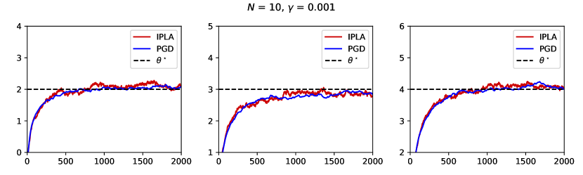
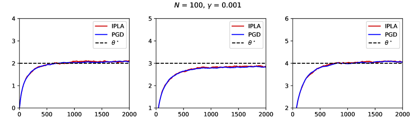
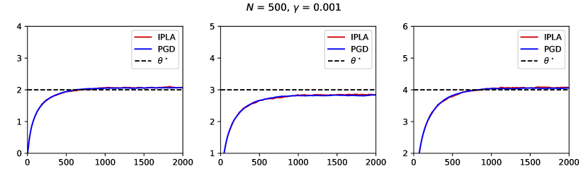
Figure 1: The performance of IPLA and PGD on the synthetic logistic regression problem. Each column corresponds to one of the components of the true parameter $\bar{\theta}^{\star}=[2,3,4]$. The top row corresponds to $N=10$, the middle row to $N=100$ and the bottom row to $N=500$. As expected, the PGD and IPLA perform similarly, especially as $N$ increases.

6.1 Bayesian logistic regression on synthetic data

We first compare the method proposed by Kuntz et al. (2023), which is termed particle gradient descent (PGD) and IPLA on a simple Bayesian regression task. We consider the Bayesian logistic regression LVM where for $\theta\in{}^{d_{\theta}}$

$$p_{\theta}(x) =\mathcal{N}(x;\theta,\sigma^{2}\textsf{Id}_{d_{x}}),\qquad\qquad p_{\theta}(y|x)=\prod_{j=1}^{d_{y}}s(v_{j}^{T}x)^{y_{j}}(1-s(v_{j}^{T}x))^{1-y_{j}},$$

with $d_{\theta}=d_{x}$, $s(u):=e^{u}/(1+e^{u})$ the logistic function and $\{v_{j}\}_{j=1}^{d_{y}}\in\mathbb{R}^{d_{x}}$ a set of covariates with corresponding binary responses $\{y_{j}\}_{j=1}^{d_{y}}\in\{0,1\}$. We assume that the value of $\sigma^{2}$ is fixed and known. In this section, we generate a set of synthetic $d_{x}$-dimensional covariates $v_{j}$ for $j=1,\dots,d_{y}$ and then generate our synthetic data $\{y_{j}\}_{j=1}^{d_{y}}$ sampling $y_{j}|\theta,x,v_{j}$ from a Bernoulli random variable with parameter $s(v_{j}^{T}x)$. The marginal likelihood is given by

$$k(\theta)=p_{\theta}(y)=(2\uppi\sigma^{2})^{-d_{x}/2}\int_{{}^{d_{x}}}\left(\prod_{j=1}^{d_{y}}s(v_{j}^{T}x)^{y_{j}}(1-s(v_{j}^{T}x))^{1-y_{j}}\right)\exp\left(-\|x-\theta\|^{2}/(2\sigma^{2})\right)\mathrm{d}x.$$

We then identify the performance of PGD and IPLA w.r.t. to the ground truth parameter. We note that only difference between PGD and IPLA is the noise in $\theta$-dimension, hence these algorithms perform similarly on a variety of tasks. In the next section, we will aim to identify a difference in their performance on the example provided on a real dataset.

6.1.1 Verifying A 1 and A 2

As shown in De Bortoli et al. (2021, Lemma S18), we have

$$U(\theta,x)=-\log p_{\theta}(x,y)=(d_{x}/2)\log(2\uppi\sigma^{2})-\sum_{j=1}^{d_{y}}\left(y_{j}\log(s(v_{j}^{T}x))+(1-y_{j})\log(s(-v_{j}^{T}x))\right)+\frac{\|x-\theta\|^{2}}{2\sigma^{2}},$$

and

$$\nabla_{\theta}U(\theta,x) =-\frac{x-\theta}{\sigma^{2}},\qquad\qquad\nabla_{x}U(\theta,x)=\frac{x-\theta}{\sigma^{2}}-\sum_{j=1}^{d_{y}}\left(y_{j}-s(v_{j}^{T}x)\right)v_{j}.$$

To check that A 1 holds observe that

$$\|\nabla U(v)-\nabla U(v^{\prime})\| \leq\|\nabla_{\theta}U(\theta,x)-\nabla_{\theta}U(\theta^{\prime},x^{\prime})\|+\|\nabla_{x}U(\theta,x)-\nabla_{x}U(\theta^{\prime},x^{\prime})\|$$

$$\leq\frac{2}{\sigma^{2}}(\|x-x^{\prime}\|+\|\theta-\theta^{\prime}\|)+\sum_{j=1}^{d_{y}}|s(v_{j}^{T}x)-s(v_{j}^{T}x^{\prime})|\|v_{j}\|$$

$$\leq\frac{2}{\sigma^{2}}(\|x-x^{\prime}\|+\|\theta-\theta^{\prime}\|)+\frac{1}{4}\|x-x^{\prime}\|\sum_{j=1}^{d_{y}}\|v_{j}\|^{2}$$

$$\leq(2\sigma^{-2}+1/4\sum_{j=1}^{d_{y}}\|v_{j}\|^{2})\left(\|\theta-\theta^{\prime}\|+\|x^{\prime}-x\|\right),$$

where we used the fact that the logistic function is Lipschitz continuous with Lipschitz constant $\sup_{u\in\real}|s^{\prime}(u)|=1/4$.

For A 2, consider the Hessian of $U$

$$\nabla^{2}U(v) =\frac{1}{\sigma^{2}}\begin{pmatrix}\textsf{Id}_{d_{\theta}}&-\textsf{Id}_{d_{x}}\\ -\textsf{Id}_{d_{x}}&\textsf{Id}_{d_{\theta}}\end{pmatrix}+\sum_{j=1}^{d_{y}}s(v_{j}^{T}x)(1-s(v_{j}^{T}x))v_{j}\otimes v_{j}.$$

The leftmost matrix has $2d_{\theta}$ strictly positive eigenvalues, and, as shown in Kuntz et al. (2023, Proposition 1, Appendix E.2) the rightmost matrix is positive definite, it follows that $\nabla^{2}U(v)$ is positive definite and thus $U$ is strongly convex.

6.1.2 Experimental Setup

We choose $d_{x}=d_{\theta}=3$ and $d_{y}=900$ and set $\bar{\theta}^{\star}=[2,3,4]$ to test the convergence of the parameter. We run the methods for $M=2000$ steps, with $N=10,100,500$ particles and $\gamma=0.001$. We set $\sigma=0.01$ and simulate $v_{j}\sim\textsf{Unif}(-1,1)^{\otimes d_{x}}$. We initialise the particles $X_{0}^{i,N}$ from a zero-mean Gaussian with covariance $\textsf{Id}_{d_{x}}$ and the initial parameter $\theta_{0}$ from a deterministic value $\theta_{0}=[0,0,0]$.

We see from Fig. 1 that both algorithms perform the same. This is expected since the only difference between the two algorithms is the noise in the $\theta$-dimension. As $N$ increases, the performance of both algorithms improves and IPLA gets closer to PGD, since the noise term in the $\theta$-component becomes smaller than the drift term. While PGD has limited theoretical guarantees, IPLA performs similarly to this method but has the additional advantage of having explicit theoretical guarantees on its convergence.

6.2 Bayesian logistic regression on Wisconsin cancer data

We next adopt a realistic example using the same setup in Kuntz and Lim (2023). In particular, in this section, we compare IPLA to PGD as well as more standard methods like mean-field variational inference (MFVI) and SOUL (De Bortoli et al., 2021).

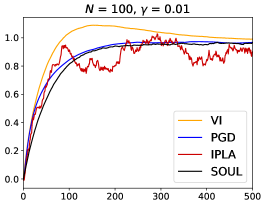
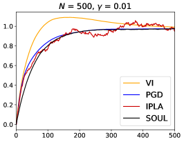
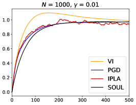
Figure 2: The performance of IPLA, PGD, MFVI and SOUL on the logistic regression experiment on real data. The left plot corresponds to $N=100$, the middle plot to $N=500$ and the right plot to $N=1000$. As expected, the PGD and IPLA perform similarly, especially as $N$ increases. We also note that SOUL is significantly slower compared to PGD and IPLA.

The setup in this section is a simplified version of the synthetic example in the last section, for which we verified our assumptions. Therefore, we do not verify our assumptions here again as they hold as a corollary of the proof in Sec. 6.1. We use in this section a breast cancer dataset with $d_{y}=683$ data points and $d_{x}=9$ latent variables (Wolberg et al., 1995). These $9$ latent variables correspond to latent “features” which are extracted from a digitised image of a fine needle aspirate (FNA) of a breast mass. The features describe characteristics of the cell nuclei present in the image (Wolberg et al., 1995). The data being $y=0$ or $y=1$ corresponds to whether the mass is benign or malignant. We use the setting provided by Kuntz and Lim (2023) and compare our method with PGD, MFVI and SOUL. For the implementation details of SOUL, PGD, and MFVI, we refer to Appendix E.2 of Kuntz et al. (2023).

For the estimation problem, we define

$$p_{\theta}(x) =\mathcal{N}(x;\theta\mathbf{1}_{d_{x}},5\textsf{Id}_{d_{x}}),$$

and our likelihood is

$$p(y|x) =\prod_{j=1}^{d_{y}}s(v_{j}^{T}x)^{y_{j}}(1-s(v_{j}^{T}x))^{1-y_{j}}.$$

In this example, we do not have a “ground truth” value as the data is real. We set $\gamma=0.01$ for all algorithms as this is the setup used in the fair comparison of algorithms in Kuntz et al. (2023). We run the algorithms for $M=500$ steps and vary the number of particles $N\in\{100,500,1000\}$. We note that, under this setting, SOUL gets increasingly expensive as it requires $N$ sequential ULA steps to update the parameter once, while PGD and IPLA can parallelise this computation. (Kuntz et al., 2023, Table 1) shows that for $N=100$ SOUL is at least 10 times slower than PGD on the same example considered here; since the computational cost of IPLA and PGD are identical we do not repeat the comparison.

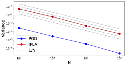
Figure 3: The convergence rate of the variance of the parameter estimates produced by PGD and IPLA over $100$ Monte Carlo runs for each $N\in\{10,100,1000,10000\}$. We can see that the $\mathcal{O}(1/N)$ convergence rate holds for the second moments as suggested by our results for IPLA. The PGD variance attains the same rate and it is lower. While this can be seen as an advantage for PGD in convex settings, we believe this is a feature of IPLA to escape local minima in the non-convex setting.

We present the results in Fig. 2, where we see that PGD and IPLA perform similarly. We also note that MFVI performs poorly compared to the other methods. This is expected as MFVI is a mean-field approximation and does not capture the correlation between the latent variables. We have also tested the variance of the estimates produced by PGD and IPLA over $100$ Monte Carlo runs for each $N\in\{10,100,1000,10000\}$ and present the results in Fig. 3. We see that the $\mathcal{O}(1/N)$ convergence rate holds for the second moments as suggested by our results for IPLA. The PGD variance attains the same rate but the overall variance of the estimates is significantly lower. While this can be seen as an advantage for PGD in convex settings, we believe this “sticky” behaviour is bad for non-convex optimisation. This noise is a feature of IPLA and can be beneficial to escape local minima in the non-convex setting.

7 Conclusions

In this paper we propose a new algorithm to perform maximum marginal likelihood estimation for latent variable models. The key observation of our work is that to obtain the maximum marginal likelihood estimator $\bar{\theta}^{\star}$, it is sufficient to sample from (1). Our algorithm combines ideas coming from the literature on optimisation using Langevin based approaches with an interacting particle system targetting (1) similar to that considered in Kuntz et al. (2023).

We exploit the connection with Langevin diffusions to provide convergence rates and nonasymptotic bounds which allow for careful tuning of the parameters needed to implement the algorithm (see Section 3.6). We obtain our main results (Theorem 1 and 2) under rather strong assumptions, however, our proof techniques can be applied under weaker assumptions and we expect that similar results will hold for nonconvex (dissipative) $U$ and can be obtained adapting the techniques of Zhang et al. (2023). Similarly, it is possible to relax the Lipschitz assumption on $U$ using the same framework.

While in many real world applications our strong convexity and Lipschitz continuity do not hold, we believe that our work constitutes the first building block towards developing and analysing these new class of algorithms and paves the way of a new class of results which can be proved using a similar machinery.

The experiments in Section 6 show that IPLA is competitive with other particle based methods (PGD; Kuntz et al. (2023)) and Langevin based methods (SOUL; De Bortoli et al. (2021)) and significantly outperforms variational inference approaches. The performances of IPLA and PGD are similar, as the latter is a modification of the former in which no noise is injected in the $\theta$-component. While this injection of noise might seem counterproductive, we found that it is crucial to obtain the explicit bounds in Theorem 1 and 2 and we believe it will be beneficial when dealing with non-convex problems as suggested by the wide literature on this class of optimisation problems. In addition, since for large values of $N$ the behaviour of IPLA and PGD gets closer, the theoretical results established in this work provide further validation and foundation for the work of Kuntz et al. (2023).

As observed in the introduction, any mechanism which samples from (1) can be used to perform maximum marginal likelihood estimation. Our IPLA algorithm is one example but we anticipate that other techniques from the sampling literature could be employed to achieve the same task. For example, Sharrock et al. (2023) propose two variations of PGD based on Stein-variational gradient flows (Liu and Wang, 2016) and coin sampling (Sharrock and Nemeth, 2023); we believe that similar ideas could be employed to provide equivalent variations of IPLA and we leave this for future work.

Appendix A Proofs of Section 3

Recall that we write continuous time processes such as (9) in bold, their Euler-Maruyama discretisation as non-bold characters, and the continuous interpolation (16) of the discretisation as barred characters (so that $\bar{\theta}_{n\gamma}=\theta_{n}$ and $\bar{\theta}_{t}$ is an approximation of $\bm{\theta}^{N}_{t}$). Finally, let us define, similarly to (7) the rescaled Euler-Maruyama discretisation

$$Z^{N}_{n}:=(\theta_{n},N^{-1/2}X^{1,N}_{n},...,N^{-1/2}X^{N,N}_{n}),$$ (24)

the rescaled interpolated discretisation

$$\bar{Z}^{N}_{t} :=(\bar{\theta}_{t},N^{-1/2}\bar{X}^{1,N}_{t},\ldots,N^{-1/2}\bar{X}^{N,N}_{t}),$$ (25)

and finally the rescaled continuous process

$$\bm{Z}^{N}_{t} :=(\bm{\theta}^{N}_{t},\bm{X}^{1,N}_{t},\ldots,\bm{X}^{N,N}_{t}).$$ (26)

We also denote the target measure of the rescaled system as $\pi_{\star,z}^{N}$. For notational convenience we define

$$\bm{V}^{i,N}_{t}=(\bm{\theta}^{N}_{t},\bm{X}^{i,N}_{t}),\;\;\;V^{i,N}_{n}=(\theta_{n},X^{i,N}_{n}),\;\;\;\bar{V}^{i,N}_{t}=(\bar{\theta}_{t},\bar{X}^{i,N}_{t}).$$ (27)

Note that

$$\frac{1}{N}\sum^{N}_{i=1}\|\bm{V}^{i,N}_{t}\|^{2}=\|\bm{Z}^{N}_{t}\|^{2},\;\;\;\frac{1}{N}\sum^{N}_{i=1}\|V^{i,N}_{n}\|^{2}=\|Z^{N}_{n}\|^{2},\;\;\;\frac{1}{N}\sum^{N}_{i=1}\|\bar{V}^{i,N}_{t}\|^{2}=\|\bar{Z}^{N}_{t}\|^{2},$$ (28)

a fact that we shall use often in the following proofs.

A.1 Proof of Proposition 4

Proof.

Let $v^{\star}=(\theta^{\star},x^{\star})$ be the minimiser of $U$, so $\nabla_{\theta}U(v^{\star})$ and $\nabla_{x}U(v^{\star})$ are vectors with identically zero entries. Let $z^{\star}=(\theta^{\star},\frac{1}{\sqrt{N}}x^{\star},...,\frac{1}{\sqrt{N}}x^{\star})$. We first bound ${\mathbb{E}}\left[\|\bm{Z}^{N}_{t}-z^{\star}\|^{2}\right]$ using Itô ’s formula

$${\mathbb{E}}\left[\|\bm{Z}^{N}_{t}-z^{\star}\|^{2}\right] ={\mathbb{E}}\left[\|Z^{N}_{0}-z^{\star}\|^{2}\right]-2{\mathbb{E}}\left[\int_{0}^{t}\left\langle\bm{\theta}^{N}_{s}-\theta^{\star},\frac{1}{N}\sum_{i=1}^{N}(\nabla_{\theta}U(\bm{V}^{i,N}_{s})-\nabla_{\theta}U(v^{\star}))\right\rangle\mathrm{d}s\right]$$

$$-2\frac{1}{N}\sum_{i=1}^{N}{\mathbb{E}}\left[\int_{0}^{t}\left\langle\bm{X}^{i,N}_{s}-x^{\star},(\nabla_{x}U(\bm{V}^{i,N}_{s})-\nabla_{x}U(v^{\star}))\right\rangle\mathrm{d}s\right]+2\frac{(Nd_{x}+d_{\theta})t}{N}$$

$$={\mathbb{E}}\left[\|Z^{N}_{0}-z^{\star}\|^{2}\right]-2\frac{1}{N}\sum_{i=1}^{N}\int_{0}^{t}{\mathbb{E}}\left[\left\langle\bm{V}^{i,N}_{s}-v^{\star},\nabla U(\bm{V}^{i,N}_{s})-\nabla U(v^{\star})\right\rangle\right]\mathrm{d}s$$

$$+2\frac{(Nd_{x}+d_{\theta})t}{N}.$$

We compute derivatives of both sides and apply the convexity assumption A 2 to obtain

$$\frac{{\mathrm{d}}{\mathbb{E}}\left[\|\bm{Z}^{N}_{t}-z^{\star}\|^{2}\right]}{{\mathrm{d}}t} =-2\frac{1}{N}\sum_{i=1}^{N}{\mathbb{E}}\left[\left\langle\bm{V}^{i,N}_{t}-v^{\star},\nabla U(\bm{V}^{i,N}_{t})-\nabla U(v^{\star})\right\rangle\right]+2\frac{Nd_{x}+d_{\theta}}{N}$$

$$\leq-2\mu{\mathbb{E}}\left[\|\bm{Z}^{N}_{t}-z^{\star}\|^{2}\right]+2\frac{Nd_{x}+d_{\theta}}{N}.$$

Consider next

$$\frac{{\mathrm{d}}e^{2\mu t}{\mathbb{E}}\left[\|\bm{Z}^{N}_{t}-z^{\star}\|^{2}\right]}{{\mathrm{d}}t} =2\mu e^{2\mu t}{\mathbb{E}}\left[\|\bm{Z}^{N}_{t}-z^{\star}\|^{2}\right]+e^{2\mu t}\frac{{\mathrm{d}}}{{\mathrm{d}}t}{\mathbb{E}}\left[\|\bm{Z}^{N}_{t}-z^{\star}\|^{2}\right]$$

$$\leq 2\mu e^{2\mu t}{\mathbb{E}}\left[\|\bm{Z}^{N}_{t}-z^{\star}\|^{2}\right]+e^{2\mu t}\left(-2\mu{\mathbb{E}}^{z_{0}}\left[\|\bm{Z}^{N}_{t}-z^{\star}\|^{2}\right]+2\frac{Nd_{x}+d_{\theta}}{N}\right)$$

$$=2e^{2\mu t}\frac{Nd_{x}+d_{\theta}}{N}.$$

Integrating both sides gives

$${\mathbb{E}}\left[\|\bm{Z}^{N}_{t}-z^{\star}\|^{2}\right]e^{2\mu t}-{\mathbb{E}}\left[\|Z_{0}^{N}-z^{\star}\|^{2}\right]\leq 2\frac{Nd_{x}+d_{\theta}}{N}\int_{0}^{t}e^{2\mu s}{\mathrm{d}}s.$$

This implies that

$${\mathbb{E}}\left[\|\bm{Z}^{N}_{t}-z^{\star}\|^{2}\right]\leq e^{-2\mu t}{\mathbb{E}}\left[\|Z_{0}^{N}-z^{\star}\|^{2}\right]+\frac{Nd_{x}+d_{\theta}}{N\mu}(1-e^{-2\mu t}).$$ (29)

Now we use the fact that $\pi_{\star}^{N}$ is the invariant measure of our SDE, i.e., $\pi_{\star}^{N}P_{t}^{N}=\pi_{\star}^{N}$ for the Markov kernel of our particle system $P_{t}^{N}$. It then follows by the definition (7) that the rescaled system has a rescaled invariant measure, that we denote $\pi^{N}_{\star,z}$, so that if we denote the rescaled transition kernel of $\bm{Z}^{N}_{t}$ as $\tilde{P}_{t}^{N}$ then one has $\pi^{N}_{\star,z}\tilde{P}_{t}^{N}=\pi^{N}_{\star,z}$. Hence by (29) one can write

$$\int_{{}^{d_{\theta}+Nd_{x}}}\|z-z^{\star}\|^{2}\pi^{N}_{\star,z}({\mathrm{d}}z) =\int_{{}^{d_{\theta}+Nd_{x}}}\int_{{}^{d_{\theta}+Nd_{x}}}\|z-z^{\star}\|^{2}\tilde{P}_{t}^{N}(z^{\prime},{\mathrm{d}}z)\pi^{N}_{\star,z}({\mathrm{d}}z^{\prime})$$

$$=\int_{{}^{d_{\theta}+Nd_{x}}}{\mathbb{E}}^{z^{\prime}}\left[\|\bm{Z}^{N}_{t}-z^{\star}\|^{2}\right]\pi^{N}_{\star,z}({\mathrm{d}}z^{\prime}),$$

$$\leq e^{-2\mu t}\int_{{}^{d_{\theta}+Nd_{x}}}\|z-z^{\star}\|^{2}\pi^{N}_{\star,z}({\mathrm{d}}z)+\frac{Nd_{x}+d_{\theta}}{N\mu}(1-e^{-2\mu t}),$$

which implies that

$$\int_{{}^{d_{\theta}+Nd_{x}}}\|z-z^{\star}\|^{2}\pi^{N}_{\star,z}(z){\mathrm{d}}z\leq\frac{d_{\theta}+Nd_{x}}{N\mu}.$$

We finalise this result by rewriting

$${\mathbb{E}}\left[\|\xi-z^{\star}\|^{2}\right]^{1/2}\leq\left(\frac{d_{\theta}+Nd_{x}}{N\mu}\right)^{1/2}$$ (30)

where $\xi$ be a $\mathcal{F}_{0}$-measurable (i.e. independent of the driving noise) random variable on $\mathbb{R}^{d_{\theta}+Nd_{x}}$ satisfying $\mathcal{L}(\xi)=\pi^{N}_{\star}$.

Now consider the IPS (9) with initial condition $\xi$, which we shall denote $(\tilde{\bm{\theta}}_{t},\tilde{\bm{X}}^{1,N}_{t},...,\tilde{\bm{X}}^{N,N}_{t})$. Then since by Proposition 2 one has that $\pi^{N}_{\star}$ is an invariant measure for (9), one may conclude that the law of the system is equal to $\pi^{N}_{*}$ for all time. Now consider the rescaling (15), and denote by $\pi^{N}_{z,*}$ the corresponding rescaled law of $\pi^{N}_{\star}$, so that in particular the rescaled initial condition $\xi_{z}:=(\xi_{\theta},N^{-1/2}\xi_{x_{1}},...,N^{-1/2}\xi_{x_{N}})$ satisfies $\mathcal{L}(\xi_{z})=\pi^{N}_{z,\star}$ and $\mathcal{L}(\tilde{\bm{Z}}^{N}_{t})=\pi^{N}_{z,\star}$ for all $t>0$ (where $\tilde{\bm{Z}}^{N}_{t}$ is given in the same way as (15)). Then one calculates

$${\mathbb{E}}\left[\|\bm{Z}^{N}_{t}-\tilde{\bm{Z}}_{t}^{N}\|^{2}\right] ={\mathbb{E}}[\|Z^{N}_{0}-\xi_{z}\|^{2}]-\frac{2}{N}\sum^{N}_{i=1}\mathbb{E}\left[\int^{t}_{0}\langle\nabla_{\theta}U(\bm{V}^{i,N}_{s})-\nabla_{\theta}U(\tilde{\bm{V}}^{i,N}_{s}),\bm{\theta}^{N}_{s}-\tilde{\bm{\theta}}_{s}\rangle\mathrm{d}s\right]$$

$$-\frac{2}{N}\sum^{N}_{i=1}\mathbb{E}\left[\int^{t}_{0}\langle\nabla_{x}U(\bm{V}^{i,N}_{s})-\nabla_{x}U(\tilde{\bm{V}}^{i,N}_{s}),\bm{X}^{i,N}_{s}-\tilde{\bm{X}}^{i,N}_{s}\rangle\mathrm{d}s\right]$$

$$={\mathbb{E}}[\|Z^{N}_{0}-\xi_{z}\|^{2}]-\frac{2}{N}\sum^{N}_{i=1}\mathbb{E}\left[\int^{t}_{0}\langle\nabla U(\bm{V}^{i,N}_{s})-\nabla U(\tilde{\bm{V}}^{i,N}_{s}),\bm{V}^{i,N}_{s}-\tilde{\bm{V}}^{i,N}_{s}\rangle\mathrm{d}s\right].$$

Then we can differentiate, apply the convexity assumption A 2 to each term in the sum and then the identity (28) to obtain

$$\frac{\mathrm{d}}{\mathrm{d}t}{\mathbb{E}}\left[\|\bm{Z}^{N}_{t}-\tilde{\bm{Z}}_{t}^{N}\|^{2}\right]\leq-2\mu\mathbb{E}\left[\|\bm{Z}^{N}_{s}-\tilde{\bm{Z}}_{s}\|^{2}\right],$$

so that

$$\frac{\mathrm{d}}{\mathrm{d}t}\biggr{(}e^{2\mu t}{\mathbb{E}}\left[\|\bm{Z}^{N}_{t}-\tilde{\bm{Z}}_{t}^{N}\|^{2}\right]\biggr{)}\leq 0,$$

and therefore by the Fundamental Theorem of Calculus, since ${\mathbb{E}}[\|\bm{Z}^{N}_{0}-\tilde{\bm{Z}}_{0}^{N}\|^{2}]={\mathbb{E}}[\|Z^{N}_{0}-\xi_{z}\|^{2}]$, integrating the above on $[0,t]$ and dividing by $e^{2\mu t}$ yields

$${\mathbb{E}}\left[\|\bm{Z}^{N}_{t}-\tilde{\bm{Z}}_{t}^{N}\|^{2}\right]\leq e^{-2\mu t}{\mathbb{E}}[\|Z^{N}_{0}-\xi_{z}\|^{2}].$$

Now note that by the definition of the Wassserstein distance, and since $\mathcal{L}(\tilde{\bm{\theta}}_{t})=\pi^{N}_{\Theta}$, one may write

$$W_{2}(\mathcal{L}(\bm{\theta}^{N}_{t}),\pi^{N}_{\Theta})^{2}\leq{\mathbb{E}}[\|\bm{\theta}^{N}_{t}-\tilde{\bm{\theta}}_{t}\|^{2}]\leq{\mathbb{E}}[\|\bm{Z}^{N}_{t}-\tilde{\bm{Z}}^{N}_{t}\|^{2}]\leq e^{-2\mu t}{\mathbb{E}}[\|Z^{N}_{0}-\xi_{z}\|^{2}],$$

which implies

$$W_{2}(\mathcal{L}(\bm{\theta}^{N}_{t}),\pi^{N}_{\Theta})\leq e^{-\mu t}{\mathbb{E}}[\|Z^{N}_{0}-\xi_{z}\|^{2}]^{1/2}.$$ (31)

Our strategy now is to bound ${\mathbb{E}}[\|Z^{N}_{0}-\xi_{z}\|^{2}]^{1/2}$ using a triangle inequality. Note that ${\mathbb{E}}[\|Z^{N}_{0}-\xi_{z}\|^{2}]^{1/2}$ is a norm, hence we can write

$${\mathbb{E}}[\|Z^{N}_{0}-\xi_{z}\|^{2}]^{1/2} \leq{\mathbb{E}}[\|Z^{N}_{0}-z^{\star}\|^{2}]^{1/2}+{\mathbb{E}}[\|z^{\star}-\xi_{z}\|^{2}]^{1/2}.$$

Using (30) for the last term concludes the result. ∎

A.2 Euler–Maruyama discretisation

Remark 2.

In the following we let $C>0$ be a generic constant that changes from line to line, independent of $d_{\theta},d_{x}$ and the stepsize $\gamma>0$.

A.2.1 Moment and increment bounds

Lemma 1.

Let A 1, A 2, A 3 hold . Then for every $\gamma_{0}\in(0,\min\{L^{-1},2\mu^{-1}\})$ there exists a constant $C>0$ independent of $t,n,N,\gamma,d_{\theta},d_{x}$ such that for every $\gamma\in(0,\gamma_{0})$, $n\in\mathbb{N}$,

$${\mathbb{E}}[\lvert\lvert Z^{N}_{n}\rvert\rvert^{2}]\leq C(1+d_{\theta}/N+d_{x}).$$

Proof.

Let $v^{\star}=(\theta^{\star},x^{\star})$ be the minimiser of the function $U$ (where $\overline{\theta}^{\star}\not=\theta^{\star}$ in general), and $z^{\star}=(\theta^{\star},N^{-1/2}x^{\star},....,N^{-1/2}x^{\star})\in\mathbb{R}^{d_{\theta}+Nd_{x}}$. Recall that a standard Gaussian on $\mathbb{R}^{d}$ has second moment equal to $d$, so that using the definition (27) of the process $V^{i,N}_{t}$ one has

$$\mathbb{E}\left[\|Z^{N}_{n+1}-z^{\star}\|^{2}\right] \leq\mathbb{E}\left[\|Z^{N}_{n}-z^{\star}\|^{2}\right]+\gamma^{2}\mathbb{E}\left[\biggr{(}\frac{1}{N}\sum_{i=1}^{N}\|\nabla_{\theta}U(V^{i,N}_{n})\|\biggr{)}^{2}\right]+\frac{2\gamma d_{\theta}}{N}$$

$$-\frac{2\gamma}{N}\sum_{j=1}^{N}{\mathbb{E}}\left[\langle\theta_{n}-\theta^{\star},\nabla_{\theta}U(V_{n}^{j,N})\rangle\right]$$

$$+\frac{1}{N}\sum_{i=1}^{N}\biggr{(}\gamma^{2}\mathbb{E}\left[\|\nabla_{x}U(V_{n}^{i,N})\|^{2}\right]+2\gamma d_{x}-2\gamma\mathbb{E}\left[\langle X_{n}^{i,N}-x^{\star},\nabla_{x}U(V_{n}^{i,N})\rangle\right]\biggr{)}.$$

Now note that

$$\frac{1}{N}\biggr{(}\sum_{i=1}^{N}\langle\theta,\nabla_{\theta}U(\theta,x_{i})\rangle+\langle x_{i},\nabla_{x}U(\theta,x_{i})\rangle\biggr{)}=\frac{1}{N}\sum_{i=1}^{N}\langle(\theta,x_{i}),\nabla U(\theta,x_{i})\rangle,$$

and furthermore, by Young’s inequality one has

$$\biggr{(}\frac{1}{N}\sum_{i=1}^{N}a_{i}\biggr{)}^{2}\leq\frac{1}{N}\sum_{i=1}^{N}a_{i}^{2},$$ (32)

which one may apply as well as the fact that

$$\|\nabla U\|^{2}=\|\nabla U_{\theta}\|^{2}+\|\nabla U_{x}\|^{2}$$ (33)

and $\nabla U(v^{\star})=0$ to obtain that

$$\mathbb{E}\left[\|Z^{N}_{n+1}-z^{\star}\|^{2}\right] \leq\mathbb{E}\left[\|Z^{N}_{n}-z^{\star}\|^{2}\right]-\frac{2\gamma}{N}\mathbb{E}\left[\sum_{i=1}^{N}\langle V^{i,N}_{N}-v^{\star},\nabla U(V^{i,N}_{n})-\nabla U(v^{\star})\rangle\right]$$

$$+2\gamma(\frac{d_{\theta}}{N}+d_{x})+\frac{\gamma^{2}}{N}\mathbb{E}\left[\biggr{(}\sum_{i=1}^{N}\|\nabla U(V^{i,N}_{n})-\nabla U(v^{\star})\|^{2}\biggr{)}\right].$$ (34)

Furthermore, since $U$ is convex, we may use co-coercivity (see Theorem 1 in Gao and Pavel (2018)), given as

$$\langle\nabla U(x)-\nabla U(y),x-y\rangle\geq\frac{1}{L}\|\nabla U(x)-\nabla U(y)\|^{2},$$

for every $x,y\in\mathbb{R}^{d}$, to conclude for every $\gamma<\frac{1}{L}$

$$-\frac{\gamma}{N}\mathbb{E}\left[\sum_{i=1}^{N}\langle V^{i,N}_{N}-v^{\star},\nabla U(V^{i,N}_{n})-\nabla U(v^{\star})\rangle\right]+\frac{\gamma^{2}}{N}\mathbb{E}\left[\biggr{(}\sum_{i=1}^{N}\|\nabla U(V^{i,N}_{n})-\nabla U(v^{\star})\|^{2}\biggr{)}\right]\leq 0.$$

Therefore by the convexity assumption A 2 and (28)

$$\mathbb{E}\left[\|Z^{N}_{n+1}-z^{\star}\|^{2}\right] \leq\mathbb{E}\left[\|Z^{N}_{n}-z^{\star}\|^{2}\right]-\frac{\gamma}{N}\mathbb{E}\left[\sum_{i=1}^{N}\langle V^{i,N}_{N}-v^{\star},\nabla U(V^{i,N}_{n})-\nabla U(v^{\star})\rangle\right]+2\gamma(\frac{d_{\theta}}{N}+d_{x})$$

$$\leq(1-\mu\gamma)\mathbb{E}\left[\|Z^{N}_{n}-z^{\star}\|^{2}\right]+2\gamma(\frac{d_{\theta}}{N}+d_{x}).$$

Now recall that for $\alpha\in(-1,1)$, $\beta>0$ and a sequence $x_{n}\in\mathbb{R}$ satisfying $x_{n+1}\leq\alpha x_{n}+\beta$ one has

$$x_{n}\leq\alpha^{n}x_{0}+\beta\sum^{n}_{i=1}\alpha^{i-1}\leq x_{0}+\frac{\beta}{1-\alpha}.$$ (35)

Using this bound, for every $\gamma<\frac{2}{\mu}$ one obtains that

$$\mathbb{E}\left[\|Z^{N}_{n+1}-z^{\star}\|^{2}\right]\leq{\mathbb{E}}[\|Z^{N}_{0}-z^{\star}\|^{2}]+\mu^{-1}(\frac{d_{\theta}}{N}+d_{x}),$$

and as a result, by A 3 one has

$$\mathbb{E}\left[\|Z^{N}_{n}\|^{2}\right] \leq 2\mathbb{E}\left[\|Z_{n}^{N}-z^{\star}\|^{2}\right]+2\|z^{\star}\|^{2}$$

$$\leq C(1+\frac{d_{\theta}}{N}+d_{x}),$$

where $C>0$ is the generic constant introduced in Remark 2. ∎

Lemma 2.

Let A 1, A 2, A 3 hold and consider the interpolated discretisation (25). Then for every $\gamma_{0}\in(0,\min\{L^{-1},2\mu^{-1}\})$ there exists a constant $C>0$ independent of $t,n,N,\gamma,d_{\theta},d_{x}$ such that for every $\gamma\in(0,\gamma_{0})$, $n\in\mathbb{N}$, $t\geq 0$

$${\mathbb{E}}[\lvert\lvert\bar{Z}^{N}_{t}-\bar{Z}^{N}_{\kappa_{\gamma}(t)}\rvert\rvert^{2}]\leq C(1+d_{\theta}/N+d_{x})\gamma.$$

and

$${\mathbb{E}}[\lvert\lvert\bm{Z}^{N}_{t}-\bm{Z}^{N}_{\kappa_{\gamma}(t)}\rvert\rvert^{2}]\leq C(1+d_{\theta}/N+d_{x})\gamma.$$ (36)

Proof.

Recall that $\kappa_{\gamma}(t)=\gamma\lfloor\gamma^{-1}t\rfloor$ is the projection back onto the grid $\{0,\gamma,2\gamma,..\}$. Using the interpolation $\bar{Z}^{N}_{t}$ of $Z^{N}_{n}$ given in (24), given that $\bar{Z}^{N}_{\kappa_{\gamma}(t)}=Z^{N}_{\kappa_{\gamma}(t)/\gamma}$ one calculates by (28) and (33), and since the second moment of a standard $d$-dimensional Gaussian is $d$, that

$$\mathbb{E}\left[\|\bar{Z}^{N}_{t}-\bar{Z}^{N}_{\kappa_{\gamma}(t)}\|^{2}\right]\leq 2\lvert t-\kappa_{\gamma}(t)\rvert(\frac{d_{\theta}}{N}+d_{x})+\frac{\lvert t-\kappa_{\gamma}(t)\rvert^{2}}{N}\mathbb{E}\left[\sum_{i=1}^{N}\|\nabla U(V^{i,N}_{\kappa_{\gamma}(t)/\gamma})\|^{2}\right],$$

so that applying the Lipschitz assumption A 1 and (28) one has, since $\lvert t-\kappa_{\gamma}(t)\rvert\leq 1$,

$$\mathbb{E}\left[\|\bar{Z}^{N}_{t}-\bar{Z}^{N}_{\kappa_{\gamma}(t)}\|^{2}\right] \leq C\lvert t-\kappa_{\gamma}(t)\rvert(d_{\theta}/N+d_{x}+\frac{1}{N}\sum_{i=1}^{N}{\mathbb{E}}[\|V^{i,N}_{\kappa_{\gamma}(t)/\gamma}\|^{2}])\leq C\gamma(1+\|Z^{N}_{\kappa_{\gamma}(t)/\gamma}\|^{2}),$$

and therefore that the first stated result follows from Lemma 1. We shall use a similar argument to prove (36). In particular, we have by (29) and A 3 that

$${\mathbb{E}}[\|\bm{Z}^{N}_{t}\|^{2}]\leq C(1+d_{\theta}/N+d_{x}),$$

so by Itô ’s formula

$${\mathbb{E}}[\|\bm{Z}^{N}_{t}-\bm{Z}^{N}_{\kappa_{\gamma}(t)}\|^{2}] =-{\mathbb{E}}\biggr{[}\int^{t}_{\kappa_{\gamma}(t)}\biggr{(}\frac{2}{N}\sum_{i=1}^{N}\langle\nabla_{\theta}U(\bm{V}^{i,N}_{u}),\bm{V}^{i,N}_{u}\rangle+\frac{2}{N}\sum_{i=1}^{N}\langle\nabla_{x}U(\bm{V}^{i,N}_{u}),\bm{V}^{i,N}_{u}\rangle+2(d_{\theta}/N+d_{x})\biggr{)}\mathrm{d}u\biggr{]}$$

$$=\int^{t}_{\kappa_{\gamma}(t)}\biggr{(}\frac{2}{N}\sum_{i=1}^{N}{\mathbb{E}}[\langle\nabla U(\bm{V}^{i,N}_{u}),\bm{V}^{i,N}_{u}\rangle]+2(d_{\theta}/N+d_{x})\biggr{)}\mathrm{d}u,$$

and therefore by Cauchy-Schwarz, Young’s inequality, the Lipschitz Assumption A 1 and (28) one has

$${\mathbb{E}}[\|\bm{Z}^{N}_{t}-\bm{Z}^{N}_{\kappa_{\gamma}(t)}\|^{2}] \leq C\int^{t}_{\kappa_{\gamma}(t)}\biggr{(}\frac{1}{N}\sum_{i=1}^{N}(1+\|\bm{V}^{i,N}_{u}\|^{2})+d_{\theta}/N+d_{x}\biggr{)}\mathrm{d}u$$

$$\leq C\int^{t}_{\kappa_{\gamma}(t)}\biggr{(}1+{\mathbb{E}}[\|\bm{Z}^{N}_{u}\|^{2}]+d_{\theta}/N+d_{x}\biggr{)}\mathrm{d}u$$

$$\leq C(1+d_{\theta}/N+d_{x})\lvert t-\kappa_{\gamma}(t)\rvert,$$

where $C>0$ is the generic constant introduced in Remark 2. ∎

A.2.2 Proof of Proposition 5

Proof.

In order to prove (18) we consider the convergence of the entire rescaled discretised IPS $Z^{N}_{n}$ to the original continuous rescaled process $\bm{Z}^{N}_{t}$. In particular, noting that $Z^{N}_{n}$ is an approximation of $\bm{Z}^{N}_{n\gamma}$, we shall prove that

$$\mathbb{E}\left[\|Z^{N}_{n}-\bm{Z}^{N}_{n\gamma}\|^{2}\right]\leq C(1+d_{\theta}/N+d_{x})\gamma,$$ (37)

at which point (18) follows immediately. The interpolated process $\bar{Z}^{N}_{t}$ given as

$$\bar{Z}^{N}_{t}:=(\bar{\theta}_{t},N^{-1/2}\bar{X}^{i,N}_{t},...,N^{-1/2}\bar{X}^{i,N}_{t}).$$

via the interpolated discretisation (16) satisfies $\bar{Z}^{N}_{\gamma n}=Z^{N}_{n}$, so we shall actually prove

$$\mathbb{E}\left[\|\bar{Z}^{N}_{t}-\bm{Z}^{N}_{t}\|^{2}\right]\leq C(1+d_{\theta}/N+d_{x})\gamma.$$ (38)

Since $\bar{Z}^{N}_{t}$ is an Itô process, so we can apply Itô’s formula for $x\mapsto\lvert x\rvert^{2}$ to obtain

$$\lvert\lvert\bar{Z}^{N}_{t}-\bm{Z}^{N}_{t}\rvert\rvert^{2} =-\frac{1}{N}\sum_{i=1}^{N}\int^{t}_{0}\langle\nabla_{\theta}U(\bar{\theta}_{\kappa_{\gamma}(s)},\bar{X}_{\kappa_{\gamma}(s)}^{i,N})-\nabla_{\theta}U(\bm{\theta}^{N}_{s},\bm{X}^{i,N}_{s}),\bar{\theta}_{s}-\bm{\theta}^{N}_{s}\rangle\mathrm{d}s$$

$$-\frac{1}{N}\sum_{i=1}^{N}\int^{t}_{0}\langle\nabla_{x}U(\bar{\theta}_{\kappa_{\gamma}(s)},\bar{X}_{\kappa_{\gamma}(s)}^{i,N})-\nabla_{x}U(\bm{\theta}^{N}_{s},\bm{X}^{i,N}_{s}),\bar{X}^{i,N}_{s}-\bm{X}^{i,N}_{s}\rangle\mathrm{d}s$$

$$=-\frac{1}{N}\sum_{i=1}^{N}\int^{t}_{0}\langle\nabla U(\bar{V}^{i,N}_{\kappa_{\gamma}(s)})-\nabla U(\bm{V}_{s}),\bar{V}^{i,N}_{s}-\bm{V}^{i,N}_{s}\rangle\mathrm{d}s,$$

where $\bar{V}^{i,N}_{t}=(\bar{\theta}_{t},\bar{X}^{i,N}_{t})$ and $\bm{V}^{i,N}_{t}=(\bm{\theta}^{N}_{t},\bm{X}^{i,N}_{t})$ for $i=1,2,...,N$ and $t>0$. For convenience let us define

$$e^{i,N}_{t}:=\bar{V}^{i,N}_{t}-\bm{V}^{i,N}_{t},\;\;e_{t}=\bar{Z}^{N}_{t}-\bm{Z}^{N}_{t},$$

so that in particular

$$\frac{1}{N}\sum^{N}_{i=1}\|e^{i,N}_{t}\|^{2}=\|e_{t}\|^{2}.$$ (39)

Using the above, one may apply Itô’s formula again for $x\mapsto e^{\mu t/2}\lvert x\rvert^{2}$ to obtain

$$e^{\mu t/2}\|e_{t}\|^{2}=\int^{t}_{0}\frac{\mu}{2}e^{\mu s/2}\|e_{s}\|^{2}+\int^{t}_{0}e^{\mu s/2}\biggr{(}-\frac{1}{N}\sum_{i=1}^{N}\langle\nabla U(\bar{V}^{i,N}_{\kappa_{\gamma}(s)})-\nabla U(\bm{V}_{s}),e^{i,N}_{s}\rangle\biggr{)}\mathrm{d}s.$$ (40)

Let us now bound $-N^{-1}\sum_{i=1}^{N}\langle\nabla U(\bar{V}^{i,N}_{\kappa_{\gamma}(s)})-\nabla U(\bm{V}_{s}),e^{i,N}_{s}\rangle$ by splitting as

$$-\frac{1}{N}\sum_{i=1}^{N}\langle\nabla U(\bar{V}^{i,N}_{\kappa_{\gamma}(s)})-\nabla U(\bm{V}_{s}),e^{i,N}_{s}\rangle =-\frac{1}{N}\sum_{i=1}^{N}\langle\nabla U(\bar{V}^{i,N}_{s})-\nabla U(\bm{V}_{s}^{i,N}),e^{i,N}_{s}\rangle$$

$$-\frac{1}{N}\sum_{i=1}^{N}\langle\nabla U(\bar{V}^{i,N}_{\kappa_{\gamma}(s)})-\nabla U(\bar{V}^{i,N}_{s}),e^{i,N}_{s}\rangle$$

$$:=r_{1}(s)+r_{2}(s)$$ (41)

We then control the first term in the same way as in the proof of Proposition 3, and the discretisation error $r_{2}(s)$ using standard bounds for stochastic processes. Specifically, for the former we have by the convexity assumption A 2 and a variation on (28) that

$$r_{1}(s) =-\frac{1}{N}\sum_{i=1}^{N}\langle\nabla U(\bar{V}^{i,N}_{s})-\nabla U(\bm{V}_{s}),e^{i,N}_{s}\rangle$$

$$\leq-\mu\frac{1}{N}\sum_{i=1}^{N}\|V_{s}^{i,N}-\bm{V}^{i,N}_{s}\|^{2}$$

$$\leq-\mu\|e_{s}\|^{2}.$$ (42)

For the second part, the Cauchy-Schwarz inequality, Young’s inequality and A 1 give

$$r_{2}(s) =\frac{1}{N}\sum_{i=1}^{N}\langle\nabla U(\bar{V}^{i,N}_{s})-\nabla U(\bar{V}^{i,N}_{\kappa_{\gamma}(s)}),e^{i,N}_{s}\rangle$$

$$\leq\frac{1}{N}\sum_{i=1}^{N}\|\nabla U(\bar{V}^{i,N}_{s})-\nabla U(\bar{V}^{i,N}_{\kappa_{\gamma}(s)})\|\cdot\|e^{i,N}_{s}\|$$

$$\leq\frac{1}{N}\sum_{i=1}^{N}(\frac{1}{2\mu}\|\nabla U(\bar{V}^{i,N}_{\kappa_{\gamma}(s)})-\nabla U(\bar{V}^{i,N}_{s})\rvert\rvert^{2}+\frac{\mu}{2}\|e^{i,N}_{s}\|^{2})$$

$$\leq C\|\bar{Z}^{N}_{\kappa_{\gamma}(s)}-\bar{Z}^{N}_{s}\|^{2}+\frac{\mu}{2}\|e_{s}\|^{2}.$$ (43)

Therefore, by Lemma 2, combining (A.2.2) and (A.2.2) into (A.2.2) and taking expectation one obtains

$$-\frac{1}{N}\sum_{i=1}^{N}{\mathbb{E}}[\langle\nabla U(\bar{V}^{i,N}_{\kappa_{\gamma}(s)})-\nabla U(\bm{V}_{s}),e^{i,N}_{s}\rangle]\leq C(1+d_{\theta}/N+d_{x})\gamma-\frac{\mu}{2}{\mathbb{E}}[\|e_{s}\|^{2}],$$ (44)

which one substitutes into (40) to obtain

$$e^{\mu t/2}{\mathbb{E}}[\|e_{t}\|^{2}]\leq\int^{t}_{0}C\gamma e^{\mu s/2}\mathrm{d}s\leq C(1+d_{\theta}/N+d_{x})\gamma e^{\mu t/2},$$ (45)

at which point the result follows by dividing through by $e^{\mu t/2}$. ∎

A.2.3 Proof of Proposition 6

Proof.

We follow a similar strategy to the proof of Proposition 5, but using a slightly more delicate strategy to bound $r_{2}$, defined in (A.2.2). In particular, note that if we denote

$$\zeta^{i,N}_{s}:=\sqrt{2}(N^{-1/2}(\bm{B}^{0,N}_{s}-\bm{B}^{0,N}_{\kappa_{\gamma}(s)}),\bm{B}^{i,N}_{s}-\bm{B}^{i,N}_{\kappa_{\gamma}(s)})$$

then

$$\bar{V}^{i,N}_{s}=\bar{V}^{i,N}_{\kappa_{\gamma}(s)}-(s-\kappa_{\gamma}(s))\biggr{(}\frac{1}{N}\sum^{N}_{j=1}\nabla_{\theta}U(\bar{V}^{j,N}_{\kappa_{\gamma}(s)}),\;\nabla_{x}U(\bar{V}^{j,N}_{\kappa_{\gamma}(s)})\biggr{)}+\zeta^{i,N}_{s},$$

so we can split $r_{2}$ as

$$r_{2}(s) =\frac{1}{N}\sum_{i=1}^{N}\langle\nabla U(\bar{V}^{i,N}_{s})-\nabla U(\bar{V}^{i,N}_{\kappa_{\gamma}(s)}),e^{i,N}_{s}\rangle$$

$$=\frac{1}{N}\sum_{i=1}^{N}\langle\nabla U(\bar{V}^{i,N}_{s})-\nabla U(\bar{V}^{i,N}_{\kappa_{\gamma}(s)}+\zeta^{i,N}_{s}),e^{i,N}_{s}\rangle$$

$$+\frac{1}{N}\sum_{i=1}^{N}\langle\nabla U(\bar{V}^{i,N}_{\kappa_{\gamma}(s)}+\zeta^{i,N}_{s})-\nabla U(\bar{V}^{i,N}_{\kappa_{\gamma}(s)}),e^{i,N}_{s}\rangle$$

$$:=r_{2,1}(s)+r_{2,2}(s).$$

Firstly let us bound $r_{2,1}$. By Cauchy-Schwarz, Young’s inequality and (39) one has

$$r_{2,1}(s) \leq\frac{1}{N}\sum_{i=1}^{N}(C\|\bar{V}^{i,N}_{s}-\bar{V}^{i,N}_{\kappa_{\gamma}(s)}-\zeta^{i,N}_{s}\|^{2}+\frac{\mu}{6}\|e^{i,N}_{s}\|^{2})$$

$$\leq\gamma^{2}\frac{1}{N}\sum_{i=1}^{N}C\biggr{(}\biggr{\|}\frac{1}{N}\sum_{j=1}^{N}\nabla_{\theta}U(\bar{V}^{j,N}_{\kappa_{\gamma}(s)})\biggr{\|}^{2}+\|\nabla_{x}U(\bar{V}^{i,N}_{\kappa_{\gamma}(s)})\|^{2}\biggr{)}+\frac{\mu}{6}\|e_{t}\|^{2}.$$

Now one may apply (32) to terms arising from the sum in the first term above, so that by the Lipschitz assumption and Lemma 2

$${\mathbb{E}}[r_{2,1}(s)] \leq\gamma^{2}\frac{C}{N}\sum_{i=1}^{N}{\mathbb{E}}[\|\nabla U(\bar{V}^{i,N}_{\kappa_{\gamma}(s)})\|^{2}]+\frac{\mu}{6}{\mathbb{E}}[\|e_{s}\|^{2}]$$

$$\leq C(1+d_{\theta}/N+d_{x})\gamma^{2}+\frac{\mu}{6}{\mathbb{E}}[\|e_{s}\|^{2}]$$ (46)

Now we shall need to split $r_{2,2}$ as follows

$$r_{2,2}(s) =\frac{1}{N}\sum_{i=1}^{N}\langle\nabla U(\bar{V}^{i,N}_{\kappa_{\gamma}(s)}+\zeta^{i,N}_{s})-\nabla U(\bar{V}^{i,N}_{\kappa_{\gamma}(s)}),e^{i,N}_{s}\rangle$$

$$=\frac{1}{N}\sum_{i=1}^{N}\langle\nabla U(\bar{V}^{i,N}_{\kappa_{\gamma}(s)}+\zeta^{i,N}_{s})-\nabla U(\bar{V}^{i,N}_{\kappa_{\gamma}(s)})-\Delta U(\bar{V}^{i,N}_{\kappa_{\gamma}(s)})\zeta^{i,N}_{s},e^{i,N}_{s}\rangle$$

$$+\frac{1}{N}\sum_{i=1}^{N}\langle\Delta U(\bar{V}^{i,N}_{\kappa_{\gamma}(s)})\zeta^{i,N}_{s},e^{i,N}_{s}-e^{i,N}_{\kappa_{\gamma}(s)}\rangle$$

$$+\frac{1}{N}\sum_{i=1}^{N}\langle\Delta U(\bar{V}^{i,N}_{\kappa_{\gamma}(s)})\zeta^{i,N}_{s},e^{i,N}_{\kappa_{\gamma}(s)}\rangle$$

$$:=r_{2,2,1}(s)+r_{2,2,2}(s)+r_{2,2,3}(s).$$

For the first term in this splitting we use the smoothness assumption A 4 and Kumar and Sabanis (2019, Lemma 5) with $\gamma=0$ to obtain by the definition of $\zeta^{i,N}_{t}$ (since a standard Gaussian on $\mathbb{R}^{d}$ has fourth moment equal to $Cd^{2}$) that

$${\mathbb{E}}[r_{2,2,1}(s)] \leq\frac{1}{N}\sum_{i=1}^{N}(C{\mathbb{E}}[\|\nabla U(\bar{V}^{i,N}_{\kappa_{\gamma}(t)}+\zeta^{i,N}_{s})-\nabla U(\bar{V}^{i,N}_{\kappa_{\gamma}(s)})-\Delta U(\bar{V}^{i,N}_{\kappa_{\gamma}(s)})\zeta^{i,N}_{s}\|^{2}]+\frac{\mu}{6}{\mathbb{E}}[\|e^{i,N}_{s}\|^{2}])$$

$$\leq C\frac{1}{N}\sum_{i=1}^{N}{\mathbb{E}}[\|\zeta^{i,N}_{s}\|^{4}]+\frac{\mu}{6}{\mathbb{E}}[\|e_{t}\|^{2}]$$

Now note that by definition, since a standard Gaussian $\zeta$ on $\mathbb{R}^{d}$ satisfies ${\mathbb{E}}[\|\zeta\|^{2}]=d$, ${\mathbb{E}}[\|\zeta\|^{4}]=Cd^{2}$, one has

$${\mathbb{E}}[\|\zeta^{i,N}_{s}\|^{4}]=C(N^{-2}d_{\theta}^{2}+d_{x}^{2}+N^{-1}d_{\theta}d_{x})\gamma^{2}\leq C(d_{\theta}/N+d_{x})^{2}\gamma^{2},$$

so that

$${\mathbb{E}}[r_{2,2,1}(s)]\leq C(N^{-1}d_{\theta}+d_{x})^{2}\gamma^{2}+\frac{\mu}{6}{\mathbb{E}}[\|e_{s}\|^{2}].$$ (47)

To control $r_{2,2,2}$, first by Young’s inequality (recalling that the expresion in brackets below is an element of $\mathbb{R}^{d_{\theta}+d_{x}}$ and not an inner product) we have the bound

$$\|\Delta U(\bar{V}^{i,N}_{\kappa_{\gamma}(s)})\zeta^{i,N}_{t}\|\cdot\|e^{i,N}_{s}-e^{i,N}_{\kappa_{\gamma}(s)}\|$$

$$\leq\|\Delta U(\bar{V}^{i,N}_{\kappa_{\gamma}(t)})\zeta^{i,N}_{s}\|\cdot\int^{s}_{\kappa_{\gamma}(s)}\biggr{\|}\biggr{(}\frac{1}{N}\sum_{j=1}^{N}(\nabla_{\theta}U(\bm{V}_{u}^{j,N})-\nabla_{\theta}U(\bar{V}_{\kappa_{\gamma}(s)}^{j,N})),\nabla_{x}U(\bm{V}_{u}^{i,N})-\nabla_{x}U(\bar{V}_{\kappa_{\gamma}(s)}^{i,N})\biggr{)}\biggr{\|}\mathrm{d}u$$

$$\leq\int^{s}_{\kappa_{\gamma}(s)}\biggr{(}C\|\Delta U(\bar{V}^{i,N}_{\kappa_{\gamma}(s)})\zeta^{i,N}_{s}\|^{2}+\frac{\mu}{18L}\biggr{\|}\frac{1}{N}\sum_{j=1}^{N}(\nabla_{\theta}U(\bm{V}_{u}^{j,N})-\nabla_{\theta}U(\bar{V}_{\kappa_{\gamma}(s)}^{j,N}))\biggr{\|}^{2}\biggr{)}\mathrm{d}u$$

$$+\int^{s}_{\kappa_{\gamma}(s)}\frac{\mu}{18L}\|\nabla_{x}U(\bm{V}_{u}^{i,N})-\nabla_{x}U(\bar{V}_{\kappa_{\gamma}(s)}^{i,N})\|^{2}\mathrm{d}u.$$

Now note that by the independence of $\zeta^{i,N}_{t}$ from $\bar{V}^{i,N}_{\kappa_{\gamma}(t)}$ and A 4 one has

$${\mathbb{E}}[\|\Delta U(\bar{V}^{i,N}_{\kappa_{\gamma}(s)})\zeta^{i,N}_{s}\|^{2}] \leq{\mathbb{E}}[\|\Delta U(\bar{V}^{i,N}_{\kappa_{\gamma}(s)})\|^{2}]{\mathbb{E}}[\|\zeta^{i,N}_{s}\|^{2}]\leq C{\mathbb{E}}[\|\bar{V}^{i,N}_{\kappa_{\gamma}(s)}\|^{2}](1+d_{\theta}/N+d_{x})\gamma,$$

so that by (32)

$${\mathbb{E}}[\|\Delta U(\bar{V}^{i,N}_{\kappa_{\gamma}(t)})\zeta^{i,N}_{s}\|\cdot\|e^{i,N}_{s}-e^{i,N}_{\kappa_{\gamma}(s)}\|]$$

$$\leq\int^{s}_{\kappa_{\gamma}(s)}C\gamma(1+d_{\theta}/N+d_{x}){\mathbb{E}}[\|\bar{V}^{i,N}_{\kappa_{\gamma}(s)}\|^{2}]+\frac{\mu}{18NL}\sum_{j=1}^{N}{\mathbb{E}}[\|\nabla_{\theta}U(\bm{V}_{u}^{j,N})-\nabla_{\theta}U(\bar{V}_{\kappa_{\gamma}(s)}^{j,N})\|^{2}]\mathrm{d}u$$

$$+\int^{s}_{\kappa_{\gamma}(s)}\frac{\mu}{12}{\mathbb{E}}[\|\nabla_{x}U(\bm{V}_{u}^{i,N})-\nabla_{x}U(\bar{V}_{\kappa_{\gamma}(s)}^{i,N})\|^{2}]\mathrm{d}u,$$

and therefore by A 1, Lemma 1 (recalling $\bar{Z}^{N}_{\kappa_{\gamma}(t)}=Z^{N}_{\kappa_{\gamma}(t)/\gamma}$) , and since $\lvert t-\kappa_{\gamma}(t)\rvert\leq\gamma$, multiplying by $N^{-1}$ and summing over $i$ one has

$${\mathbb{E}}[r_{2,2,2}(s)] :=\frac{1}{N}\sum_{i=1}^{N}{\mathbb{E}}[\|\Delta U(\bar{V}^{i,N}_{\kappa_{\gamma}(s)})\zeta^{i,N}_{s}\|\cdot\|e^{i,N}_{s}-e^{i,N}_{\kappa_{\gamma}(s)}\|]$$

$$\leq\int^{s}_{\kappa_{\gamma}(s)}C\gamma(1+d_{\theta}/N+d_{x}){\mathbb{E}}[\|\bar{Z}^{i,N}_{\kappa_{\gamma}(s)}\|^{2}]+\frac{\mu}{18NL}\sum_{j=1}^{N}\int^{s}_{\kappa_{\gamma}(s)}{\mathbb{E}}[\|\nabla U(\bm{V}_{u}^{j,N})-\nabla U(\bar{V}_{\kappa_{\gamma}(s)}^{j,N})\|^{2}]\mathrm{d}u,$$

$$\leq C\gamma^{2}(1+d_{\theta}/N+d_{x})+\frac{\mu}{18NL}\sum_{j=1}^{N}\int^{s}_{\kappa_{\gamma}(s)}{\mathbb{E}}[\|\nabla U(\bm{V}_{u}^{j,N})-\nabla U(\bar{V}_{\kappa_{\gamma}(s)}^{j,N})\|^{2}]\mathrm{d}u,$$

Now one has by A 1

$${\mathbb{E}}[\|\nabla U(\bm{V}_{u}^{j,N})-\nabla U(\bar{V}_{\kappa_{\gamma}(s)}^{j,N})\|^{2}] \leq L{\mathbb{E}}[\|\bm{V}_{u}^{j,N}-\bar{V}_{\kappa_{\gamma}(s)}^{j,N}\|^{2}]$$

$$\leq 3L{\mathbb{E}}[\|\bm{V}_{u}^{j,N}-\bm{V}_{s}^{j,N}\|^{2}]+3L{\mathbb{E}}[\|e^{j,N}_{s}\|^{2}]+3L{\mathbb{E}}[\|\bar{V}_{s}^{j,N}-\bar{V}_{\kappa_{\gamma}(u)}^{j,N}\|^{2}]$$

so that by (28) and Lemma 2, and since $\gamma\in[0,1]$

$${\mathbb{E}}[r_{2,2,2}(s)] \leq C\gamma^{2}(1+d_{\theta}/N+d_{x})+\frac{\mu}{6}\int^{s}_{\kappa_{\gamma}(s)}{\mathbb{E}}[\|e_{s}\|^{2}]\mathrm{d}u$$

$$+\frac{\mu}{6N}\sum_{j=1}^{N}\int^{s}_{\kappa_{\gamma}(s)}({\mathbb{E}}[\|\bm{V}_{u}^{j,N}-\bm{V}_{s}^{j,N}\|^{2}]+{\mathbb{E}}[\|\bar{V}_{s}^{j,N}-\bar{V}_{\kappa_{\gamma}(s)}^{j,N}\|^{2}])\mathrm{d}u$$

$$\leq\gamma^{2}(1+d_{\theta}/N+d_{x})+\frac{\mu}{6}\int^{s}_{\kappa_{\gamma}(s)}{\mathbb{E}}[\|e_{s}\|^{2}]du+\frac{\mu}{6}\int^{s}_{\kappa_{\gamma}(s)}({\mathbb{E}}[\|\bm{Z}_{u}^{N}-\bm{Z}_{s}^{N}\|^{2}]+{\mathbb{E}}[\|\bar{Z}_{s}^{N}-\bar{Z}_{\kappa_{\gamma}(s)}^{N}\|^{2}])\mathrm{d}u$$

$$\leq\gamma^{2}(1+d_{\theta}/N+d_{x})+\frac{\mu}{6}{\mathbb{E}}[\|e_{s}\|^{2}].$$ (48)

Finally since $\zeta^{i,N}_{s}$ is independent of $\bar{V}^{i,N}_{\kappa_{\gamma}(s)}$ and $e^{i,N}_{\kappa_{\gamma}(s)}$ we have

$$\mathbb{E}\left[r_{2,2,3}(s)\right]=\frac{1}{N}\sum_{i=1}^{N}\mathbb{E}\left[\langle\Delta U(\bar{V}^{i,N}_{\kappa_{\gamma}(s)})\zeta^{i,N}_{s},e^{i,N}_{\kappa_{\gamma}(s)}\rangle\right]=0.$$ (49)

Therefore, substituting  (B),  (A.2.3), (47), (A.2.3) and (49) into (A.2.2), one has

$$-\frac{1}{N}\sum_{i=1}^{N}\langle\nabla U(\bar{V}^{i,N}_{\kappa_{\gamma}(s)})-\nabla U(\bm{V}_{s}),e^{i,N}_{s}\rangle\leq C(1+d_{\theta}/N+d_{x})^{2}\gamma-\frac{\mu}{2}\|e_{s}\|^{2},$$ (50)

at which point substituting this into (40), the result follows in the same manner as the conclusion to the proof of Proposition 5. ∎

Appendix B Proofs of Section 4

In this section we prove Theorem 2. To do so let us first define analogous versions of (27) for (19),(20), specifically

$$\tilde{V}^{i,N}_{n}:=(\tilde{\theta}_{n},\tilde{X}^{i,N}_{n}),\;\;\;\tilde{Z}^{N}_{n}:=(\tilde{\theta}_{n},N^{-1/2}\tilde{X}^{1,N}_{n},...,N^{-1/2}\tilde{X}^{N,N}_{n}).$$ (51)

Furthermore, as in (16) we may define the stochastic interpolation of (19),(20) as

$$\dot{\theta}_{t} =\theta_{0}-\frac{1}{N}\sum_{j=1}^{N}\int^{t}_{0}h_{\theta}(\dot{\theta}_{\kappa_{\gamma}(s)}\dot{X}_{\kappa_{\gamma}(s)}^{j,N},q_{\kappa_{\gamma}(s)/\gamma+1})\mathrm{d}s+\sqrt{\frac{2}{N}}\int^{t}_{0}\mathrm{d}\bm{B}^{0,N}_{s},$$ (52)

$$\dot{X}_{t}^{i,N} =X_{0}^{i,N}-\int^{t}_{0}h_{x}(\dot{\theta}_{\kappa_{\gamma}(s)},\dot{X}_{\kappa_{\gamma}(s)}^{i,N},q_{\kappa_{\gamma}(s)/\gamma+1})\mathrm{d}s+\sqrt{2}\int^{t}_{0}\mathrm{d}\bm{B}_{s}^{i,N}.$$ (53)

so that $\tilde{\theta}_{n}=\dot{\theta}_{n\gamma}$ (and $\dot{\theta}_{\kappa_{\gamma}(t)}=\tilde{\theta}_{\kappa_{\gamma}(t)/\gamma}$), and likewise for all other processes. Note that $q_{n+1}$ is independent of $\sigma(\tilde{Z}^{N}_{0},\tilde{Z}^{N}_{1},...,\tilde{Z}^{N}_{n})$, but not independent of $\tilde{Z}^{N}_{m}$ for $m>n$. Furthermore, in keeping with prior conventions we define

$$\dot{V}^{i,N}_{n}:=(\dot{\theta}_{n},\dot{X}^{i,N}_{n}),\;\;\;\dot{Z}^{i,N}_{n}:=(\dot{\theta}_{n},N^{-1/2}\dot{X}^{1,N}_{n},...,N^{-1/2}\dot{X}^{N,N}_{n}).$$ (54)

Observe that the identities (28) continue to hold for these new processes. One notes that Lemmas 3 and 4 and Proposition 7 are very similar in statement and proof to Lemmas 1, 2 and Proposition 5, adjusting for the stochastic gradient by replacing $\nabla U(V^{i,N}_{n})$ with $h(\tilde{V}^{i,N}_{n},q_{n+1})$ (and likewise $\nabla_{x}U$ with $h_{x}$ and $\nabla_{\theta}U$ with $h_{\theta}$).

Lemma 3.

Let A 1, A 2, A 3 and B 1 hold. If $\frac{\mu^{2}}{4m}<2$ then we may set $\gamma_{0}\in(0,\frac{\mu}{2m})$, and if $\frac{\mu^{2}}{4m}\geq 2$ then we may set $\gamma_{0}\in(0,\frac{2\mu-\sqrt{4\mu^{2}-32m}}{8m})$. Then for every such $\gamma_{0}$ there exists a constant a constant $C_{3}>0$ independent of $t,n,N,\gamma,d_{\theta},d_{x}$ such that for every $\gamma\in(0,\gamma_{0})$, $n\in\mathbb{N}$, $t,s\geq 0$ and $\lvert t-s\rvert\leq\gamma$

$${\mathbb{E}}[\lvert\lvert\tilde{Z}^{N}_{n}\rvert\rvert^{2}]\leq C(1+d_{\theta}/N+d_{x}).$$ (55)

Proof.

We follow the proof of Lemma 1. Specifically one has from (A.2.1) that

$$\mathbb{E}\left[\|\tilde{Z}^{N}_{n+1}-z^{\star}\|^{2}\right] \leq\mathbb{E}\left[\|\tilde{Z}^{N}_{n}-z^{\star}\|^{2}\right]-\frac{2\gamma}{N}\mathbb{E}\left[\sum_{i=1}^{N}\langle\tilde{V}^{i,N}_{n}-v^{\star},h(\tilde{V}^{i,N}_{n},q_{n+1})-\nabla U(v^{\star})\rangle\right]$$

$$+2\gamma(\frac{d_{\theta}}{N}+d_{x})+\frac{\gamma^{2}}{N}\mathbb{E}\left[\sum_{i=1}^{N}\|h(\tilde{V}^{i,N}_{n},q_{n+1})-\nabla U(v^{\star})\|^{2}\right].$$ (56)

Note that $q_{n+1}$ is independent of $\tilde{Z}^{N}_{n}$, and therefore of $\tilde{V}^{i,N}_{n}$ for $i=1,2,...,N$. As a result, by B 1 one has

$$\mathbb{E}\left[\sum_{i=1}^{N}\langle\tilde{V}^{i,N}_{n}-v^{\star},h(\tilde{V}^{i,N}_{n},q_{n+1})-\nabla U(v^{\star})\rangle\right]=\sum_{i=1}^{N}\mathbb{E}\left[\langle\tilde{V}^{i,N}_{n}-v^{\star},\nabla U(\tilde{V}^{i,N}_{n})-\nabla U(v^{\star})\rangle\right].$$ (57)

Therefore, applying the convexity assumption A 2, B 1 and the triangle inequality one has by (28) that

$$\mathbb{E}\left[\|\tilde{Z}^{N}_{n+1}-z^{\star}\|^{2}\right] \leq\mathbb{E}\left[\|\tilde{Z}^{N}_{n}-z^{\star}\|^{2}\right]-2\gamma\mu\sum_{i=1}^{N}\mathbb{E}\left[\|\tilde{V}^{i,N}_{n}-z^{\star}\|^{2}\right]$$

$$+2\gamma(\frac{d_{\theta}}{N}+d_{x})+\frac{\gamma^{2}}{N}\left[\sum_{i=1}^{N}2m(1+\mathbb{E}\|\tilde{V}^{i,N}_{n}\|^{2})\right]+2\gamma^{2}\|\nabla U(v^{\star})\|^{2}$$

$$\leq\mathbb{E}\left[\|\tilde{Z}^{N}_{n}-z^{\star}\|^{2}\right]-2\gamma\mu\mathbb{E}\left[\|\tilde{Z}^{N}_{n}-z^{\star}\|^{2}\right]$$

$$+2\gamma(\frac{d_{\theta}}{N}+d_{x})+2\gamma^{2}m(1+\mathbb{E}\|\tilde{Z}^{N}_{n}\|^{2})+2\gamma^{2}\|\nabla U(v^{\star})\|^{2}$$

$$\leq(1-2\gamma\mu+4\gamma^{2}m)\mathbb{E}\left[\|\tilde{Z}^{N}_{n}-z^{\star}\|^{2}\right]+2\gamma(\frac{d_{\theta}}{N}+d_{x})+2\gamma^{2}(m+2m\|z^{\star}\|^{2}+\|\nabla U(v^{\star})\|^{2}).$$

Now we calculate for which values of $\gamma$ one has $\lvert 1-2\gamma\mu+4\gamma^{2}m\rvert<1$. By standard calculus one observes that $1-2\gamma\mu+4\gamma^{2}m<1$ for $\gamma\in(0,\frac{\mu}{2m})$, and furthermore the minimum point of $\gamma\mapsto 1-2\gamma\mu+4\gamma^{2}m$ is $1-\frac{\mu^{2}}{4m}$, so that if $\frac{\mu^{2}}{4m}<2$, one can set $\gamma_{0}\in(0,\frac{\mu}{2m})$. Furthermore, note that $1-2\gamma\mu+4\gamma^{2}m=-1$ has solutions $\gamma=\frac{2\mu\pm\sqrt{4\mu^{2}-32m}}{8m}$, so for $\frac{\mu^{2}}{4m}\geq 2$ one has that $\lvert 1-2\gamma\mu+4\gamma^{2}m\rvert<1$ for $\gamma\in(0,\frac{2\mu-\sqrt{4\mu^{2}-32m}}{8m})$. Therefore one may set $\gamma_{0}\in(0,\frac{2\mu-\sqrt{4\mu^{2}-32m}}{8m})$ for $\frac{\mu^{2}}{4m}\geq 2$. Now given that $\lvert 1-2\gamma\mu+4\gamma^{2}m\rvert<1$, one may proceed as in the proof of Lemma 1 to conclude the result. ∎

Lemma 4.

Let A 1, A 2, A 3 and B 1 hold and consider the interpolated discretisation (52). Let $\gamma_{0}>0$ be as in Lemma 3 and Theorem 2. Then there exists a constant $C>0$ independent of $t,n,N,\gamma,d_{\theta},d_{x}$ such that for every $\gamma\in(0,\gamma_{0})$, $n\in\mathbb{N}$, $t\geq 0$

$${\mathbb{E}}[\lvert\lvert\dot{Z}^{N}_{t}-\dot{Z}^{N}_{\kappa_{\gamma}(t)}\rvert\rvert^{2}]\leq C(1+d_{\theta}/N+d_{x})\gamma.$$ (58)

Proof.

We follow the proof of Lemma 4. Using the interpolation $\dot{Z}^{N}_{t}$ of $\tilde{Z}^{N}_{n}$ given in (52), and given that $\dot{Z}^{N}_{\kappa_{\gamma}(t)}=\tilde{Z}^{N}_{\kappa_{\gamma}(t)/\gamma}$, and since $q_{n+1}$ is independent of $\tilde{V}^{i,N}_{n}$ for $i=1,2,...,N$, one calculates

$$\mathbb{E}\left[\|\dot{Z}^{N}_{t}-\dot{Z}^{N}_{\kappa_{\gamma}(t)}\|^{2}\right] \leq 2\lvert t-\kappa_{\gamma}(t)\rvert(\frac{d_{\theta}}{N}+d_{x})+\frac{\lvert t-\kappa_{\gamma}(t)\rvert^{2}}{N}\mathbb{E}\left[\sum_{i=1}^{N}\|h(\tilde{V}^{i,N}_{\kappa_{\gamma}(t)/\gamma},q_{\kappa_{\gamma}(t)/\gamma+1})\|^{2}\right]$$

$$\leq 2\lvert t-\kappa_{\gamma}(t)\rvert(\frac{d_{\theta}}{N}+d_{x})+m\lvert t-\kappa_{\gamma}(t)\rvert^{2}\biggr{(}1+\frac{1}{N}\sum_{i=1}^{N}\mathbb{E}\left[\|\tilde{V}^{i,N}_{\kappa_{\gamma}(t)/\gamma}\|^{2}\right]\biggr{)},$$

so that applying Cauchy-Schwartz, Young’s inequality the Lipschitz assumption A 1 and (28) one has

$$\mathbb{E}\left[\|\dot{Z}^{N}_{t}-\dot{Z}^{N}_{\kappa_{\gamma}(t)}\|^{2}\right] \leq C\lvert t-\kappa_{\gamma}(t)\rvert(1+\frac{1}{N}\sum_{i=1}^{N}E[\|\tilde{V}^{i,N}_{\kappa_{\gamma}(t)/\gamma}\|^{2}])\leq C\gamma(1+\|\tilde{Z}^{N}_{\kappa_{\gamma}(t)/\gamma}\|^{2}),$$

and therefore that the stated result follows from Lemma 1. ∎

Proposition 7.

Let A 1, A 2, A 3 and B 1 hold. Let $\gamma_{0}>0$ be as in Lemma 3 and Theorem 2. Then there exists a constant $C>0$ independent of $t,n,N,\gamma,d_{\theta},d_{x}$ such that for every $\gamma\in(0,\gamma_{0})$ one has

$$\mathbb{E}\left[\|\tilde{\theta}_{n}-\bm{\theta}^{N}_{n\gamma}\|^{2}\right]^{1/2}\leq C(1+\sqrt{d_{\theta}/N+d_{x}})\gamma^{1/2},$$ (59)

for all $n\in\mathbb{N}$.

Proof.

We follow the proof of Proposition 5, with the addition of a new term $\dot{r}_{3}(t)$ arising from the stochastic gradient. As before we prove

$$\mathbb{E}\left[\|\dot{Z}^{N}_{t}-\bm{Z}^{N}_{t}\|^{2}\right]\leq C\gamma.$$ (60)

Since $\dot{Z}^{N}_{t}$ is an Itô process, so we can apply Itô’s formula for $x\mapsto\lvert x\rvert^{2}$ to obtain

$$\lvert\lvert\dot{Z}^{N}_{t}-\bm{Z}^{N}_{t}\rvert\rvert^{2}=-\frac{1}{N}\sum_{i=1}^{N}\int^{t}_{0}\langle h(\dot{V}^{i,N}_{\kappa_{\gamma}(s)},q_{\kappa_{\gamma}(s)/\gamma+1})-\nabla U(\bm{V}_{s}),\dot{V}^{i,N}_{s}-\bm{V}^{i,N}_{s}\rangle\mathrm{d}s.$$

For convenience let us define

$$\dot{e}^{i,N}_{t}:=\dot{V}^{i,N}_{t}-\bm{V}^{i,N}_{t},\;\;\dot{e}_{t}=\dot{Z}^{N}_{t}-\bm{Z}^{N}_{t},$$ (61)

so that one has

$$\frac{1}{N}\sum^{N}_{i=1}\|\dot{e}^{i,N}_{t}\|^{2}=\|\dot{e}_{t}\|^{2}.$$ (62)

Using the above, one may apply Itô’s formula for $x\mapsto e^{\mu t/2}\lvert x\rvert^{2}$ to obtain

$$e^{\mu t/2}\|e_{t}\|^{2}=\int^{t}_{0}\frac{\mu}{2}e^{\mu s/2}\|e_{s}\|^{2}+\int^{t}_{0}e^{\mu s/2}\biggr{(}-\frac{1}{N}\sum_{i=1}^{N}\langle h(\dot{V}^{i,N}_{\kappa_{\gamma}(s)},q_{\kappa_{\gamma}(s)/\gamma+1})-\nabla U(\bm{V}_{s}),\dot{V}^{i,N}_{s}-\bm{V}^{i,N}_{s}\rangle\biggr{)}\mathrm{d}s.$$ (63)

Then one can add and subtract terms in order to obtain

$$-\frac{1}{N}\sum_{i=1}^{N}\langle h(\dot{V}^{i,N}_{\kappa_{\gamma}(s)},q_{\kappa_{\gamma}(s)/\gamma+1})- \nabla U(\bm{V}_{s}),\dot{V}^{i,N}_{s}-\bm{V}^{i,N}_{s}\rangle=-\frac{1}{N}\sum_{i=1}^{N}\langle\nabla U(\dot{V}^{i,N}_{s})-\nabla U(\bm{V}_{s}^{i,N}),\dot{e}^{i,N}_{s}\rangle$$

$$-\frac{1}{N}\sum_{i=1}^{N}\langle\nabla U(\dot{V}^{i,N}_{\kappa_{\gamma}(s)})-\nabla U(\dot{V}^{i,N}_{s}),\dot{e}^{i,N}_{s}\rangle$$

$$-\frac{1}{N}\sum_{i=1}^{N}\langle h(\dot{V}^{i,N}_{\kappa_{\gamma}(s)},q_{\kappa_{\gamma}(s)/\gamma+1})-U(\dot{V}^{i,N}_{\kappa_{\gamma}(s)}),\dot{e}^{i,N}_{s}\rangle$$

$$:=\dot{r}_{1}(s)+\dot{r}_{2}(s)+\dot{r}_{3}(s)$$ (64)

For the first term we have by the convexity assumption A 2 that

$${\mathbb{E}}[\dot{r}_{1}(s)] :=-\frac{1}{N}\sum_{i=1}^{N}{\mathbb{E}}[\langle\nabla U(\dot{V}^{i,N}_{s})-\nabla U(\bm{V}_{s}),\dot{e}^{i,N}_{s}\rangle]$$

$$\leq-\mu\frac{1}{N}\sum_{i=1}^{N}{\mathbb{E}}[\|\dot{V}_{s}^{i,N}-\bm{V}^{i,N}_{s}\|^{2}]$$

$$\leq-\mu{\mathbb{E}}[\|\dot{e}_{s}\|^{2}].$$ (65)

For $\dot{r}_{2}(s)$ the Cauchy-Schwarz inequality, Young’s inequality and A 1 give

$${\mathbb{E}}[r_{2}(s)] :=\frac{1}{N}\sum_{i=1}^{N}{\mathbb{E}}\langle\nabla U(\dot{V}^{i,N}_{s})-\nabla U(\dot{V}^{i,N}_{\kappa_{\gamma}(s)}),e^{i,N}_{s}\rangle]$$

$$\leq\frac{1}{2N}\sum_{i=1}^{N}(\frac{1}{2\mu}{\mathbb{E}}[\|\nabla U(\dot{V}^{i,N}_{\kappa_{\gamma}(s)})-\nabla U(\dot{V}^{i,N}_{s})\rvert\rvert^{2}]+{\mathbb{E}}[\frac{\mu}{2}\|\dot{e}^{i,N}_{s}\|^{2}])$$

$$\leq C{\mathbb{E}}[\|\dot{Z}^{N}_{\kappa_{\gamma}(s)}-\dot{Z}^{N}_{s}\|^{2}]+\frac{\mu}{2}{\mathbb{E}}[\|\dot{e}_{s}\|^{2}],$$ (66)

so that applying Lemma 4 one has

$${\mathbb{E}}[r_{2}(s)]\leq C(1+d_{\theta}/N+d_{x})\gamma+\frac{\mu}{2}{\mathbb{E}}[\|\dot{e}_{s}\|^{2}],$$ (67)

Finally for $\dot{r}_{3}(s)$ one splits again as

$$-\frac{1}{N}\sum_{i=1}^{N}\langle h(\dot{V}^{i,N}_{\kappa_{\gamma}(s)},q_{\kappa_{\gamma}(s)/\gamma+1})- \nabla U(\dot{V}^{i,N}_{\kappa_{\gamma}(s)}),\dot{e}^{i,N}_{s}\rangle=-\frac{1}{N}\sum_{i=1}^{N}\langle h(\dot{V}^{i,N}_{\kappa_{\gamma}(s)},q_{\kappa_{\gamma}(s)/\gamma+1})-\nabla U(\dot{V}^{i,N}_{\kappa_{\gamma}(s)}),\dot{e}^{i,N}_{\kappa_{\gamma}(s)}\rangle$$

$$-\frac{1}{N}\sum_{i=1}^{N}\langle h(\dot{V}^{i,N}_{\kappa_{\gamma}(s)},q_{\kappa_{\gamma}(s)/\gamma+1})-\nabla U(\dot{V}^{i,N}_{\kappa_{\gamma}(s)}),\dot{e}^{i,N}_{s}-\dot{e}^{i,N}_{\kappa_{\gamma}(s)}\rangle$$

$$:=\dot{r}_{3,1}(s)+\dot{r}_{3,2}(s).$$ (68)

Note that since $q_{\kappa_{\gamma}(s)/\gamma+1}$ is independent of $\dot{V}^{i,N}_{\kappa_{\gamma}(s)}=\tilde{V}^{i,N}_{\kappa_{\gamma}(s)/\gamma}$, by assumption that the gradient is unbiased in B 1, one has that $\dot{r}_{3,1}(s)=0$. For $\dot{r}_{3,2}(s)$ one calculates (recalling $h=(h_{\theta},h_{x})$)

$$\dot{r}_{3,2}(s) =-\frac{1}{N}\sum_{i=1}^{N}\lvert s-\kappa_{\gamma}(s)\rvert\biggr{\langle}h(\dot{V}^{i,N}_{\kappa_{\gamma}(s)},q_{\kappa_{\gamma}(s)/\gamma+1})-\nabla U(\dot{V}^{i,N}_{\kappa_{\gamma}(s)})$$

$$,\biggr{(}-\frac{1}{N}\sum_{j=1}^{N}h_{\theta}(\dot{V}^{j,N}_{\kappa_{\gamma}(s)},q_{\kappa_{\gamma}(s)/\gamma+1}),-h_{x}(\dot{V}^{i,N}_{\kappa_{\gamma}(s)},q_{\kappa_{\gamma}(s)/\gamma+1})\biggr{)}\biggr{\rangle}$$

$$=\lvert t-\kappa_{\gamma}(s)\rvert\frac{1}{N}\sum_{i=1}^{N}\biggr{\langle}h_{\theta}(\dot{V}^{i,N}_{\kappa_{\gamma}(s)},q_{\kappa_{\gamma}(s)/\gamma+1})-\nabla_{\theta}U(\dot{V}^{i,N}_{\kappa_{\gamma}(s)}),\frac{1}{N}\sum_{j=1}^{N}h_{\theta}(\dot{V}^{j,N}_{\kappa_{\gamma}(s)},q_{\kappa_{\gamma}(s)/\gamma+1})\biggr{\rangle}$$

$$+\lvert t-\kappa_{\gamma}(s)\rvert\frac{1}{N}\sum_{i=1}^{N}\langle h_{x}(\dot{V}^{i,N}_{\kappa_{\gamma}(s)},q_{\kappa_{\gamma}(s)/\gamma+1})-\nabla_{x}U(\dot{V}^{i,N}_{\kappa_{\gamma}(s)}),h_{x}(\dot{V}^{i,N}_{\kappa_{\gamma}(s)},q_{\kappa_{\gamma}(s)/\gamma+1})\rangle$$

$$=\lvert t-\kappa_{\gamma}(s)\rvert\frac{1}{N^{2}}\biggr{\|}\sum_{i=1}^{N}h_{\theta}(\dot{V}^{j,N}_{\kappa_{\gamma}(s)},q_{\kappa_{\gamma}(s)/\gamma+1})\biggr{\|}^{2}+\lvert s-\kappa_{\gamma}(s)\rvert\frac{1}{N}\sum_{i=1}^{N}\|h_{x}(\dot{V}^{i,N}_{\kappa_{\gamma}(s)},q_{\kappa_{\gamma}(s)/\gamma+1})\|^{2}$$

$$-\lvert t-\kappa_{\gamma}(s)\rvert\biggr{\langle}\frac{1}{N}\sum_{i=1}^{N}\nabla_{\theta}U(\dot{V}^{i,N}_{\kappa_{\gamma}(s)}),\frac{1}{N}\sum_{j=1}^{N}h_{\theta}(\dot{V}^{j,N}_{\kappa_{\gamma}(s)},q_{\kappa_{\gamma}(s)/\gamma+1})\biggr{\rangle}$$

$$-\lvert t-\kappa_{\gamma}(s)\rvert\frac{1}{N}\sum_{i=1}^{N}\langle\nabla_{x}U(\dot{V}^{i,N}_{\kappa_{\gamma}(s)}),h_{x}(\dot{V}^{i,N}_{\kappa_{\gamma}(s)},q_{\kappa_{\gamma}(s)/\gamma+1})\rangle$$ (69)

so that one sees that, since $\dot{V}^{i,N}_{\kappa_{\gamma}(s)}=\tilde{V}^{i,N}_{\kappa_{\gamma}(s)/\gamma}$ is independent of $q_{\kappa_{\gamma}(s)/\gamma+1}$, by B 1 when one applies expectation the second half of the final two inner products become equal to the first, meaning the final two lines are bounded above in expectation by $0$. As a result, one may apply (32), B 1 and Lemma 3 to obtain

$${\mathbb{E}}[\dot{r}_{3,2}(s)] \leq\lvert s-\kappa_{\gamma}(s)\rvert\frac{1}{N}\sum_{i=1}^{N}{\mathbb{E}}[\|h(\dot{V}^{i,N}_{\kappa_{\gamma}(s)})\|^{2}]$$

$$\leq m\lvert t-\kappa_{\gamma}(s)\rvert(1+{\mathbb{E}}[\|\dot{Z}^{i,N}_{\kappa_{\gamma}(s)}\|^{2}])$$

$$\leq C(1+d_{\theta}/N+d_{x})\gamma$$ (70)

so that combining (B),  (67),  (B) and (B) into (B) and taking expectation one obtains

$$-\frac{1}{N}\sum_{i=1}^{N}\langle h(\dot{V}^{i,N}_{\kappa_{\gamma}(s)},q_{\kappa_{\gamma}(s)/\gamma+1})-\nabla U(\bm{V}_{s}),\dot{V}^{i,N}_{s}-\bm{V}^{i,N}_{s}\rangle\leq C(1+d_{\theta}/N+d_{x})-\frac{\mu}{2}\|\dot{e}_{s}\|^{2}$$ (71)

so that the result follows in the same way as the conclusion of the proof of Proposition 5. ∎

Appendix C Convergence to Wasserstein gradient flow

Under A 1, standard results on the $N\to\infty$ limit of interacting particle systems (e.g. Sznitman (1991, Theorem 1.4)), allow us to show the following convergence of the particle system (9) to (22) at rate $N^{-1/2}$. If follows that the addition of the noise in the $\theta$ component does not undermine the gradient flow behaviour of (9).

Before establishing convergence of (9) to (22) we prove the following auxiliary result. Let us denote, for any $\theta\in{}^{d_{\theta}}$ and $\nu\in{\mathcal{P}}({}^{d_{x}})$, $g(\theta,\nu):=\int_{{}^{d_{x}}}\nabla_{\theta}U(\theta,x^{\prime})\nu(x^{\prime})\mathrm{d}x^{\prime}$.

Lemma 5.

Under A 1, the function $g:{}^{d_{\theta}}\times{\mathcal{P}}({}^{d_{x}})\to\mathbb{R}^{d_{\theta}}$ is Lipschitz continuous in both arguments, i.e.,

$$\|g(\theta_{1},\nu_{1})-g(\theta_{2},\nu_{2})\|\leq L\left(\|\theta_{1}-\theta_{2}\|+W_{1}(\nu_{1},\nu_{2})\right).$$

Proof.

We have

$$\|g(\theta_{1},\nu_{1})-g(\theta_{2},\nu_{2})\| =\|\int_{{}^{d_{x}}}\nabla_{\theta}U(\theta_{1},x^{\prime})\nu_{1}(x^{\prime})\mathrm{d}x^{\prime}-\int_{{}^{d_{x}}}\nabla_{\theta}U(\theta_{2},x^{\prime})\nu_{2}(x^{\prime})\mathrm{d}x^{\prime}\|.$$

We can decompose the above and use A 1

$$\left\|\int_{{}^{d_{x}}}\nabla_{\theta}U(\theta_{1},x^{\prime})\nu_{1}(x^{\prime})\mathrm{d}x^{\prime}-\int_{{}^{d_{x}}}\nabla_{\theta}U(\theta_{2},x^{\prime})\nu_{2}(x^{\prime})\mathrm{d}x^{\prime}\right\|$$

$$\qquad\leq\left\|\int_{{}^{d_{x}}}\nabla_{\theta}U(\theta_{1},x^{\prime})\nu_{1}(x^{\prime})\mathrm{d}x^{\prime}-\int_{{}^{d_{x}}}\nabla_{\theta}U(\theta_{2},x^{\prime})\nu_{1}(x^{\prime})\mathrm{d}x^{\prime}\right\|$$

$$\qquad+\left\|\int_{{}^{d_{x}}}\nabla_{\theta}U(\theta_{2},x^{\prime})\left[\nu_{1}(x^{\prime})-\nu_{2}(x^{\prime})\right]\mathrm{d}x^{\prime}\right\|.$$

Since $\nabla U(v)$ is $L$-Lipschitz, the function $x\mapsto\nabla_{\theta}U(\theta,x)/L$ is $1$-Lipschitz and we can use the dual representation of the $W_{1}$ distance to obtain

$$\left\|\int_{{}^{d_{x}}}\nabla_{\theta}U(\theta_{2},x^{\prime})\left[\nu_{1}(x^{\prime})-\nu_{2}(x^{\prime})\right]\mathrm{d}x^{\prime}\right\| \leq LW_{1}(\nu_{1},\nu_{2}).$$ (72)

Using again the Lipschitz continuity of $\nabla U(v)$ we also have

$$\left\|\int_{{}^{d_{x}}}\nabla_{\theta}U(\theta_{1},x^{\prime})\nu_{1}(x^{\prime})\mathrm{d}x^{\prime}-\int_{{}^{d_{x}}}\nabla_{\theta}U(\theta_{2},x^{\prime})\nu_{1}(x^{\prime})\mathrm{d}x^{\prime}\right\|\leq L\|\theta_{1}-\theta_{2}\|.$$ (73)

Combining (72) and (73), we obtain

$$\left\|\int_{{}^{d_{x}}}\nabla_{\theta}U(\theta_{1},x^{\prime})\nu_{1}(x^{\prime})\mathrm{d}x^{\prime}-\int_{{}^{d_{x}}}\nabla_{\theta}U(\theta_{2},x^{\prime})\nu_{2}(x^{\prime})\mathrm{d}x^{\prime}\right\|\leq L(\|\theta_{1}-\theta_{2}\|+W_{1}(\nu_{1},\nu_{2})).$$

∎

In the following, we explicitly distinguish the $\theta$-component of the solution of the gradient flow ODE (22) and the $\theta$-component of the IPS (9) and denote them by $\bm{\theta}_{t}$ and $\bm{\theta}^{N}_{t}$, respectively.

Proposition 8 (Propagation of chaos).

Under A 1, for any (exchangeable) initial condition $(\theta_{0}^{N},X_{0}^{1:N})$ such that $(\theta_{0}^{N},X_{0}^{j,N})=(\theta_{0},X_{0})$ for $j=1,\dots,N$ with $\mathbb{E}\left[|\theta_{0}|^{2}+|X_{0}|^{2}\right]<\infty$, we have for any $T\geq 0$

$$\mathbb{E}\left[\sup_{t\in[0,T]}\left(\|\bm{\theta}_{t}-\bm{\theta}^{N}_{t}\|+\|\bm{X}_{t}-\bm{X}_{t}^{j,N}\|\right)\right]\leq\frac{\sqrt{2}(\sqrt{C_{T}}L+\sqrt{T})e^{2TL}}{N^{1/2}}$$ (74)

where $C_{T}:=\sup_{t\leq T}\mathbb{E}\left[|\bm{\theta}^{N}_{t}|^{2}+|\bm{X}_{t}|^{2}\right]<\infty$, for any $j=1,\dots,N$.

Proof.

The propagation of chaos estimates in (74) follow using again a contraction argument as in Sznitman (1991, Theorem 1.4). For completeness, we reproduce the argument of Sznitman (1991, Theorem 1.4) for (9).

For any $t\in[0,T]$, we have

$$\bm{X_{t}} =X_{0}-\int_{0}^{t}\nabla_{x}U(\bm{\theta}_{s},\bm{X}_{s})\mathrm{d}s+\sqrt{2}\bm{B}_{t}$$

$$\bm{\theta_{t}} =\theta_{0}+\int_{0}^{t}\left[-\int_{{}^{d_{x}}}\nabla_{\theta}U(\bm{\theta}_{s},x)\nu_{s}(x)\mathrm{d}x\right]\mathrm{d}s$$

and

$$\bm{X_{t}}^{j,N} =X_{0}-\int_{0}^{t}\nabla_{x}U(\bm{\theta}^{N}_{s},\bm{X}_{s}^{j,N})\mathrm{d}s+\sqrt{2}\bm{B}_{t}^{j,N}$$

$$\bm{\theta_{t}}^{N} =\theta_{0}+\int_{0}^{t}\left[-N^{-1}\sum_{\ell=1}^{N}\nabla_{\theta}U(\bm{\theta}^{N}_{s},\bm{X}_{s}^{\ell,N})\right]\mathrm{d}s+\sqrt{\frac{2}{N}}\bm{B}_{t}^{0,N}.$$

Let us denote by $\nu_{s}$ the law of $\bm{X}_{s}$ and by $\nu_{s}^{N}$ the empirical measure $\nu_{s}^{N}:=N^{-1}\sum_{j=1}^{N}\delta_{\bm{X}_{s}^{j,N}}$, then

$$\bm{\theta_{t}} =\theta_{0}-\int_{0}^{t}g(\bm{\theta}^{N}_{s},\nu_{s})\mathrm{d}s,\qquad\qquad\bm{\theta_{t}}^{N}=\theta_{0}-\int_{0}^{t}g(\bm{\theta}^{N}_{s},\nu_{s}^{N})\mathrm{d}s+\sqrt{\frac{2}{N}}\bm{B}_{t}^{0,N}.$$

where $g(\theta,\nu)=\int_{{}^{d_{x}}}\nabla_{\theta}U(\theta,x^{\prime})\nu(x^{\prime})\mathrm{d}x^{\prime}$. We then have

$$\mathbb{E}\left[\sup_{s\in[0,t]}\left(\|\bm{\theta}_{s}-\bm{\theta}^{N}_{s}\|+\|\bm{X}_{s}-\bm{X}_{s}^{j,N}\|\right)\right] \leq\int_{0}^{t}\mathbb{E}\left[\|g(\bm{\theta}_{s},\nu_{s})-g(\bm{\theta}^{N}_{s},\nu_{s}^{N})\|\right]\mathrm{d}s+\sqrt{\frac{2}{N}}\mathbb{E}\left[\sup_{s\in[0,t]}\|\bm{B}_{s}^{0,N}\|\right]$$

$$+\int_{0}^{t}\mathbb{E}\left[\|\nabla_{\theta}U(\bm{\theta}^{N}_{s},\bm{X}_{s})-\nabla_{\theta}U(\bm{\theta}^{N}_{s},\bm{X}_{s}^{j,N})\|\right]\mathrm{d}s$$

$$\leq\int_{0}^{t}\mathbb{E}\left[\|g(\bm{\theta}_{s},\nu_{s})-g(\bm{\theta}^{N}_{s},\nu_{s}^{N})\|\right]\mathrm{d}s+c_{1}\sqrt{\frac{2t}{N}}$$

$$+L\int_{0}^{t}\mathbb{E}\left[\|\bm{\theta}_{s}-\bm{\theta}^{N}_{s}\|+\|\bm{X}_{s}-\bm{X}_{s}^{j,N}\|\right]\mathrm{d}s,$$

where the last inequality follows from A 1, and the constant $c_{1}>0$ comes from the Burkholder-Davis-Gundy Inequality, which is used to bound the supremum of the Brownian motion.

Consider $N$ independent copies of (22), $\widetilde{\bm{X}}_{t}^{1:N}$, and the corresponding empirical measure $\tilde{\nu}_{t}^{N}:=N^{-1}\sum_{j=1}^{N}\delta_{\widetilde{\bm{X}}_{t}^{j,N}}$. We can decompose

$$\|g(\bm{\theta}_{s},\nu_{s})-g(\bm{\theta}^{N}_{s},\nu_{s}^{N})\| \leq\|g(\bm{\theta}_{s},\nu_{s})-g(\bm{\theta}_{s},\tilde{\nu}_{s}^{N})\|+\|g(\bm{\theta}_{s},\tilde{\nu}^{N}_{s})-g(\bm{\theta}^{N}_{s},\nu_{s}^{N})\|$$

$$\leq\|g(\bm{\theta}_{s},\nu_{s})-g(\bm{\theta}_{s},\tilde{\nu}_{s}^{N})\|+L\left(\|\bm{\theta}_{s}-\bm{\theta}^{N}_{s}\|+W_{1}(\tilde{\nu}_{s}^{N},\nu_{s}^{N})\right)$$

$$\leq\|g(\bm{\theta}_{s},\nu_{s})-g(\bm{\theta}_{s},\tilde{\nu}_{s}^{N})\|+L\left(\|\bm{\theta}_{s}-\bm{\theta}^{N}_{s}\|+N^{-1}\sum_{i=1}^{N}\|\widetilde{\bm{X}}_{s}^{i:N}-\bm{X}_{s}^{i:N}\|\right)$$

where we used the Lipschitz continuity of $g$ established in Lemma 5 and the fact that $\tilde{\nu}_{s}^{N},\nu_{s}^{N}$ are empirical measures.

We use the definition of $g$ and Jensen’s inequality to write

$$\mathbb{E}\left[\|g(\bm{\theta}_{s},\nu_{s})-g(\bm{\theta}_{s},\tilde{\nu}_{s}^{N})\|\right] =\mathbb{E}\left[\|\int\nabla_{\theta}U(\bm{\theta}_{s},x^{\prime})\nu_{s}(x^{\prime})\mathrm{d}x^{\prime}-N^{-1}\sum_{k=1}^{N}\nabla_{\theta}U(\bm{\theta}^{N}_{s},\tilde{\bm{X}}_{s}^{k,N})\|\right]$$ (75)

$$\leq\mathbb{E}^{1/2}\left[\|\int\nabla_{\theta}U(\bm{\theta}_{s},x^{\prime})\nu_{s}(x^{\prime})\mathrm{d}x^{\prime}-N^{-1}\sum_{k=1}^{N}\nabla_{\theta}U(\bm{\theta}^{N}_{s},\tilde{\bm{X}}_{s}^{k,N})\|^{2}\right].$$

Expanding the above we have

$$\mathbb{E}\left[\|\int\nabla_{\theta}U(\bm{\theta}_{s},x^{\prime})\nu_{s}(x^{\prime})\mathrm{d}x^{\prime}-N^{-1}\sum_{k=1}^{N}\nabla_{\theta}U(\bm{\theta}^{N}_{s},\tilde{\bm{X}}_{s}^{k,N})\|^{2}\right]$$

$$=\frac{1}{N^{2}}\sum_{r_{1},r_{2}=1}^{N}\mathbb{E}\left[\langle\int\nabla_{\theta}U(\bm{\theta}_{s},x^{\prime})\nu_{s}(x^{\prime})\mathrm{d}x^{\prime}-\nabla_{\theta}U(\bm{\theta}^{N}_{s},\tilde{\bm{X}}_{s}^{r_{1},N}),\int\nabla_{\theta}U(\bm{\theta}_{s},x^{\prime})\nu_{s}(x^{\prime})\mathrm{d}x^{\prime}-\nabla_{\theta}U(\bm{\theta}^{N}_{s},\tilde{X}_{s}^{r_{2},N})\rangle\right]$$

$$=\frac{1}{N}\mathbb{E}\left[\|\int\nabla_{\theta}U(\bm{\theta}_{s},x^{\prime})\nu_{s}(x^{\prime})\mathrm{d}x^{\prime}-\nabla_{\theta}U(\bm{\theta}^{N}_{s},\tilde{\bm{X}}_{s}^{1,N})\|^{2}\right],$$

since by independence of the $\tilde{\bm{X}}_{s}^{j,N}$ the second expectation is 0 whenever $r_{1}\neq r_{2}$ and the $\tilde{\bm{X}}_{s}^{j,N}$ are all identically distributed. Then

$$\mathbb{E}\left[\|\int\nabla_{\theta}U(\bm{\theta}^{N}_{s},x^{\prime})\nu_{s}(x^{\prime})\mathrm{d}x^{\prime}-\nabla_{\theta}U(\bm{\theta}^{N}_{s},\tilde{\bm{X}}_{s}^{1,N})\|^{2}\right] \leq\mathbb{E}\left[\|\int(\nabla_{\theta}U(\bm{\theta}^{N}_{s},x^{\prime})-\nabla_{\theta}U(\bm{\theta}^{N}_{s},\tilde{\bm{X}}_{s}^{1,N}))\nu_{s}(x^{\prime})\mathrm{d}x^{\prime}\|^{2}\right]$$

$$\leq\mathbb{E}\left[\|\int L\|x^{\prime}-\tilde{\bm{X}}_{s}^{1,N}\|\nu_{s}(x^{\prime})\mathrm{d}x^{\prime}\|^{2}\right]$$

$$\leq\mathbb{E}\left[\int L^{2}(\|x^{\prime}\|^{2}+\|\tilde{\bm{X}}_{s}^{1,N}\|^{2})\nu_{s}(x^{\prime})\mathrm{d}x^{\prime}\right]$$

$$\leq 2L^{2}{\mathbb{E}}[\|\tilde{\bm{X}}_{s}^{1,N}\|^{2}]$$

$$\leq 2L^{2}C_{T}$$

where we used A 1 and where $C_{T}$ is given in the Proposition statement. Combining this with (75) we obtain

$$\mathbb{E}\left[\|g(\bm{\theta}^{N}_{s},\nu_{s})-g(\bm{\theta}^{N}_{s},\tilde{\nu}_{s}^{N})\|\right]\leq N^{-1/2}\sqrt{2C_{T}}L.$$

Using the bounds above we have

$$\mathbb{E}\left[\sup_{s\in[0,t]}\left(\|\bm{\theta}^{N}_{s}-\bm{\theta}^{N}_{s}\|+\|\bm{X}_{s}-\bm{X}_{s}^{j,N}\|\right)\right] \leq 2L\int_{0}^{t}\mathbb{E}\left[\sup_{u\in[0,s]}\left(\|\bm{\theta}^{N}_{u}-\bm{\theta}^{N}_{u}\|+\|\bm{X}_{u}-\bm{X}_{u}^{j,N}\|\right)\right]\mathrm{d}s$$

$$\qquad\qquad+\sqrt{\frac{2}{N}}(\sqrt{C_{T}}L+c_{1}\sqrt{2t}),$$

we conclude the proof using Grönwall’s lemma

$$\mathbb{E}\left[\sup_{t\in[0,T]}\left(\|\bm{\theta}^{N}_{t}-\bm{\theta}^{N}_{t}\|+\|\bm{X}_{t}-\bm{X}_{t}^{j,N}\|\right)\right] \leq\frac{\sqrt{2}(\sqrt{C_{T}}L+c_{1}\sqrt{2T})e^{2TL}}{N^{1/2}}.$$

∎

References

- (1)
- Akyildiz et al. (2020) Akyildiz, Ö. D., Crisan, D. and Míguez, J. (2020), ‘Parallel sequential Monte Carlo for stochastic gradient-free nonconvex optimization’, Statistics and Computing 30, 1645–1663.
- Allassonniere and Younes (2012) Allassonniere, S. and Younes, L. (2012), ‘A stochastic algorithm for probabilistic independent component analysis’, Annals of Applied Statistics 6(1), 125–160.
- Ambrosio et al. (2008) Ambrosio, L., Gigli, N. and Savaré, G. (2008), Gradient flows: in metric spaces and in the space of probability measures, Springer Science & Business Media.
- Atchadé et al. (2017) Atchadé, Y. F., Fort, G. and Moulines, E. (2017), ‘On perturbed proximal gradient algorithms’, Journal of Machine Learning Research 18(1), 310–342.
- Billingsley (1995) Billingsley, P. (1995), Probability and Measure, John Wiley & Sons.
- Biscarat (1994) Biscarat, J. C. (1994), ‘Almost sure convergence of a class of stochastic algorithms’, Stochastic Processes and their Applications 50(1), 83–99.
- Bishop (2006) Bishop, C. M. (2006), Pattern recognition and machine learning, Vol. 4, Springer.
- Blei et al. (2003) Blei, D. M., Ng, A. Y. and Jordan, M. I. (2003), ‘Latent Dirichlet allocation’, Journal of Machine Learning Research 3(Jan), 993–1022.
- Booth and Hobert (1999) Booth, J. G. and Hobert, J. P. (1999), ‘Maximizing generalized linear mixed model likelihoods with an automated Monte Carlo EM algorithm’, Journal of the Royal Statistical Society: Series B (Statistical Methodology) 61(1), 265–285.
- Borovykh et al. (2021) Borovykh, A., Kantas, N., Parpas, P. and Pavliotis, G. (2021), Optimizing interacting Langevin dynamics using spectral gaps, in ‘Proceedings of the 38th International Conference on Machine Learning (ICML 2021)’.
- Bossy and Talay (1997) Bossy, M. and Talay, D. (1997), ‘A stochastic particle method for the McKean-Vlasov and the Burgers equation’, Mathematics of Computation 66(217), 157–192.
- Bottou et al. (2018) Bottou, L., Curtis, F. E. and Nocedal, J. (2018), ‘Optimization methods for large-scale machine learning’, SIAM review 60(2), 223–311.
- Brosse et al. (2019) Brosse, N., Durmus, A., Moulines, E. and Sabanis, S. (2019), ‘The tamed unadjusted Langevin algorithm’, Stochastic Processes and their Applications 129(10), 3638–3663.
- Caffo et al. (2005) Caffo, B. S., Jank, W. and Jones, G. L. (2005), ‘Ascent-based Monte Carlo expectation–maximization’, Journal of the Royal Statistical Society: Series B (Statistical Methodology) 67(2), 235–251.
- Cappé et al. (1999) Cappé, O., Doucet, A., Lavielle, M. and Moulines, E. (1999), ‘Simulation-based methods for blind maximum-likelihood filter identification’, Signal Processing 73(1-2), 3–25.
- Carlin and Louis (2000) Carlin, B. P. and Louis, T. A. (2000), ‘Empirical Bayes: Past, present and future’, Journal of the American Statistical Association 95(452), 1286–1289.
- Casella and Berger (2021) Casella, G. and Berger, R. L. (2021), Statistical Inference, Cengage Learning.
- Celeux (1985) Celeux, G. (1985), ‘The SEM algorithm: a probabilistic teacher algorithm derived from the em algorithm for the mixture problem’, Computational Statistics Quarterly 2, 73–82.
- Celeux and Diebolt (1992) Celeux, G. and Diebolt, J. (1992), ‘A stochastic approximation type EM algorithm for the mixture problem’, Stochastics: An International Journal of Probability and Stochastic Processes 41(1-2), 119–134.
- Chan and Ledolter (1995) Chan, K. and Ledolter, J. (1995), ‘Monte Carlo EM estimation for time series models involving counts’, Journal of the American Statistical Association 90(429), 242–252.
- Chewi et al. (2022) Chewi, S., Erdogdu, M. A., Li, M., Shen, R. and Zhang, S. (2022), Analysis of Langevin Monte Carlo from Poincare to Log-Sobolev, in ‘Conference on Learning Theory’, PMLR, pp. 1–2.
- Dalalyan (2017a) Dalalyan, A. S. (2017a), Further and stronger analogy between sampling and optimization: Langevin Monte Carlo and gradient descent, in ‘Conference on Learning Theory’, PMLR, pp. 678–689.
- Dalalyan (2017b) Dalalyan, A. S. (2017b), ‘Theoretical guarantees for approximate sampling from smooth and log-concave densities’, Journal of the Royal Statistical Society. Series B (Statistical Methodology) pp. 651–676.
- Dalalyan and Karagulyan (2019) Dalalyan, A. S. and Karagulyan, A. (2019), ‘User-friendly guarantees for the Langevin Monte Carlo with inaccurate gradient’, Stochastic Processes and their Applications 129(12), 5278–5311.
- De Bortoli et al. (2021) De Bortoli, V., Durmus, A., Pereyra, M. and Vidal, A. F. (2021), ‘Efficient stochastic optimisation by unadjusted Langevin Monte Carlo’, Statistics and Computing 31(3), 1–18.
- Delyon et al. (1999) Delyon, B., Lavielle, M. and Moulines, E. (1999), ‘Convergence of a stochastic approximation version of the EM algorithm’, Annals of Statistics pp. 94–128.
- Dempster et al. (1977) Dempster, A. P., Laird, N. M. and Rubin, D. B. (1977), ‘Maximum likelihood from incomplete data via the EM algorithm’, Journal of the Royal Statistical Society: Series B (Statistical Methodology) 39, 2–38.
- Diebolt and Ip (1996) Diebolt, J. and Ip, E. H. (1996), A stochastic EM algorithm for approximating the maximum likelihood estimate, in W. R. Gilks, S. T. Richardson and D. J. Spiegelhalter, eds, ‘Markov Chain Monte Carlo in Practice’.
- Duan et al. (2017) Duan, J.-C., Fulop, A. and Hsieh, Y.-W. (2017), ‘Maximum likelihood estimation of latent variable models by SMC with marginalization and data cloning’, USC-INET Research Paper (17-27).
- Durmus et al. (2019) Durmus, A., Majewski, S. and Miasojedow, B. (2019), ‘Analysis of Langevin Monte Carlo via convex optimization’, Journal of Machine Learning Research 20(1), 2666–2711.
- Durmus and Moulines (2017) Durmus, A. and Moulines, E. (2017), ‘Nonasymptotic convergence analysis for the unadjusted Langevin algorithm’, Annals of Applied Probability 27(3), 1551–1587.
- Durmus and Moulines (2019) Durmus, A. and Moulines, E. (2019), ‘High-dimensional Bayesian inference via the unadjusted Langevin algorithm’, Bernoulli 25(4A), 2854–2882.
- Fort and Moulines (2003) Fort, G. and Moulines, E. (2003), ‘Convergence of the Monte Carlo expectation maximization for curved exponential families’, Annals of Statistics 31(4), 1220–1259.
- Fort et al. (2011) Fort, G., Moulines, E. and Priouret, P. (2011), ‘Convergence of adaptive and interacting Markov chain Monte Carlo algorithms’, Annals of Statistics 39(6), 3262–3289.
- Gaetan and Yao (2003) Gaetan, C. and Yao, J.-F. (2003), ‘A multiple-imputation Metropolis version of the EM algorithm’, Biometrika 90(3), 643–654.
- Gao and Pavel (2018) Gao, B. and Pavel, L. (2018), ‘On the properties of the softmax function with application in game theory and reinforcement learning’.
- Gardner (2002) Gardner, R. (2002), ‘The Brunn-Minkowski inequality’, Bulletin of the American Mathematical Society 39(3), 355–405.
- Grassi and Pareschi (2021) Grassi, S. and Pareschi, L. (2021), ‘From particle swarm optimization to consensus based optimization: stochastic modeling and mean-field limit’, Mathematical Models and Methods in Applied Sciences 31(08), 1625–1657.
- Hoff et al. (2002) Hoff, P. D., Raftery, A. E. and Handcock, M. S. (2002), ‘Latent space approaches to social network analysis’, Journal of the american Statistical association 97(460), 1090–1098.
- Hoffman et al. (2013) Hoffman, M. D., Blei, D. M., Wang, C. and Paisley, J. (2013), ‘Stochastic variational inference’, Journal of Machine Learning Research .
- Hwang (1980) Hwang, C.-R. (1980), ‘Laplace’s method revisited: weak convergence of probability measures’, The Annals of Probability pp. 1177–1182.
- Jacquier et al. (2007) Jacquier, E., Johannes, M. and Polson, N. (2007), ‘MCMC maximum likelihood for latent state models’, Journal of Econometrics 137(2), 615–640.
- Jank (2006) Jank, W. (2006), ‘Implementing and diagnosing the stochastic approximation EM algorithm’, Journal of Computational and Graphical Statistics 15(4), 803–829.
- Johansen et al. (2008) Johansen, A. M., Doucet, A. and Davy, M. (2008), ‘Particle methods for maximum likelihood estimation in latent variable models’, Statistics and Computing 18(1), 47–57.
- Jordan et al. (1998) Jordan, R., Kinderlehrer, D. and Otto, F. (1998), ‘The variational formulation of the Fokker–Planck equation’, SIAM Journal on Mathematical Analysis 29(1), 1–17.
- Karatzas and Shreve (1991) Karatzas, I. and Shreve, S. (1991), Brownian :otion and Stochastic Calculus, Vol. 113, Springer Science & Business Media.
- Kennedy and Eberhart (1995) Kennedy, J. and Eberhart, R. (1995), Particle swarm optimization, in ‘Proceedings of ICNN’95-international conference on neural networks’, Vol. 4, IEEE, pp. 1942–1948.
- Kumar and Sabanis (2019) Kumar, C. and Sabanis, S. (2019), ‘On Milstein approximations with varying coefficients: the case of super-linear diffusion coefficients’, BIT Numerical Mathematics 59(4), 929–968.
- Kuntz and Lim (2023) Kuntz, J. and Lim, J. N. (2023), ‘Code for “particle algorithms for maximum likelihood training of latent variable models”’, https://github.com/juankuntz/ParEM.
- Kuntz et al. (2023) Kuntz, J., Lim, J. N. and Johansen, A. M. (2023), ‘Particle algorithms for maximum likelihood training of latent variable models’, AISTATS .
- Lange (1995) Lange, K. (1995), ‘A gradient algorithm locally equivalent to the EM algorithm’, Journal of the Royal Statistical Society: Series B (Methodological) 57(2), 425–437.
- Lelièvre and Stoltz (2016) Lelièvre, T. and Stoltz, G. (2016), ‘Partial differential equations and stochastic methods in molecular dynamics’, Acta Numerica 25, 681–880.
- Liu and Rubin (1994) Liu, C. and Rubin, D. B. (1994), ‘The ECME algorithm: a simple extension of EM and ECM with faster monotone convergence’, Biometrika 81(4), 633–648.
- Liu and Wang (2016) Liu, Q. and Wang, D. (2016), ‘Stein variational gradient descent: A general purpose Bayesian inference algorithm’, Advances in Neural Information Processing Systems 29.
- Meng and Rubin (1993) Meng, X.-L. and Rubin, D. B. (1993), ‘Maximum likelihood estimation via the ECM algorithm: A general framework’, Biometrika 80(2), 267–278.
- Neal and Hinton (1998) Neal, R. M. and Hinton, G. E. (1998), A view of the EM algorithm that justifies incremental, sparse, and other variants, in ‘Learning in Graphical Models’, Springer, pp. 355–368.
- Nielsen (2000) Nielsen, S. F. (2000), ‘The stochastic EM algorithm: estimation and asymptotic results’, Bernoulli pp. 457–489.
- Otto (2001) Otto, F. (2001), ‘The geometry of dissipative evolution equations: the porous medium equation’, Communications in Partial Differential Equations .
- Pinnau et al. (2017) Pinnau, R., Totzeck, C., Tse, O. and Martin, S. (2017), ‘A consensus-based model for global optimization and its mean-field limit’, Mathematical Models and Methods in Applied Sciences 27(01), 183–204.
- Raginsky et al. (2017) Raginsky, M., Rakhlin, A. and Telgarsky, M. (2017), Non-convex learning via stochastic gradient Langevin dynamics: a nonasymptotic analysis, in S. Kale and O. Shamir, eds, ‘Proceedings of the 2017 Conference on Learning Theory’, Vol. 65 of Proceedings of Machine Learning Research, PMLR, pp. 1674–1703.
- Robbins and Monro (1951) Robbins, H. and Monro, S. (1951), ‘A stochastic approximation method’, Annals of Mathematical Statistics pp. 400–407.
- Roberts and Tweedie (1996) Roberts, G. O. and Tweedie, R. L. (1996), ‘Exponential convergence of Langevin distributions and their discrete approximations’, Bernoulli pp. 341–363.
- Sharrock et al. (2023) Sharrock, L., Dodd, D. and Nemeth, C. (2023), ‘CoinEM: tuning-free particle-based variational inference for latent variable models’, arXiv preprint arXiv:2305.14916 .
- Sharrock and Nemeth (2023) Sharrock, L. and Nemeth, C. (2023), ‘Coin sampling: Gradient-based Bayesian inference without learning rates’, arXiv preprint arXiv:2301.11294 .
- Sherman et al. (1999) Sherman, R. P., Ho, Y.-Y. K. and Dalal, S. R. (1999), ‘Conditions for convergence of Monte Carlo EM sequences with an application to product diffusion modeling’, The Econometrics Journal 2(2), 248–267.
- Smaragdis et al. (2006) Smaragdis, P., Raj, B. and Shashanka, M. (2006), ‘A probabilistic latent variable model for acoustic modeling’, Advances in Models for Acoustic Processing Workshop, NIPS 148, 8–1.
- Sznitman (1991) Sznitman, A.-S. (1991), Topics in propagation of chaos, in ‘Ecole d’été de probabilités de Saint-Flour XIX—1989’, Vol. 1464 of Lecture Notes in Mathematics, Springer, Berlin, pp. 165–251.
- Totzeck and Wolfram (2020) Totzeck, C. and Wolfram, M.-T. (2020), ‘Consensus-based global optimization with personal best’, Mathematical Biosciences and Engineering 17(5), 6026–6044.
- Van Laarhoven et al. (1987) Van Laarhoven, P. J., Aarts, E. H., van Laarhoven, P. J. and Aarts, E. H. (1987), Simulated Annealing, Springer.
- Vempala and Wibisono (2019) Vempala, S. and Wibisono, A. (2019), ‘Rapid convergence of the unadjusted Langevin algorithm: Isoperimetry suffices’, Advances in Neural Information Processing Systems 32.
- Viaud (1995) Viaud, D. P. L. (1995), ‘Random perturbations of recursive sequences with an application to an epidemic model’, Journal of Applied Probability 32(3), 559–578.
- Wei and Tanner (1990) Wei, G. C. and Tanner, M. A. (1990), ‘A Monte Carlo implementation of the EM algorithm and the poor man’s data augmentation algorithms’, Journal of the American Statistical Association 85(411), 699–704.
- Welling and Teh (2011) Welling, M. and Teh, Y. W. (2011), Bayesian learning via stochastic gradient Langevin dynamics, in ‘Proceedings of the 28th International Conference on Machine Learning (ICML-11)’, pp. 681–688.
- Wolberg et al. (1995) Wolberg, W., Mangasarian, O., Street, N. and Street, W. (1995), ‘Breast Cancer Wisconsin (Diagnostic)’, UCI Machine Learning Repository.
- Zhang et al. (2023) Zhang, Y., Akyildiz, Ö. D., Damoulas, T. and Sabanis, S. (2023), ‘Nonasymptotic estimates for stochastic gradient Langevin dynamics under local conditions in nonconvex optimization’, Applied Mathematics & Optimization 87(2), 25.