SLD Fisher information for kinetic uncertainty relations

Abstract

We investigate a symmetric logarithmic derivative (SLD) Fisher information for kinetic uncertainty relations (KURs) of open quantum systems described by the GKSL quantum master equation with and without the detailed balance condition. In a quantum kinetic uncertainty relation derived by Vu and Saito [Phys. Rev. Lett. 128, 140602 (2022)], the Fisher information of probability of quantum trajectory with a time-rescaling parameter plays an essential role. This Fisher information is upper bounded by the SLD Fisher information. For a finite time and arbitrary initial state, we derive a concise expression of the SLD Fisher information, which is a double time integral and can be calculated by solving coupled first-order differential equations. We also derive a simple lower bound of the Fisher information of quantum trajectory. We point out that the SLD Fisher information also appears in the speed limit based on the Mandelstam-Tamm relation by Hasegawa [Nat. Commun. 14, 2828 (2023)]. When the jump operators connect eigenstates of the system Hamiltonian, we show that the Bures angle in the interaction picture is upper bounded by the square root of the dynamical activity at short times, which contrasts with the classical counterpart.

I Introduction

In recent years, universal relations that characterize the fluctuations of nonequilibrium systems have been intensively investigated. A primary class of inequalities is the thermodynamic uncertainty relation (TUR) [1, 2, 3, 4, 5, 6, 7, 8, 9, 10]. A similar relation, the kinetic uncertainty relation (KUR) imposes another upper bound on the precision of generic counting observables in terms of the dynamical activity [11, 12, 13].

Quantum coherence plays an essential role in a broad class of thermodynamics. Concerning the TUR and KUR originally derived for classical stochastic systems, it has been shown through specific examples that these relations can be violated in the quantum realm [14, 15, 16, 17, 18, 19]. Several quantum bounds accounting for the quantum coherence have been derived [20, 21, 23, 24, 22, 25]. For open quantum systems described by the Gorini-Kossakowski-Sudarshan-Lindblad (GKSL) equation, Ref.[20] derived a TUR using the large deviation statistics. For the nonequilibrium steady states, Ref.[21] derived a TUR by analyzing the total system. Reference [22] studied periodically driven heat engines described by the quantum master equation and derived a TUR in the slow driving. For systems described by the GKSL equation with time-independent Hamiltonian and jump operators, Hesegawa [23, 24, 25] derived a quantum KUR

$$\frac{\tau^{2}(\partial_{\tau}\langle\Phi\rangle)^{2}}{{\rm{var}}[\Phi]}\leq\mathcal{I}$$ (1)

using the Cramér-Rao inequality. Here, $\Phi$ is a time-integrated counting observable of the system and ${\rm{var}}[\Phi]$ is its variance. $\mathcal{I}$ is the symmetric logarithmic derivative (SLD) Fisher information:

$$\mathcal{I} :=4\Big{[}\partial_{\theta_{1}}\partial_{\theta_{2}}\mathcal{C}(\theta_{1},\theta_{2})$$

$$\quad-\partial_{\theta_{1}}\mathcal{C}(\theta_{1},\theta_{2})\partial_{\theta_{2}}\mathcal{C}(\theta_{1},\theta_{2})\Big{]}\Big{|}_{\theta_{1}=0=\theta_{2}},$$ (2)

$$\mathcal{C}(\theta_{1},\theta_{2}) :={\rm{Tr}}_{S}\rho^{\theta_{1},\theta_{2}}(\tau).$$ (3)

Here, $\rho^{\theta_{1},\theta_{2}}(t)$ is the solution of the two-sided GKSL equation (see (15)) [26]. ${\rm{Tr}}_{S}$ is the trace of the system. Using this, Hasegawa estimated $\mathcal{I}$ in the long-time region [23]. For same system, Vu and Saito [27] derived a quantum KUR

$$\frac{\tau^{2}(\partial_{\tau}\langle\Phi\rangle)^{2}}{{\rm{var}}[\Phi]}\leq F.$$ (4)

Here, $F$ is the Fisher information of probability of quantum trajectory with a time-rescaling parameter (see (12)). The Fisher information is the sum of the dynamical activity and the quantum correction $\mathcal{Q}$ ($\mathcal{Q}_{2}$ in Ref.[27]) which vanishes for the classical case. The calculation of $F$ is not light since one has to sum over contributions from a huge number of trajectories. Therefore, upper and lower bounds are useful in practical calculations. Vu and Saito demonstrated that $F$ is upper bounded by $\mathcal{I}$. In this paper, we derive a concise expression of the upper bound of $\mathcal{Q}$ for a finite time and arbitrary initial state. We also derive a simple expression of a lower bound of $\mathcal{Q}$.

Another class of inequalities is the speed limit of state transformation. For closed quantum systems, since 1945, the Mandelstam-Tamm relation [28, 29] $\int_{0}^{\tau}dt\ \Delta E\geq D$ has been known (In this paper, we set $\hbar=1$). $\Delta E$ is the energy fluctuation and $D$ is the Bures angle (see (59)) between the initial and final states. Recently, even in classical systems, it turns out that there exist speed limits expressed in terms of the distance between states [30]. Shiraishi et al. [30] demonstrated that

$$\sqrt{\frac{A(\tau)\sigma}{2}} \geq\frac{1}{2}l(p(0),p(\tau))$$ (5)

for a system described by a classical master equation $\frac{d}{dt}p_{n}(t)=\sum_{m}W_{nm}p_{m}(t)$ satisfying the local detailed balance condition. Here, $l(p(0),p(\tau)):=\sum_{n}|p_{n}(0)-p_{n}(\tau)|$ is $L_{1}$-norm, $\sigma$ is the total entropy production, and $A(\tau):=\int_{0}^{\tau}dt\ \sum_{n\neq m}W_{nm}p_{m}$ is the dynamical activity. A similar relation

$$A(\tau)\geq\frac{1}{2}l(p(0),p(\tau))$$ (6)

have been known [8]. Quantum extensions of (5) for the open quantum systems described by the GKSL equation have been researched [31, 32, 33, 34, 10]. However, the quantum extension of (6) has been less investigated. For such open quantum systems, Hasegawa [35] derived a KUR by exploiting the Mandelstam-Tamm speed limit. In this KUR, a dynamical activity-like quantity appeared instead of $F$. We point out that this quantity equals the SLD Fisher information when Hamiltonian and jump operators are time-independent. Using our expressions, we derive a quantum speed limit described by the dynamical activity when the jump operators connect the eigenstates of the system Hamiltonian. Our speed limit can be regarded as a quantum extension of (6).

The structure of the paper is as follows. First, we explain the Fisher information $F$ (§II). In §III, we show that the SLD Fisher information is a sum of the dynamical activity and a quantum correction, which is the upper bound of $\mathcal{Q}$. In §IV, we study $\mathcal{Q}$ and its upper and lower bounds numerically in a two-level system. Next, we study a speed limit (§V). In §VI, we summarize this paper. In Appendix A, we explain the SLD Fisher information and the two-sided GKSL equation. In Appendix B, we derive (31). In Appendix C, we analyze the upper bound of $\mathcal{Q}$ in the long-time region. In Appendix D, we derive the lower bound of $\mathcal{Q}$. In Appendix E, we derive (50) and (51). In Appendix F, we review Hasegawa’s method and results. Appendix G is for the detailed calculations for §V.

II Fisher information for quantum trajectories

Here, we summarize techniques introduced in Ref.[27]. The GKSL equation is given by

$$\frac{d\rho(t)}{dt} =\mathcal{L}(t)\rho(t),$$ (7)

$$\mathcal{L}(t)\bullet :=-i[H_{S}(t),\bullet]+\sum_{k}\Big{[}L_{k}(t)\bullet L_{k}(t)^{\dagger}$$

$$\quad-\frac{1}{2}\{L_{k}(t)^{\dagger}L_{k}(t),\bullet\}\Big{]}.$$ (8)

Here, $[A,B]:=AB-BA$, $\{A,B\}:=AB+BA$, and $\bullet$ is an arbitrary linear operator of the system. $H_{S}$ is the system Hamiltonian and $\{L_{k}\}$ are jump operators. The following discussion does not require the detailed balance condition.

A quantum trajectory is specified by a list of tuples $\Gamma:=\{(t_{1},k_{1}),(t_{2},k_{2}),\cdots,(t_{\mathcal{N}},k_{\mathcal{N}})\}$. Here, $t_{\alpha}$ is the time of the $\alpha$-th jump by a jump operator $L_{k_{\alpha}}$. The probability of quantum trajectory is given by [27]

$$\mathcal{P}^{\theta}(\Gamma) ={\rm{Tr}}_{S}[M^{\theta}(\Gamma)\rho(0)M^{\theta}(\Gamma)^{\dagger}]$$ (9)

where

$$M^{\theta}(\Gamma) :=W^{\theta}(\tau,t_{\mathcal{N}})\Big{(}\prod_{\alpha=1}^{\mathcal{N}}L_{k_{\alpha}}^{\theta}(t_{\alpha})W^{\theta}(t_{\alpha},t_{\alpha-1})\Big{)}$$ (10)

with $t_{0}=0$. $W^{\theta}(t,s)$ is defined by

$$\frac{\partial W^{\theta}(t,s)}{\partial t} =\Big{(}-iH_{S}^{\theta}-\frac{1}{2}\sum_{k}(L_{k}^{\theta})^{\dagger}L_{k}^{\theta}\Big{)}W^{\theta}(t,s)$$ (11)

under $W^{\theta}(s,s)=1$ with

$$H_{S}^{\theta} :=(1+\theta)H_{S},\quad L_{k}^{\theta}:=\sqrt{1+\theta}L_{k}.$$ (12)

Here, $\theta$ is the time-rescaling real parameter. The Fisher information $F$ is defined by

$$F :=-\langle\partial_{\theta}^{2}\ln\mathcal{P}^{\theta}(\Gamma)\big{|}_{\theta=0}\rangle,$$ (13)

where $\langle\bullet\rangle$ denotes the expected value for the probability distribution $\mathcal{P}^{\theta}(\Gamma)|_{\theta=0}$. $F$ is bounded as (see Appendix A)

$$F\leq\mathcal{I}.$$ (14)

$\mathcal{I}$ is given by (2). The two-sided GKSL equation governing $\rho^{\theta_{1},\theta_{2}}$ is given by

$$\frac{d\rho^{\theta_{1},\theta_{2}}(t)}{dt} =\mathcal{L}^{\theta_{1},\theta_{2}}(t)\rho^{\theta_{1},\theta_{2}}(t)$$ (15)

under $\rho^{\theta_{1},\theta_{2}}(0)=\rho(0)$ [26]. Here,

$$\mathcal{L}^{\theta_{1},\theta_{2}}(t)\bullet:=-iH_{S}^{\theta_{1}}\bullet+\bullet iH_{S}^{\theta_{2}}+\sum_{k}\Big{\{}L_{k}^{\theta_{1}}\bullet(L_{k}^{\theta_{2}})^{\dagger}$$

$$\hskip 42.67912pt-\frac{1}{2}\Big{[}(L_{k}^{\theta_{1}})^{\dagger}L_{k}^{\theta_{1}}\bullet+\bullet(L_{k}^{\theta_{2}})^{\dagger}L_{k}^{\theta_{2}}\Big{]}\Big{\}}.$$ (16)

$F$ can be calculated only numerically. First, we discretize time and introduce

$$\Omega_{0}^{\theta} :=1+\Big{(}-iH_{S}^{\theta}-\frac{1}{2}\sum_{m=1}^{M}(L_{m}^{\theta})^{\dagger}L_{m}^{\theta}\Big{)}\Delta t,$$ (17)

$$\Omega_{m}^{\theta} :=L_{m}^{\theta}\sqrt{\Delta t}\ \ (m=1,\cdots,M).$$ (18)

Here, $\Delta t:=\tau/N$ with a sufficiently large integer number $N$. $M$ is the number of the jump operator of the GKSL equation. The probability of quantum trajectory $\mathcal{P}^{\theta}(\Gamma)$ is

$$P^{\theta}(\{m_{i}\})$$

$$:={\rm{Tr}}_{S}[\Omega_{m_{N-1}}^{\theta}\cdots\Omega_{m_{0}}^{\theta}\rho(0)(\Omega_{m_{0}}^{\theta})^{\dagger}\cdots(\Omega_{m_{N-1}}^{\theta})^{\dagger}]$$ (19)

in $N\to\infty$. Then by quantum jump method [36], we numerically construct each trajectory and calculate

$$\tilde{F}:=-\sum_{m_{0},\cdots,m_{N-1}=0}^{M}P^{\theta}(\{m_{i}\})\partial_{\theta}^{2}\ln P^{\theta}(\{m_{i}\})\Big{|}_{\theta=0}$$ (20)

which is the discrete version of $F$. In $N\to\infty$ limit, $\tilde{F}$ becomes $F$.

Note that (9) is slightly different from the original definition in Ref.[27], in which the initial state is decomposed as

$$\rho(0)=\sum_{\alpha}p_{\alpha}|\alpha\rangle\langle\alpha|$$ (21)

where $\{|\alpha\rangle\}$ are normalized but need not be orthogonalized. The probability of quantum trajectory is defined by

$$P^{\theta}(\alpha,\{m_{i}\})$$

$$:=p_{\alpha}{\rm{Tr}}_{S}[\Omega_{m_{N-1}}^{\theta}\cdots\Omega_{m_{0}}^{\theta}|\alpha\rangle\langle\alpha|(\Omega_{m_{0}}^{\theta})^{\dagger}\cdots(\Omega_{m_{N-1}}^{\theta})^{\dagger}].$$ (22)

The associated Fisher information is

$$\tilde{F}^{\prime} :=-\sum_{\alpha}\sum_{m_{0},\cdots,m_{N-1}=0}^{M}P^{\theta}(\alpha,\{m_{i}\})$$

$$\quad\times\partial_{\theta}^{2}\ln P^{\theta}(\alpha,\{m_{i}\})\Big{|}_{\theta=0}.$$ (23)

Vu-Saito’s original Fisher information $F^{\prime}$ is $N\to\infty$ limit of $\tilde{F}^{\prime}$. In general, $F^{\prime}$ does not coincide with $F$ and depends on the decomposition (21). However the upper bound derived from the quantum Cramér-Rao theorem [37, 38] is independent of the definitions and $F^{\prime}\leq\mathcal{I}$ holds (Appendix A).

III SLD Fisher information

III.1 Long time approximation

In Refs.[23] and [27], the SLD Fisher information $\mathcal{I}$ is calculated in the limit of the long-time when $H_{S}$ and $L_{k}$ are time-independent. The SLD Fisher information $\mathcal{I}$ can be rewritten as

$$\mathcal{I} =4\partial_{\theta_{1}}\partial_{\theta_{2}}\ln{\rm{Tr}}_{S}\rho^{\theta_{1},\theta_{2}}(\tau)\big{|}_{\theta_{1}=0=\theta_{2}}.$$ (24)

If $H_{S}$ and $L_{k}$ are time-independent, $\mathcal{I}$ becomes

$$\mathcal{I} =4\tau\partial_{\theta_{1}}\partial_{\theta_{2}}\lambda(\theta_{1},\theta_{2})\big{|}_{\theta_{1}=0=\theta_{2}}+O(1)$$ (25)

in the limit of the long-time. Here, $\lambda(\theta_{1},\theta_{2})$ is the eigenvalue of $\mathcal{L}^{\theta_{1},\theta_{2}}$ which satisfies $\lambda(0,0)=0$. Based on this, Refs.[23] and [27] have derived

$$\mathcal{I} \approx\tau(\dot{B}_{\rm{ss}}+\dot{Q}_{+}),$$ (26)

$$\dot{B}_{\rm{ss}} :=\sum_{k}{\rm{Tr}}_{S}[L_{k}^{\dagger}L_{k}\rho^{\rm{ss}}],$$ (27)

$$\dot{Q}_{+} :=-4\Big{(}{\rm{Tr}}_{S}\Big{[}\mathcal{L}_{2}\mathcal{R}\mathcal{L}_{1}\rho^{\rm{ss}}\Big{]}+{\rm{Tr}}_{S}\Big{[}\mathcal{L}_{1}\mathcal{R}\mathcal{L}_{2}\rho^{\rm{ss}}\Big{]}\Big{)}$$ (28)

with

$$\mathcal{L}_{1}\bullet :=-iH_{S}\bullet+\frac{1}{2}\sum_{k}\Big{[}L_{k}\bullet L_{k}^{\dagger}-L_{k}^{\dagger}L_{k}\bullet\Big{]},$$ (29)

$$\mathcal{L}_{2}\bullet :=\bullet iH_{S}+\frac{1}{2}\sum_{k}\Big{[}L_{k}\bullet L_{k}^{\dagger}-\bullet L_{k}^{\dagger}L_{k}\Big{]}.$$ (30)

Here, $\rho^{\rm{ss}}$ is the steady state and $\mathcal{R}$ is the pseudo-inverse of the Liouvillian (see (107)).

III.2 Our result

Here, when $H_{S}$ and $L_{k}$ dependent on time, we derive an expression of $\mathcal{I}$ for arbitrary times based on (2). The first term of (2) is reduced to the sum of the dynamical activity $B(\tau)$ and two double integrals (Appendix B):

$$\partial_{\theta_{1}}\partial_{\theta_{2}}\mathcal{C}(\theta_{1},\theta_{2})\big{|}_{\theta_{1}=0=\theta_{2}} =\frac{1}{4}B(\tau)+I_{1}+I_{2},$$ (31)

where

$$B(t) :=\int_{0}^{t}ds\ \sum_{k}{\rm{Tr}}_{S}[L_{k}(s)\rho(s)L_{k}(s)^{\dagger}],$$ (32)

$$I_{1} :=\int_{0}^{\tau}ds\int_{0}^{s}du\ {\rm{Tr}}_{S}\Big{[}\mathcal{L}_{2}(s)\mathcal{U}(s,u)\mathcal{L}_{1}(u)\rho(u)\Big{]},$$ (33)

$$I_{2} :=\int_{0}^{\tau}ds\int_{0}^{s}du\ {\rm{Tr}}_{S}\Big{[}\mathcal{L}_{1}(s)\mathcal{U}(s,u)\mathcal{L}_{2}(u)\rho(u)\Big{]}.$$ (34)

Here, $\mathcal{U}(s,u)$ is defined by

$$\frac{\partial\mathcal{U}(s,u)}{\partial s} =\mathcal{L}(s)\mathcal{U}(s,u)$$ (35)

with $\mathcal{U}(u,u)=1$. The second term of (2) is calculated as

$$-\partial_{\theta_{1}}\mathcal{C}(\theta_{1},\theta_{2})\partial_{\theta_{2}}\mathcal{C}(\theta_{1},\theta_{2})\big{|}_{\theta_{1}=0=\theta_{2}}$$

$$=-\prod_{i=1}^{2}\int_{0}^{\tau}ds\ {\rm{Tr}}_{S}\Big{[}\mathcal{L}_{i}(s)\rho(s)\Big{]}$$

$$=-\Big{(}\int_{0}^{\tau}ds\ {\rm{Tr}}_{S}\Big{[}H_{S}(s)\rho(s)\Big{]}\Big{)}^{2}=:I_{3}.$$ (36)

Here, we used

$${\rm{Tr}}_{S}[\mathcal{L}_{1}\bullet] =-i{\rm{Tr}}_{S}[H_{S}\bullet]=-{\rm{Tr}}_{S}[\mathcal{L}_{2}\bullet].$$ (37)

Thus, the SLD Fisher information is given by

$$\mathcal{I} =B(\tau)+Q_{+}(\tau),$$ (38)

$$Q_{+} :=4(I_{1}+I_{2}+I_{3}).$$ (39)

Here, $Q_{+}$ is the upper bound of the quantum correction $\mathcal{Q}:=F-B$.

$Q_{+}(t)$ can be written as (Appendix B)

$$Q_{+}=2{\rm{Re}}(Q_{a})$$ (40)

with

$$Q_{a}(t)$$

$$:=4\int_{0}^{t}ds\int_{0}^{s}du\ {\rm{Tr}}_{S}\Big{[}\mathcal{L}_{2}(t)\mathcal{U}(s,u)\mathcal{P}(u)\mathcal{L}_{1}(u)\rho(u)\Big{]}.$$ (41)

Here, ${\rm{Re}}(x)$ is the real part of $x$ and

$$\mathcal{P}(u)\bullet:=\bullet-\rho(u){\rm{Tr}}_{S}[\bullet].$$ (42)

The double time integral is given by the following coupled differential equations,

$$\frac{dQ_{a}}{dt} =4{\rm{Tr}}_{S}[\mathcal{L}_{2}(t)q_{a}(t)],$$ (43)

$$\frac{dq_{a}}{dt} =\mathcal{P}(t)\mathcal{L}_{1}(t)\rho(t)+\mathcal{L}(t)q_{a}(t)$$ (44)

with $Q_{a}(0)=0$, $q_{a}(0)=0$, and the GKSL equation (7).

(43), (44), and (7) can be solved by standard numerical methods such as the Runge-Kutta method. (40), (43), and (44) are the first main results of this paper. In Appendix C, we check $Q_{+}$ in the long-time region reproduces (28).

The lower bound of $\mathcal{Q}$ is also given by a double time integral (Appendix D):

$$\mathcal{Q}\geq Q_{-} :=B(\tau)^{2}$$

$$\quad-2\int_{0}^{\tau}ds\int_{0}^{s}du\ {\rm{Tr}}_{S}[\hat{\gamma}(s)\mathcal{U}(s,u)\hat{\gamma}(u)\rho(u)]$$

$$=:B(\tau)^{2}+Q_{c}(\tau).$$ (45)

Here,

$$\hat{\gamma}(t)\bullet :=\Big{(}-iH_{S}-\frac{1}{2}\sum_{k}L_{k}^{\dagger}L_{k}\Big{)}\bullet$$

$$\quad+\bullet\Big{(}iH_{S}-\frac{1}{2}\sum_{k}L_{k}^{\dagger}L_{k}\Big{)}.$$ (46)

$Q_{c}(t)$ can be calculated in the same way as $Q_{a}$.

IV Numerical analysis

In the following, we suppose that $H_{S}$ and $L_{k}$ are time-independent.

As an example, we consider a system described by

$$H_{S} =\Delta|1\rangle\langle 1|+\Omega(|0\rangle\langle 1|+|1\rangle\langle 0|),$$ (47)

$$L_{1} =\sqrt{\gamma n}|1\rangle\langle 0|,$$ (48)

$$L_{2} =\sqrt{\gamma(n+1)}|0\rangle\langle 1|.$$ (49)

Figure 1 shows the time dependence of the dynamical activity $B$ and the quantum correction $\mathcal{Q}$ and its upper and lower bounds ($Q_{+}$ and $Q_{-}$). $F$ was calculated by using (17), (18), (19) and (20) with the quantum jump method [36]. In Fig.1, we set $\gamma\Delta t=0.001$ and used $10^{6}$ trajectories. In both panels, we observe $Q_{-}\leq\mathcal{Q}\leq Q_{+}$ holds. Figure 1 (a) shows that the quantum correction $\mathcal{Q}$ of this example is comparable to the dynamical activity $B$. At short times, $\mathcal{Q}$ also takes negative values and $Q_{-}$ provides a good lower bound as Fig.1 (b) shows. After the state relaxes to the steady state, $Q_{\pm}$ increases with a slope of $\dot{Q}_{\pm}$. Here, ${\color[rgb]{0,0,0}\dot{Q}_{\pm}}:=\lim_{\tau\to\infty}{\color[rgb]{0,0,0}Q_{\pm}}/\tau$ are given by [27] (Appendix E)

$$\dot{Q}_{+} =\frac{8\mathfrak{A}}{\gamma y^{3}[4(\Delta^{2}+2\Omega^{2})+\gamma^{2}y^{2}]^{3}},$$ (50)

$${\color[rgb]{0,0,0}\dot{Q}_{-}} ={\color[rgb]{0,0,0}\frac{2\gamma\mathfrak{B}}{y^{3}[4(\Delta^{2}+2\Omega^{2})+\gamma^{2}y^{2}]^{3}}},$$ (51)

$$\mathfrak{A} :=\Delta^{2}x(4\Delta^{2}+\gamma^{2}y^{2})^{3}+8\Omega^{2}x(4\Delta^{2}+\gamma^{2}y^{2})^{2}(6\Delta^{2}+\gamma^{2}y^{2})$$

$$\quad+16\Omega^{4}\Big{(}\gamma^{2}\Delta^{2}y^{2}(100x+1)+\gamma^{4}y^{4}(12x+1)+4\Delta^{4}(52x+1)\Big{)}$$

$$\quad+256\Omega^{6}\Big{(}\gamma^{2}(6x+1)y^{2}+2\Delta^{2}(12x+1)\Big{)}+1024\Omega^{8}y^{2},$$ (52)

$${\color[rgb]{0,0,0}\mathfrak{B}} :={\color[rgb]{0,0,0}-x(4\Delta^{2}+\gamma^{2}y^{2})^{3}+16\Omega^{2}x(-16\Delta^{4}+\gamma^{4}y^{4})+16\Omega^{4}y^{2}(-4\Delta^{2}+3\gamma^{2}y^{2})}$$ (53)

with $x:=n(n+1)$ and $y:=2n+1$. $\dot{Q}_{+}$ is non-negative. In general, $Q_{\pm}$ saturates when $\dot{Q}_{\pm}=0$.

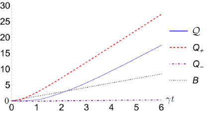
(a) $\gamma t\leq 6$

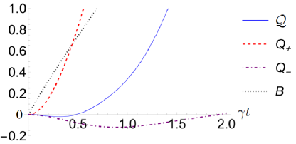
(b) $\gamma t\leq 2$

Figure 1: $\mathcal{Q}$, $Q_{+}$, $Q_{-}$, and $B$ for (a) $\gamma t\leq 6$ and (b) $\gamma t\leq 2$. The horizontal axes are $\gamma t$. We set $\Omega=\gamma$, $\Delta=0.25\gamma$, $n=1$ and $\rho(0)=\frac{1}{2}(1+0.2\sigma_{x}+0.3\sigma_{y}-0.4\sigma_{z})$. Here, $\sigma_{i}$ is the Pauli matrix ($\sigma_{y}=-i|0\rangle\langle 1|+i|1\rangle\langle 0|$, etc.).

V Quantum speed limit

In this section, we discuss a quantum speed limit derived by Hasegawa [35]:

$$\frac{1}{2}\int_{t_{1}}^{t_{2}}dt\ \sqrt{\mathcal{J}(t)}\geq D(\sigma(t_{1}),\sigma(t_{2})).$$ (54)

Here, $\sigma(t):=|\Psi_{\tau}(\tau;t)\rangle\langle\Psi_{\tau}(\tau;t)|$. (54) is the Mandelstam-Tamm relation [28, 29] applied to a state $|\Psi_{\tau}(s;t)\rangle$ defined by

$$|\Psi_{\tau}(s;t)\rangle:=V_{\tau}(s;t)|\tilde{\psi}(0)\rangle\otimes|0\rangle$$ (55)

with

$$V_{\tau}(s;t):={\rm{T}}\exp\Big{[}\int_{0}^{s}du\ \Big{\{}-i\frac{t}{\tau}H_{S}\Big{(}\frac{t}{\tau}u\Big{)}$$

$$\hskip 14.22636pt+\sqrt{\frac{t}{\tau}}\sum_{k}[L_{k}\Big{(}\frac{t}{\tau}u\Big{)}\otimes\phi_{k}^{\dagger}(u)$$

$$\hskip 48.36967pt-L_{k}\Big{(}\frac{t}{\tau}u\Big{)}^{\dagger}\otimes\phi_{k}(u)]\Big{\}}\Big{]}.$$ (56)

Here, $|\tilde{\psi}(0)\rangle$ is a purification of $\rho(0)$ (${\rm{Tr}}_{A}[|\tilde{\psi}(0)\rangle\langle\tilde{\psi}(0)|]=\rho(0)$ where $A$ is the ancilla system). ${\rm{T}}$ is the time ordering operator. $\{\phi_{k}(t)\}$ are field operators having the canonical commutation relation

$$[\phi_{k}(t),\phi_{l}^{\dagger}(s)] =\delta_{kl}\delta(t-s)$$ (57)

and $|0\rangle$ is the vacuum state for the fields. $\mathcal{J}(t)$ is the SLD Fisher information for time (see (76)):

$$\mathcal{J}(t) :=4[\langle\partial_{t}\Psi_{\tau}(\tau;t)|\partial_{t}\Psi_{\tau}(\tau;t)\rangle$$

$$-\langle\partial_{t}\Psi_{\tau}(\tau;t)|\Psi_{\tau}(\tau;t)\rangle\langle\Psi_{\tau}(\tau;t)|\partial_{t}\Psi_{\tau}(\tau;t)\rangle]$$ (58)

where $|\partial_{t}\Psi_{\tau}(\tau;t)\rangle:=\partial_{t}|\Psi_{\tau}(\tau;t)\rangle$. In Mandelstam-Tamm relation, $\mathcal{J}(t)/4$ is reduced to the energy fluctuation. In Hasegawa’s theory, the Hamiltonian becomes $i\frac{\partial V_{\tau}(\tau;t)}{\partial t}V_{\tau}(\tau;t)^{\dagger}$, which does not related to the real system dynamics and thus the physical meaning may not be so clear. $D(\rho,\sigma)$ is the Bures angle:

$$D(\rho,\sigma) :=\cos^{-1}F(\rho,\sigma),$$ (59)

$$F(\rho,\sigma) :={\rm{Tr}}\sqrt{\sqrt{\rho}\sigma\sqrt{\rho}}=F(\sigma,\rho).$$ (60)

$F(\rho,\sigma)$ is the fidelity [39]. Because of the contractivity of the Bures angle (p.414 of Ref.[39]) and $\rho(t)={\rm{Tr}}_{AB}\sigma(t)$ ($B$ is the field system),

$$D(\sigma(t_{1}),\sigma(t_{2}))\geq D(\rho(t_{1}),\rho(t_{2}))$$ (61)

holds. Note that the trace distance $T(\rho_{1},\rho_{2}):=\frac{1}{2}{\rm{Tr}}_{S}\sqrt{(\rho_{1}-\rho_{2})^{2}}$ is smaller than the Bures angle $D(\rho_{1},\rho_{2})\geq T(\rho_{1},\rho_{2})$ [39]. For time-independent $H_{S}$ and $L_{k}$, we recognize that the two SLD Fisher information (2) and (58) are connected (Appendix F)

$$\mathcal{J}(t)=\frac{\mathcal{I}(t)}{t^{2}}=\frac{B(t)+Q_{+}(t)}{t^{2}}.$$ (62)

The quantum correction $Q_{+}$ can be eliminated in the interaction picture $\tilde{\rho}(t):=e^{iH_{S}t}\rho(t)e^{-iH_{S}t}$ when

$$[L_{k},H_{S}] =\omega_{k}L_{k},$$ (63)

where $\omega_{k}$ is a real number. The quantum master equation for $\tilde{\rho}(t)$ is given by

$$\frac{d\tilde{\rho}}{dt} =\sum_{k}\Big{[}L_{k}\tilde{\rho}(t)L_{k}^{\dagger}-\frac{1}{2}\{L_{k}^{\dagger}L_{k},\tilde{\rho}(t)\}\Big{]}.$$ (64)

Repeating the arguments from (54) to (62), we obtain a quantum speed limit of the system expressed with the dynamical activity:

$$l(t_{1},t_{2}):=\frac{1}{2}\int_{t_{1}}^{t_{2}}dt\ \frac{\sqrt{B(t)}}{t}\geq D(\tilde{\rho}(t_{1}),\tilde{\rho}(t_{2})).$$ (65)

Here, $0\leq t_{1}\leq t_{2}$. (65) is the second main result of this paper.

As an instance, we consider a spinless quantum dot coupled to a single lead,

$$\frac{d\rho}{dt}=-i[H_{S},\rho]+\gamma[1-f(\varepsilon)]\mathcal{D}[a](\rho)+\gamma f(\varepsilon)\mathcal{D}[a^{\dagger}](\rho)$$ (66)

where $H_{S}=\varepsilon a^{\dagger}a$ and $\mathcal{D}[X](\bullet):=X\bullet X^{\dagger}-\frac{1}{2}\{X^{\dagger}X,\bullet\}$. Here, $a$ is the annihilation operator of the electron of the system, $\varepsilon$ is the energy level of the system, $f(\varepsilon)=\frac{1}{e^{\beta\varepsilon}+1}$ is the Fermi distribution, $\beta$ is the inverse temperature of the lead, and $\gamma$ is the coupling strength. The jump operators are $L_{1}=\sqrt{\gamma[1-f(\varepsilon)]}a$ and $L_{2}=\sqrt{\gamma f(\varepsilon)}a^{\dagger}$ with $\omega_{1}=\varepsilon$ and $\omega_{2}=-\varepsilon$. (See Appendix G for detailed calculations). Figure 2(a) shows the Bures angle $D$, the trace distance $T$, and geometric length $l$ as functions of final time $t_{2}$. In Fig.2, we set the initial time $\gamma t_{1}=2$. Figure 2(b) shows that the bound achievement ratio $D(\tilde{\rho}(t_{1}),\tilde{\rho}(t_{2}))/l(t_{1}.t_{2})$ becomes greater than 0.8 around $\gamma t_{2}=2$. In Fig.3, we showed the results when the initial time $\gamma t_{1}=0$. Around $\gamma t=0$, because of $B(t)\propto t$ and $l(0,t)\propto\sqrt{t}$, the bound achievement ratio grows in square root of time $D(\tilde{\rho}(0),\tilde{\rho}(t))/l(0,t)\propto\sqrt{t}$. The square root dependence makes the upper bound looser in the short time regime as shown in Fig.3(a).

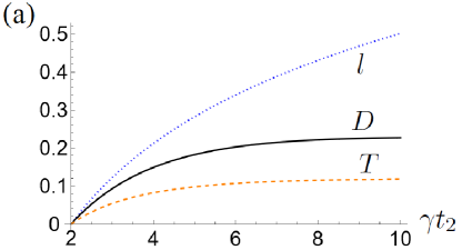
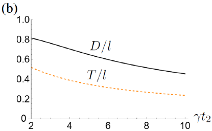
Figure 2: (a) $l(t_{1}.t_{2})$, $D(\tilde{\rho}(t_{1}),\tilde{\rho}(t_{2}))$, and $T(\tilde{\rho}(t_{1}),\tilde{\rho}(t_{2}))$, (b) $D(\tilde{\rho}(t_{1}),\tilde{\rho}(t_{2}))/l(t_{1}.t_{2})$, and $T(\tilde{\rho}(t_{1}),\tilde{\rho}(t_{2}))/l(t_{1}.t_{2})$ for $\gamma t_{1}=2$. The horizontal axes are $\gamma t_{2}$. $\beta\varepsilon=10$, $\rho(0)=\frac{1}{2}(1-0.5\sigma_{x}+0.3\sigma_{y}+0.2\sigma_{z})$. $\sigma_{i}$ is the Pauli matrix.

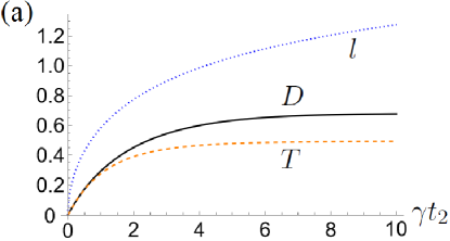
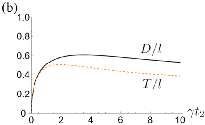
Figure 3: (a) $l(t_{1}.t_{2})$, $D(\tilde{\rho}(t_{1}),\tilde{\rho}(t_{2}))$, and $T(\tilde{\rho}(t_{1}),\tilde{\rho}(t_{2}))$, (b) $D(\tilde{\rho}(t_{1}),\tilde{\rho}(t_{2}))/l(t_{1}.t_{2})$, and $T(\tilde{\rho}(t_{1}),\tilde{\rho}(t_{2}))/l(t_{1}.t_{2})$ for $\gamma t_{1}=0$. The horizontal axes are $\gamma t_{2}$. Other parameters are same with Fig.2.

Naive extensions of (5) and (6) to the quantum regime may be,

$$\sqrt{\frac{B(\tau)\sigma}{2}} \geq T(\tilde{\rho}(0),\tilde{\rho}(\tau)),$$ (67)

$$B(\tau) \geq T(\tilde{\rho}(0),\tilde{\rho}(\tau)).$$ (68)

However, we numerically checked that they fail even in the spinless quantum dot due to the quantum effect. Actually the quantum extensions of (5) contain nontrivial quantum corrections [31, 10, 34]. However, the quantum extension of (6) has been less investigated. We speculate

$$\sqrt{B(\tau)} \geq D(\tilde{\rho}(0),\tilde{\rho}(\tau))$$ (69)

from the discussion of Fig. 3. However, from (65), we only could derive a looser bound,

$$\sqrt{b_{\rm{max}}(\tau)\tau}\geq D(\tilde{\rho}(0),\tilde{\rho}(\tau))$$ (70)

with

$$b_{\rm{max}}(\tau):=\max_{0\leq t\leq\tau}\frac{1}{t}B(t).$$ (71)

Here, we used $\sqrt{b_{\rm{max}}(\tau)\tau}\geq l(0,\tau)$. Thus (69) would be correct in the short time limit. Derivation of a simple quantum speed limit at zero initial time is a future work. The extension to the first passage time [40, 41, 42] for open quantum systems is also an interesting problem.

VI Summary

We investigated the symmetric logarithm derivative (SLD) Fisher information, which appears in the context of KUR and is the upper bound of the Fisher information of the quantum trajectory for the time-rescaling parameter. For a finite time and arbitrary initial state, we derived a concise expression of the SLD Fishder information using a double time integral, which can be calculated by numerically solving coupled first-order ordinary differential equations. We also derived a simple lower bound of the Fisher information for the probability of quantum trajectory. Furthermore, we pointed out that for time-independent system, the SLD Fisher information divided by time squared is identical to the SLD Fisher information appeared in the Mandelstam-Tamm speed limit by Hasegawa [35]. Based on this observation, we showed that when the jump operators connects energy eigenstates, the upper bound of the Bures angle between the initial and final states in the interaction picture is expressed with the square root of the dynamical activity.

Appendix A SLD Fisher information and the two-sided GKSL equation

A.1 SLD Fisher information

We consider $n$ real parameters $\theta=(\theta^{1},\cdots,\theta^{n})$ and a state $\rho^{\theta}$. The SLD $S_{i}^{\theta}$ is defined by

$$\partial_{i}\rho^{\theta} =\frac{1}{2}(\rho^{\theta}S_{i}^{\theta}+S_{i}^{\theta}\rho^{\theta}),\quad S_{i}^{\theta}=(S_{i}^{\theta})^{\dagger}.$$ (72)

Here, $\partial_{i}=\partial/\partial\theta^{i}$. Although $S_{i}^{\theta}$ is not unique in general, the SLD Fisher information matrix

$$J_{ij}^{\theta}:=\frac{1}{2}{\rm{Tr}}\Big{[}\rho^{\theta}\{S_{i}^{\theta},S_{j}^{\theta}\}\Big{]}$$ (73)

is unique [38]. $J_{ij}^{\theta}$ can be rewritten as $J_{ij}^{\theta}={\rm{Tr}}[\partial_{i}\rho^{\theta}S_{j}^{\theta}]$.

In the following, we consider a pure state $\rho^{\theta}$. Differentiating $(\rho^{\theta})^{2}=\rho^{\theta}$, we obtain

$$\partial_{i}\rho^{\theta} =(\partial_{i}\rho^{\theta})\rho^{\theta}+\rho^{\theta}\partial_{i}\rho^{\theta}.$$ (74)

Thus, $2\partial_{i}\rho^{\theta}$ is an SLD. Using this relation and denoting $\rho^{\theta}=|\psi^{\theta}\rangle\langle\psi^{\theta}|$, we obtain

$$J_{ij}^{\theta}=4{\rm{Re}}\Big{[}\langle\partial_{i}\psi^{\theta}|\partial_{j}\psi^{\theta}\rangle-\langle\partial_{i}\psi^{\theta}|\psi^{\theta}\rangle\langle\psi^{\theta}|\partial_{j}\psi^{\theta}\rangle\Big{]}.$$ (75)

Here, $|\partial_{i}\psi^{\theta}\rangle:=\partial_{i}|\psi^{\theta}\rangle$. For $n=1$, $J^{\theta}:=J_{11}^{\theta}$ becomes

$$J^{\theta}=4\big{[}\langle\partial_{\theta}\psi^{\theta}|\partial_{\theta}\psi^{\theta}\rangle-\langle\partial_{\theta}\psi^{\theta}|\psi^{\theta}\rangle\langle\psi^{\theta}|\partial_{\theta}\psi^{\theta}\rangle\big{]}.$$ (76)

A.2 Continuous measurement

We introduce $(M+1)$-dimensional Hilbert space $\mathcal{H}$ with an orthonormal basis $\{|m\rangle\}_{m=0}^{M}$ and a fictitious environment system $E$ of which Hilbert space is $\mathcal{H}^{\otimes N}$. We consider a combined system of $S$, the ancilla system $A$, and $E$. We suppose that the initial state of the combined system is $|\tilde{\psi}(0)\rangle\otimes|0_{N-1},\cdots,0_{1},0_{0}\rangle$. Here, $|\tilde{\psi}(0)\rangle$ is the purification of $\rho(0)$ (i.e. ${\rm{Tr}}_{A}[|\tilde{\psi}(0)\rangle\langle\tilde{\psi}(0)|]=\rho(0)$), and $|0_{N-1},\cdots,0_{1},0_{0}\rangle=\otimes_{i=0}^{N-1}|0\rangle_{i}$. For each $i=0,1,\cdots,N-1$, an environmental subspace $i$ interacts with system $S$ during the time interval $[i\Delta t,(i+1)\Delta t]$ via a unitary operator $U_{i}$. Here, $\Delta t:=\tau/N$. The state of the combined system at time $\tau$ is given by

$$|\psi^{\theta}\rangle =U_{N-1}\cdots U_{1}U_{0}|\tilde{\psi}(0)\rangle\otimes|0_{N-1},\cdots,0_{1},0_{0}\rangle$$

$$=\sum_{m_{0},\cdots,m_{N-1}=0}^{M}\Omega_{m_{N-1}}^{\theta}\cdots\Omega_{m_{0}}^{\theta}|\tilde{\psi}(0)\rangle$$

$$\hskip 76.82243pt\otimes|m_{N-1},\cdots,m_{1},m_{0}\rangle$$ (77)

where $\Omega_{m_{i}}^{\theta}$ is defined by

$$\langle k_{S}|\Omega_{m_{i}}^{\theta}|k_{S}^{\prime}\rangle =\langle k_{S}|{}_{i}\langle m_{i}|U_{i}|k_{S}^{\prime}\rangle|0\rangle_{i}.$$ (78)

$|k_{S}\rangle$ and $|k_{S}^{\prime}\rangle$ are bases of the system. We suppose that $\Omega_{m}^{\theta}$ are the same as (17) and (18). The Fisher information associated with POVM (positive operator valued measure) [39] $\mathcal{M}$ is denoted by $I(\theta,\mathcal{M})$. If we put $\mathcal{M}_{0}(\{m_{i}\}):=1_{SA}\otimes|m_{N-1},\cdots,m_{1},m_{0}\rangle\langle m_{N-1},\cdots,m_{1},m_{0}|$ ($1_{SA}$ is the identity operator of $SA$), the outcome is given by

$${\rm{Tr}}[\mathcal{M}_{0}(\{m_{i}\})|\psi^{\theta}\rangle\langle\psi^{\theta}|]=P^{\theta}(\{m_{i}\}).$$ (79)

Thus, $\tilde{F}$ defined by (20) is given by

$$\tilde{F} =I(0,\mathcal{M}_{0}(\{m_{i}\})).$$ (80)

Because of the quantum Cramér-Rao theorem [37, 38],

$$I(\theta,\mathcal{M})\leq J^{\theta}$$ (81)

holds. Here, $J^{\theta}$ is the SLD Fisher information given by (76). Using (80), (81) and (76), we obtain

$$F \leq\mathcal{I}=4\Big{[}\frac{\partial^{2}}{\partial\theta_{1}\partial\theta_{2}}\langle\psi^{\theta_{2}}|\psi^{\theta_{1}}\rangle$$

$$\quad-\Big{(}\frac{\partial}{\partial\theta_{2}}\langle\psi^{\theta_{2}}|\psi^{\theta_{1}}\rangle\Big{)}\Big{(}\frac{\partial}{\partial\theta_{1}}\langle\psi^{\theta_{2}}|\psi^{\theta_{1}}\rangle\Big{)}\Big{]}\Big{|}_{\theta_{1}=0=\theta_{2}}.$$ (82)

Here,

$$\langle\psi^{\theta_{2}}|\psi^{\theta_{1}}\rangle ={\rm{Tr}}_{S}\rho^{\theta_{1},\theta_{2}}(\tau),$$ (83)

$$\rho^{\theta_{1},\theta_{2}}(\tau) :={\rm{Tr}}_{AE}[|\psi^{\theta_{1}}\rangle\langle\psi^{\theta_{2}}|].$$ (84)

The time evolution equation of $\rho^{\theta_{1},\theta_{2}}(t)$ is given by (15) [26]. Then, we obtain (14).

To obtain (22), we adopt a purification

$$|\tilde{\psi}(0)\rangle=\sum_{\alpha}\sqrt{p_{\alpha}}|\alpha\rangle\otimes|\varphi_{\alpha}\rangle_{A}$$ (85)

with ${}_{A}\langle\varphi_{\alpha}|\varphi_{\beta}\rangle_{A}=\delta_{\alpha\beta}$ and the POVM $\mathcal{M}_{0}(\alpha,\{m_{i}\}):=|\varphi_{\alpha}\rangle_{A}{}_{A}\langle\varphi_{\alpha}|\otimes|m_{N-1},\cdots,m_{1},m_{0}\rangle\langle m_{N-1},\cdots,m_{1},m_{0}|$. Then the outcomes becomes (22):

$${\rm{Tr}}[\mathcal{M}_{0}(\alpha,\{m_{i}\})|\psi^{\theta}\rangle\langle\psi^{\theta}|]=P^{\theta}(\alpha,\{m_{i}\}).$$ (86)

The associated Fisher information defined by (23) is given by

$$\tilde{F}^{\prime} =I(0,\mathcal{M}_{0}(\alpha,\{m_{i}\})).$$ (87)

Then, $F^{\prime}\leq\mathcal{I}$ holds.

Appendix B Derivation of (31)

In the following, we use the Liouville space. An arbitrary linear operator $X$ of the system is described by a vector $|X\rangle\rangle$. The inner product is defined by $\langle\langle Y|X\rangle\rangle:={\rm{Tr}}_{S}(Y^{\dagger}X)$. In particular, $\langle\langle 1|X\rangle\rangle={\rm{Tr}}_{S}(X)$. An arbitrary linear super-operator of the system is described by an operator of Liouville space. The conservation of the probability leads to $\langle\langle 1|\mathcal{L}(t)=0$.

$\mathcal{C}(\theta_{1},\theta_{2})$ is given by

$$\mathcal{C}(\theta_{1},\theta_{2}) =\langle\langle 1|\mathcal{U}^{\theta_{1},\theta_{2}}(\tau,0)|\rho(0)\rangle\rangle$$ (88)

where $\mathcal{U}^{\theta_{1},\theta_{2}}(u,s)$ is defined by

$$\frac{\partial\mathcal{U}^{\theta_{1},\theta_{2}}(u,s)}{\partial u} =\mathcal{L}^{\theta_{1},\theta_{2}}(u)\mathcal{U}^{\theta_{1},\theta_{2}}(u,s)$$ (89)

with $\mathcal{U}^{\theta_{1},\theta_{2}}(s,s)=1$. Note that $\mathcal{U}^{0,0}(u,s)=\mathcal{U}(u,s)$. The first derivative leads to

$$\partial_{\theta_{i}}\mathcal{C}(\theta_{1},\theta_{2}) =\int_{0}^{\tau}du\ \langle\langle 1|\mathcal{U}^{\theta_{1},\theta_{2}}(\tau,u)\partial_{\theta_{i}}\mathcal{L}^{\theta_{1},\theta_{2}}(u)$$

$$\hskip 14.22636pt\times\mathcal{U}^{\theta_{1},\theta_{2}}(u,0)|\rho(0)\rangle\rangle\ \ (i=1,2).$$ (90)

Using the above equation, $\mathcal{U}^{0,0}(s,0)|\rho(0)\rangle\rangle=|\rho(s)\rangle\rangle$, and

$$\langle\langle 1|\mathcal{U}^{0,0}(s,0) =\langle\langle 1|,$$ (91)

we obtain (36). (91) is derived from $\langle\langle 1|\mathcal{L}(s)=0$. The second derivative (31) consists of

$$\int_{0}^{\tau}ds\ {\rm{Tr}}_{S}\Big{[}\partial_{\theta_{1}}\partial_{\theta_{2}}\mathcal{L}^{\theta_{1},\theta_{2}}(s)\big{|}_{\theta_{1}=0=\theta_{2}}\rho(s)\Big{]}=\frac{1}{4}B(\tau)$$ (92)

and

$$\int_{0}^{\tau}ds\int_{0}^{s}du\ {\rm{Tr}}_{S}\Big{[}\partial_{\theta_{i^{\prime}}}\mathcal{L}^{\theta_{1},\theta_{2}}(s)\mathcal{U}^{\theta_{1},\theta_{2}}(s,u)$$

$$\hskip 14.22636pt\times\partial_{\theta_{i}}\mathcal{L}^{\theta_{1},\theta_{2}}(u)\big{|}_{\theta_{1}=0=\theta_{2}}\rho(u)\Big{]}=I_{i}\ \ (i=1,2)$$ (93)

with $1^{\prime}:=2$ and $2^{\prime}:=1$. Note that

$$\mathcal{L}_{i}(s)=\partial_{\theta_{i}}\mathcal{L}^{\theta_{1},\theta_{2}}(s)\big{|}_{\theta_{1}=0=\theta_{2}}.$$ (94)

$Q_{+}(t)$ can be written as

$$Q_{+}(t) =Q_{a}(t)+Q_{b}(t),$$ (95)

where

$$Q_{b}(t)$$

$$:=4\int_{0}^{t}ds\int_{0}^{s}du\ {\rm{Tr}}_{S}\Big{[}\mathcal{L}_{1}(t)\mathcal{U}(s,u)\mathcal{P}(u)\mathcal{L}_{2}(u)\rho(u)\Big{]}.$$ (96)

$q_{a}$ in (43) is defined by

$$q_{a}(s):=\int_{0}^{s}du\ \mathcal{U}(s,u)\mathcal{P}(u)\mathcal{L}_{1}(u)\rho(u).$$ (97)

Because of

$$(\mathcal{L}\bullet)^{\dagger} =\mathcal{L}\bullet^{\dagger},$$ (98)

$$(\mathcal{L}_{i}\bullet)^{\dagger} =\mathcal{L}_{i^{\prime}}\bullet^{\dagger},$$ (99)

$$(\mathcal{P}\mathcal{L}_{i}\bullet)^{\dagger} =\mathcal{P}\mathcal{L}_{i^{\prime}}\bullet^{\dagger},$$ (100)

$Q_{b}=Q_{a}^{\ast}$ holds. Then, we obtain (40)

Appendix C Quantum correction $Q_{+}$ in the long-time region

The left and right eigenvalue equations of the Liouvillian $\mathcal{L}$ are

$$\mathcal{L}|\rho_{n}\rangle\rangle =\lambda_{n}|\rho_{n}\rangle\rangle,$$ (101)

$$\langle\langle l_{n}|\mathcal{L} =\lambda_{n}\langle\langle l_{n}|.$$ (102)

We set $\langle\langle l_{m}|\rho_{n}\rangle\rangle=\delta_{mn}$, $\lambda_{0}=0$, and $\langle\langle l_{0}|=\langle\langle 1|$. Then, $\rho_{0}(=:\rho^{\rm{ss}})$ is the steady state.

If the initial state is the steady state, (95) becomes

$$Q_{+}(\tau) =4\Big{(}\int_{0}^{\tau}ds\int_{0}^{s}du\ {\rm{Tr}}_{S}\Big{[}\mathcal{L}_{2}e^{(s-u)\mathcal{L}}\mathcal{P}\mathcal{L}_{1}\rho^{\rm{ss}}\Big{]}$$

$$\quad+\int_{0}^{\tau}ds\int_{0}^{s}du\ {\rm{Tr}}_{S}\Big{[}\mathcal{L}_{1}e^{(s-u)\mathcal{L}}\mathcal{P}\mathcal{L}_{2}\rho^{\rm{ss}}\Big{]}\Big{)}$$ (103)

with

$$\mathcal{P}:=1-|\rho^{\rm{ss}}\rangle\rangle\langle\langle 1|.$$ (104)

Using

$$e^{(s-u)\mathcal{L}} =\sum_{n}e^{(s-u)\lambda_{n}}|\rho_{n}\rangle\rangle\langle\langle l_{n}|,$$ (105)

we obtain

$$\int_{0}^{\tau}ds\int_{0}^{s}du\ e^{(s-u)\mathcal{L}}\mathcal{P}$$

$$=\sum_{n\neq 0}\int_{0}^{\tau}ds\int_{0}^{s}du\ e^{(s-u)\lambda_{n}}\mathcal{P}|\rho_{n}\rangle\rangle\langle\langle l_{n}|$$

$$=-\tau\sum_{n\neq 0}\frac{1}{\lambda_{n}}|\rho_{n}\rangle\rangle\langle\langle l_{n}|-\sum_{n\neq 0}\frac{1}{\lambda_{n}^{2}}|\rho_{n}\rangle\rangle\langle\langle l_{n}|$$

$$\quad+\sum_{n\neq 0}\frac{e^{\tau\lambda_{n}}}{\lambda_{n}^{2}}|\rho_{n}\rangle\rangle\langle\langle l_{n}|$$

$$\approx-\tau\sum_{n\neq 0}\frac{1}{\lambda_{n}}|\rho_{n}\rangle\rangle\langle\langle l_{n}|=-\tau\mathcal{R},$$ (106)

where

$$\mathcal{R} :=\sum_{n\neq 0}\frac{1}{\lambda_{n}}|\rho_{n}\rangle\rangle\langle\langle l_{n}|=-\int_{0}^{\infty}dt\ e^{t\mathcal{L}}\mathcal{P}$$ (107)

is the pseudo-inverse of the Liouvillian [22, 43, 44, 45, 46, 47] (the Drazin inverse [48] of $\mathcal{L}$). Thus, we obtain

$$Q_{+}(\tau)\approx-4\tau\Big{(}{\rm{Tr}}_{S}\Big{[}\mathcal{L}_{2}\mathcal{R}\mathcal{L}_{1}\rho^{\rm{ss}}\Big{]}+{\rm{Tr}}_{S}\Big{[}\mathcal{L}_{1}\mathcal{R}\mathcal{L}_{2}\rho^{\rm{ss}}\Big{]}\Big{)}$$ (108)

in the long-time limit. The expression of $Q_{+}$ in the long-time approximation is consistent with (28).

Appendix D Lower bound of $\mathcal{Q}$

(20) can be rewritten as

$$\tilde{F}=\sum_{m_{0},\cdots,m_{N-1}=0}^{M}P^{0}(\{m_{i}\})\Big{[}\partial_{\theta}\ln P^{\theta}(\{m_{i}\})\big{|}_{\theta=0}\Big{]}^{2}.$$ (109)

The score $\partial_{\theta}\ln P^{\theta}(\{m_{i}\})|_{\theta=0}$ is given by

$$\partial_{\theta}\ln P^{\theta}(\{m_{i}\})|_{\theta=0}=b(\{m_{i}\})+d(\{m_{i}\})$$ (110)

where

$$b(\{m_{i}\}) :=\sum_{n=0}^{N-1}\delta_{m_{n}\neq 0},$$ (111)

$$d(\{m_{i}\}) :=\sum_{n=0}^{N-1}\delta_{m_{n},0}\gamma_{n}(\{m_{i}\})\Delta t,$$ (112)

$$\gamma_{n}(\{m_{i}\}) :=\frac{{\rm{Tr}}_{S}[\hat{\Omega}_{m_{N-1}}\cdots\hat{\gamma}\cdots\hat{\Omega}_{m_{0}}\rho(0)]}{P^{0}(\{m_{i}\})}.$$ (113)

Here we introduce the convention that $\delta_{m\neq 0}:=1-\delta_{m,0}$ and $\hat{\Omega}_{m}\bullet:=\Omega_{m}^{0}\bullet(\Omega_{m}^{0})^{\dagger}$. $\hat{\gamma}$ is defined by (46). Then $\tilde{F}$ becomes

$$\tilde{F} =\langle b(\{m_{i}\})^{2}\rangle+2\langle b(\{m_{i}\})d(\{m_{i}\})\rangle+\langle d(\{m_{i}\})^{2}\rangle$$ (114)

where $\langle X(\{m_{i}\})\rangle:=\sum_{m_{0},\cdots,m_{N-1}=0}^{M}P^{0}(\{m_{i}\})X(\{m_{i}\})$. $b(\{m_{i}\})^{2}$ and $b(\{m_{i}\})d(\{m_{i}\})$ are calculated as

$$b(\{m_{i}\})^{2} =b(\{m_{i}\})+2\sum_{n=1}^{N-1}\sum_{l=0}^{n-1}\delta_{m_{n}\neq 0}\delta_{m_{l}\neq 0},$$ (115)

and

$$b(\{m_{i}\})d(\{m_{i}\}) =\sum_{n=1}^{N-1}\sum_{l=0}^{n-1}\Big{(}\delta_{m_{n}\neq 0}\gamma_{l}(\{m_{i}\})\delta_{m_{l},0}\Delta t$$

$$\quad+\gamma_{n}(\{m_{i}\})\delta_{m_{n},0}\Delta t\delta_{m_{l}\neq 0}\Big{)}.$$ (116)

In (115), the first and second terms of the right-hand side come from the contributions of the same times and different times respectively. In the limit of $\Delta t\to 0$, trajectory averages of the above two equations become

$$\langle b(\{m_{i}\})^{2}\rangle=B(\tau)$$

$$\quad+2\int_{0}^{\tau}ds\int_{0}^{s}du\ {\rm{Tr}}_{S}[\hat{\Gamma}(s)\mathcal{U}(s,u)\hat{\Gamma}(u)\rho(u)],$$ (117)

$$\langle b(\{m_{i}\})d(\{m_{i}\})\rangle$$

$$=\int_{0}^{\tau}ds\int_{0}^{s}du\ \Big{(}{\rm{Tr}}_{S}[\hat{\Gamma}(s)\mathcal{U}(s,u)\hat{\gamma}(u)\rho(u)]$$

$$\quad+{\rm{Tr}}_{S}[\hat{\gamma}(s)\mathcal{U}(s,u)\hat{\Gamma}(u)\rho(u)]\Big{)}$$ (118)

where $\hat{\Gamma}(t)\bullet:=\sum_{k}L_{k}\bullet L_{k}^{\dagger}$. Thus, we obtain

$$\langle b(\{m_{i}\})^{2}\rangle+2\langle b(\{m_{i}\})d(\{m_{i}\})\rangle$$

$$=B(\tau)-2\int_{0}^{\tau}ds\int_{0}^{s}du\ {\rm{Tr}}_{S}[\hat{\gamma}(s)\mathcal{U}(s,u)\hat{\gamma}(u)\rho(u)]$$ (119)

and

$$\mathcal{Q}=\langle d(\{m_{i}\})^{2}\rangle$$

$$\quad-2\int_{0}^{\tau}ds\int_{0}^{s}du\ {\rm{Tr}}_{S}[\hat{\gamma}(s)\mathcal{U}(s,u)\hat{\gamma}(u)\rho(u)].$$ (120)

Here, $\langle d(\{m_{i}\})^{2}\rangle$ cannot be written as the double time integral because $\gamma_{n}(\{m_{i}\})$ in $d(\{m_{i}\})$ depends on the entire sequence of a trajectory $\{m_{i}\}$. Using $\langle d(\{m_{i}\})^{2}\rangle\geq\langle d(\{m_{i}\})\rangle^{2}$, $\langle b(\{m_{i}\})+d(\{m_{i}\})\rangle=0$, and $\langle b(\{m_{i}\})\rangle=B(\tau)$, we obtain (45).

Appendix E Derivations of (50) and (51)

We start from (25). We suppose that the matrix representation of $\mathcal{L}^{\theta_{1},\theta_{2}}$ is block diagonalized, with one block $\tilde{\mathcal{L}}^{\theta_{1},\theta_{2}}$ having eigenvalue $\lambda(\theta_{1},\theta_{2})$. The characteristic polynomial of $\tilde{\mathcal{L}}^{\theta_{1},\theta_{2}}$ is given by

$$\det(\tilde{\mathcal{L}}^{\theta_{1},\theta_{2}}-\lambda 1_{d})=\sum_{n=0}^{d}a^{(n)}(\theta_{1},\theta_{2})\lambda^{n}.$$ (121)

Here, $d$ is the dimension of $\tilde{\mathcal{L}}^{\theta_{1},\theta_{2}}$ and $1_{d}$ is $d$-dimensional identity matrix. By differentiating $\sum_{n=0}^{d}a^{(n)}(\theta_{1},\theta_{2})\lambda(\theta_{1},\theta_{2})^{n}=0$, we obtain

$$a^{(0)}_{i}+a^{(1)}\lambda_{i}=0\ \ (i=1,2),$$ (122)

$$a^{(0)}_{12}+a^{(1)}\lambda_{12}+a^{(1)}_{1}\lambda_{2}+a^{(1)}_{2}\lambda_{1}+2a^{(2)}\lambda_{1}\lambda_{2}=0.$$ (123)

Here, $a^{(n)}:=a^{(n)}(0,0)$, $X_{i}:=\partial_{\theta_{i}}X|_{\theta_{1}=0=\theta_{2}}$, and $X_{12}:=\partial_{\theta_{1}}\partial_{\theta_{2}}X|_{\theta_{1}=0=\theta_{2}}$. $\lambda_{12}$ is calculated from (122) and (123). $\dot{Q}_{+}:=\lim_{\tau\to\infty}Q_{+}/\tau$ is given by

$$\dot{Q}_{+} =4\lambda_{12}-{\color[rgb]{0,0,0}\dot{B}_{\rm{ss}}}.$$ (124)

For the system described by (47)-(49), $\tilde{\mathcal{L}}^{\theta_{1},\theta_{2}}$ is given by

$$\tilde{\mathcal{L}}^{\theta_{1},\theta_{2}}$$

$$=\begin{pmatrix}-\frac{1}{2}(\Theta_{1}+\Theta_{2})\gamma n&i\Theta_{2}\Omega&-\Theta_{1}\Omega&\sqrt{\Theta_{1}\Theta_{2}}\gamma(n+1)\\ i\Theta_{2}\Omega&i\Theta_{2}\Delta-\frac{1}{2}\Theta_{2}\gamma(n+1)-\frac{1}{2}\Theta_{1}\gamma n&0&-i\Theta_{1}\Omega\\ -i\Theta_{1}\Omega&0&-i\Theta_{1}\Delta-\frac{1}{2}\Theta_{1}\gamma(n+1)-\frac{1}{2}\Theta_{2}\gamma n&i\Theta_{2}\Omega\\ \sqrt{\Theta_{1}\Theta_{2}}\gamma n&-i\Theta_{1}\Omega&i\Theta_{2}\Omega&\mathcal{L}_{44}\end{pmatrix}$$ (125)

with $\mathcal{L}_{44}:=-\frac{1}{2}(\Theta_{1}+\Theta_{2})\gamma(n+1)-i(\Theta_{1}-\Theta_{2})\Delta$ and $\Theta_{i}:=1+\theta_{i}$. Using (122), (123), and (124), we obtain (50).

$Q_{-}$ can be rewritten as

$$Q_{-}(t) =\frac{\partial^{2}}{\partial\theta^{2}}\ln{\rm{Tr}}_{S}\rho^{\theta}(t)\Big{|}_{\theta=0}.$$ (126)

Here, $\rho^{\theta}(t)$ is defined by

$$\frac{d}{dt}\rho^{\theta}(t) =\mathcal{L}^{\theta}\rho^{\theta}(t),$$ (127)

$$\mathcal{L}^{\theta}\bullet :=(1+i\theta)\hat{\gamma}\bullet+\sum_{k}L_{k}\bullet L_{k}^{\dagger}$$ (128)

with $\rho^{\theta}(0)=\rho(0)$. From (126), we obtain

$$Q_{-}(\tau) =\tau\frac{\partial^{2}}{\partial\theta^{2}}\Lambda(\theta)\Big{|}_{\theta=0}+O(1)$$ (129)

where $\Lambda(\theta)$ is the eigenvalue of $\mathcal{L}^{\theta}$ which satisfies $\Lambda(0)=0$. $\dot{Q}_{-}=\partial^{2}\Lambda(\theta)/\partial\theta^{2}|_{\theta=0}$ is calculated in the similar way as $\lambda_{12}$. Then, we obtain (51).

Appendix F Hasegawa’s approach

We review Hasegawa’s method and results [35]. We introduce a state

$$|\Phi(t)\rangle =U(t)|\Phi(0)\rangle$$ (130)

with

$$|\Phi(0)\rangle :=|\tilde{\psi}(0)\rangle\otimes|0\rangle,$$ (131)

$$U(t) ={\rm{T}}\exp\Big{[}\int_{0}^{t}ds\ \Big{\{}-iH_{S}(s)$$

$$+\sum_{k}[L_{k}(s)\otimes\phi_{k}^{\dagger}(s)-L_{k}(s)^{\dagger}\otimes\phi_{k}(s)]\Big{\}}\Big{]}.$$ (132)

The state $|\Phi(t)\rangle$ provides the solution of the GKSL equation [35]:

$$\rho(t) ={\rm{Tr}}_{AB}[|\Phi(t)\rangle\langle\Phi(t)|].$$ (133)

Using $d\rho={\rm{Tr}}_{AB}\big{[}d(|\Phi(t)\rangle\langle\Phi(t)|)\big{]}$,

$$d(|\Phi(t)\rangle\langle\Phi(t)|) =d|\Phi(t)\rangle\langle\Phi(t)|+|\Phi(t)\rangle d\langle\Phi(t)|$$

$$\quad+d|\Phi(t)\rangle d\langle\Phi(t)|,$$ (134)

and

$$d|\Phi(t)\rangle =\Big{(}\big{(}-iH_{S}-\frac{1}{2}\sum_{k}L_{k}^{\dagger}L_{k}\big{)}dt+\sum_{k}L_{k}d\phi_{k}^{\dagger}$$

$$\quad+\frac{1}{2}\sum_{k,l}L_{k}L_{l}d\phi_{k}^{\dagger}d\phi_{l}^{\dagger}\Big{)}|\Phi(t)\rangle,$$ (135)

we obtain the GKSL equation (7). Here, $d\phi_{k}^{\dagger}=\int_{t}^{t+dt}ds\ \phi_{k}^{\dagger}(s)$.

If we put

$$\rho_{\tau}(s;t_{1},t_{2}) :={\rm{Tr}}_{AB}[|\Psi_{\tau}(s;t_{1})\rangle\langle\Psi_{\tau}(s;t_{2})|],$$ (136)

we obtain $\rho_{\tau}(\tau;t,t)=\rho(t)$ [35]. The time evolution equation of $\rho_{\tau}(s;t_{1},t_{2})$ is given by

$$\frac{\partial\rho_{\tau}(s;t_{1},t_{2})}{\partial s} =\mathcal{L}_{\tau}(s;t_{1},t_{2})\rho_{\tau}(s;t_{1},t_{2})$$ (137)

with

$$\mathcal{L}_{\tau}(s;t_{1},t_{2})\bullet$$

$$=-i\frac{t_{1}}{\tau}H_{S}\Big{(}\frac{t_{1}}{\tau}s\Big{)}\bullet+\bullet i\frac{t_{2}}{\tau}H_{S}\Big{(}\frac{t_{2}}{\tau}s\Big{)}$$

$$\quad+\sqrt{\frac{t_{1}}{\tau}}\sqrt{\frac{t_{2}}{\tau}}\sum_{k}L_{k}\Big{(}\frac{t_{1}}{\tau}s\Big{)}\bullet L_{k}\Big{(}\frac{t_{2}}{\tau}s\Big{)}^{\dagger}$$

$$\quad-\frac{1}{2}\sum_{k}\Big{[}\frac{t_{1}}{\tau}L_{k}\Big{(}\frac{t_{1}}{\tau}s\Big{)}^{\dagger}L_{k}\Big{(}\frac{t_{1}}{\tau}s\Big{)}\bullet$$

$$\hskip 34.1433pt+\bullet\frac{t_{2}}{\tau}L_{k}\Big{(}\frac{t_{2}}{\tau}s\Big{)}^{\dagger}L_{k}\Big{(}\frac{t_{2}}{\tau}s\Big{)}\Big{]}.$$ (138)

(137) is a two-sided GKSL equation. Because of

$$\mathcal{L}_{\tau}(s;t,t) =\frac{t}{\tau}\mathcal{L}\Big{(}\frac{t}{\tau}s\Big{)},$$ (139)

we obtain

$$\rho_{\tau}(s;t,t) =\rho\Big{(}\frac{t}{\tau}s\Big{)}.$$ (140)

$\mathcal{J}(t)$ defined by (58) is given by

$$\mathcal{J}(t) =4[\partial_{t_{1}}\partial_{t_{2}}C(t_{1},t_{2})$$

$$\quad-\partial_{t_{1}}C(t_{1},t_{2})\partial_{t_{2}}C(t_{1},t_{2})\Big{]}\Big{|}_{t_{1}=t=t_{2}}$$ (141)

with $C(t_{1},t_{2}):={\rm{Tr}}_{S}\rho_{\tau}(\tau;t_{1},t_{2})$. $\mathcal{J}(t)$ is independent from $\tau$.

From (54), Hasegawa [35] showed a KUR:

$$\frac{\tau^{2}(\partial_{\tau}\langle\mathcal{C}\rangle_{\tau})^{2}}{\langle\mathcal{C}^{2}\rangle_{\tau}-\langle\mathcal{C}\rangle_{\tau}^{2}}\leq\mathcal{B}(\tau).$$ (142)

Here,

$$\mathcal{B}(t):=t^{2}\mathcal{J}(t)$$ (143)

is “the quantum generalization of the dynamical activity”. $\langle X\rangle_{\tau}:=\langle\Psi_{\tau}(\tau;\tau)|X|\Psi_{\tau}(\tau;\tau)\rangle=\langle\Phi(\tau)|X|\Phi(\tau)\rangle$ and $\mathcal{C}$ is an operator of the field system which describes a time-integrated counting observable: $\mathcal{C}$ counts and weights jump events in a quantum trajectory of the system $S$. In Ref.[35], Hasegawa showed a KUR for more general operators of the field system.

If $H_{S}$ and $L_{k}$ are time-independent, (138) is obtained by replacing $1+\theta_{i}$ by $t_{i}/\tau$ ($i=1,2$) in (16). In this case, $\mathcal{B}(\tau)$ in Ref.[35] is identical to $\mathcal{I}$ in Ref.[27]:

$$\mathcal{B}(\tau)=\mathcal{I}.$$ (144)

(142) is consistent with (1).

Appendix G Quantum dot

We consider the quantum dot (66). The state of the system can be written as $\tilde{\rho}(t)=\frac{1}{2}(1+\bm{r}(t)\cdot\bm{\sigma})$. Here, $\bm{\sigma}=(\sigma_{x},\sigma_{y},\sigma_{z})$, $\sigma_{i}$ is the Pauli matrix, and $\bm{r}(t)=(x,y,z)$ is the Bloch vector. The equation of the motion of the Bloch vector is given by

$$\frac{d}{dt}x =-\frac{1}{2}\gamma x,\quad\frac{d}{dt}y=-\frac{1}{2}\gamma y,$$ (145)

$$\frac{d}{dt}z =-\gamma(z-[1-2f(\varepsilon)]).$$ (146)

The dynamical activity is given by

$$B(t)=\int_{0}^{t}ds\ \frac{\gamma}{2}\big{(}1+[2f(\varepsilon)-1]z(s)\big{)}.$$ (147)

We put $\rho_{i}:=\tilde{\rho}(t_{i})$. If the eigenvalues of $\kappa:=\sqrt{\rho_{1}}\rho_{2}\sqrt{\rho_{1}}$ are $\lambda_{1}$ and $\lambda_{2}$, the fidelity is given by $F(\rho_{1},\rho_{2})=\sqrt{\lambda_{1}}+\sqrt{\lambda_{2}}$. Then,

$$[F(\rho_{1},\rho_{2})]^{2} ={\rm{Tr}}_{S}(\kappa)+2\sqrt{\det(\kappa)}$$

$$={\rm{Tr}}_{S}(\rho_{1}\rho_{2})+2\sqrt{\det(\rho_{1})\det(\rho_{2})}.$$ (148)

This leads to

$$F(\tilde{\rho}(t_{1}),\tilde{\rho}(t_{2}))$$

$$=\sqrt{\frac{1+\bm{r}(t_{1})\cdot\bm{r}(t_{2})+\sqrt{[1-\bm{r}(t_{1})^{2}][1-\bm{r}(t_{2})^{2}]}}{2}}.$$ (149)

The Bures angle is given by $D(\tilde{\rho}(t_{1}),\tilde{\rho}(t_{2}))=\cos^{-1}F(\tilde{\rho}(t_{1}),\tilde{\rho}(t_{2}))$. The trace distance is given by

$$T(\tilde{\rho}(t_{1}),\tilde{\rho}(t_{2}))=\frac{1}{2}|\bm{r}(t_{1})-\bm{r}(t_{2})|.$$ (150)

Here, $|\bm{x}|=\sqrt{\bm{x}^{2}}=\sqrt{\bm{x}\cdot\bm{x}}$.

References

- [1] A. C. Barato and U. Seifert, “Thermodynamic Uncertainty Relation for Biomolecular Processes”, Phys. Rev. Lett. 114, 158101 (2015).
- [2] T. R. Gingrich, J. M. Horowitz, N. Perunov, and J. L. England, “Dissipation Bounds All Steady-State Current Fluctuations”, Phys. Rev. Lett. 116, 120601 (2016).
- [3] A. Dechant, and S.-i. Sasa, “Current fluctuations and transport efficiency for general Langevin systems”, J. Stat. Mech.: Theory Exp. 2018, 063209.
- [4] K. Liu, Z. Gong, and M. Ueda, “Thermodynamic Uncertainty Relation for Arbitrary Initial States”, Phys. Rev. Lett. 125, 140602 (2020).
- [5] T. Koyuk and U. Seifert, “Thermodynamic Uncertainty Relation for Time-Dependent Driving”, Phys. Rev. Lett. 125, 260604 (2020).
- [6] A. Dechant and S.-i. Sasa, “Continuous time reversal and equality in the thermodynamic uncertainty relation”, Phys. Rev. Research 3, L042012 (2021).
- [7] N. Shiraishi, “Optimal Thermodynamic Uncertainty Relation in Markov Jump Processes”, J. Stat. Phys. 185, 19 (2021).
- [8] V. T. Vo, T. V. Vu, and Y. Hasegawa, “Unified thermodynamic-kinetic uncertainty relation”, J. Phys. A: Math. Theor. 55, 405004 (2022).
- [9] K. Yoshimura, A. Kolchinsky, A. Dechant, and S. Ito, “Housekeeping and excess entropy production for general nonlinear dynamics”, Phys. Rev. Research 5, 013017 (2023).
- [10] T. V. Vu and K. Saito, “Thermodynamic Unification of Optimal Transport: Thermodynamic Uncertainty Relation, Minimum Dissipation, and Thermodynamic Speed Limits”, Phys. Rev. X 13, 011013 (2023).
- [11] J. P. Garrahan, “Simple bounds on fluctuations and uncertainty relations for first-passage times of counting observables”, Phys. Rev. E 95, 032134 (2017).
- [12] I. D. Terlizzi and M. Baiesi, “Kinetic uncertainty relation”, Journal of Physics A: Mathematical and Theoretical 52, 02LT03 (2018).
- [13] K. Hiura and S.-i. Sasa, “Kinetic uncertainty relation on first-passage time for accumulated current”, Phys. Rev. E 103, L050103 (2021).
- [14] K. Ptaszyński, “Coherence-enhanced constancy of a quantum thermoelectric generator”, Phys. Rev. B 98, 085425 (2018).
- [15] L. M. Cangemi, V. Cataudella, G. Benenti, M. Sassetti, and G. De Filippis, “Violation of thermodynamics uncertainty relations in a periodically driven work-to-work converter from weak to strong dissipation”, Phys. Rev. B 102, 165418 (2020).
- [16] A. Rignon-Bret, G. Guarnieri, J. Goold, and M. T. Mitchison, “Thermodynamics of precision in quantum nanomachines”, Phys. Rev. E 103. 012133 (2021).
- [17] A. A. S. Kalaee, A. Wacker, and P. P. Potts, “Violating the thermodynamic uncertainty relation in the three-level maser”, Phys. Rev. E 104, L012103 (2021).
- [18] P. Menczel, E. Loisa, K. Brandner, and C. Flindt, “Thermodynamic uncertainty relations for coherently driven open quantum systems”, J. Phys. A: Math. Theor. 54, 314002 (2021).
- [19] P. Bayona-Pena and K. Takahashi, “Thermodynamics of a continuous quantum heat engine: Interplay between population and coherence”, Phys. Rev. A 104, 042203 (2021).
- [20] F. Carollo, R. L. Jack, and J. P. Garrahan, “Unraveling the Large Deviation Statistics of Markovian Open Quantum Systems”, Phys. Rev. Lett. 122, 130605 (2019).
- [21] G. Guarnieri, G. T. Landi, S. R. Clark, and John Goold, “Thermodynamics of precision in quantum nonequilibrium steady states”, Phys. Rev. Research 1, 033021 (2019).
- [22] H. J. D. Miller, M. H. Mohammady. M. Perarnau-Llobet, and G. Guarnieri, “Thermodynamic Uncertainty Relation in Slowly Driven Quantum Heat Engines”, Phys. Rev. Lett. 126, 210603 (2021).
- [23] Y. Hasegawa, “Quantum Thermodynamic Uncertainty Relation for Continuous Measurement”, Phys. Rev. Lett. 125, 050601 (2020).
- [24] Y. Hasegawa, “Thermodynamic Uncertainty Relation for General Open Quantum Systems”, Phys. Rev. Lett. 126, 010602 (2021).
- [25] Y. Hasegawa, “Irreversibility, Loschmidt Echo, and Thermodynamic Uncertainty Relation”, Phys. Rev. Lett. 127, 240602 (2021).
- [26] S. Gammelmark and K. Mølmer, “Fisher Information and the Quantum Cramér-Rao Sensitivity Limit of Continuous Measurements”, Phys. Rev. Lett. 112, 170401 (2014).
- [27] T. V. Vu and K. Saito, “Thermodynamics of Precision in Markovian Open Quantum Dynamics”, Phys. Rev. Lett. 128, 140602 (2022).
- [28] L. Mandelstam and I. Tamm, “The uncertainty relation between energy and time in nonrelativistic quantum mechanics”, J. Phys. (Moscow) 9, 249 (1945).
- [29] S. Deffner and S. Campbell, “Quantum speed limits: from Heisenberg’s uncertainty principle to optimal quantum control”, J. Phys. A: Math. Theor. 50, 453001 (2017).
- [30] N. Shiraishi, K. Funo, and K. Saito, “Speed Limit for Classical Stochastic Processes”, Phys. Rev. Lett. 121, 070601 (2018).
- [31] K. Funo, N. Shiraishi, and K. Saito, “Speed limit for open quantum systems”, New J. Phys. 21, 013006 (2019).
- [32] T. V. Vu and Y. Hasegawa, “Geometrical Bounds of the Irreversibility in Markovian Systems”, Phys. Rev. Lett. 126, 010601 (2021).
- [33] T. V. Vu and K. Saito, “Finite-Time Quantum Landauer Principle and Quantum Coherence”, Phys. Rev. Lett. 128, 010602 (2022).
- [34] S. Nakajima and Y. Utsumi, “Speed limits of the trace distance for open quantum system”, New. J. Phys. 24, 095004 (2022).
- [35] Y. Hasegawa, “Unifying speed limit, thermodynamic uncertainty relation and Heisenberg principle via bulk-boundary correspondence”, Nat. Commun. 14, 2828 (2023).
- [36] A. J. Daley, “Quantum trajectories and open many-body quantum systems”, Adv. Phys. 63, 77 (2014).
- [37] S. L. Braunstein and C. M. Caves, “Statistical distance and the geometry of quantum states”, Phys. Rev. Lett. 72, 3439 (1994).
- [38] A. Fujiwara and H. Nagaoka, “Quantum Fisher metric and estimation for pure state models”, Phys. Lett. A 201, 119 (1995).
- [39] M. A. Nielsen and I. L. Chuang, Quantum Computation and Quantum Information: 10th Anniversary Edition, Cambridge University Press (2010).
- [40] A. Pal, S. Reuveni and S. Rahav, “Thermodynamic uncertainty relation for systems with unidirectional transitions”, Phys. Rev. Research 3, 013273 (2021).
- [41] A. Pal, S. Reuveni and S. Rahav, “Thermodynamic uncertainty relation for first-passage times on Markov chains”, Phys. Rev. Research 3, L032034 (2021).
- [42] Y. Hasegawa, “Thermodynamic uncertainty relation for quantum first passage process”, Phys. Rev. E 105, 044127 (2022).
- [43] C. Flindt, T. Novotný, A. Braggio, and A.-P. Jauho, “Counting statistics of transport through Coulomb blockade nanostructures: High-order cumulants and non-Markovian effects”, Phys. Rev. B 82, 155407 (2010).
- [44] S. Nakajima, M. Taguchi, T. Kubo, and Y. Tokura, “Interaction effect on adiabatic pump of charge and spin in quantum dot”, Phys. Rev. B 92, 195420 (2015).
- [45] T. Pluecker, M. R. Wegewijs, and J. Splettstoesser, “Gauge freedom in observables and Landsberg’s nonadiabatic geometric phase: Pumping spectroscopy of interacting open quantum systems”, Phys. Rev. B 95, 155431 (2017).
- [46] S. Nakajima and Y. Tokura, “Excess Entropy Production in Quantum System: Quantum Master Equation Approach”, J. Stat. Phys. 169, 902 (2017).
- [47] S. Nakajima and Y. Utsumi, “Asymptotic expansion of the solution of the master equation and its application to the speed limit”, Phys. Rev. E 104, 054139 (2021).
- [48] M. P. Drazin, “Pseudo-Inverses in Associative Rings and Semigroups”, The American Mathematical Monthly , 506 (1958).