Sequential Cauchy Combination Test for Multiple Testing Problems with Financial Applications

Abstract

We introduce a simple tool to control for false discoveries and identify individual signals in scenarios involving many tests, dependent test statistics, and potentially sparse signals. The tool applies the Cauchy combination test recursively on a sequence of expanding subsets of $p$-values and is referred to as the sequential Cauchy combination test. While the original Cauchy combination test aims to make a global statement about a set of null hypotheses by summing transformed $p$-values, our sequential version determines which $p$-values trigger the rejection of the global null. The sequential test achieves strong familywise error rate control, exhibits less conservatism compared to existing controlling procedures when dealing with dependent test statistics, and provides a power boost. As illustrations, we revisit two well-known large-scale multiple testing problems in finance for which the test statistics have either serial dependence or cross-sectional dependence, namely monitoring drift bursts in asset prices and searching for assets with a nonzero alpha. In both applications, the sequential Cauchy combination test proves to be a preferable alternative. It overcomes many of the drawbacks inherent to inequality-based controlling procedures, extreme value approaches, resampling and screening methods, and it improves the power in simulations, leading to distinct empirical outcomes.

Keywords: Multiple hypothesis testing; Cauchy combination; High-dimensional; Sequential rejection; Sparse alternatives; Dependence; Drift Burst; Non-zero alpha

JEL classification: C12, C13, C58

1 Introduction

There are many needle-in-a-haystack problems in empirical finance. There are tests to detect skilled funds (Barras et al., 2010; Giglio et al., 2021), nonzero alpha stocks (Fan et al., 2015), explanatory factors (Harvey et al., 2016), profitable technical trading rules (Bajgrowicz and Scaillet, 2012; Sullivan et al., 1999), jumps and drift bursts in high-frequency asset prices (Lee and Mykland, 2008, 2012; Bajgrowicz et al., 2016; Christensen et al., 2014, 2022), to name but a few examples. These statistical tests have in common that, in order to detect a signal, they require applying the same test repeatedly. This repetition arises either from the presence of a large cross-section of units (e.g., different funds, stocks, factors or trading rules) or because the test is required to be applied continuously over time (every minute or every day). It is commonly known that the simultaneous testing of multiple hypotheses is prone to a “false discovery problem”. As more and more tests are performed, an increasing number of them will be significant purely due to chance. To counteract the inflation of false discoveries, researchers typically treat the hypotheses as a “family” and set a threshold which controls a combined measure of error across all tests, rather than the Type I error of an individual test. The procedures we focus on in this paper address this issue by imposing an upper bound, denoted as $\alpha$, on the probability of making at least one false discovery, thereby controlling the so-called “familywise error rate” (see e.g., Shaffer, 1995; Goeman and Solari, 2014, for reviews).

The dependence between test statistics plays a crucial role in the effectiveness of multiple testing corrections. In scenarios where the test statistics are independent and adhere to a standard normal distribution under the null hypothesis (as observed in certain jump tests, for instance), there exist well-established statistical solutions. However, in many applications in economics and finance, assuming independence among the test statistics is implausible, because many popular test statistics are constructed from overlapping rolling windows or are computed from stock returns that are likely to be driven by common factors. In scenarios with dependent test statistics, popular multiple testing corrections, such as those based the Gumbel distribution (e.g., Lee and Mykland, 2008) or statistical inequalities such as the Bonferroni correction and its subsequent improvements (Holm, 1979; Hommel, 1988; Hochberg, 1988) protect against false discoveries, but are known to be overly conservative. The familywise error rate of these methods often turns out to be much smaller than the desired upper bound $\alpha$. Simulation-based methods have also been used to account for the observed correlation of the test statistics when setting a threshold (e.g., White, 2000; Romano and Wolf, 2005a, b), but they are not ideal either. Aside from being computationally intensive, they impose a strong parametric assumption on the dependence structure (e.g., a Gaussian AR(1) process as in Christensen et al., 2022), which could be misspecified.

In this paper, we introduce a simple tool to control for false discoveries, while being agnostic about the dependence among the test statistics. The solution we propose only uses raw $p$-values and is built upon the Cauchy combination test of Liu and Xie (2020), which tackles the issue of dependence in the test statistics from another perspective. Their global Cauchy combination (GCC) test is grounded on a convenient theoretical property of Cauchy distributions, which states that linear combinations of these variates behave similarly to a standard Cauchy variate at extreme tails, regardless of the dependence structure. Drawing from this insight, Liu and Xie (2020) propose a transformation of raw $p$-values, such that the transformed $p$-values follow a standard Cauchy distribution under the null hypothesis, and then construct a new test statistic as a linear combination of these transformed $p$-values, with its corresponding critical value derived from a Cauchy distribution. In doing so, they prove that the familywise error rate of the GCC test converges to the nominal size $\alpha$ as the significance level $\alpha$ tends to zero, when all hypotheses are true and test statistics have arbitrary dependency structures. This test is well-suited to deal with the challenges posed by correlation, high-dimensionality, and sparsity, but it is designed for inferences about a global hypothesis. It is not obvious how statements about individual hypotheses are to be made with this procedure.

We extend the pioneering work of Liu and Xie (2020) by introducing a sequential version of the Cauchy combination test to pinpoint the individual hypotheses that trigger the rejection of the global null, enabling the identification of individual signals, such as, skilled funds, nonzero alpha stocks, explanatory factors, or timestamps of jumps and flash crashes. We apply the GCC test recursively on expanding subsets of $p$-values, starting from the largest and progressing to the smallest $p$-value. This process generates a sequence of Cauchy combination test statistics. The $p$-values associated with these test statistics are computed based on a standard Cauchy distribution. Individual violations are detected when the corresponding $p$-value is lower than a predefined threshold $\alpha$. We refer to this new testing procedure as the sequential Cauchy combination (SCC) test, which inherits all the convenient theoretical properties of the GCC test, including being agnostic about the dependence structure. We prove that the SCC test achieves strong familywise error rate control as the significance level $\alpha$ tends to zero, regardless of whether the number of individual hypotheses is fixed or infinite. Moreover, compared to the benchmark procedures, the familywise error rate of the SCC test is closer to the theoretical upper bound, which boosts the power and helps to better identify the individual signals.

To showcase the advantages of the sequential Cauchy combination test, we revisit two multiple testing problems in financial econometrics that exhibit non-trivial correlation structures in the test statistics, high dimensions, and sparse signals, which are common challenges in the field.

• In the first example, we revisit the drift burst hypothesis of Christensen et al. (2022), which aims to identify explosive trends in stock prices. The drift burst test statistic relies on ultrahigh-frequency data and is applied multiple times within a trading day. The test statistics are constructed from overlapping rolling windows and exhibit serial dependence. Drift bursts are rare events, and the strength of this signal varies over time.

• In the second example, we test for multiple nonzero alphas within the Fama and French (2015) five-factor model framework. If the model fully explains asset returns, the estimated “alphas” should be statistically indistinguishable from zero. The presence of unknown common factors generates strong cross-sectional dependencies among the test statistics (see e.g., Giglio et al., 2021). Nonzero alphas are typically rare and weak (see e.g., Fan et al., 2015, and references therein).

To assess the robustness of the SCC test against different forms of dependence, we conduct two sets of simulation studies. The first set involves directly generating test statistics with different correlation matrices. The second set involves generating data from a specific underlying process and computing a sequence of test statistics from the data, mimicking the situation in real-world empirical applications. Specifically, we simulate log prices of financial assets using a continuous-time drift bursting process in Example 1, and excess returns from a factor model in Example 2. The main findings from these simulations highlight that the SSC test outperforms other multiple testing corrections, including statistical inequality-based approaches, methods based on extreme value theory, resampling, and screening approaches. Despite its simplicity, the SCC test demonstrates superior properties in terms of minimizing conservativeness and maximizing successful detections.

The rest of the paper is organized as follows. Section 2 introduces the general notation, definitions, and introduces both the global and sequential Cauchy combination tests. Section 3 illustrates the finite sample performance of the sequential Cauchy combination test in a simulation experiment with different types of correlations, relative to other multiple testing corrections. Sections 4 and 5 revisit the two financial applications. Section 6 concludes. Appendix A contains the proofs. The Online Supplement provides detailed information on the benchmark procedures, along with additional descriptions and simulations of the drift burst test and the nonzero alpha test.

2 Multiple Hypothesis Testing with Correlated Test Statistics

In this section, we first introduce the notation and terminology used throughout the article regarding multiple hypothesis testing. We then review the global Cauchy combination test of Liu and Xie (2020), followed by our sequential version of the Cauchy combination test.

2.1 Setting

Let $H_{i}$ denote the $i^{\text{th}}$ null hypothesis of interest, with $i=1,...,d$. Here, $d$ denotes the total number of individual hypotheses, and $\mathcal{H}_{0}$ denotes the collection of null hypotheses of interest. To test the $d$ hypotheses, we can use the associated vector of test statistics $\bm{X}=(X_{1},X_{2},\ldots,X_{d})^{{}^{\prime}}$, one for each hypothesis being tested, or the corresponding raw $p$-values $p_{1},\ldots,p_{d}$. The test statistics can be independent or dependent. For many popular tests, such as those described in Section 4, the test statistics are constructed from rolling windows and exhibit strong serial correlation.

To ensure the validity of individual hypothesis testing, it is common practice to control the probability of falsely rejecting a single hypothesis that is true (known as a false positive or Type I error) at a pre-specified nominal $\alpha$-level. However, when dealing with a large number of hypotheses, the issue of multiplicity arises: if the Type I error of each individual test is controlled at the $\alpha$-level, the probability of having at least one false positive conclusion rises well above $\alpha$.

A classical global test circumvents the issue of multiplicity by replacing multiple tests with a single test. The corresponding global null hypothesis, denoted as $\mathcal{H}_{0}=\bigcap_{i=1}^{d}H_{i}$, assumes that all elementary hypotheses are true, and the alternative hypothesis posits that at least one hypothesis is false. In the context of monitoring specific events like jumps or drift bursts within a fixed time period, such as a day, the global null hypothesis would reflect the absence of any such event occurring within that given timeframe. Although global tests serve their purpose by aggregating effects, they may not provide the means to differentiate among individual hypotheses. In the field of financial econometrics, we are often interested in precisely timestamping drift bursts or identifying skilled fund managers, which requires a more granular analysis beyond the scope of global tests.

Let $\mathcal{T}$ denote the set of true hypotheses, $\mathcal{F}$ denote the set of false hypotheses, and $\mathcal{R}$ denote the set of rejected hypotheses. The set of true and false hypotheses are unknown. A statistical test selects hypotheses to reject based on empirical data, and the corresponding set of discoveries in $\mathcal{R}$ should coincide with $\mathcal{F}$ as much as possible, while controlling the probability of making false discoveries. The objective of many multiple testing corrections is to control the familywise error rate (FWER), which constrains the probability of at least one false rejection within a family, denoted as $P[\mathcal{T}\cap\mathcal{R}\neq\varnothing]$. Ideally, the multiple testing correction should ensure that the FWER is not greater than the upper bound $\alpha$, while striving to keep it as close to $\alpha$ as possible. We concentrate on strong control of the FWER, allowing for the presence of some false hypotheses ($\mathcal{F}\neq\varnothing$), rather than weak FWER control, which assumes that all hypotheses of interest are true (i.e., $\mathcal{T}=\mathcal{H}_{0}$).

2.2 Global Cauchy combination test

The global Cauchy combination (GCC) test examines the global null hypothesis. The GCC test statistic is constructed from raw $p$-values of the individual test statistics $X_{i}$, which are uniformely distributed between $0$ and $1$ under the null hypothesis. The core idea of this test is first to transform these uniformly distributed $p$-values into standard Cauchy variates using the transformation formula $\tan\{(0.5-p_{i})\pi\}$, and then construct a new test statistic by taking the weighted sum of these transformed $p$-values. The new test statistic is denoted by $\tilde{T}$ and is defined as:

$${\normalsize\tilde{T}=\sum_{i=1}^{d}w_{i}\tan\{(0.5-p_{i})\pi\},}$$ (2.1)

in which the $w_{i}$’s are non-negative weights that sum up to one. Throughout the paper, the weights $w_{i}$ are set to $1/d$, for $i=1,\ldots,d$, following Liu and Xie (2020).

When the raw $p$-values are independent or perfectly dependent, the new test statistic (2.1) has a standard Cauchy distribution under the null, because the family of Cauchy densities is closed under convolutions. Even in cases of general dependence (whether weak, mild, or strong), the correlation structure has minimal impact on the tail behavior of the test statistics due to the heavy tails of the Cauchy distribution. Specifically, Liu and Xie (2020) prove that:

$$\lim_{h\rightarrow\infty}\frac{\Pr\left(\tilde{T}>h\right)}{\Pr\left(C>h\right)}=1,$$ (2.2)

in which $C$ is a standard Cauchy random variable, subject to certain regularity conditions on the test statistic.

The result expressed in (2.2) suggests that, under the global null hypothesis, the tail of the Cauchy combination test statistic is approximately Cauchy distributed, under arbitrary dependence structures, so that a $p$-value of the Cauchy combination test, denoted $\widetilde{p}$, can be calculated from the standard Cauchy distribution. Suppose that we observe $\tilde{T}=t_{0}$, then:

$$\widetilde{p}=\frac{1}{2}-\frac{\arctan t_{0}}{\pi}.$$ (2.3)

Using the GCC $p$-values (2.3), the tail result in (2.2) can be equivalently stated as the actual size converging to the nominal size $\alpha$ as the significance level tends to zero:

$$\lim_{\alpha\rightarrow 0}\frac{\Pr\left(\widetilde{p}\leq\alpha\right)}{\alpha}=1.$$ (2.4)

The approximation is particularly accurate for small $\alpha$’s, which are of particular interest in large-scale testing problems such as Examples 1 and 2 in sections 4 and 5. Importantly, the GCC test achieves weak familywise error rate control regardless of the underlying correlation structure.

Figure 1 illustrates that while the dependence among individual test statistics may affect the null distribution of the GCC test statistic (2.1), its influence on the tail is minimal. To illustrate this point, we simulate a vector of test statistics $\bm{X}$ from a $d$-variate normal distribution with correlation matrix $\bm{\Sigma}$, i.e., $N_{d}(\bm{0},\bm{\Sigma})$ with $\bm{\Sigma}=(\sigma_{ij})$ and $d=300$. The diagonal elements $\sigma_{ii}=1$ for all $i=1,\ldots,d$ and the off-diagonal elements $\sigma_{ij}=\theta^{\absolutevalue{i-j}}$ for $i\neq j$, where $\theta$ takes the values of $0.2,0.4,0.8,0.95$. We repeat the simulation $10^{7}$ times, and calculate two-sided $p$-values, the GCC test (2.1) and the GCC $p$-value (2.3) for each draw. The histogram of the $10^{7}$ GCC $p$-values is plotted in Figure 1. When the autocorrelation is low (i.e., $\theta=0.2$), the distribution of $p$-values resembles a uniform distribution. As the autocorrelation increases, a pothole in the middle and a bump at the end of the histogram appear. However, regardless of magnitude of the autoregressive parameter, the percentage of $p$-values falling into the first bin remains consistently around $5$%, as guaranteed by the limit result described in (2.4).

Figure 1: The minimal impact of dependence on the tails of the GCC test statistic

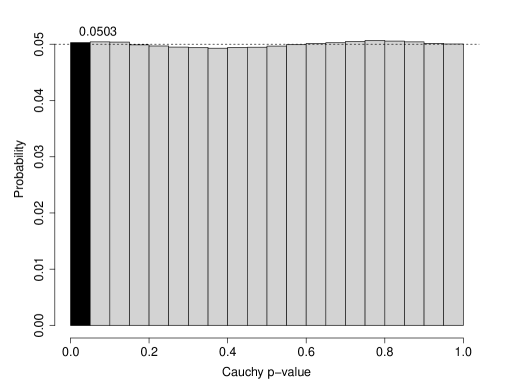
(a)

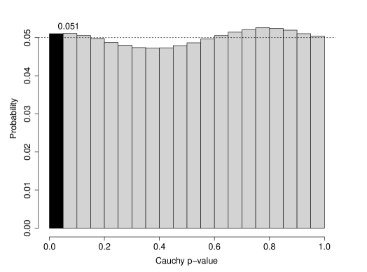
(b)

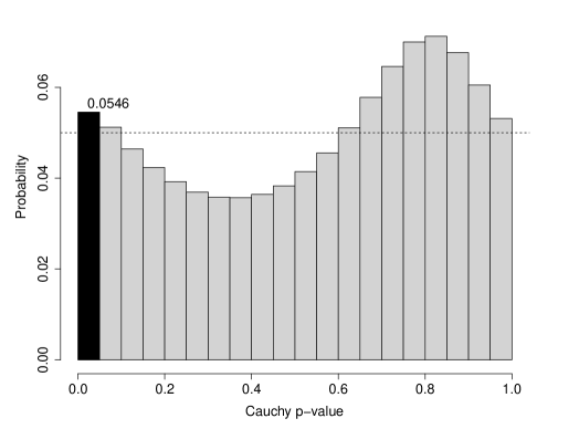
(c)

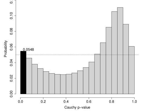
(d)

• Note: We plot histograms of GCC $p$-values (2.3) for various correlation strengths. The individual test statistics are drawn from a $d$-variate normal distribution $N_{d}(\bm{0},\bm{\Sigma})$ with $\bm{\Sigma}=(\sigma_{ij})$ and $d=300$. The diagonal elements of the covariance matrix $\sigma_{ii}=1$ for all $i=1,\ldots,d$ and the off-diagonal elements $\sigma_{ij}=\theta^{|i-j|}$ for $i\neq j$, with $\theta=0.2,0.4,0.8,0.95$. The simulation is repeated $10^{7}$ times. The simulated GCC $p$-values are sorted into bins with a width of 0.05. We highlight the first bin in black and add a text note with the probability of $p$-values being in the first bin.

2.3 Sequential Cauchy Combination Test

The main contribution of this paper is the introduction of the sequential Cauchy combination test, which extends the GCC test of Liu and Xie (2020) to make statements on the elementary hypotheses. To facilitate this, the raw $p$-values are sorted in ascending order, denoting them as $p_{(1)}\leq p_{(2)}\leq\ldots\leq p_{(d)}$, where $H_{(1)},H_{(2)},\ldots,H_{(d)}$ correspond to their respective null hypotheses. For the purpose of testing hypothesis $H_{\left(i\right)}$, we calculate a Cauchy combination test statistic, denoted as ${\normalsize\tilde{T}}_{\left(i\right)}$, using a subset of $p$-values running from $p_{(i)}$ to $p_{(d)}$ as:

$${\normalsize\ \tilde{T}_{\left(i\right)}=\sum_{j=i}^{d}w_{j}\tan\{(0.5-p_{(j)})\pi\}}\text{ \ with \ }w_{j}=\frac{1}{d-i+1},$$ (2.5)

where $w_{j}$ represents the weight assigned to each $p$-value in the subset. The corresponding $p$-value is computed as:

$$\widetilde{p}_{(i)}=\frac{1}{2}-\frac{\arctan\tilde{T}_{\left(i\right)}}{\pi}.$$ (2.6)

We reject the $i$th null hypothesis $H_{(i)}$ if $\widetilde{p}_{(i)}\leq\alpha$. Similar to the step-up procedure introduced by Hommel (1988), the SCC test leverages power across hypotheses: the test statistic $\tilde{T}_{(i)}$ is computed using the raw $p$-values associated with $\mathcal{H}_{0}^{(i)}=\bigcap_{j=i}^{d}H_{(j)}$.

A more prescriptive description of the SCC testing procedure is as follows:

Figure 2 illustrates the mechanics of sequential Cauchy combination procedure using a simulated sequence of test statistics. The top row of the figure shows the raw and ordered $p$-values. Most of the observations correspond to the null hypothesis (represented by grey dots), while a few observations correspond to the alternative hypothesis (represented by black dots). The data-generating process is the same as the one used in Figure 1, where $\theta=0.9$ and $d=100$. We add constant signals (nonzero mean) for five out of the 100 hypotheses, with a signal strength of $\pm 2.806$. The sign of the signal aligns with the sign of the test statistic under the null, such that the signal always amplifies the magnitude of the test statistic. The bottom row of the figure plots the sequential Cauchy combination test statistics (2.5) and their corresponding $p$-values (2.6). In particular, the bottom right panel shows that the SCC $p$-values $\widetilde{p}_{(i)}$ decrease as $i$ decreases from $d$ to $1$. In this example, the SCC test rejects three out of the five alternative hypotheses and does not reject any under the null hypothesis. These rejections correspond to the 4${}^{\text{th}}$, 29${}^{\text{th}}$ and 46${}^{\text{th}}$ hypotheses in the top left panel. It is worth noting that the smallest SCC $p$-value corresponds to the $p$-value of the GCC test in (2.1), which performs the test on the largest set of hypotheses.

Figure 2: Mechanics of the sequential Cauchy Combination test

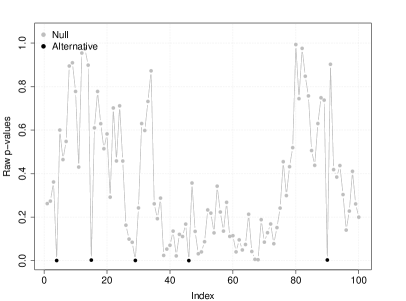
(a)

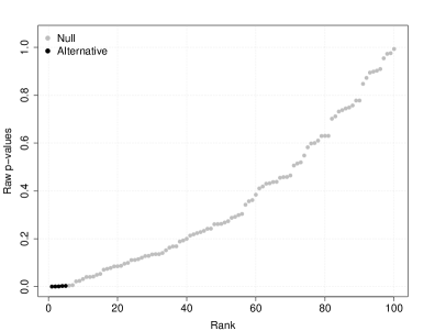
(b)

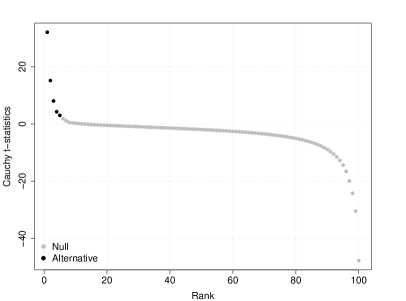
(c)

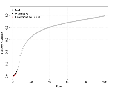
(d)

• Note: The test statistics are simulated from $N_{d}(\bm{0},\bm{\Sigma})$ as in Figure 1, with $d=100$, $\theta=0.9$ and $5\%$ signals. The strength of the signal is $\pm 2.806$, with its sign identical to that of the test statistic under the null. The horizon line in panel (d) is the 5% significance level.

The sequential Cauchy combination testing procedure requires two assumptions. Let $\bm{X}=(X_{1},X_{2},\ldots,X_{d})^{{}^{\prime}}$ represent the vector of test statistics.

Assumption 2.1

(1) The original test statistics $(X_{i},X_{j})$, for any $1\leq i<j\leq d$, follow a bivariate normal distribution; (2) $E\left(\bm{X}\right)=0$.

The requirement of bivariate normality in Assumption 2.1 is a condition weaker than joint normality, enabling the procedure to be applicable for high-dimensional settings. When the dimension $d$ increases at a certain rate with the sample size, the test statistics $\bm{X}$ may not jointly converge to a multivariate normal distribution due to a slower rate of convergence (see Liu and Xie, 2020, and references therein), and assuming joint normality becomes unrealistic in such settings.

Liu and Xie (2020) show through simulations that the global Cauchy approximation remains accurate even when the normality assumption is violated, and follows a multivariate Student-$t$ distribution (with four degrees-of-freedom) instead. For a showcase example in finance where the test statistics are Student-$t$ distributed, we refer the reader to Section 5.

Assumption 2.2

Let $\mathbf{\Sigma}=corr\left(\bm{X}\right)$. (1) The largest eigenvalue of the correlation matrix $\lambda_{\max}\left(\mathbf{\Sigma}\right)\leq C_{0}$ for some constant $C_{0}>0$; (2) $\max_{1\leq i<j\leq d}\left\{\sigma_{i,j}^{2}\right\}\leq\sigma_{\max}^{2}<1$ for some constant $0<\sigma_{\max}^{2}<1$, where $\sigma_{i,j}$ is the $\left(i,j\right)$ element of $\mathbf{\Sigma}$.

Assumption 2.2 on the correlation matrix becomes relevant when the number of hypotheses $d$ diverges to infinity. It imposes two conditions: boundedness of the largest eigenvalue of the correlation matrix and the absence of perfectly correlated test statistics. The conditions are frequently encountered in high-dimensional settings and general enough to encompass a wide range of tests.

Theorem 1

Under Assumption 2.1 for a fixed $d$ and Assumptions 2.1 and 2.2 for $d=o(h^{\eta})$ with $0<\eta<1/2$, as $\alpha\rightarrow 0$, the probability of the SCC testing procedure making at least one false rejection converges to $\alpha$, i.e.,

$$\lim_{\alpha\rightarrow 0}\Pr\left\{\mathcal{R}\cap\mathcal{T}=\emptyset\right\}\rightarrow\alpha.$$ (2.7)

The proof of Theorem 1 is provided in Appendix A. The theoretical result in (2.7) for the SCC testing procedure stands in stark contrast to statistical inequality-based controlling procedures covered in the Online Supplement, which have the property:

$$\Pr\left\{\mathcal{R}\cap\mathcal{T\neq\emptyset}\right\}\leq\alpha.$$

See Goeman and Solari (2010) for a discussion of their theoretical properties. These inequality-based controlling procedures ensure that the likelihood of making at least one false discovery is bounded above by the pre-specified significance level, $\alpha$. Consequently, the SCC procedure exhibits less conservatism compared to inequality-based controlling procedures.

3 Simulations

In this section, we compare the performance of the SCC test against several popular multiple testing corrections in a simulation study, considering different forms of dependence. The benchmark procedures include four inequality-based approaches: the Bonferroni correction and its subsequent improvements proposed by Holm, 1979, Hommel, 1988 and Hochberg, 1988, as well as the Gumbel approach. Detailed discussions of these benchmark procedures can be found in the Online Supplement.

3.1 Under the null hypothesis

We assess the statistical performance of the different multiple testing corrections under the null hypothesis. To measure the empirical familywise error rate, we conduct $S=10^{4}$ replications for each method $m$, and calculate $\widehat{FWER}_{m}$ as follows:

$$\widehat{FWER}_{m}=\frac{1}{S}\sum_{s=1}^{S}\bm{1}\left(\min_{i\in\left\{1,2,\cdots,d\right\}}\left\{p_{(m,i)}^{s}\right\}\leq\alpha\right),$$

where $\bm{1}(.)$ is the indicator function, and $p_{(m,i)}^{(s)}$ represents the $p$-value of the $i$th hypothesis for method $m$ in the $s$th replication. When the test statistics exhibit strong dependence, we expect the $\widehat{FWER}$ of the SCC test to be closer to the nominal level $\alpha$ compared to the other procedures.

Under the null hypothesis, the test statistics $\bm{X}$ are generated from a $d$-variate normal distribution with zero mean and covariance matrix $\bm{\Sigma}$, i.e., $N_{d}(\bm{0},\bm{\Sigma})$. We set the dimension $d$ to 100. The diagonal elements of the covariance matrix, $\sigma_{ii}$, are all equal to $1$, for $i=1,\ldots,d$. The off-diagonal element, $\sigma_{ij}$ with $i\neq j$, adhere to three specific specifications.

• Model 1. Exponential decay: $\sigma_{ij}=\theta^{\absolutevalue{i-j}}$ with $\theta=0.2,0.4,0.6,$ $0.8,0.90,0.95$.

• Model 2. Polynomial decay: $\sigma_{ij}=\frac{1}{0.7+\absolutevalue{i-j}^{\theta}}$ with $\theta=1.0,1.5,2.0,2.5$.

• Model 3. Block-diagonal: $\bm{\Sigma}=\text{diag}\{A_{1},\ldots,A_{d/10}\}$, for which each diagonal block $A_{k}$ is a $10\times 10$ equi-correlation matrix with its off-diagonals $\sigma_{ij}=\theta$ and $\theta=0.1,0.3,0.5,0.7,0.9$.

Models 1 and 2 also appear in Liu and Xie (2020). The exponentially decaying correlation structures in Model 1 are frequently observed in time series and financial econometrics. For instance, in Section 4.1, the sequence of drift burst test statistics constructed from overlapping rolling windows, exhibits an autoregressive process and has an exponential decaying covariance structure, as shown by Christensen et al. (2022). The block-diagonal structure in Model 3 is commonly used when testing high-dimensional factor pricing models (see e.g., the Monte Carlo experiments in Fan et al., 2015) and emulates a cross-sectional dependence structure.

Table 1 shows the superior performance of the SCC test in the presence of correlated test statistics under the null hypothesis. The empirical familywise error rate of the SCC test, reported in the last column, remains close to the nominal level $\alpha=5\%$ across various correlation structures, demonstrating its robustness. These findings align with the theoretical discussions presented in Section 2. In contrast, the inequality-based procedures and the Gumbel method exhibit greater conservatism, as evidenced by their substantially lower FWERs (although slight variations exist depending on the correlation pattern). The SCC test stands out as the only controlling procedure with an empirical FWER close to the nominal level (5%) across all three types of correlation structures in the test statistics.

Table 1: Empirical FWERs (in%) of the controling procedures

$\theta$ Bonferroni Holm Hommel Hochberg Gumbel SCC Model 1: Exponential decay 0.2 4.68 4.68 4.68 4.68 $\underline{3.30}$ 4.94 0.4 4.88 4.88 4.88 4.88 $\underline{3.44}$ 5.36 0.6 4.96 4.96 4.96 4.96 $\underline{3.54}$ 5.78 0.8 $\underline{3.98}$ $\underline{3.98}$ $\underline{4.00}$ $\underline{3.98}$ $\underline{2.84}$ 5.82 0.9 $\underline{2.40}$ $\underline{2.40}$ $\underline{2.42}$ $\underline{2.40}$ $\underline{1.70}$ 5.48 0.95 $\underline{1.76}$ $\underline{1.76}$ $\underline{1.78}$ $\underline{1.76}$ $\underline{1.18}$ 5.38 Model 2: Polynomial decay 1.0 4.70 4.70 4.70 4.70 $\underline{3.38}$ 5.96 1.5 4.62 4.62 4.62 4.62 $\underline{3.62}$ 5.48 2.0 4.44 4.44 4.44 4.44 $\underline{3.18}$ 5.38 2.5 4.46 4.46 4.46 4.46 $\underline{3.16}$ 5.14 Model 3: Block-diagonal 0.1 4.56 4.56 4.58 4.56 $\underline{3.50}$ 4.92 0.3 4.74 4.74 4.76 4.74 $\underline{3.74}$ 5.32 0.5 4.54 4.54 4.54 4.54 $\underline{3.28}$ 5.70 0.7 $\underline{3.40}$ $\underline{3.40}$ $\underline{3.40}$ $\underline{3.40}$ $\underline{2.46}$ 5.62 0.9 $\underline{1.88}$ $\underline{1.88}$ $\underline{1.92}$ $\underline{1.88}$ $\underline{1.30}$ 5.62 Note: We report the empirical FWERs (frequencies of falsely rejecting at least one hypothesis) of the controlling procedures. The test statistics are generated from $N_{d}(\bm{0},\bm{\Sigma})$ with different correlation structures. The dimension $d$ is $100$ and the nominal significance level $\alpha$ is 5%. The number of replications is $10^{4}$. Instances with lower than 4% FWER are underlined.

3.2 Under the alternative hypothesis

Under the alternative hypothesis, the performance of the controlling procedures is assessed based on their global power (the percentage of replications that reject at least one hypothesis) and their successful detection rate (the percentage of overlapping hypotheses between the sets of false hypotheses and discoveries). Given the improved accuracy of the SCC procedure in controlling the FWER under the null hypothesis (as demonstrated in Table 1), we anticipate that the SCC test will exhibit higher power when applied under the alternative hypothesis.

The test statistic vector $\bm{X}$ is generated from a $d$-variate normal distribution with mean vector $\bm{\mu}=(\mu_{i})$ and a correlation matrix $\bm{\Sigma}=(\sigma_{ij})$, i.e., $N_{d}(\bm{\mu},\bm{\Sigma})$. We adopt the same correlation matrices $\bm{\Sigma}$ as discussed in Section 3.1. The percentage of signals (i.e., non-zero $\mu_{i}$’s in the vector $\bm{\mu}$) is set to be 5% (specifically, out of the 100 hypotheses, 5 are under the alternative). All signals have the same strength $\absolutevalue{\mu_{i}}=\mu_{0}$ which is chosen to be relatively weak, i.e., $\pm 2.1737$. The sign of the signal aligns with the sign of the test statistic under the null so that the signal always amplifies the magnitude of the test statistic.

Table 2: Global power (in%) in a correlated setting with sparse signals

$\theta$ Bonferroni Holm Hommel Hochberg Gumbel SCC Model 1: Exponential decay 0.2 66.50 66.50 66.62 66.50 $\underline{59.32}$ 76.20 0.4 66.48 66.48 66.60 66.48 $\underline{59.86}$ 76.84 0.6 65.70 65.70 65.74 65.70 $\underline{58.58}$ 75.82 0.8 $\underline{63.86}$ $\underline{63.86}$ $\underline{63.90}$ $\underline{63.86}$ $\underline{56.90}$ 72.74 0.9 $\underline{60.62}$ $\underline{60.62}$ $\underline{60.78}$ $\underline{60.64}$ $\underline{53.90}$ 68.42 0.95 $\underline{57.24}$ $\underline{57.24}$ $\underline{57.30}$ $\underline{57.24}$ $\underline{50.58}$ 63.94 Model 2: Polynomial decay 1.0 66.04 66.04 66.14 66.04 $\underline{58.76}$ 74.82 1.5 65.88 65.88 66.00 65.88 $\underline{58.46}$ 75.10 2.0 65.88 65.88 66.00 65.88 $\underline{58.84}$ 75.20 2.5 65.22 65.22 65.28 65.22 $\underline{58.22}$ 74.66 Model 3: Block-diagonal 0.1 66.44 66.44 66.50 66.44 $\underline{59.84}$ 76.50 0.3 67.10 67.10 67.18 67.10 $\underline{60.40}$ 76.00 0.5 65.84 65.84 65.94 65.84 $\underline{58.48}$ 74.44 0.7 $\underline{63.72}$ $\underline{63.72}$ $\underline{63.74}$ $\underline{63.72}$ $\underline{57.34}$ 71.62 0.9 $\underline{60.88}$ $\underline{60.88}$ $\underline{61.02}$ $\underline{60.88}$ $\underline{54.10}$ 69.22 Note: We report the global powers (frequencies of rejecting at least one hypothesis), for various correlation matrices in the presence of sparse signals. The test statistics are generated from $N_{d}(\bm{\mu},\bm{\Sigma})$ with different correlation structures and sparse signals. The dimension $d$ is fixed at $100$, and the percentage of signals is set to $5\%$. All the signals have the same strength ($\pm 2.1737$), with the sign depending on the sign of the test statistic under the null. We use a nominal significance level of 5% and conduct $10^{4}$ replications. We underline instances where the FWERs were lower than 4% in Table 1.

Table 2 shows the superior global power of the SCC test in the presence of correlated test statistics and sparse signals. The SCC test exhibits an approximate $10$% power enhancement compared to the runner-up method. When the significance level $\alpha$ is set to $5\%$, the power of the SCC test ranges between $69$% and $77$%. Although each statistical inequality-based method improves upon its predecessor in certain aspects, we do not observe a significant difference in the frequency of rejections among the four approaches. As anticipated, the Gumbel approach, which assumes independent test statistics, is the most conservative test.

Table 3 tells a similar story with respect to the average numbers of successful detections. The SCC testing procedure successfully detects approximately 1.2 out of 5 hypotheses (or $24\%$) under the alternative, even with sparse and weak signals. Meanwhile, the average number of successful detection for the inequality-based procedures are around 0.95 (or $19\%$), whereas the value for the Gumbel procedure is about 0.81 (or $16.2\%$).

Table 3: Successful detection rates (in%) in a correlated setting with sparse signals

$\theta$ Bonferroni Holm Hommel Hochberg Gumbel SCC Model 1: Exponential decay 0.2 18.80 19.00 19.00 19.00 $\underline{16.00}$ 23.20 0.4 19.20 19.20 19.20 19.20 $\underline{16.20}$ 23.60 0.6 18.80 19.00 19.00 19.00 $\underline{16.00}$ 23.40 0.8 $\underline{19.20}$ $\underline{19.40}$ $\underline{19.40}$ $\underline{19.40}$ $\underline{16.20}$ 24.00 0.9 $\underline{19.00}$ $\underline{19.00}$ $\underline{19.20}$ $\underline{19.00}$ $\underline{16.00}$ 24.00 0.95 $\underline{19.20}$ $\underline{19.20}$ $\underline{19.20}$ $\underline{19.20}$ $\underline{16.20}$ 24.40 Model 2: Polynomial decay 1.0 19.00 19.20 19.20 19.20 $\underline{16.00}$ 23.60 1.5 19.00 19.20 19.20 19.20 $\underline{16.00}$ 23.40 2.0 19.00 19.20 19.20 19.20 $\underline{16.00}$ 23.60 2.5 18.80 18.80 18.80 18.80 $\underline{16.00}$ 23.40 Model 3: Block-diagonal 0.1 19.40 19.40 19.40 19.40 $\underline{16.40}$ 23.60 0.3 19.40 19.60 19.60 19.60 $\underline{16.60}$ 23.60 0.5 19.40 19.40 19.40 19.40 $\underline{16.40}$ 23.80 0.7 $\underline{19.20}$ $\underline{19.40}$ $\underline{19.40}$ $\underline{19.40}$ $\underline{16.40}$ 23.80 0.9 $\underline{19.00}$ $\underline{19.00}$ $\underline{19.00}$ $\underline{19.00}$ $\underline{16.20}$ 23.80 Note: We report the successful detection rates (overlap between the sets of alternative hypotheses and discoveries). The data-generating processes used are the same as those for Table 2. We use a nominal significance level of 5% and conduct $10^{4}$ replications. We underline instances where the FWERs were lower than 4% in Table 1.

4 Example 1: Monitoring Drift Burst

The drift burst hypothesis, as proposed by Christensen et al. (2022), postulates the existence of locally explosive trends in high-frequency asset prices, resembling phenomena like flash crashes or gradual jumps. An infamous example of a flash crash occurred on May 6, 2010, when the Dow Jones Industrial Average rapidly dropped nearly 1,000 points within minutes, only to recover most of the losses shortly thereafter.

The drift burst test serves to detect and timestamp these explosive trends. In our analysis, we compute the test statistic on a minute-by-minute basis. Since there are 6.5 trading hours per day, the test needs to be conducted 341 times per day, resulting in a multiple testing problem. The test statistics are computed using overlapping windows and are expected to exhibit high autocorrelation. Given that drift bursts are rare events, they can be considered as sparse signals, and the strength of these signals can vary. There are several approaches to deal with the false discovery problem in this context, including the benchmark procedures considered in Section 3, the SCC, test and a resampling procedure suggested by Christensen et al. (2022).

Section 4.1 presents the drift burst hypothesis and the drift burst test as a means to detect these phenomena. In Section S2.3 of the Online Supplement, we conduct a simulation study. We apply the controlling procedures to detect drift bursts in real-world data, specifically the Nasdaq composite index and S&P 500 index ETFs, in Section 4.2.

4.1 Drift Burst Hypothesis and Test

Under the null hypothesis of no drift burst, the frictionless log prices $P=(P_{t})_{t\geq 0}$ follow an Itô semi-martingale process defined on a filtered probability space $(\Omega,\mathcal{F},(\mathcal{F})_{t\geq 0},\mathbb{P})$:

$$dP_{t}=\mu_{t}dt+\sigma_{t}dW_{t},$$ (4.1)

where $\mu_{t}$ is the instantaneous drift, and the diffusive component consists of the spot volatility $\sigma_{t}$ and a standard Brownian motion $W_{t}$. The coefficients $\mu_{t}$ and $\sigma_{t}$ are locally bounded or “non-explosive”. The volatility process is assumed to follow a Heston (1993)-type dynamics:

$$d\sigma_{t}^{2}=\kappa\left(\omega-\sigma_{t}^{2}\right)dt+\xi\sigma_{t}dB_{t},$$

where $B_{t}$ is a standard Brownian motion and $E\left(dW_{t},dB_{t}\right)=rdt$.

Under the alternative hypothesis, a drift-bursting term $\mu_{t}^{\text{b}}$ and a volatility-bursting component $\sigma_{t}^{\text{b}}$ are added to the standard Itô semi-martingale process (4.1), resulting in the following dynamics:

$$d{P}_{t}= \mu_{t}dt+\sigma_{t}dW_{t}+\mu_{t}^{\text{b }}dt+\sigma_{t}^{\text{b}}dW_{t},$$ (4.2)

where $\absolutevalue{\mu_{t}^{\text{b}}}/\sigma_{t}^{\text{b}}\rightarrow\infty$ as $t\rightarrow\tau_{\text{b}}$, with $\tau_{\text{b}}$ denoting the drift burst time. An example of such an explosive process is given by:

$$\mu_{t}^{\text{b}}=a\frac{\text{sign}(t-\tau_{\text{b}})}{\absolutevalue{\tau_{\text{b}}-t}^{\alpha^{\text{b}}}}\,\,\text{and}\,\,\sigma_{t}^{\text{b}}=b\frac{\sqrt{\omega}}{\absolutevalue{\tau_{\text{b}}-t}^{\beta^{\text{b}}}},\,\,\text{for}\,\,t\in[\tau_{\text{b}}-\Delta t,\tau_{\text{b}}+\Delta t],$$ (4.3)

where $2\Delta t$ represents the duration of the burst, $\alpha^{\text{b}}$ corresponds to the strength of the burst, $\beta^{\text{b}}$ is the strength of the volatility burst and $a$ and $b$ are constants. This data-generating process can capture various realistic patterns, including flash crashes and mildly explosive trends, and is used in the simulations in Section S2.3.

Observations are recorded at equidistant intervals $0=t_{0}<t_{1}<\ldots<t_{n}=T$, where $T$ represents a fixed time period, such as one trading day consisting of 6.5 trading hours. The distance between two consecutive observations is $\Delta_{n}=t_{i+1}-t_{i}$. The observed log price, contaminated by noise, is denoted as $\widetilde{P}_{t_{i}}=P_{t_{i}}+\epsilon_{t_{i}}$, where the $\epsilon$ is an error term (noise) and independent from the latent log price $P$.

The noise-robust drift burst statistic (Christensen et al., 2022) is defined as:

$$X_{i}=\sqrt{h}\frac{\hat{\bar{\mu}}_{t_{i}}}{\sqrt{\hat{\bar{\sigma}}_{t_{i}}^{2}}},$$ (4.4)

where $h$ is the bandwidth of the mean estimator, $\hat{\bar{\mu}}_{t_{i}}$ is a noise-robust estimator for the local drift, and $\hat{\bar{\sigma}}_{t_{i}}^{2}$ is a noise-robust estimator for the local variance. The test is applied on a coarse sampling grid, and the null hypothesis of the drift burst test asserts that ‘there is no drift bursting at time period $t_{i}$’. The drift burst test statistics are computed minute-by-minute using overlapping rolling windows. As a result, the dimension of the test statistic sequence $\bm{X}=\left\{X_{i}\right\}$ is large (with the parameters settings we end up with $d=341$ for the period of one day) and the tests are autocorrelated. For more information regarding the implementation of noise-robust estimators of the local drift and local variance, we refer the reader to the Online Supplement.

Under the null hypothesis, as the sampling frequency approaches infinity ($\Delta_{n}\rightarrow 0$), the test statistic (4.4) converges to the standard normal distribution, i.e., $X_{i}\rightarrow^{d}N(0,1)$, This implies that the test statistic satisfies the necessary assumptions required by the Cauchy combination test when the sampling frequency is sufficiently high under the null. Under the alternative hypothesis, the test statistic diverges when the drift term explodes fast enough relative to the volatility, i.e., $\absolutevalue{X_{i}}\rightarrow\infty$, at the drift burst time.

To control the familywise error rate, Christensen et al. (2022, Appendix B) propose a resampling-based approach for generating critical values for the drift burst test. The resampling approach approximates the dependence structure of the test statistic sequence under the null hypothesis with an autoregressive order one (i.e., AR(1)) model and to obtain its distribution via simulation.

There are a few limitations associated with using simulated critical values in practice. Since each sequence of test statistics (corresponding to each day in an empirical analysis or each sample path in a Monte Carlo study) requires a unique critical value, the resampling procedure is computationally intensive. It also imposes a strong parametric assumption on the dependence structure, which could be misspecified. Additionally, resampling attempts to reproduce the dependence structure under the null hypothesis using possibly contaminated data (as seen in the attenuation bias reported in Christensen et al., 2022), which in turn can affect the estimation of the critical value. Therefore, caution should be exercised when interpreting the results, and the potential biases associated with the parameter estimation must be considered. See the Online Supplement for more detailed discussion of the resampling approach.

In the Online Supplement, we also evaluate the performance of the aforementioned controlling procedures in a simulation setting. Specifically, we evaluate the performance of the four inequality-based procedures, the Gumbel method, the resampling approach, and the SCC testing procedure. Instead of directly simulating the test statistics as done in Section 3, we generate log prices from (4.1) under the null hypothesis and (4.3) under the alternative hypothesis, and then compute drift burst test statistics (4.4) from the simulated prices. Two types of drifts bursts are considered: a V-shaped 20-minute flash crash and a three-day persistent expansion.

Our findings suggest that the SCC procedure is the most preferred option for monitoring drift bursts. The inequality-based methods and the Gumbel method tend to be conservative when applied to the autocorrelated drift burst test statistics. While the resampling procedure shows slightly better performance in terms of power and successful detection rate for flash crashes, the SCC procedure significantly outperforms the resampling method in identifying persistent expansions. Although there might be a small loss in power observed in some specific cases, it is a reasonable trade-off for having a robust approach to monitor drift bursts. Moreover, the SCC procedure procedure offers the advantage of being easier to implement and can accommodate arbitrary dependency structures without requiring simulations, making it a more practical choice overall.

4.2 Empirics

We apply the same controlling procedures to the drift burst test using data from the Nasdaq ETF (ticker: IXIC) and the S&P 500 ETF (ticker: SPY) covering the period from 1996 to 2020. The data was obtained from the Refinitiv Tick History Database at a one-second frequency, and we follow the data cleaning rules outlined in Barndorff-Nielsen et al. (2009). We test for drift bursts on a minute-by-minute basis and control the familywise error rate at a level of $0.1$%.

The weekly prices of the Nasdaq and S&P 500 ETFs are illustrated in Figure 3, with grey bars indicating weeks that exhibit drift bursts. Drift bursts are determined using the test proposed by Christensen et al. (2022) and the SCC controlling procedure. It is evident that the Nasdaq index experienced a higher number of drift bursts, particularly in the early 2000s following the collapse of the dot-com bubble. The S&P 500 index barely has any rejections.

Figure 3: Drift bursts in the Nasdaq and S&P 500 ETFs from 1996 to 2020

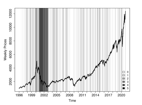
(a)

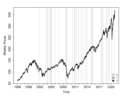
(b)

• Note: The black lines are the weekly index ETF prices. The grey bars indicate the number of rejections of the ‘no drift burst’ null within the week. The darker the grey scale the more drift burst days we observe. We use the drift burst test of Christensen et al. (2022) and the SCC testing procedure to control for the FWER at the $0.1\%$ significance level.

Table 4 reports the rejection frequencies of the drift burst test using the aforementioned controlling procedures. Compared to the benchmark procedures, the SCC test demonstrates a higher sensitivity in detecting drift burst days (i.e., at least one rejection within the day) and time intervals (i.e., the total number of rejections) in the Nasdaq index. In the case of the S&P 500 index ETF, the SCC testing procedure detects more drift burst days and intervals than the inequality-based and Gumbel methods, albeit slightly fewer than the resampling procedure. It is noteworthy that the bursting episodes in the S&P 500 are relatively short-lived, aligning with the Flash Crash data-generating process considered in our simulations. On the other hand, the Nasdaq index exhibits persistent drifts (as reported in Laurent and Shi, 2022), akin to the persistent expansion data-generating process.

Table 4: Rejection frequencies of the drift burst test: Nasdaq and S&P 500 index ETFs

	Bonferroni	Holm	Hommel	Hochberg	Gumbel	Resampling	SCC
Nasdaq
Days (in%)	18.840	18.840	18.840	18.840	11.662	23.357	23.522
Intervals (in#)	6,479	6,540	6,559	6,540	3,823	8,633	10,944
S&P 500
Days (in%)	0.526	0.526	0.526	0.526	0.247	0.641	0.576
Intervals (in#)	41	41	41	41	18	55	50

• Note: The drift burst days are percentages of days over the full sample period with at least one rejection. The figures in rows labelled intervals (in#) are the total number of rejections over the entire sample period.

5 Example 2: In Search of Nonzero Alpha Assets

The Capital Asset Pricing Model (CAPM) is a prominent risk model. However, in light of empirical evidence revealing systematic patterns in stock returns, often referred to as “anomalies”, many additional risk factors have been introduced to explain average returns. These risk factors are said to represent some dimension of undiversifiable systematic risk that should be compensated with higher returns. If the factor model fully characterizes expected returns, the regression intercept (also known as the “alpha”) should theoretically equal zero.

We search for nonzero alpha assets using the Fama and French (2015) five-factor model framework. The conventional approach is to run time series regressions on each individual asset, and subsequently perform individual tests on the estimated alphas. The number of assets that need to be tested simultaneously is large (e.g., all of the S&P 500 stocks) and the test statistics of the cross-sectional alphas are most likely correlated due to the presence of unknown common factors (see e.g., Giglio et al., 2021). There is a general consensus in the empirical finance literature that mispriced assets are rare (see e.g., Fan et al., 2015; Giglio et al., 2021). To tackle the challenge of multiple testing, several methods can be used. These include the benchmark procedures, the SCC test, and a screening procedure proposed by Fan et al. (2015). All of these procedures control the FWER and have the ability to identify individual violations.

Section 5.1 provides an overview of the nonzero alpha hypothesis and introduces the corresponding test. Section S3.2 of the Online Supplement presents simulation results that compare the performance of the controlling procedures in the context of the nonzero alpha test. In Section 5.2, we examine Fama-French portfolios formed on bivariate sorts and search for portfolios with a nonzero alpha.

5.1 Nonzero Alpha Hypothesis and Test

The multi-factor pricing model, motivated by the Arbitrage Pricing Theory (Ross, 1976), postulates how financial returns are related to market risks. This model has enjoyed widespread application in asset pricing and portfolio management. Let $y_{it}$ be the excess return (i.e., real rate of return minus the risk-free rate) of the $i$th financial asset at day $t$ and consider the following linear regression model:

$$y_{it}=a_{i}+\bm{b}^{\prime}_{i}\bm{f}_{t}+u_{it},\quad\text{with }i=1,\ldots,d,\,t=1,\ldots,T,$$ (5.1)

where $a_{i}$ is an intercept, often referred to as “alpha”, $\bm{b}_{i}=(b_{i1},\ldots,b_{iK})^{\prime}$ is a vector of factor sensitivities or loadings, also known as “betas”, $\bm{f}_{t}=(f_{1t},\ldots,f_{Kt})^{\prime}$ are observable factors, and $u_{it}$ is an idiosyncratic error which is uncorrelated with the factors. A well-known example of (5.1) is the three-factor model of Fama and French (1992), which captures a substantial portion of the variation in the cross-section of average returns and absorbs a lot of the anomalies that have plagued the CAPM (see also Fama and French, 1996).

Our objective is to identify individual assets with a nonzero alpha. The null hypothesis of each asset is therefore $H_{i}:a_{i}=0$ (‘there is no mispricing of asset $i$’) and the alternative hypothesis is $a_{i}\neq 0$ (‘asset $i$ is mispriced’), for $i=1,\ldots,d$. The most common way to test this null hypothesis is to use a simple $t$-statistic for $a_{i}$, i.e.,

$${X}_{i}=\frac{\hat{a}_{i}}{\hat{\sigma}_{\hat{a}_{i}}},$$ (5.2)

where $\hat{a}_{i}$ is the estimated alpha and $\hat{\sigma}_{\hat{a}_{i}}$ is the estimated standard error, for each asset $i=1,...,d$. Under the null hypothesis, the test statistic (5.2) follows a Student-$t$ distribution, i.e., $X_{i}\sim t(\nu)$, with $\nu$ being the degrees of freedom. A viable detection strategy involves computing the test statistic (5.2) for each asset in the cross-section and rejecting the null hypothesis when $\absolutevalue{X_{i}}$ exceeds a pre-specified quantile of the $t(\nu)$ distribution.

The multiplicity issue arises when dealing with a large number of assets. One important benchmark for controlling false discoveries in testing factor pricing models is the power enhancement test proposed by Fan et al. (2015). This global test employs a screening technique that incidentally identifies individual violations. We refer to this approach as the screening method and provide a comprehensive description of the procedure in the Online Supplement. We can also use other approaches such as the inequality-based, Gumbel method and SCC test. It is worth noting that the cross-sectional test statistics are likely to be cross-correlated (see e.g., Giglio et al., 2021), and hence the Gumbel method and inequality-based procedures are again expected to be conservative. While it is true that a Student-$t$ distribution does not exactly fulfill the assumptions of the Cauchy combination test, Liu and Xie (2020) show through simulations that the Cauchy approximation remains accurate under such a departure from normality.

Once again, we assess the finite sample performance of the SCC testing procedure by comparing it with existing controlling procedures, which include the four inequality-based procedures, the Gumbel method and the screening approach, for the identification of nonzero alpha assets in both simulation settings and empirical applications. We exclude the resampling approach considered for the drift burst test, as it is not suitable for the current cross-sectional context. Complete details of the simulation designs and results can be found in the Online Supplement. Unlike the simulations in Section 3, we simulate excess returns from the Fama and French (2015) five-factor model, with its parameters calibrated to the empirical data. We then compute the test statistics from the simulated data. Our findings show that the SCC test outperforms all other procedures in terms of controlling the FWER, global power, and successful detection rate. The Gumbel method and screening method tend to be most conservative in their outcomes.

5.2 Empirics: Kenneth French Portfolios

In the empirical analysis, we study the portfolios available in Kenneth French’s Data Library. Specifically, we focus on the $d=100$ portfolios formed bivariately ($10\times 10$) based on size and book-to-market (Size-BM), size and investment (Size-INV), and size and operating profitability (Size-OP). The left-hand side of equation (5.1) comprises value-weighted portfolio excess returns and the right-hand side are the five factors in the Fama and French (2015) five-factor model (i.e., market, value, size, profitability and investment). The sample period spans from July 1963 to November 2022 and consists of $713$ monthly observations. To conduct the nonzero alpha test, we use a rolling window approach with a window size of $T=240$ observations. We treat the $100$ portfolios as one family and control the familywise error rate at the $5\%$ level.

Table 5 reports the average rejection frequencies of zero alpha null (across the rolling analysis) using various controlling procedures. As anticipated, there are few violations. For instance, in the case of the Size-BM portfolios, the SCC test shows an average rejection frequency of 2.60%. Overall, the SCC test consistently yields higher rejection frequencies compared to the inequality-based methods, the screening procedure, and the Gumbel method, in that order. These empirical results align with prior research on mispricing, confirming the rarity of nonzero alpha assets (see e.g., Fama and French, 1996; Fan et al., 2015; Giglio et al., 2021). Nonetheless, the SCC testing procedure can detect more of these rare violations.

Table 5: Average rejection frequencies (in%) of zero alpha null across a rolling analysis

Bonferroni Holm Hommel Hochberg Gumbel Screening SCC Size-BM 1.25 1.26 1.27 1.26 1.09 1.09 2.60 Size-OP 0.53 0.53 0.53 0.53 0.51 0.61 0.75 Size-INV 1.19 1.19 1.19 1.19 1.13 1.15 1.40

Note: We test the zero alpha null hypotheses within the Fama-French five-factor model framework using various controlling procedures. The nominal level is 5% and the rolling window size is $T=240$.

Evidently, the rejection numbers vary over time, as can be seen in Figure 4. In the first decade of the sample period, there is almost zero rejection according to all procedures. The number of identified nonzero portfolios starts to increase in the late 1990s, reaching its peak during the dot-com bubble crash in the early 2000s, and declined afterwards. The SCC test identifies more violations than other procedures for about $40\%$ of the sample period. During the remaining periods, the rejection numbers of the SCC test are on par with the other procedures. While the results from the benchmark procedures are similar, the gap between the SCC test and other procedures can be very substantial. For instance, in March 2001, the SCC test detected 13 portfolios with nonzero alphas, while the benchmark procedures identify only 1 or 2 such portfolios. The findings above align with our theoretical expectations and are consistent with our previous simulations results, reinforing the notion that using SCC can yield significant improvements in testing outcomes.

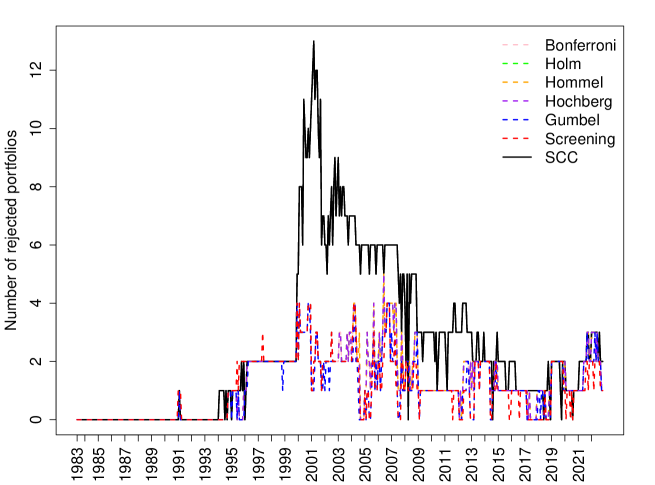
Figure 4: Number of rejected Size-BM portfolios from 1963 to 2022

• Note: The nominal level is 5% and the rolling window size is $T=240$.

6 Conclusions

We introduce a simple procedure to control for false discoveries and identify individual signals in scenarios involving many tests, dependent test statistics, and potentially sparse signals. The tool is agnostic to the underlying dependence structure and scalable to deal with high dimensions. Our approach is a sequential version of the global Cauchy combination test proposed by Liu and Xie (2020). By applying the global test recursively on a sequence of expanding subsets of ordered $p$-values, our sequential Cauchy combination test enables the identification of individual violations.

We show that the sequential Cauchy combination test achieves strong familywise error rate control and is less conservative compared to popular statistical inequality-based methods (such as the Bonferroni correction and subsequent improvements of Holm, 1979, Hommel, 1988 and Hochberg, 1988) and the Gumbel method.

The Cauchy transformation has proven its value in a genome-wide association study of Crohn’s disease (Liu and Xie, 2020, Section 4.3), but its applicability extends beyond genomics. We revisit two important needle-in-a-haystack problems in financial econometrics, where the test statistics have either serial or cross-sectional dependence: monitoring drift bursts and searching for nonzero alpha assets. The drift burst test of Christensen et al. (2022) detects the presence of explosive trends in asset prices using high-frequency intraday data. The test statistics are computed from overlapping windows, resulting in high autocorrelation. We also revisit the Fama and French (2015) multi-factor model to identify nonzero alpha financial assets. Detecting these rare nonzero alphas among a large group of financial assets is challenging, especially when the test statistics are likely to be cross-sectionally correlated. Without a proper controlling procedure, one might flag false discoveries or miss important signals. Our results indicate that the sequential Cauchy combination test is the a preferable method for both applications.

We emphasize that our sequential Cauchy combination test is not limited to financial econometrics. We anticipate its applicability to a wide range of hypothesis tests in fields such as economics, finance, medicine, marketing and climate studies, as it can handle various types of dependence effectively.

Appendix A Proof of Theorem 1

Proof. Let $\mathcal{R}^{(s)}$ be the collection of rejected hypotheses in step $s$ with $s=\left\{1,2,\ldots,d\right\}$, $\mathcal{R}^{(0)}=\emptyset$, and the rejection set $\mathcal{R}=\mathcal{R}^{(d)}$. The SCC testing procedure can be viewed as a sequential rejection procedure, as outlined in Table 6.

Table 6: Sequential rejection procedure of the SCC test

Step	Hypothesis	Decision
$s=1$	$\mathcal{H}_{0}^{\left(1\right)}=\bigcap_{j=1}^{d}H_{(j)}$	$\mathcal{R}^{(1)}=H_{(1)}$ if $\widetilde{p}_{(1)}\leq\alpha$; otherwise $\mathcal{R}^{(1)}=\emptyset$
$s=2$	$\mathcal{H}_{0}^{\left(2\right)}=\bigcap_{j=2}^{d}H_{(j)}$	$\mathcal{R}^{(2)}=\mathcal{R}^{(1)}\cup H_{(2)}$ if $\widetilde{p}_{(2)}\leq\alpha$; otherwise $\mathcal{R}^{(2)}=\mathcal{R}^{(1)}$
$\ldots$	$\ldots$	$\ldots$
$s=d$	$\mathcal{H}_{0}^{\left(d\right)}=H_{(d)}$	$\mathcal{R}^{(d)}=\mathcal{R}^{(d-1)}\cup H_{(d)}$ if $\widetilde{p}_{(d)}\leq\alpha$; otherwise $\mathcal{R}^{(d)}=\mathcal{R}^{(d-1)}$

Let $\mathcal{N}_{s}\left(\mathcal{R}^{(s-1)}\right)$ be the successor function, which represents hypotheses to be rejected at the step $s$ given $\mathcal{R}^{(s-1)}$. The successor function of the SCC test is defined by:

$$\mathcal{N}_{s}\left(\mathcal{R}^{(s-1)}\right)=\left\{\begin{array}[]{ll}H_{(s)}&\text{if }\widetilde{p}_{(s)}\leq\alpha_{\mathcal{R}^{(s-1)}}=\alpha\\ \emptyset&\text{otherwise}\end{array}\right.,$$

for $s=1,...,d$, which is either an empty set or contains a single hypothesis. The rejection set at step $s$ is the union of the rejection set at the previous step $\mathcal{R}^{(s-1)}$ and its successor function $\mathcal{N}_{s}(\mathcal{R}^{(s-1)})$. In other words, we have that the rejection set is made up of:

$$\mathcal{R}^{(s)}=\mathcal{R}^{(s-1)}\cup\mathcal{N}_{s}(\mathcal{R}^{(s-1)})=\mathcal{N}_{1}(\mathcal{R}^{(0)})\cup\mathcal{N}_{2}(\mathcal{R}^{(1)})\cup...\cup\mathcal{N}_{s}(\mathcal{R}^{(s-1)}).$$ (A.1)

This means that at each step of the procedure, we update the rejection set by including the previously hypotheses and any new hypotheses that would be rejected based on the successor function. By doing so, we accumulate evidence against the null hypotheses, and the rejection set either remains the same or grows as we progress.

Suppose that $\mathcal{R}^{(s)}=\mathcal{F}$, the probability of the SCC test making at least one false positive rejection is given by:

$$\Pr\left\{\mathcal{R}\cap\mathcal{T\neq\emptyset}\right\} = \Pr\left\{\mathcal{R}^{\left(d\right)}\cap\mathcal{T\neq\emptyset}\right\}$$

$$= \Pr\left\{\left(\mathcal{R}^{\left(s\right)}\cup\mathcal{N}_{s+1}\left(\mathcal{R}^{\left(s\right)}\right)\ldots\cup\mathcal{N}_{d}\left(\mathcal{R}^{\left(d-1\right)}\right)\right)\cap\mathcal{T\neq\emptyset}\right\}$$

$$= \Pr\left\{\left(\mathcal{N}_{s+1}\left(\mathcal{R}^{\left(s\right)}\right)\ldots\cup\mathcal{N}_{d}\left(\mathcal{R}^{\left(d-1\right)}\right)\right)\cap\mathcal{T\neq\emptyset}\right\}$$

$$= \Pr\left\{\min_{j\in\left[s+1,d\right]}\tilde{p}_{\left(j\right)}\leq\alpha\right\}=\Pr\left\{\tilde{p}_{\left(s+1\right)}\leq\alpha\right\}.$$

This is based on the definitions of the rejection set and the successor function and the facts that $\mathcal{F}\cap\mathcal{T}=\emptyset$ and $\tilde{p}_{\left(j\right)}$ increases with $j$. Since the null hypothesis corresponding to $\tilde{p}_{\left(s+1\right)}$ is $\mathcal{H}_{0}^{(s+1)}=\bigcap_{j=s+1}^{d}H_{(j)}$, which equals $\mathcal{T}$ when $\mathcal{R}^{(s)}=\mathcal{F}$, from Liu and Xie (2020),

$$\lim_{\alpha\rightarrow 0}\Pr\left\{\tilde{p}_{\left(s+1\right)}\leq\alpha\right\}\rightarrow\alpha$$

under Assumption 2.1 when $d$ is fixed and Assumptions 2.1 and 2.2 when $d=o(h^{\eta})$ with $0<\eta<1/2$. Consequently,

$$\lim_{\alpha\rightarrow 0}\Pr\left\{\mathcal{R}\cap\mathcal{T\neq\emptyset}\right\}=\lim_{\alpha\rightarrow 0}\Pr\left\{\tilde{p}_{\left(s+1\right)}\leq\alpha\right\}\rightarrow\alpha\text{.}$$

References

- Andersen et al. (2007) Andersen, T. G., T. Bollerslev, and D. Dobrev (2007). No-arbitrage semi-martingale restrictions for continuous-time volatility models subject to leverage effects, jumps and iid noise: Theory and testable distributional implications. Journal of Econometrics 138(1), 125–180.
- Bajgrowicz and Scaillet (2012) Bajgrowicz, P. and O. Scaillet (2012). Technical trading revisited: False discoveries, persistence tests, and transaction costs. Journal of Financial Economics 106(3), 473–491.
- Bajgrowicz et al. (2016) Bajgrowicz, P., O. Scaillet, and A. Treccani (2016). Jumps in high-frequency data: Spurious detections, dynamics, and news. Management Science 62(8), 2198–2217.
- Barndorff-Nielsen et al. (2009) Barndorff-Nielsen, O. E., P. R. Hansen, A. Lunde, and N. Shephard (2009). Realized kernels in practice: Trades and quotes. Econometrics Journal 12(3), C1–C32.
- Barras et al. (2010) Barras, L., O. Scaillet, and R. Wermers (2010). False discoveries in mutual fund performance: Measuring luck in estimated alphas. Journal of Finance 65(1), 179–216.
- Benjamini and Hochberg (1995) Benjamini, Y. and Y. Hochberg (1995). Controlling the false discovery rate: a practical and powerful approach to multiple testing. Journal of the Royal statistical society: series B (Methodological) 57(1), 289–300.
- Christensen et al. (2014) Christensen, K., R. C. Oomen, and M. Podolskij (2014). Fact or friction: Jumps at ultra high frequency. Journal of Financial Economics 114(3), 576–599.
- Christensen et al. (2022) Christensen, K., R. C. Oomen, and R. Renò (2022). The drift burst hypothesis. Journal of Econometrics 227(2), 461–497.
- Fama and French (1992) Fama, E. F. and K. R. French (1992). The cross-section of expected stock returns. The Journal of Finance 47(2), 427–465.
- Fama and French (1996) Fama, E. F. and K. R. French (1996). Multifactor explanations of asset pricing anomalies. The Journal of Finance 51(1), 55–84.
- Fama and French (2015) Fama, E. F. and K. R. French (2015). A five-factor asset pricing model. Journal of Financial Economics 116(1), 1–22.
- Fan et al. (2015) Fan, J., Y. Liao, and J. Yao (2015). Power enhancement in high-dimensional cross-sectional tests. Econometrica 83(4), 1497–1541.
- Giglio et al. (2021) Giglio, S., Y. Liao, and D. Xiu (2021). Thousands of alpha tests. The Review of Financial Studies 34(7), 3456–3496.
- Goeman and Solari (2010) Goeman, J. J. and A. Solari (2010). The sequential rejection principle of familywise error control. The Annals of Statistics, 3782–3810.
- Goeman and Solari (2014) Goeman, J. J. and A. Solari (2014). Multiple hypothesis testing in genomics. Statistics in Medicine 33(11), 1946–1978.
- Harvey et al. (2016) Harvey, C. R., Y. Liu, and H. Zhu (2016). … and the cross-section of expected returns. The Review of Financial Studies 29(1), 5–68.
- Heston (1993) Heston, S. L. (1993). A closed-form solution for options with stochastic volatility with applications to bond and currency options. The Review of Financial Studies 6(2), 327–343.
- Hochberg (1988) Hochberg, Y. (1988). A sharper Bonferroni procedure for multiple tests of significance. Biometrika 75(4), 800–802.
- Holm (1979) Holm, S. (1979). A simple sequentially rejective multiple test procedure. Scandinavian Journal of Statistics, 65–70.
- Hommel (1988) Hommel, G. (1988). A stagewise rejective multiple test procedure based on a modified Bonferroni test. Biometrika 75(2), 383–386.
- Laurent and Shi (2022) Laurent, S. and S. Shi (2022). Unit root test with high-frequency data. Econometric Theory 38(1), 113–171.
- Lee and Mykland (2008) Lee, S. S. and P. A. Mykland (2008). Jumps in financial markets: A new nonparametric test and jump dynamics. The Review of Financial Studies 21(6), 2535–2563.
- Lee and Mykland (2012) Lee, S. S. and P. A. Mykland (2012). Jumps in equilibrium prices and market microstructure noise. Journal of Econometrics 168(2), 396–406.
- Liu and Xie (2020) Liu, Y. and J. Xie (2020). Cauchy combination test: A powerful test with analytic -value calculation under arbitrary dependency structures. Journal of the American Statistical Association 115(529), 393–402.
- Romano and Wolf (2005a) Romano, J. P. and M. Wolf (2005a). Exact and approximate stepdown methods for multiple hypothesis testing. Journal of the American Statistical Association 100(469), 94–108.
- Romano and Wolf (2005b) Romano, J. P. and M. Wolf (2005b). Stepwise multiple testing as formalized data snooping. Econometrica 73(4), 1237–1282.
- Ross (1976) Ross, S. (1976). The arbitrage theory of capital asset pricing. Journal of Economic Theory 13, 341–360.
- Shaffer (1995) Shaffer, J. P. (1995). Multiple hypothesis testing. Annual Review of Psychology 46(1), 561–584.
- Sullivan et al. (1999) Sullivan, R., A. Timmermann, and H. White (1999). Data-snooping, technical trading rule performance, and the bootstrap. The Journal of Finance 54(5), 1647–1691.
- White (2000) White, H. (2000). A reality check for data snooping. Econometrica 68(5), 1097–1126.