Synthetic aperture radar imaging below a random rough surface

Abstract

Motivated by applications in unmanned aerial based ground penetrating radar for detecting buried landmines, we consider the problem of imaging small point like scatterers situated in a lossy medium below a random rough surface. Both the random rough surface and the absorption in the lossy medium significantly impede the target detection and imaging process. Using principal component analysis we effectively remove the reflection from the air-soil interface. We then use a modification of the classical synthetic aperture radar imaging functional to image the targets. This imaging method introduces a user-defined parameter, $\delta$, which scales the resolution by $\sqrt{\delta}$ allowing for target localization with sub wavelength accuracy. Numerical results in two dimensions illustrate the robustness of the approach for imaging multiple targets. However, the depth at which targets are detectable is limited due to the absorption in the lossy medium.

1 Introduction

Landmine detection using unmanned aerial based radar is gaining attention because it provides high resolution images while avoiding the interaction with the object and the surrounding medium Fernández . (2018); Francke  Dobrovolskiy (2021). Those imaging systems use synthetic aperture radar (SAR) processing to achieve high resolution imaging of both metallic and dielectric targets. In SAR, high resolution is achieved because the data are treated coherently along the flight path of a single transmitter/receiver mounted on an aircraft. For landmine detection, SAR image processing is used and the data are coherently processed along the synthetic aperture formed by an unmanned aerial vehicle flying above the ground over the area of interest. Other related remote sensing applications include precision agriculture, forestry monitoring and glaciology.

Landmine detection is a very important problem with both civilian and military applications. It has been a subject of extreme interest and several imaging methodologies have been proposed in the literature. We refer to the review article Daniels (2006) for an overview on the subject and to González-Huici . (2014) for a comparison between different imaging techniques in the specific context of landmine detection. The method we employ here is a modification of the classical SAR processing technique. Specifically we apply to the classical imaging functional a Möbius transformation that depends on a user defined parameter, $\delta$. Assuming a synthetic aperture of length $a$, and system bandwidth $B$, we have recently shown Kim  Tsogka (20233) that the resolution of the imaging method in cross-range (the direction parallel to the synthetic aperture) is $\sqrt{\delta}\lambda L/a$ and the range (direction orthogonal to cross-range) resolution is $\sqrt{\delta}c/B$ with $c$ the speed of the waves, $\lambda$ the central wavelength and $L$ the distance of propagation. We have also carried out a resolution analysis of this method for imaging in a lossy medium Kim  Tsogka (20231) where we have shown that one should not use the absorption in the medium even if it is known. Although, absorption does not affect significantly the resolution of the imaging method, it does affect the target detectability. Specifically, if $z$ denotes the depth of the target below the air-soil interface, the product $\beta z$ corresponds to the absorption length scale of the problem with $\beta$ denoting the loss tangent, that is the ratio of the imaginary part over the real part of the relative dielectric constant. For targets buried deep so that $\beta z\gg 1$ measurements become too small to detect targets, especially if the data are corrupted by additive measurement noise as is often the case in practical applications.

For a sufficiently long flight path, the air-soil interface is most likely not uniformly flat. Moreover, height fluctuations in this interface cannot be known with certainty. For this reason we model this interface using a random rough surface. It then becomes crucially important for a subsurface imaging method to be robust to those uncertainties in the interface. Additionally, there may be multiple interactions between scattering by subsurface targets and the random rough surface Long . (2010). Here, we assume only one interaction between the random rough surface and the subsurface target since that has been shown to be sufficiently accurate for targets buried in a lossy medium El-Shenawee (2002).

We model the height of the air-soil interface $h(x)$ using a Gaussian-correlated random process that is characterized by the RMS height, $h_{\text{RMS}}$ and the correlation length, $\ell$. We consider here that the RMS height is small with respect to the correlation length which is of the order of the central wavelength while the aperture is large compared to both. In this regime, multiple-scattering effects are important and enhanced backscattering is observed. Enhanced backscattering is a multiple scattering phenomenon in which a well-defined peak in the retro-reflected direction is observed Maradudin . (1991); Ishimaru (1991); Maradudin  Méndez (2007). Imaging in media with random rough surfaces is a new paradigm for imaging in random media and requires different methods than the ones developed for volumetric scattering Borcea . (2011) or imaging in random waveguides Borcea . (2015). The key difference here is that randomness is isolated only at the interface separating the two media. Even though waves multiply scatter on the rough surface, they also scatter away from the rough surface. Consequently, there is no dominant cumulative diffusion phenomenon due to this kind of randomness.

For the synthetic aperture setup the measurements are exactly in the retro-reflected direction so the data have uniform power at each spatial location along the flight path. To remove the strong reflection introduced by the ground-air interface we use PCA or more precisely the singular value decomposition (SVD) of the data matrix. Principal component analysis (PCA) has been proposed as a method for removing ground bounce signals in  Tjora . (2004). For a flat surface the ground bounce can be removed from the data by taking out the contribution corresponding to the first singular value. Here we see that due to multiple scattering to remove the reflection from the random interface contributions corresponding to the first few singular values should be taken out from the data. This SVD based approach for ground bounce removal is advantageous because it does not require any a priori information about the media, including the exact location of the interface.

Our imaging method requires computing Green’s function for a medium composed of adjacent half spaces. This Green’s function is represented as a Fourier integral of a highly oscillatory function. Accurately computing such integrals is quite challenging and several approaches have been proposed to this effect Cai (2002); O’Neil . (2014); Bruno . (2016). The approach we follow here is similar to the method presented by Barnett and Greengard Barnett  Greengard (2011), where we integrate on a deformed contour in the complex plane to avoid branch points.

The remainder of the paper is as follows. In Section 2 we present the synthetic aperture radar setup. In Section 3 our model for the rough surface is described as well as the integral equations formulation for computing the solution to the forward problem. The algorithm for computing the measurements is then explained in Section 4. The solution of the inverse scattering problem entails two steps. The first step that uses the singular value decomposition of the data matrix to remove the ground bounce is presented in Section 5. The second step consists in reconstructing an image using the modified synthetic aperture imaging algorithm and is explained in Section 6. We present numerical results in two dimensions that illustrate the effectiveness of the imaging method in Section 7. We finish with our conclusions in Section 8.

2 SAR imaging

Here we describe the SAR imaging system for the problem to be studied. We limit our computations to the two-dimensional $xz$-plane to simplify the simulations. However, the imaging method we describe easily extends to three-dimensional problems.

Consider a platform moving along a prescribed flight path. At fixed locations along the flight path: $\boldsymbol{x}_{n}=(x_{n},z_{n})$ for $n=1,\dots,N$, the platform emits a multi-frequency signal that propagates down to an interface that separates the air where the platform is moving from a lossy medium below the interface. See Fig. 1 for a sketch of this imaging system. Let $\omega_{m}$ for $m=1,\dots,M$ denote the set of frequencies used for emitting and recording signals. We apply the start-stop approximation here in which we neglect the motion of the platform and targets in comparison to the emitting and recording of signals. The complete set of measurements corresponds to the suite of experiments conducted at each location on the path.

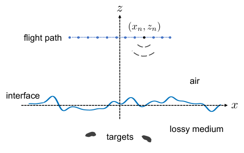
Figure 1: A sketch of the subsurface synthetic aperture imaging system. A platform moves along a prescribed flight path producing a synthetic aperture above an interface separating air from a lossy medium. The platform emits a signal and records the echoes including ground bounce signals due to reflections by the interface and scattered signals by the targets. The objective for the imaging problem is to identify and locate the subsurface targets.

For this problem, the signal emitted from the platform propagates down to the interface. Part of the signal is reflected by the interface which is called the ground bounce signal. The portion of that ground bounce signal that reaches the platform is recorded. Another part of the signal is transmitted across the interface and is incident on the subsurface targets which then scatter that signal. Since the medium below the interface is lossy, the power in the signals incident on and scattered by the targets is attenuated. A portion of that attenuated scattered signal is transmitted across the interface and propagates up to the platform where it is also recorded. Measurements are therefore comprised of ground bounce and scattered signals reaching the platform.

Using these measurements we seek to solve the inverse scattering problem that identifies and locates targets in the lossy medium below the interface. The medium above the interface is uniform and lossless and we assume that it is known. The medium below is also uniform, but lossy, so it has a complex relative dielectric permittivity. We assume we know the real part of the relative dielectric permittivity, but not its imaginary part corresponding to the absorption in the medium. Finally, the interface between the two media is unknown, but we assume that we know its mean, which is constant.

There are several key challenges to consider for this problem. Measurements include ground bounce and scattered signals. The ground bounce signals have more power than the scattered signals, but do not contain information about the targets. Thus, one needs an effective method to remove the ground bounce from measurements. Because the interface is uncertain, it is important to remove these ground bounce signals without requiring explicit knowledge of the interface location. Once that issue can be adequately addressed, we then require high-resolution images of the targets in an unknown, lossy medium obtained through solution of the inverse scattering problem. The absorption in the medium will limit the depth at which one can reliably solve the inverse scattering problem. However, we are interested in identifying targets that are located superficially below the interface, so the penetration depths needed for this problem are not too prohibitive. In addition, measurements are corrupted by additive measurement noise. Another noteworthy issue is that removal of the ground bounce signal from measurements will effectively increase the relative amount of noise in what remains which will limit the values of the signal-to-noise ratio (SNR) for which imaging will be effective.

3 Rough surface scattering

We model uncertainty in the interface separating the two media using random rough surfaces. In particular, we consider Gaussian-correlated random surfaces that are characterized by the RMS height, $h_{\text{RMS}}$ and the correlation length, $\ell$. In what follows, we give the integral equation formulation for computing reflection and transmission of signals across one realization of a random rough surface.

Let $z=h(x)$ for $-\infty<x<\infty$ denote one realization of the random rough surface separating two different media. The medium in $z>h(x)$ is uniform and lossless. The medium in $z<h(x)$ is also uniform, but lossy with relative dielectric constant $\epsilon_{r}(1+\mathrm{i}\beta)$ with $\epsilon_{r}$ denoting the real part of the relative dielectric constant and $\beta\geq 0$ denoting the loss tangent (ratio of the imaginary part over the real part of the relative dielectric constant). We consider two problems in which a point source is either above or below the interface. In what follows we assume that the total field and its normal derivative are continuous on $z=h(x)$ and that those fields satisfy appropriate out-going conditions as $z\to\pm\infty$.

3.1 Integral equations formulation

Suppose a point source is located at $(x_{0},z_{0})$ with $z_{0}>h(x_{0})$. Using Green’s second identity, we write

$$u(x,z)=G_{0}(x,z;x_{0},z_{0})+\mathscr{D}_{0}[U](x,z)-\mathscr{S}_{0}[V](x,z),\quad z>h(x),$$ (1)

with

$$\mathscr{D}_{0}[U](x,z)=\int_{-\infty}^{\infty}\frac{\partial G_{0}(x,z;\xi,h(\xi))}{\partial n}\sqrt{1+(h^{\prime}(\xi))^{2}}U(\xi)\mathrm{d}\xi,$$

and

$$\mathscr{S}_{0}[V](x,z)=\int_{-\infty}^{\infty}G_{0}(x,z;\xi,h(\xi))V(\xi)\mathrm{d}\xi.$$

Here,

$$G_{0}(x,z;x^{\prime},z^{\prime})=\frac{\mathrm{i}}{4}H_{0}^{(1)}\left(k_{0}\sqrt{(x-x^{\prime})^{2}+(z-z^{\prime})^{2}}\right),$$

with $k_{0}=\omega/c$ and

$$\frac{\partial G_{0}(x,z;\xi,\zeta)}{\partial n}\sqrt{1+(h^{\prime}(\xi))^{2}}=h^{\prime}(\xi)\frac{\partial G_{0}(x,z;\xi,\zeta)}{\partial\xi}-\frac{\partial G_{0}(x,z;\xi,\zeta)}{\partial\zeta}.$$ (2)

In addition, we have

$$v(x,z)=-\mathscr{D}_{1}[U](x,z)+\mathscr{S}_{1}[V](x,z),\quad z<h(x),$$ (3)

with $\mathscr{D}_{1}$ and $\mathscr{S}_{1}$ defined the same as $\mathscr{D}_{0}$ and $\mathscr{S}_{0}$, but with $G_{0}$ replaced with

$$G_{1}(x,z;x^{\prime},z^{\prime})=\frac{\mathrm{i}}{4}H_{0}^{(1)}\left(k_{1}\sqrt{(x-x^{\prime})^{2}+(z-z^{\prime})^{2}}\right),$$

and $k_{1}=k_{0}\sqrt{\epsilon_{r}(1+\mathrm{i}\beta)}$. Now, suppose a point source is located at $(x_{1},z_{1})$ with $z_{1}<h(x_{1})$. For that case we have

$$u(x,z)=\mathscr{D}_{0}[U](x,z)-\mathscr{S}_{0}[V](x,z),\quad z>h(x),$$ (4)

and

$$v(x,z)=G_{1}(x,z;x_{1},z_{1})-\mathscr{D}_{1}[U](x,z)+\mathscr{S}_{1}[V](x,z),\quad z<h(x).$$ (5)

The fields $u$ defined by either (1) or (4), and $v$ defined by either (3) or (5) are given in terms of surface fields $U(\xi)$ and $V(\xi)$. Physically, $U(\xi)=u(\xi,h(\xi))$ is the evaluation of the field on the interface point, $(\xi,h(\xi))$. The field $V(\xi)$ is defined in terms of the normal derivative of $u$ according to

$$V(\xi)=\sqrt{1+(h^{\prime}(\xi))^{2}}\frac{\partial u(\xi,h(\xi))}{\partial n}=h^{\prime}(\xi)\frac{\partial u(\xi,\zeta)}{\partial\xi}-\frac{\partial u(\xi,\zeta)}{\partial\zeta}.$$

These formulations given above make use of the aforementioned assumption that both $u$ and $\partial_{n}u$ are continuous on the interface $z=h(x)$.

The surface fields $U$ and $V$ are not yet determined. To determine them we evaluate $u$ and $v$ in the limit as $(x,z)\to(\xi,h(\xi))$ from above and below, respectively. In that limit, the $\mathscr{D}_{0}$ and $\mathscr{D}_{1}$ operators produce a jump and the result is a system of boundary integral equations. For the fields defined by (1) and (3), the resulting system is

$$\frac{1}{2}U(\xi)-\mathscr{D}_{0}[U](\xi)+\mathscr{S}_{0}[V](\xi) =G_{0}(\xi,h(\xi);x_{0},z_{0}),$$ (6a)

$$\frac{1}{2}U(\xi)+\mathscr{D}_{1}[U](\xi)-\mathscr{S}_{1}[V](\xi) =0,$$ (6b)

and for the fields defined by (4) and (5), the resulting system is

$$\frac{1}{2}U(\xi)-\mathscr{D}_{0}[U](\xi)+\mathscr{S}_{0}[V](\xi) =0,$$ (7a)

$$\frac{1}{2}U(\xi)+\mathscr{D}_{1}[U](\xi)-\mathscr{S}_{1}[V](\xi) =G_{1}(\xi,h(\xi);x_{1},z_{1}).$$ (7b)

The solution of each of these systems results in the determination of $U$ and $V$ for their respective problem. Once those are determined, the fields above and below the interface are computed through evaluation of (1) and (3) when the source is above the interface, or (4) and (5) when the source is below the interface. We give the numerical method we use to solve these systems in the Appendix.

3.2 Enhanced backscattering

The bistatic cross-section $\sigma(\theta_{s},\theta_{i})$ is the fraction of power reflected in the far field by the rough surface in direction $(\sin\theta_{s},\cos\theta_{s})$ with $\theta_{s}$ denoting the scattered angle made with respect to the $z$-axis due to a plane wave incident in direction $(\sin\theta_{i},-\cos\theta_{i})$ with $\theta_{i}$ denoting the angle of incidence. Reflection by the random rough surface makes up an important component of measurements in this imaging problem. Here, we use the bistatic cross-section to characterize reflection by the rough surface over the range of frequencies: $3.1$ GHz to $5.1$ GHz. We use the method given in (Tsang ., 2004, Chapter 4) to generate these rough surfaces and compute the corresponding bistatic cross-sections. We then average over several realizations of the rough surface to determine canonical features of these rough surfaces.

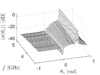
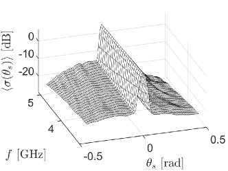
Figure 2: [Left] Average of the bistatic cross-section, $\langle\sigma(\theta_{s},\theta_{i})\rangle$, over $100$ realizations of a Gaussian-correlated random rough surface with $h_{\text{RMS}}=0.2$ cm and $\ell=8$ cm due to a plane wave incident with $\theta_{i}=30$ degrees. [Right] A close-up of this result about $\theta_{s}=\theta_{i}$.

In Fig. 2 we show the bistatic cross-section due to a plane wave with $\theta_{i}=30$ degrees averaged over $100$ realizations of a Gaussian-correlated rough surface with RMS height $h_{\text{RMS}}=0.2$ cm and correlation length $\ell=8$ cm. These results show a sharp angular cone about $\theta_{s}=\theta_{i}$ as a consequence of enhanced backscattering. Enhanced backscattering is a canonical multiple scattering phenomenon in which counter-propagating scattered waves add coherently in the retro-reflected direction, $\theta_{s}=\theta_{i}$.

With these surface roughness parameters, we find that scattering by the random rough surface is significant and cannot be ignored. Because these rough surfaces exhibit enhanced backscattering, there is significant multiple scattering. Moreover, SAR measurements use a single emitter/receiver, so we measure the field exactly at the retro-reflected angle corresponding to the peak of the angular cone. However, we do not care to reconstruct this rough surface profile for this imaging problem. Rather, we seek a method that attempts to identify and locate targets without needing to consider this rough surface. Nonetheless, scattering by the rough surface will be an important factor in the measurements.

4 Modeling measurements

In this work we consider scattering by subsurface point targets. This assumption simplifies the modeling of measurements which, in turn, enables the determination of the effectiveness of a subsurface imaging method. We consider imaging point targets here as a necessary first problem for any effective imaging method to solve.

To model measurements we must consider both the ground bounce signal that is the reflection by the rough surface, and the scattered signal by the targets. Assuming that scattering by each target is independent from any others, we give the procedure we use to model measurements for a single point target located at $(x_{1},z_{1})$ below due to a point source located at $(x_{0},z_{0})$.

1. Compute one realization of the Gaussian-correlated rough surface, $z=h(x)$, with RMS height $h_{\text{RMS}}$ and correlation length $\ell$.

2. Solve the system (6). Let $U_{0}$ and $V_{0}$ denote the solution.

3. Compute the ground-bounce signal, $R$, through evaluation of

   $$R=\mathscr{D}_{0}[U_{0}](x_{0},z_{0})-\mathscr{S}_{0}[V_{0}](x_{0},z_{0}).$$

   This expression is the field reflected by the rough surface evaluated at the same location as the source.

4. Solve the system (7). Let $U_{1}$ and $V_{1}$ denote the solution.

5. Compute the field scattered by the point target, $S$, through evaluation of

   $$S=\left(\mathscr{D}_{0}[U_{1}](x_{0},z_{0})-\mathscr{S}_{0}[V_{1}](x_{0},z_{0})\right)\rho\left(-\mathscr{D}_{1}[U_{0}](x_{1},z_{1})+\mathscr{S}_{1}[V_{0}](x_{1},z_{1})\right).$$

   There are three factors in this expression written in right-to-left order just like matrix products. The third factor corresponds to the field emitted from the source that transmits across the interface and is incident on the target. The second factor is the reflectivity of the target $\rho$. The first factor is the propagation of the second and third terms from the target location to the receiver location.

Steps 2 through 5 of this procedure are repeated over each frequency $\omega_{m}$ for $m=1,\dots,M$ and each spatial location of the platform $\boldsymbol{x}_{n}$ for $n=1,\dots,N$. The results are $M\times N$ matrices $R$ and $S$. When there are multiple targets, we repeat Steps 4 and 5 for each of the targets and $S$ is the sum of those results.

Using this procedure above, we model measurements according to

$$D=R+S+\eta,$$ (8)

with $\eta$ denoting additive measurement noise which we model as Gaussian white noise. The inverse scattering problem is to identify targets and determine their locations from the data matrix $D$.

5 Ground bounce signal removal

According to measurement model (8), the ground bounce signal $R$ is added to the scattered signal $S$. The ground bounce signal does not contain any information about the targets. Since we do not seek to reconstruct the interface for this imaging problem, $R$ impedes the solution of the inverse scattering problem. Hence, we seek to remove it from measurements.

The key assumption we make is that the relative amount of power in $R$ is larger than that in $S$. This assumption opens the opportunity to use principal component analysis to attempt to remove $R$ from $D$. Let $D=U\Sigma V^{H}$ denote the singular value decomposition of $D$ where $V^{H}$ denotes the Hermitian or conjugate transpose of $V$. Because of uncertainty in the interface, we are not able to explicitly determine the structure of the singular values $\sigma_{j}$ for $j=1,\dots,\min(M,N)$ in the $M\times N$ diagonal matrix $\Sigma$. Instead we seek to observe any changes in the spectrum of singular values that indicate a separation between contributions by $R$ and $S$.

Consider $M=25$ frequencies uniformly sampling the bandwidth ranging from $3.1$ GHz to $5.1$ GHz and $N=21$ spatial locations of the platform uniformly sampling the aperture $a=1$ m at $1$ m above the mean interface height $\langle h(x)\rangle=0$. We set $\epsilon_{r}=9$ and $\beta=0.1$. Using one realization of a rough surface with $h_{\text{RMS}}=0.2$ cm and $\ell=8$ cm, we compute $R$. Then we compute the SVD of $R$ and examine the singular values.

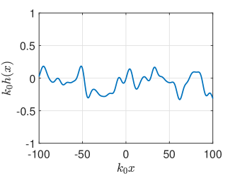
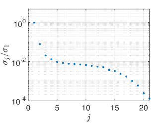
Figure 3: [Left] One realization of the Gaussian-correlated random rough surface with $h_{\text{RMS}}=0.2$ cm and $\ell=8$ cm with $k_{0}$ denoting the wavenumber at the central frequency. [Right] The singular values of the ground bounce signals by this rough surface normalized by the first singular value $\sigma_{1}$.

In Fig. 3 we show results for one realization of the Gaussian-correlated rough surface with $h_{\text{RMS}}=0.2$ cm and $\ell=8$ cm shown in the left plot and the corresponding singular values (normalized by the first singular value, $\sigma_{1}$) for the resulting ground bounce signals in the right plot. Note that this realization of the rough surface is one among those used to study the bistatic cross-section in Fig. 2 which exhibited enhanced backscattering. Consequently, we know that the ground bounce signals include strong multiple scattering by the rough surface.

Looking at the singular values in Fig. 3 we identify a change in behavior in their decay. From $j=1$ to $j=5$, we find that $\sigma_{j}$ decays rapidly over two orders of magnitude. In contrast, from $j=6$ to $j\approx 15$, we find that the decay of $\sigma_{j}$ is much slower and then decays thereafter. We have observed that this qualitative behavior of the singular values persists over different realizations.

Through these observations of the behavior of singular values for $R$, we now propose a method to approximately remove $R$ from $D$ given as the following procedure.

1. Compute the SVD of the measurement matrix $D=U\Sigma V^{H}$.

2. Identify the index $j^{\ast}$ where the rapid decay of the singular values stops and the behavior changes.

3. Compute

   $$\tilde{D}=D-\sum_{i=1}^{j^{\ast}}\sigma_{i}\mathbf{u}_{i}\mathbf{v}_{i}^{H},$$ (9)

   where $\mathbf{u}_{i}$ and $\mathbf{v}_{i}$ denote the $i$-th columns of $U$ and $V$, respectively.

It is likely that this procedure does not remove $R$ from $D$ exactly. However, we apply this procedure to obtain $\tilde{D}$ and test below if this procedure works well enough for identifying and locating targets.

Note that measurement noise is applied to $D=R+S$. The corresponding SNR is defined according to $\text{SNR}=10\log_{10}(\|R+S\|_{F}/\|\eta\|_{F})$ with $\|\cdot\|_{F}$ denoting the Frobenius norm. This SNR is dominated by $R$ since $\|R\|_{F}\gg\|S\|_{F}$. When we remove $R$ from $D$, there will be an effective SNR ($\text{eSNR}=10\log_{10}(\|S\|_{F}^{2}/\|\eta\|_{F}^{2})$) based on $S$ which will be much lower. For this reason, we see that this subsurface imaging problem is more sensitive to noise than other imaging problems where ground bounce signals are not present.

6 Kirchhoff migration imaging

Consider a sub-region of $z<h(x)$ where we seek to form an image. We call this sub-region the imaging window (IW). Let $(x,z)\in\mathrm{IW}$ denote a search point in the IW. To form an image which identifies targets and gives estimates for their locations, we evaluate the KM imaging functional,

$$I^{\text{KM}}(\boldsymbol{y})=\left|\sum_{m=1}^{M}\sum_{n=1}^{N}\tilde{d}_{mn}a_{mn}^{\ast}(x,z)\right|,$$ (10)

over a mesh of grid points sampling the IW. Here $\tilde{d}_{mn}$ is the $(m,n)$ entry of the matrix $\tilde{D}$ and $a_{mn}(x,z)$ are called the illuminations. The superscript ^∗ denotes the complex conjugate. The illuminations effectively back-propagate the data so that the resulting image formed shows peaks on the target locations.

6.1 Computing illuminations

To compute the illuminations $a_{mn}(x,z)$ we first note that we do not know the interface $z=h(x)$ nor do we seek to reconstruct it. However, we assume that $\langle h(x)\rangle=0$ is known, so we consider the interface $z=0$ instead. Additionally, we do not know the loss tangent $\beta$ that dictates the absorption in the lower medium. In fact, we have shown previously that making use of any knowledge of the absorption is not useful for imaging to identify and locate targets Kim  Tsogka (20231). However, we assume that $\epsilon_{r}$ is known. With these assumptions, we write

$$a_{mn}(x,z)=\phi^{(0)}_{mn}(x,z)\phi^{(1)}_{mn}(x,z).$$ (11)

Here, $\phi^{(0)}_{mn}(x,z)$ corresponds to the field on $(x,z)$ due to a point source with frequency $\omega_{m}$ located at $\boldsymbol{x}_{n}$ whose amplitude is normalized to unity. The quantity $\phi^{(1)}_{mn}(x,z)$ is the field with frequency $\omega_{m}$ evaluated on $\boldsymbol{x}_{n}$ due to a point source at $(x,z)$ whose amplitude is normalized to unity.

Using Fourier transform methods, we find that the field $u^{(0)}$ evaluated on $(x,z)$ due to a point source with frequency $\omega_{m}$ located at $\boldsymbol{x}_{n}=(x_{n},z_{n})$ is

$$u^{(0)}=\frac{\mathrm{i}}{2\pi}\int\frac{e^{\mathrm{i}(q_{0}z_{n}-q_{1}z)}}{q_{0}+q_{1}}e^{\mathrm{i}\xi(x-x_{n})}\mathrm{d}\xi,$$ (12)

with $q_{0}=\sqrt{\omega_{m}^{2}/c^{2}-\xi^{2}}$ and $q_{1}=\sqrt{\epsilon_{r}\omega_{m}^{2}/c^{2}-\xi^{2}}$. Similarly, we find that the field $u^{(1)}$ evaluated on $(x_{n},z_{n})$ due to a ponit source with frequency $\omega_{m}$ located at $(x,z)$ is

$$u^{(1)}=\frac{\mathrm{i}}{2\pi}\int\frac{e^{\mathrm{i}(q_{0}z_{n}-q_{1}z)}}{q_{0}+q_{1}}e^{\mathrm{i}\xi(x_{n}-x)}\mathrm{d}\xi.$$ (13)

Upon computing $u^{(0)}$ and $u^{(1)}$, we evaluate $\phi_{mn}^{(0)}=u^{(0)}/|u^{(0)}|$ and $\phi_{mn}^{(1)}=u^{(1)}/|u^{(1)}|$.

Both $u^{(0)}$ and $u^{(1)}$ are integrals of the form,

$$I=\int_{-\infty}^{\infty}\frac{f(\xi)}{\sqrt{k_{0}^{2}-\xi^{2}}+\sqrt{k_{1}^{2}-\xi^{2}}}e^{\mathrm{i}\beta_{1}\sqrt{k_{0}^{2}-\xi^{2}}+\mathrm{i}\beta_{2}\sqrt{k_{1}^{2}-\xi^{2}}}e^{\mathrm{i}\xi\gamma}\mathrm{d}\xi,$$ (14)

with $k_{1}=k_{0}\sqrt{\varepsilon_{r}}$, and $\beta_{1}$, $\beta_{2}$, and $\gamma$ denoting real parameters. The wavenumbers $k_{0}$ and $k_{1}$ are real, and we assume that $|k_{0}|<|k_{1}|$. This Fourier integral, which is one example of a Sommerfeld integral, is notoriously difficult to compute due to the highly oscillatory behavior of the function inside the integral. There have been several approaches to compute this Fourier integral accurately Cai (2002); O’Neil . (2014); Bruno . (2016). To compute (14), we follow Barnett  Greengard (2011) and integrate on a deformed contour in the complex plane to avoid branch points. Here, we use the deformed contour

$$\xi(s)=s+\mathrm{i}A\left[e^{-w(s+k_{0})^{2}}+e^{-w(s+k_{1})^{2}}-e^{-w(s-k_{0})^{2}}-e^{-w(s-k_{1})^{2}}\right],$$

with $-\infty<s<\infty$, and $A$ and $w$ denoting user-defined parameters. Integration is taken with respect to $s$ over a truncated, finite interval chosen so that the truncation error is smaller than the finite precision arithmetic. In the simulations that follow, we have used $500$ quadrature points with $A=0.4$ and $w=6$. We also use the suggestion in Barnett  Greengard (2011) of applying the mapping $s=\sinh(\beta)$ with $-\infty<\beta<\infty$ to cluster quadrature points in the interval $(-k_{0},k_{0})$.

6.2 Modified KM

We have recently developed a modification to KM that allows for tunably high-resolution images of individual targets Kim  Tsogka (20233). Suppose that we have evaluated (10) and identified a target. In a region about that target, we normalize $I^{\mathrm{KM}}$ so that its peak value is $1$. Let $\bar{I}^{\mathrm{KM}}$ denote the normalization of $I^{\mathrm{KM}}$ in this region. With this normalized image, we compute the following Möbius transformation,

$$I_{\delta}^{\text{KM}}(\boldsymbol{y})=\frac{\delta}{1-(1-\delta)\bar{I}^{\mathrm{KM}}(\boldsymbol{y})},$$ (15)

with $\delta>0$ denoting a user-defined tuning parameter. We call the resulting image formed with (15) the modified KM image. In the whole space, we have determined that this modified KM method scales the resolution of KM by $\sqrt{\delta}$. Because $\delta$ is a user-defined quantity, it can be set to be arbitrarily small. It is in this way that $I_{\delta}^{\text{KM}}$ produces tunably high-resolution images of targets.

7 Numerical results

We now present numerical results where we have (i) simulated measurements using the procedure given in Section 4, (ii) removed the ground bounce signal using the procedure given in Section 5, and then produced images through evaluation of the KM and modified KM imaging functions given in Section 6.

Just as we have done for the results shown in Section 5, we have used $M=25$ frequencies uniformly sampling the bandwidth ranging from $3.1$ GHz to $5.1$ GHz and $N=21$ spatial locations of the platform uniformly sampling the aperture $a=1$ m situated $1$ m above the average interface height $\langle h(x)\rangle=0$. We set $\epsilon_{r}=9$ and $\beta=0.1$ as suggested by Daniels for modeling buried landmines Daniels (2006). We compute imaging results for one realization of a Gaussian-correlated rough surface that has $h_{\text{RMS}}=0.2$ cm and $\ell=8$ cm.

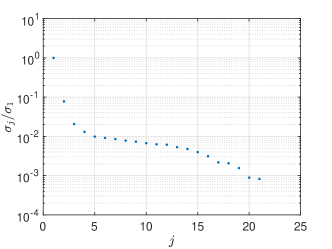
Figure 4: Singular values of the matrix $D$. These measurements include the ground bounce signals by one realization of a Gaussian-correlated rough surface with $h_{\text{RMS}}=0.2$ cm and $\ell=8$ cm. Additionally, they include scattering by a point target located at $(2,-8)$ cm with $\rho=3.4\mathrm{i}$. Measurement noise has been added so that $\text{SNR}=24.2$ dB.

7.1 Single target

Let the origin of a coordinate system correspond to the center of the flight path in the $x$-coordinate and the mean surface height $\langle h(x)\rangle=0$ in the $z$-coordinate as shown in Fig. 1. We compute images for a target located at $(2,-8)$ cm with reflectivity $\rho=3.4\mathrm{i}$. Measurement noise is added to the simulated measurements so that $\text{SNR}=24.2$ dB.

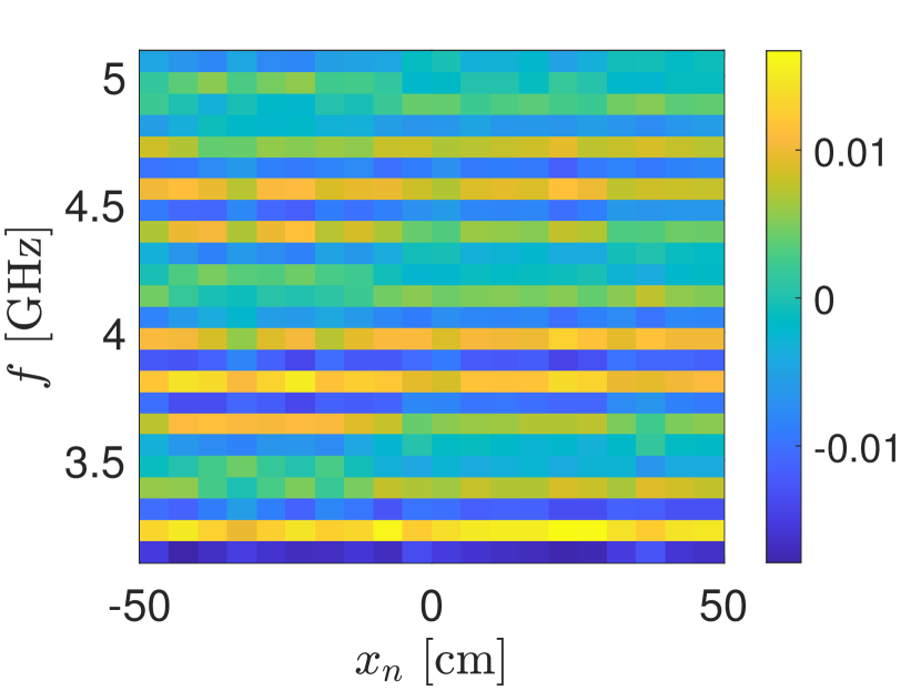
(a) $D$

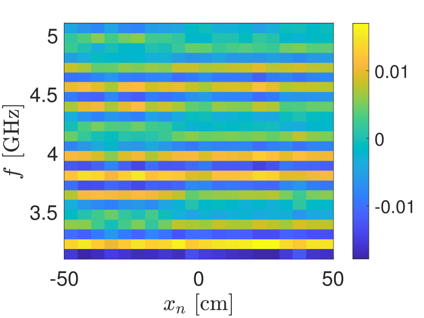
(b) $R$

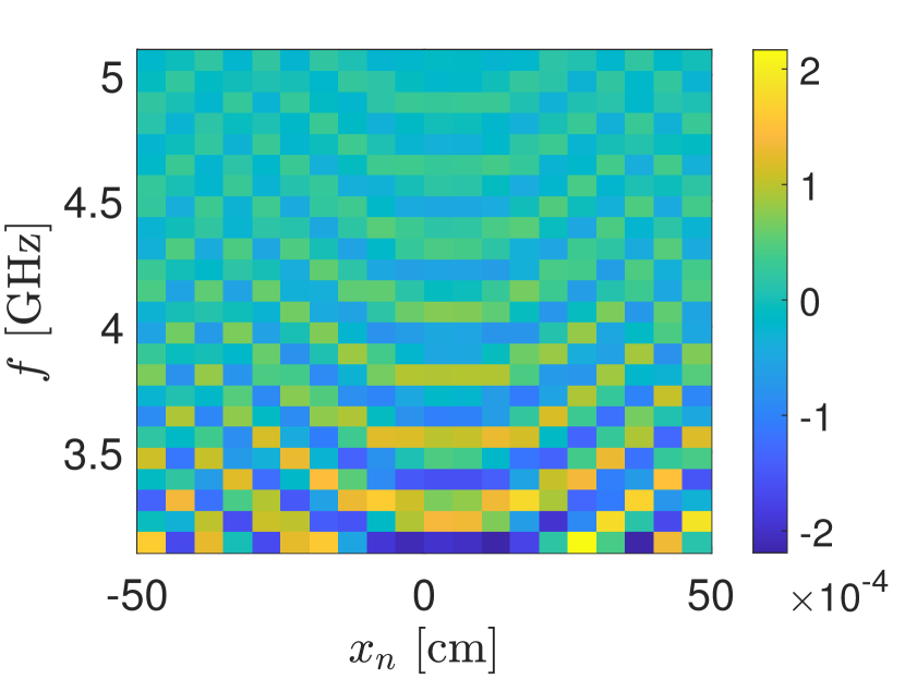
(c) $S$

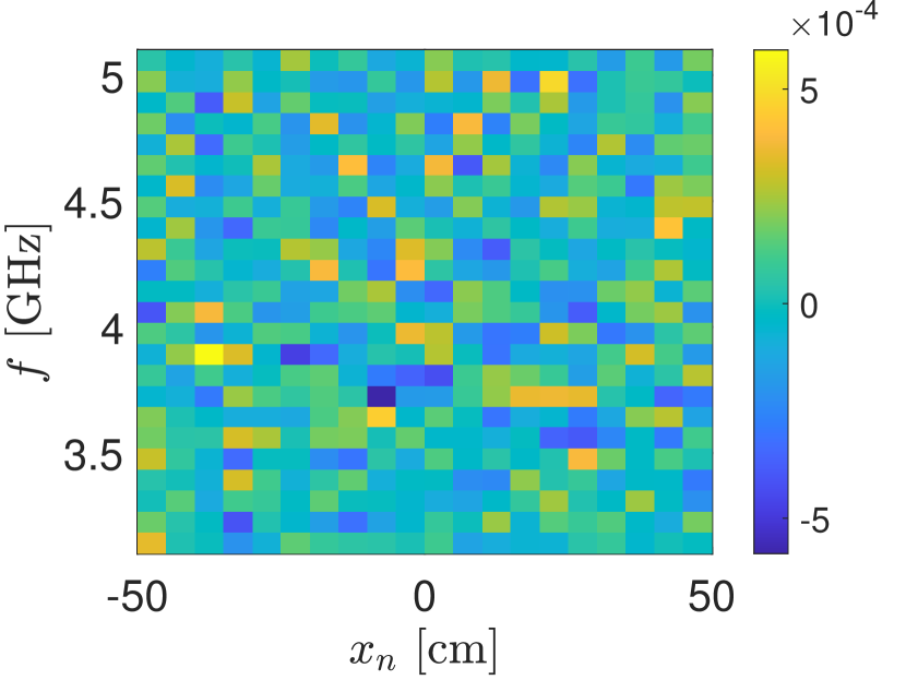
(d) $\tilde{D}$

Figure 5: Real part of the entries of (a) the data matrix $D$, (b) the ground bounce signals $R$, (c) the scattered signals $S$, and (d) the matrix $\tilde{D}$ with the contributions from the first $5$ singular values removed.

Figure 4 shows the singular values for the data matrix $D$ normalized by the first singular value. Similar to what we observed in Section 5 with the ground bounce signals, we find that the first $5$ singular values decay rapidly. The singular values $\sigma_{j}$ for $j>5$ show a different behavior. Thus, we apply the ground bounce removal procedure given in Section 5 using $j^{\ast}=5$.

We show real part of the data matrix $D$ in the top left plot of Fig. 5. In the top right plot of Fig. 5 we show the real part of the ground bounce signals in $R$. Note that the plots for $D$ and $R$ are nearly indistinguishable consistent with our assumption that the ground bounce signals dominate the measurements. In the bottom left plot of Fig. 5 we show the real part of the scattered fields in $S$. Note that those values in $S$ are nearly $2$ orders of magnitude smaller than those of $R$. The bottom right plot shows the real part of $\tilde{D}$ resulting from removing the contributions from the first $j^{\ast}=5$ singular values. While the magnitudes of the values in $S$ and $\tilde{D}$ are comparable, they appear qualitatively different from one another. Thus, it is unclear from these results whether or not $\tilde{D}$ contains information regarding the target.

In Fig. 6 we apply KM (center plot) and the modified KM with $\delta=10^{-2}$ (right plot) to $\tilde{D}$. For reference, we have also included the result of applying KM to $S$ in the left plot of Fig. 6. This ideal case represents exact ground bounce removal. Despite the fact that the results for $S$ and $\tilde{D}$ in Fig. 5 were not qualitatively similar, the corresponding KM images in Fig. 6 are quite similar in the vicinity of the target and show peaks about the target location, $(2,-8)$cm. The peak of the KM image (center) is accompanied by several imaging artifacts away from the target location. In contrast, by applying the modified KM method we eliminate those artifacts and obtain a high resolution image of the target. We note that the predicted location determined from where the KM and modified KM images attain their peak value on the meshed used to plot them is $(1.5,-8.2)$ cm, which is slightly shifted from the true location. Nonetheless, this result is quite good given the uncertainty in the surface, the inexact method for ground bounce removal, unknown absorption, and substantial measurement noise in the system.

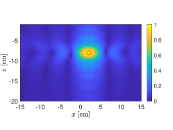
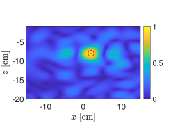
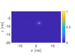
Figure 6: [Left] The ideal imaged formed through evaluation of the KM imaging function (10) applied to the scattered signals contained in $S$. [Center] The image formed through evaluation of (10) applied to $\tilde{D}$. [Right] The imaged formed through evaluation of the modified KM imaging function (15) with $\delta=10^{-2}$ applied to the KM image in the center. In each of the plots, the exact target location is plotted as a red “$\odot$” symbol.

The unknown absorption puts a depth limitation on imaging targets. When the target depth is comparable to the absorption length, the imaging method is not able to distinguish between the true target and a weaker target less deep in the medium. We have observed this phenomenon with optical diffusion González-Rodríguez . (2018). Here, uncertainty in the rough surface complicates this situation even further. In Fig. 7 we show KM and modified KM ($\delta=10^{-2}$) images for a target located at $(2,-12)$ cm (top row) and for a target located at $(2,-16)$ cm. As the target is placed deeper into the medium, we observe an increase in the KM imaging artifacts. For the target located $12$ cm below the surface, we find that these imaging artifacts contain the peak value of the function and the target is no longer identifiable in the image. The modified KM images clearly show this behavior.

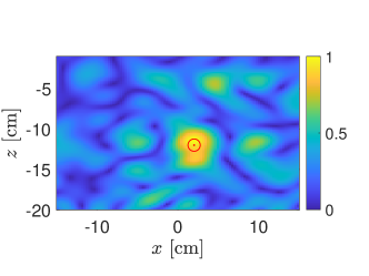
(a) Target located at $(x,z)=(2,-12)$ cm.

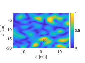
(b) Target at $(x,z)=(2,-16)$ cm.

Figure 7: [Left] The imaged formed through evaluation of the KM imaging function (10). The exact target location is plotted as a red “$\odot$” symbol. [Right] The imaged formed through evaluation of the modified KM imaging function (15) with $\delta=10^{-2}$. The top row is for a target located at $(2,-12)$ cm and the bottom row is for a target located at $(2,-16)$ cm.

The inability of the imaging method to identify targets deep in the medium is either due to the absorption, the uncertainty of the rough surface, some combination of these, or possibly other factors. In Fig. 8 we show the resulting image for a target located at $(2,-16)$ cm with the reduced loss tangent, $\beta=0.05$. All other parameters are the same as those used in the previous images. With this reduced loss tangent, we find that KM and the modified KM are clearly able to identify the target. From this result we conclude that the absorption is the main factor limiting the range of target depths for this imaging method.

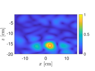
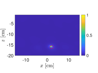
Figure 8: The same as Fig. 7(b) except that the absorption is reduced from the previous results with $\beta=0.05$.

As we explained above, when we remove ground bounce signals, we introduce an effective SNR (eSNR) that is important for subsurface imaging. We expect that KM will be effective as long as $\text{eSNR}>0$ dB. For the results shown in Fig. 6, $\text{SNR}=24.2$ dB and $\text{eSNR}=3.0$ dB. The resulting image clearly identifies the target and accurately predicts its location. In contrast, we show results for $\text{SNR}=14.2$ dB and $\text{eSNR}=-7.0$ dB in Fig. 9. This image has several artifacts that dominate over any peak formation about the target location. It is important to note that the eSNR that we use here cannot be estimated a priori. This result demonstrates that SNR demands on imaging systems are higher for subsurface imaging problems than other imaging problems that do not involve ground bounce signals.

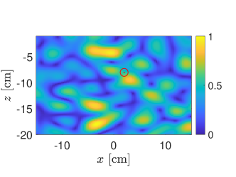
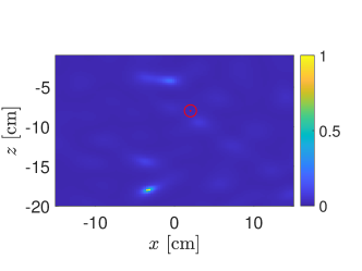
Figure 9: [Left] KM image and [Right] modified KM image with $\delta=10^{-2}$ for a target located at $(2,-8)$ cm with $\text{SNR}=14.2$ dB and $\text{eSNR}=-7.0$ dB.

7.2 Multiple targets

We now consider imaging regions with $3$ targets. Target $1$ is located at $(-9.0,10.1)$ cm with reflectivity $\rho_{1}=3.6\mathrm{i}$, target $2$ is located at $(1.0,-9.4)$ cm with reflectivity $\rho_{2}=3.4\mathrm{i}$ and target $3$ is located at $(11.0,-9.8)$ cm with reflectivity $\rho_{3}=3.6\mathrm{i}$. The measurements were computed using the procedure given in Section 4. Measurement noise has been added so that $\text{SNR}=24.2$ dB.

The result from evaluating the KM imaging function (10) for this problem is shown in the left figure of Fig. 10. The corresponding result from evaluating the modified KM imaging function (15) with $\delta=10^{-2}$ is shown in the right plot of Fig. 10. These images show that the method is capable of identifying the three targets and give good predictions for their locations.

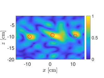
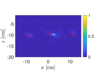
Figure 10: [Left] The imaged formed through evaluation of the KM imaging function (10) for three targets. The exact target locations are plotted as a red “$\odot$” symbol. [Right] The image formed through evaluation of the modified KM imaging function (15) with $\delta=10^{-2}$. Measurement noise is added so that $\text{SNR}=24.2$ dB.

The result from the modified KM method does not show the three targets equally clearly. In fact, the peak formed near target 2 is the strongest in the KM image, so the result for the modified KM image shows target 2 most clearly. This is because the normalization of the KM image required for evaluating the modified KM image is based on target 2. As an alternative, we consider $5\,\text{cm}\,\times\,5\,\text{cm}$ sub-regions about each of the peaks of the KM image. Within each of those sub-regions, we normalize the KM image and evaluate the modified KM image with $\delta=10^{-2}$. Those results are shown in Fig. 11. Each of those sub-region images is centered about the corresponding exact target location and scaled by the central wavenumber $k_{0}$. Even though the predicted target locations are shifted from the exact target location, these results show that these shifts are small fractions of the central wavelength.

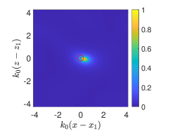
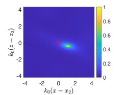
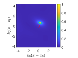
Figure 11: Evaluation of the modified KM imaging function (15) with $\delta=10^{-2}$ in sub-regions centered about each target location.

These results show that this imaging method is capable of identifying multiple targets. However, there are limitations. The targets cannot be too close to one another due to the finite resolution of KM imaging. Moreover, due to absorption in the medium, there are depth limitations to where targets can be identified. Additionally, when there are multiple targets at different depths, it is likely that those targets that are deeper than others may be not be identifiable in images.

8 Conclusions

We have discussed synthetic aperture subsurface imaging of point targets. Here, we have modeled uncertainty about the interface between the two media with Gaussian-correlated random rough surfaces characterized by a RMS height and correlation length. The medium above the interface is uniform and lossless. The medium below the interface is uniform and lossy. The loss tangent of the medium below the interface is not known when imaging.

The imaging method involves two steps. First, we attempt to remove ground bounce signals using principal component analysis. This method does not require any explicit information about the interface other than the ground bounce signals is stronger than the scattered signals. There is no a priori method to choose the number of principal components to include in the ground bounce removal procedure. Instead, we have proposed to determine where the decay of the singular values changes behavior and use that for the grounce bounce removal procedure. Using the resulting matrix after removing the ground bounce signal, we apply Kirchhoff migration (KM) and our modification to it that allows for tunably high resolution images of targets. In our implementation of KM imaging, we compute so-called illuminations for the problem with a flat interface at the mean interface height using only the real part of the relative dielectric permittivity for the medium below that interface, so we completely neglect the unknown absorption in the medium.

Our numerical results show that despite uncertainty in the interface, the inexactness of the ground bounce removal procedure, unknown absorption, and measurement noise, this imaging method is able to identify and locate targets robustly and accurately. However, there are limitations to the capabilities of this imaging method. The main limitation for this imaging method is that targets cannot be too deep below the interface. Absorption attenuates the scattered power and depends on the path length of signals. When targets are deep below the interface, the path length of scattered signals are too large and attenuation renders those scattered signals undetectable within the dynamic range of measurements. Additionally, targets cannot be too closely situated to one another. The KM imaging method is limited in its resolution. If targets are situated closer than the resolution capabilities of KM, they cannot be distinguished.

Despite the limitations of this imaging method, we find these results to be a promising first step toward practical imaging problems. A key extension of this work will be to incorporate quantitative imaging methods that will open opportunities for target classification in addition to identification and location. We have recently developed methods for recovering the radar cross-section (RCS) for dispersive point targets when there is no ground bounce signal Kim  Tsogka (20232). Recovering the RCS for individual targets can be used to classify targets by properties related to their size or material properties when their shape or other geometrical features are not available for recovery. The challenge with quantitative imaging methods for this problem will be addressing both the unknown absorption and uncertain rough interface. As mentioned previously, absorption will attenuate the power scattered by targets. Moreover, it will attenuate power non-uniformly over frequency which introduces new challenges. The uncertainty in the rough interface also affects our ability to recover quantitative information. Because our method for removing ground bounce signals from an unknown rough surface is approximate, it yields errors in the phase which impeded the recovery of quantitative information. Developing extensions that allow for quantitative subsurface imaging is the subject of our future work.

Appendix: Numerical solution of the system of boundary integral equations

The method that we use to compute realizations of the Gaussian-correlated rough surface Tsang . (2004) uses discrete Fourier transforms, which assumes periodicity over the interval $[-L/2,L/2]$. The truncated domain width $L$ is chosen large enough so that edges do not strongly affect the results. In the simulations used here we set $L=4$ m compared to the $1$ m aperture and $30$ cm wide imaging window.

To compute the numerical solution of (6) or (7), we first truncate the integrals to the interval $-L/2\leq\xi\leq L/2$ and then replace those integrals with numerical quadrature rules. The result of this approximation is a finite dimensional linear system of equations suitable for numerical computation. Because the rough surfaces are periodic, we use the periodic trapezoid rule (composite trapezoid rule for a periodic domain). However, because the integral operators in (6) and (7) are weakly singular, we need to make modifications to the periodic trapezoid rule which we explain below.

We discuss the modification to the periodic trapezoid rule we use for the integrals,

$$I_{D}(s)=\int_{-L/2}^{L/2}\frac{\partial G(s,h(s);t,h(t))}{\partial n}\sqrt{1+(h^{\prime}(t))^{2}}U(t)\mathrm{d}t,$$ (A1)

and

$$I_{S}(s)=\int_{-L/2}^{L/2}G(s,h(s);t,h(t))V(t)\mathrm{d}t,$$ (A2)

with

$$G(s,h(s);t,h(t))=\frac{\mathrm{i}}{4}H_{0}^{(1)}\left(k\sqrt{(s-t)^{2}+(h(s)-h(t))^{2}}\right).$$

Let $t_{j}=-L/2+(j-1)\Delta t$ for $j=1,\dots,M$ denote the $M$ quadrature points with $\Delta t=L/M$. By applying the periodic trapezoid rule to (A1) and (A2) and evaluating that result on $s=t_{i}$, we obtain

$$I_{D}^{M}(t_{i})=\Delta t\sum_{j=1}^{M}\frac{\partial G(t_{i},h(t_{i});t_{j},h(t_{j}))}{\partial n}\sqrt{1+(h^{\prime}(t_{j}))^{2}}U(t_{j}),$$

and

$$I_{S}^{M}(t_{i})=\Delta t\sum_{j=1}^{M}G(t_{i},h(t_{i});t_{j},h(t_{j}))V(t_{j}).$$

Let $A$ be the $M\times M$ matrix whose entries are

$$a_{ij}=\Delta t\frac{\partial G(t_{i},h(t_{i});t_{j},h(t_{j}))}{\partial n}\sqrt{1+(h^{\prime}(t_{j}))^{2}},$$ (A3)

and let $B$ be the $M\times M$ matrix whose entries are

$$b_{ij}=\Delta tG(t_{i},h(t_{i});t_{j},h(t_{j})).$$ (A4)

With these matrices defined, the approximations for the integral operators given above are matrix-vector products. The problem with these results is that the kernels for $I_{D}^{M}$ and $I_{S}^{M}$ are singular on $t_{j}=t_{i}$, so the diagonal entries of $A$ and $B$ cannot be specified.

The modification to the periodic trapezoid rule we make is to replace the diagonal entries of $A$ and $B$ by

$$a_{ii}=U(t_{i})\int_{t_{i}-\Delta t/2}^{t_{i}+\Delta t/2}\frac{\partial G(t_{i},h(t_{i});t,h(t))}{\partial n}\sqrt{1+(h^{\prime}(t))^{2}}\mathrm{d}t,$$

and

$$b_{ii}=V(t_{i})\int_{t_{i}-\Delta t/2}^{t_{i}+\Delta t/2}G(t_{i},h(t_{i});t,h(t))\mathrm{d}t.$$

Note that we have assumed that $U(t)$ and $V(t)$ are approximately constant over this interval thereby allowing us to factor them out from the integral. Substituting $t=t_{i}+\tau$ and $\mathrm{d}t=\mathrm{d}\tau$, we obtain

$$a_{ii}=U(t_{i})\int_{-\Delta t/2}^{\Delta t/2}\frac{\partial G(t_{i},h(t_{i});t_{i}+\tau,h(t_{i}+\tau))}{\partial n}\sqrt{1+(h^{\prime}(t_{i}+\tau))^{2}}\mathrm{d}\tau,$$

and

$$b_{ii}=V(t_{i})\int_{-\Delta t/2}^{\Delta t/2}G(t_{i},h(t_{i});t_{i}+\tau,h(t_{i}+\tau))\mathrm{d}\tau.$$

Next, we evaluate the expressions involving $G$ and find that

$$\frac{\partial G(t_{i},h(t_{i});t_{i}+\tau,h(t_{i}+\tau))}{\partial n}\sqrt{1+(h^{\prime}(t_{i}+\tau))^{2}}\\ =-\frac{\mathrm{i}k}{4}\left[h^{\prime}(t_{i})\tau-h(t_{i})+h(t_{i}+\tau)\right]\frac{H_{1}^{(1)}(k\sqrt{\tau^{2}+(h(t_{i})-h(t_{i}+\tau))^{2}})}{\sqrt{\tau^{2}+(h(t_{i})-h(t_{i}+\tau))^{2}}},$$

and

$$G(t_{i},h(t_{i});t_{i}+\tau,h(t_{i}+\tau))=\frac{\mathrm{i}}{4}H_{0}^{(1)}(k\sqrt{\tau^{2}+(h(t_{i})-h(t_{i}+\tau))^{2}})$$

Expanding about $\tau=0$, we find

$$\frac{\partial G(t_{i},h(t_{i});t_{i}+\tau,h(t_{i}+\tau))}{\partial n}\sqrt{1+(h^{\prime}(t_{i}+\tau))^{2}}=\frac{h^{\prime\prime}(t_{i})}{4\pi(1+(h^{\prime}(t_{i}))^{2})}+O(\tau^{2}),$$

and

$$G(t_{i},h(t_{i});t_{i}+\tau,h(t_{i}+\tau))=\frac{1}{4\pi}\left[-2\gamma+\mathrm{i}\pi-2\log\left(\frac{1}{2}k|\tau|\sqrt{1+(h^{\prime}(t_{i}))^{2}}\right)\right]+O(\tau^{2}),$$

with $\gamma=0.5772\dots$ denoting the Euler-Mascheroni constant. Integrating these expressions over $-\Delta t/2\leq\tau\leq\Delta t/2$, we set

$$a_{ii}=\frac{\Delta t}{4\pi}\frac{h^{\prime\prime}(t_{i})}{1+(h^{\prime}(t_{i}))^{2}},$$ (A5)

and

$$b_{ii}=\frac{\Delta t}{2\pi}\left[1-\gamma+\mathrm{i}\frac{\pi}{2}-\log\left(\frac{1}{4}k\Delta t\sqrt{1+(h^{\prime}(t_{i}))^{2}}\right)\right].$$ (A6)

Thus, to form the matrix $A$, we evaluate (A3) for all $i\neq j$ and (A5) for $i=j$. Similarly, to form the matrix $B$, we evaluate (A4) for all $i\neq j$ and (A6) for $i=j$. With these matrices, we seek the vectors of unknowns, $\mathbf{u}=(U(t_{1}),\dots,U(t_{M}))$ and $\mathbf{v}=(V(t_{1}),\dots,V(t_{M}))$ through solution of the block system of equations,

$$\begin{bmatrix}\frac{1}{2}I-A_{0}&B_{0}\\ \frac{1}{2}I+A_{1}&-B_{1}\end{bmatrix}\begin{bmatrix}\mathbf{u}\\ \mathbf{v}\end{bmatrix}=\begin{bmatrix}\mathbf{f}_{0}\\ \mathbf{f}_{1}\end{bmatrix}.$$

Here $I$ is the identity matrix, $A_{0}$ and $B_{0}$ correspond to evaluation of the $A$ and $B$ matrices with wavenumber $k_{0}$ and $A_{1}$ and $B_{1}$ correspond to evaluation of the $A$ and $B$ matrices with wavenumber $k_{1}=k_{0}\sqrt{\epsilon_{r}(1+\mathrm{i}\beta)}$. The right-hand side block vectors contain the evaluation of the source above the interface $\mathbf{f}_{0}$ and below the interface $\mathbf{f}_{1}$ on the set of interface points $(t_{j},h(t_{j}))$ for $j=1,\dots,M$.

Data Availability Statement

The data and numerical methods used in this study are available at Zenodo via
https://doi.org/10.5281/zenodo.7754256

References

- Barnett \BBA Greengard (\APACyear2011) \APACinsertmetastarbarnett2011new{APACrefauthors}Barnett, A.\BCBT \BBA Greengard, L. \APACrefYearMonthDay2011. \BBOQ\APACrefatitleA new integral representation for quasi-periodic scattering problems in two dimensions A new integral representation for quasi-periodic scattering problems in two dimensions.\BBCQ \APACjournalVolNumPagesBIT Numer. Math.51167–90. \PrintBackRefs\CurrentBib
- Borcea \BOthers. (\APACyear2011) \APACinsertmetastarBGPT-rtt{APACrefauthors}Borcea, L., Garnier, J., Papanicolaou, G.\BCBL \BBA Tsogka, C. \APACrefYearMonthDay2011. \BBOQ\APACrefatitleEnhanced statistical stability in coherent interferometric imaging Enhanced statistical stability in coherent interferometric imaging.\BBCQ \APACjournalVolNumPagesInverse Problems278085003. \PrintBackRefs\CurrentBib
- Borcea \BOthers. (\APACyear2015) \APACinsertmetastarBGT-waveg{APACrefauthors}Borcea, L., Garnier, J.\BCBL \BBA Tsogka, C. \APACrefYearMonthDay2015. \BBOQ\APACrefatitleA quantitative study of source imaging in random waveguides A quantitative study of source imaging in random waveguides.\BBCQ \APACjournalVolNumPagesComm. Math. Sci133749–776. \PrintBackRefs\CurrentBib
- Bruno \BOthers. (\APACyear2016) \APACinsertmetastarbruno2016windowed{APACrefauthors}Bruno, O\BPBIP., Lyon, M., Pérez-Arancibia, C.\BCBL \BBA Turc, C. \APACrefYearMonthDay2016. \BBOQ\APACrefatitleWindowed Green function method for layered-media scattering Windowed Green function method for layered-media scattering.\BBCQ \APACjournalVolNumPagesSIAM J. Appl. Math.7651871–1898. \PrintBackRefs\CurrentBib
- Cai (\APACyear2002) \APACinsertmetastarcai2002algorithmic{APACrefauthors}Cai, W. \APACrefYearMonthDay2002. \BBOQ\APACrefatitleAlgorithmic issues for electromagnetic scattering in layered media: Green’s functions, current basis, and fast solver Algorithmic issues for electromagnetic scattering in layered media: Green’s functions, current basis, and fast solver.\BBCQ \APACjournalVolNumPagesAdv. Comput. Math.162157–174. \PrintBackRefs\CurrentBib
- Daniels (\APACyear2006) \APACinsertmetastardaniels:2006{APACrefauthors}Daniels, D\BPBIJ. \APACrefYearMonthDay2006. \BBOQ\APACrefatitleA review of GPR for landmine detection A review of gpr for landmine detection.\BBCQ \APACjournalVolNumPagesSensing and Imaging: An International Journal7390 – 123. \PrintBackRefs\CurrentBib
- El-Shenawee (\APACyear2002) \APACinsertmetastarEl-Shenawee02{APACrefauthors}El-Shenawee, M. \APACrefYearMonthDay2002. \BBOQ\APACrefatitleThe multiple interaction model for nonshallow scatterers buried beneath 2-d random rough surfaces The multiple interaction model for nonshallow scatterers buried beneath 2-d random rough surfaces.\BBCQ \APACjournalVolNumPagesIEEE Transactions on Geoscience and Remote Sensing404982-987. {APACrefDOI} \doi10.1109/TGRS.2002.1006396 \PrintBackRefs\CurrentBib
- Fernández \BOthers. (\APACyear2018) \APACinsertmetastarFernadez18{APACrefauthors}Fernández, M\BPBIG., López, Y\BPBIA., Arboleya, A\BPBIA., Valdés, B\BPBIG., Vaqueiro, Y\BPBIR., Andrés, F\BPBIL\BHBIH.\BCBL \BBA García, A\BPBIP. \APACrefYearMonthDay2018. \BBOQ\APACrefatitleSynthetic Aperture Radar Imaging System for Landmine Detection Using a Ground Penetrating Radar on Board a Unmanned Aerial Vehicle Synthetic aperture radar imaging system for landmine detection using a ground penetrating radar on board a unmanned aerial vehicle.\BBCQ \APACjournalVolNumPagesIEEE Access645100-45112. {APACrefDOI} \doi10.1109/ACCESS.2018.2863572 \PrintBackRefs\CurrentBib
- Francke \BBA Dobrovolskiy (\APACyear2021) \APACinsertmetastarFrancke21{APACrefauthors}Francke, J.\BCBT \BBA Dobrovolskiy, A. \APACrefYearMonthDay2021. \BBOQ\APACrefatitleChallenges and opportunities with drone-mounted GPR Challenges and opportunities with drone-mounted gpr.\BBCQ \BIn \APACrefbtitleIn Proceedings of the First Int Meeting for Applied Geoscience & Energy, Online 26 September–1 October 2021 In Proceedings of the First Int Meeting for Applied Geoscience & Energy, Online 26 September–1 October 2021 (\BPG 3043–3047). \PrintBackRefs\CurrentBib
- González-Huici \BOthers. (\APACyear2014) \APACinsertmetastarSoldovieri2014{APACrefauthors}González-Huici, M\BPBIA., Catapano, I.\BCBL \BBA Soldovieri, F. \APACrefYearMonthDay2014. \BBOQ\APACrefatitleA Comparative Study of GPR Reconstruction Approaches for Landmine Detection A comparative study of gpr reconstruction approaches for landmine detection.\BBCQ \APACjournalVolNumPagesIEEE Journal of Selected Topics in Applied Earth Observations and Remote Sensing7124869-4878. {APACrefDOI} \doi10.1109/JSTARS.2014.2321276 \PrintBackRefs\CurrentBib
- González-Rodríguez \BOthers. (\APACyear2018) \APACinsertmetastarGKMT-2018{APACrefauthors}González-Rodríguez, P., Kim, A\BPBID., Moscoso, M.\BCBL \BBA Tsogka, C. \APACrefYearMonthDay2018. \BBOQ\APACrefatitleQuantitative subsurface scattering in strongly scattering media Quantitative subsurface scattering in strongly scattering media.\BBCQ \APACjournalVolNumPagesOptics Express2627346-27357. \PrintBackRefs\CurrentBib
- Ishimaru (\APACyear1991) \APACinsertmetastarIshimaru91{APACrefauthors}Ishimaru, A. \APACrefYearMonthDay1991\APACmonth10. \BBOQ\APACrefatitleBackscattering enhancement - From radar cross sections to electron and light localizations to rough surface scattering Backscattering enhancement - From radar cross sections to electron and light localizations to rough surface scattering.\BBCQ \APACjournalVolNumPagesIEEE Antennas and Propagation Magazine337-11. {APACrefDOI} \doi10.1109/74.107350 \PrintBackRefs\CurrentBib
- Kim \BBA Tsogka (\APACyear2023\APACexlab\BCnt1) \APACinsertmetastarKT-Lossy{APACrefauthors}Kim, A\BPBID.\BCBT \BBA Tsogka, C. \APACrefYearMonthDay2023\BCnt1. \BBOQ\APACrefatitleImaging in lossy media Imaging in lossy media.\BBCQ \APACjournalVolNumPagesInverse Probl.39054002. \PrintBackRefs\CurrentBib
- Kim \BBA Tsogka (\APACyear2023\APACexlab\BCnt2) \APACinsertmetastarKT-dispersive{APACrefauthors}Kim, A\BPBID.\BCBT \BBA Tsogka, C. \APACrefYearMonthDay2023\BCnt2. \BBOQ\APACrefatitleSynthetic aperture imaging of dispersive targets Synthetic aperture imaging of dispersive targets.\BBCQ \APACjournalVolNumPagesSubmitted for publication. \PrintBackRefs\CurrentBib
- Kim \BBA Tsogka (\APACyear2023\APACexlab\BCnt3) \APACinsertmetastarKimTsogka-Tunable{APACrefauthors}Kim, A\BPBID.\BCBT \BBA Tsogka, C. \APACrefYearMonthDay2023\BCnt3. \BBOQ\APACrefatitleTunable high-resolution synthetic aperture radar imaging Tunable high-resolution synthetic aperture radar imaging.\BBCQ \APACjournalVolNumPagesRadio Sci.5711e2022RS007572. \PrintBackRefs\CurrentBib
- Long \BOthers. (\APACyear2010) \APACinsertmetastarlong2010scattering{APACrefauthors}Long, M., Khine, M.\BCBL \BBA Kim, A\BPBID. \APACrefYearMonthDay2010. \BBOQ\APACrefatitleScattering of light by molecules over a rough surface Scattering of light by molecules over a rough surface.\BBCQ \APACjournalVolNumPagesJ. Opt. Soc. Am. A2751002–1011. \PrintBackRefs\CurrentBib
- Maradudin \BOthers. (\APACyear1991) \APACinsertmetastarMaradudin91{APACrefauthors}Maradudin, A\BPBIA., Lu, J\BPBIQ., Michel, T., Gu, Z\BHBIH., Dainty, J\BPBIC., Sant, A\BPBIJ.\BDBLNieto-Vesperinas, M. \APACrefYearMonthDay1991. \BBOQ\APACrefatitleEnhanced backscattering and transmission of light from random surfaces on semi-infinite substrates and thin films Enhanced backscattering and transmission of light from random surfaces on semi-infinite substrates and thin films.\BBCQ \APACjournalVolNumPagesWaves in Random Media13S129-S141. \PrintBackRefs\CurrentBib
- Maradudin \BBA Méndez (\APACyear2007) \APACinsertmetastarMaradudin2007{APACrefauthors}Maradudin, A\BPBIA.\BCBT \BBA Méndez, E\BPBIR. \APACrefYearMonthDay2007. \BBOQ\APACrefatitleLight scattering from randomly rough surfaces Light scattering from randomly rough surfaces.\BBCQ \APACjournalVolNumPagesScience Progress904161–221. \PrintBackRefs\CurrentBib
- O’Neil \BOthers. (\APACyear2014) \APACinsertmetastaro2014efficient{APACrefauthors}O’Neil, M., Greengard, L.\BCBL \BBA Pataki, A. \APACrefYearMonthDay2014. \BBOQ\APACrefatitleOn the efficient representation of the half-space impedance Green’s function for the Helmholtz equation On the efficient representation of the half-space impedance green’s function for the helmholtz equation.\BBCQ \APACjournalVolNumPagesWave Motion5111–13. \PrintBackRefs\CurrentBib
- Tjora \BOthers. (\APACyear2004) \APACinsertmetastartjora2004evaluation{APACrefauthors}Tjora, S., Eide, E.\BCBL \BBA Lundheim, L. \APACrefYearMonthDay2004. \BBOQ\APACrefatitleEvaluation of methods for ground bounce removal in GPR utility mapping Evaluation of methods for ground bounce removal in gpr utility mapping.\BBCQ \BIn \APACrefbtitleProceedings of the Tenth International Conference on Grounds Penetrating Radar, 2004. GPR 2004. Proceedings of the Tenth International Conference on Grounds Penetrating Radar, 2004. GPR 2004. (\BVOL 1, \BPGS 379–382). \PrintBackRefs\CurrentBib
- Tsang \BOthers. (\APACyear2004) \APACinsertmetastartsang2004scattering{APACrefauthors}Tsang, L., Kong, J\BPBIA., Ding, K\BHBIH.\BCBL \BBA Ao, C\BPBIO. \APACrefYear2004. \APACrefbtitleScattering of electromagnetic waves: numerical simulations Scattering of electromagnetic waves: numerical simulations. \APACaddressPublisherJohn Wiley & Sons. \PrintBackRefs\CurrentBib