Covariance Steering for Uncertain Contact-rich Systems

Abstract

Planning and control for uncertain contact systems is challenging as it is not clear how to propagate uncertainty for planning. Contact-rich tasks can be modeled efficiently using complementarity constraints among other techniques. In this paper, we present a stochastic optimization technique with chance constraints for systems with stochastic complementarity constraints. We use a particle filter-based approach to propagate moments for stochastic complementarity system. To circumvent the issues of open-loop chance constrained planning, we propose a contact-aware controller for covariance steering of the complementarity system. Our optimization problem is formulated as Non-Linear Programming (NLP) using bilevel optimization. We present an important-particle algorithm for numerical efficiency for the underlying control problem. We verify that our contact-aware closed-loop controller is able to steer the covariance of the states under stochastic contact-rich tasks.

I Introduction

Contacts lead to discontinuous dynamics and thus, planning through contacts requires careful treatment of constraints arising due to these discontinuities. Complementarity constraints offer an efficient way of modeling contact systems. However, uncertainty in contact systems could lead to stochastic complementarity systems [1]. Even though complementarity systems are well studied, stochastic complementarity systems are not well understood. The state and complementarity variables are implicitly related via the complementarity constraints – uncertainty in one leads to stochastic evolution of other. This makes uncertainty propagation challenging. Furthermore, multiplicity of solutions to the complementarity variables also makes it difficult to characterize the stochastic evolution. In this paper, we present an approximate treatment of stochastic complementarity systems using particles. We present the design and evaluation of a contact-aware stochastic controller for covariance control of the underlying uncertain system. An important-particle algorithm is presented for an efficient solution to the resulting stochastic optimization problem.

Chance-constrained optimization (CCO) has been extensively studied in the control of uncertain systems [2, 3, 4, 5, 6, 7]. It allows us to plan using the uncertainty in the model by propagating the uncertainty which can be then used to design a controller for desired performance constraints of the system. However, in practice, the CCO techniques, based on the analytical form of chance constraints, impose restrictive assumptions of Gaussian uncertainty and linear constraints. Further, state uncertainty increases with time and thus finding a controller for satisfying tighter state constraints could be infeasible over a long planning horizon. This is often the case in control of nonlinear systems with large uncertainty. This problem is aggravated for contact-rich systems due to the presence of discontinuities in system dynamics.

To circumvent these challenges, we consider particle-based method for uncertainty propagation and explicit covariance control of our contact-rich system during optimization.

Contributions.

1. We present a novel formulation of covariance steering for complementarity systems using feedforward and feedback controller design.

2. An important-particle algorithm is proposed for numerical efficiency and we evaluate the proposed method on several examples.

While our motivation is to design robust feedback controllers for manipulation [8, 9], the full problem is out of the scope of the current formulation. Thus, in this current paper, we limit the scope to linear complementarity systems with uncertainty.

II Related Work

Our proposed stochastic optimization problem is mainly related to three major areas of work. The first major area is optimization with complementarity constraints. This topic has been well studied in optimization and robotics literature [10, 11, 12, 13]. This approach has been shown to work well for generating trajectories for manipulation and locomotion problems. However, it cannot be trivially extended to stochastic complementarity systems to introduce robustness. More recently, contact-aware feedback controllers for contact-rich systems have been proposed [14] for linear complementarity systems. However, it cannot also be extended to consider stochastic complementarity constraints to provide stochastic guarantees.

Using stochastic complementarity constraints for planning robust manipulation is not so well understood in literature. Some of the recent work could be found in [15, 1]. However, the problem with these approaches is that the uncertainty needs to be very small otherwise the optimization might be infeasible. Consequently, these approaches could fail to provide robust plans for uncertain contact systems. Furthermore, uncertainty propagation for stochastic complementarity systems is not properly modeled in these approaches. One of the reasons is the implicit relationship between contact and state variables in complementarity constraints. As a consequence, most of the known approaches (e.g., extended Kalman filter [16], unscented Kalman filter [17], moment-based [18, 19]) for uncertainty propagation can not be used for stochastic complementarity systems.

Since open-loop CCO would lead to quite conservative solutions to satisfy chance constraints, covariance steering methods have gained attention to deal with long-horizon planning for uncertain systems [20, 21, 22]. Covariance steering methods are able to design feedforward and feedback gains simultaneously to satisfy chance constraints. However, these cannot be directly applied to contact-rich systems since they assume (in general) linear dynamics with Gaussian additive noises.

In this paper, we present an approach for planning in stochastic contact-rich systems which formulates a robust controller design by considering covariance steering during planning. To understand uncertainty evolution in stochastic complementarity systems, we use particle-based control formulation [4, 23, 24, 25] to get approximate uncertainty propagation. To the best of our knowledge, this is the first time that we have shown covariance steering with chance constraints for complementarity systems.

III Problem Formulation

In this section, we describe preliminaries of the method proposed in the current work.

III-A Stochastic Discrete-time Linear Complementarity Systems

In this work, we consider the Stochastic Discrete-time Linear Complementarity Systems (SDLCS):

$$x_{k+1}= {A}_{k}(\xi)x_{k}+B_{k}u_{k}+{C}_{k}(\xi)\lambda_{k+1}+{g}_{k}(\xi)$$

$$+w_{k}(\xi)$$ (1a)

$$0\leq\lambda_{k+1}\perp {D}_{k}(\xi)x_{k}+E_{k}u_{k}+{F}_{k}(\xi)\lambda_{k+1}+{h}_{k}(\xi)$$

$$+l_{k}(\xi)\geq 0$$ (1b)

where $k$ is the time-step index, $x_{k}\in\mathbb{R}^{n_{x}}$ is the state, $u_{k}\in\mathbb{R}^{n_{u}}$ is the control input, and $\lambda_{k}\in\mathbb{R}^{n_{c}}$ is the algebraic variable (e.g., contact forces). We define $x=[x_{1},\ldots,x_{T}],u=[u_{0},\ldots,u_{T-1}],\lambda=[\lambda_{1},\ldots,\lambda_{T}]$. The parameter $\xi\thicksim\Xi$ is the uncertain parameter with distribution $\Xi$. In addition, ${A}_{k}(\xi)\in\mathbb{R}^{n_{x}\times n_{x}}$, $B_{k}\in\mathbb{R}^{n_{x}\times n_{u}}$, ${C}_{k}(\xi)\in\mathbb{R}^{n_{x}\times n_{c}}$, ${g}_{k}(\xi)\in\mathbb{R}^{n_{x}}$, ${D}_{k}(\xi)\in\mathbb{R}^{n_{c}\times n_{x}}$, $E_{k}\in\mathbb{R}^{n_{c}\times n_{u}}$, ${F}_{k}(\xi)\in\mathbb{R}^{n_{c}\times n_{c}}$, and ${h}_{k}(\xi)\in\mathbb{R}^{n_{c}}$ are all dependent on the uncertain parameter $\xi$. For simplicity, we abbreviate $\xi$ from these matrices for the discussion in the following sections. The notation $0\leq a\perp b\geq 0$ denotes the complementarity constraints $a\geq 0,b\geq 0,ab=0$. The initial state of the system $x_{0}(\xi)$ is also assumed to be uncertain. $\left\|x\right\|_{Q}^{2}$ means a quadratic term with a weighting matrix $Q$.

In the following, we make the assumption that $F_{k}(\xi)$ is a P-matrix [26] for all $k$ and $\xi$. Under this assumption, there is an unique solution $\lambda_{k+1}$ to (1b) for each $\xi$ and any $u_{k},x_{k}$. From this it is easy to infer that there exists an unique trajectory $x$ and $\lambda$ for any realization of uncertainty $\xi\thicksim\Xi$ and controls $u$ from every initial condition $x_{0}(\xi)$. In other words, we can define functions $\mathbf{x}:\Xi\times\mathbb{R}^{n_{u}(T-1)}\rightarrow\mathbb{R}^{n_{x}T}$ and $\boldsymbol{\lambda}:\Xi\times\mathbb{R}^{n_{u}T}$ that provides the unique trajectory given a realization of uncertainty, and the controls trajectory. Note that we do not show explicit dependence on initial condition due to the dependence of $x_{0}$ on the uncertain parameter $\xi$.

III-B Stochastic Control for Contact-Rich Systems

In this work, we aim at finding a robust controller that satisfies chance constraints over SDLCS. To realize this, the following optimization problem can be formulated:

$$\min_{u} \;\sum_{k=1}^{T}\left\|\mathbb{E}_{\xi\thicksim\Xi}\left[\mathbf{x}_{k}(\xi,u)\right]-x_{d}\right\|_{Q}^{2}+\sum\limits_{k=0}^{T-1}\left\|u_{k}\right\|_{R}^{2}$$ (2a)

s.t. $$\;u_{k}\in\mathcal{U}$$ (2b)

$$\;\text{Pr}_{\xi\thicksim\Xi}\left(\mathbf{x}(\xi,u)\in\mathcal{X}\right)\geq\Delta$$ (2c)

where $Q=Q^{\top}$ is positive semidefinite, $R=R^{\top}$ is positive definite, $\mathcal{U}$ is a convex polytope consisting of a finite number of linear inequality constraints. $x_{d}$ is the target state at $t=T$. The set $\mathcal{X}$ represents a convex safe region where the entire state trajectory has to lie in. We assume that $\mathcal{X}=\{x\in\mathbb{R}^{n_{x}T}\,|\,g_{i}(x)\leq 0\,\forall\,i=1,\ldots,n_{g}\}$. Pr denotes the probability of an event and $\Delta$ is the user-defined minimum safety probability, where the probability of satisfying constraints is at least greater than $\Delta$.

We propose to obtain an approximate solution to (2) using the Sample Average Approximation (SAA) introduced in [23, 24]. We explain more details in Sec IV.

IV Covariance Steering for Contact-Rich Systems

This section presents our proposed framework of stochastic optimal control for contact-rich systems. Our framework approximates the distribution of the state and algebraic variables using particles. Under the assumption that $\bar{F}$ is P-matrix, our method can capture stochastic evolution of SDLCS such that we can formally guarantee the violation of states and design a closed-loop controller for SDLCS (i.e., covariance steering for SDLCS).

We first present our open- and closed-loop controller formulation for SDLCS using particles and then present a computationally beneficial approach based on the active-point method [27] to accelerate the resulting optimization.

IV-A Particle-based Control for Contact-Rich Systems

We propose to solve (2) approximately using SAA by sampling the uncertainty. In particular, we obtain $N$ realizations of the uncertainty $\Xi^{N}=\{\xi^{1},\ldots,\xi^{N}\}$ by sampling the distribution $\Xi$. In other words, we approximate the distribution $\Xi$ using a finite-dimensional distribution $\Xi^{N}$ which follows an uniform distribution on the samples. Accordingly, the SAA for (2) is given as

$$\min_{u} \;\sum_{k=1}^{T}\left\|\mathbb{E}_{\xi\thicksim\Xi^{N}}\left[\mathbf{x}_{k}(\xi,u)\right]-x_{d}\right\|_{Q}^{2}+\sum\limits_{k=0}^{T-1}\left\|u_{k}\right\|_{R}^{2}$$ (3a)

s.t. $$\;u_{k}\in\mathcal{U}$$ (3b)

$$\;\text{Pr}_{\xi\thicksim\Xi^{N}}\left(\mathbf{x}(\xi,u)\in\mathcal{X}\right)\geq\Delta.$$ (3c)

Note that the distribution $\Xi$ has been replaced with the finite-dimensional $\Xi^{N}$ in the above to simplify the computation of the expectation in the objective and chance constraint. However, there still remains the implicit function $\mathbf{x}(\xi,u)$ which requires us to simulate the SDLCS for every realization of $\xi\in\Xi^{N}$. We opt to remove this difficulty by replacing the implicit functions with the corresponding trajectories $x^{i},\lambda^{i}$ for each $\xi^{i}\in\Xi^{N}$.

Our proposed computational formulation using $N$ particles is given by:

$$\min_{x^{i},u,\lambda^{i}} \;\sum_{k=1}^{T}\left\|\frac{1}{N}\sum\limits_{i=1}^{N}x^{i}_{k}-x_{d}\right\|_{Q}^{2}+\sum_{k=0}^{T-1}\left\|u_{k}\right\|_{R}^{2}$$ (4a)

s.t. $$\;x_{k+1}^{i}={A}^{i}_{k}x_{k}^{i}+B_{k}u_{k}+{C}^{i}_{k}\lambda_{k+1}^{i}+{g}^{i}_{k}+w_{k}^{i}$$ (4b)

$$\;0\leq\lambda_{k+1}^{i}\perp{D}^{i}_{k}x_{k}^{i}+E_{k}u_{k}+{F}^{i}_{k}\lambda_{k+1}^{i}$$

$$+{h}^{i}_{k}+l_{k}^{i}\geq 0$$ (4c)

$$\;x_{0}^{i}=x_{0}(\xi^{i})$$ (4d)

$$\;u_{k}\in\mathcal{U}$$ (4e)

$$\;\frac{1}{N}\sum_{i=1}^{N}\mathbb{I}\left(x^{i}\in\mathcal{X}\right)\geq\Delta$$ (4f)

where $\mathbb{I}(\cdot)$ is an indicator function returning $1$ when the conditions in the operand are satisfied and $0$ otherwise. Note that $x^{i},\lambda^{i}$ represent the state and algebraic variable trajectory, respectively, propagated from a particular set of particles $x_{0}^{i},\theta_{k}^{i}$ where $\theta_{k}^{i}=[{A}^{i}_{k},{C}^{i}_{k},{g}^{i}_{k},{D}^{i}_{k},{F}^{i}_{k},{h}^{i}_{k},w_{k}^{i},v_{k}^{i}]$. Using $N$ trajectories obtained from $N$ particles, we approximate mean of random variables as $\mathbb{E}_{\xi\thicksim\Xi}[\mathbf{x}_{k}(\xi,u)]\approx\frac{1}{N}\sum_{i=1}^{N}x_{k}^{i},\mathbb{E}_{\xi\in\Xi}[\boldsymbol{{\lambda}}_{k}(\xi,u)]\approx\frac{1}{N}\sum_{i=1}^{N}\lambda_{k}^{i}$. In (4), we approximate (2a) using the mean variable as shown in (4a). Chance constraints (2c) can be also approximated as (4f) using $N$ realization trajectories, which can be formulated as integer constraints (see [4]).

In this work, we consider the following controllers:

$$\textbf{feedforward}:u_{k}=v_{k}$$ (5a)

$$\textbf{feedback}:u_{k}=v_{k}+K_{k}(x_{k}-\bar{x}_{k})+L_{k}(\lambda_{k}-\bar{\lambda}_{k})$$ (5b)

where $K_{k},L_{k}$ are feedback gains to control covariance. For brevity, we use $\bar{x}_{k}=\frac{1}{N}\sum_{i=1}^{N}x_{k}^{i},\bar{\lambda}_{k}=\frac{1}{N}\sum_{i=1}^{N}\lambda_{k}^{i}$. We emphasize that controlling both states and contact variables is critical for contact-rich systems and thus we also introduce $L_{k}(\lambda_{k}-\bar{\lambda}_{k})$ to (5b) to stabilize the system. Here, we focus on discussing feedback controller (5b) for (4). The optimization formulation for covariance steering of SDLCS using particles would be:

$$\min_{x^{i},v,K,L,\lambda^{i}}\sum_{k=1}^{T}||\bar{x}_{k}-x_{d}||_{Q}^{2}+\sum_{k=0}^{T-1}\left\|u_{k}\right\|_{R}^{2}$$ (6a)

s. t. $$x_{k+1}^{i}=({A}^{i}_{k}+B_{k}K_{k})x_{k}^{i}+B_{k}v_{k}$$

$$+({C}^{i}_{k}+B_{k}L_{k})\lambda_{k+1}^{i}+\bar{g}^{i}_{k}$$

$$-B_{k}K_{k}\bar{x}_{k}-B_{k}L_{k}\bar{\lambda}_{k+1}+w_{k}^{i}\$$ (6b)

$$0\leq\lambda_{k+1}^{i}\perp({D}^{i}_{k}+E_{k}K_{k})x_{k}^{i}$$

$$+E_{k}v_{k}+({F}^{i}_{k}+E_{k}L_{k})\lambda_{k+1}^{i}$$

$$+{h}^{i}_{k}-E_{k}K_{k}\bar{x}_{k}-E_{k}L_{k}\bar{\lambda}_{k+1}+l_{k}^{i}\geq 0$$ (6c)

$$(\ref{x0_condn}),(\ref{bounds_variables1}),(\ref{chance_const1})$$ (6d)

To solve (6), we need to take care of, (6b), (6c) and (4f). One method is mixed-integer programming. It is possible that binary variables can be used to deal with integer constraints (4f) using Big-M formulation. Also, bilinear terms in (6b) and (6c) can be approximated using McCormick envelopes, leading to additional binary variables. As a result, a number of binary variables are introduced and we observed that it is almost impossible to obtain a single feasible solution. Instead, in this work, we use NLP which can solve (6b) as nonlinear constraints and (6c) as complementarity constraints. We describe how we solve (4f) using NLP through complementarity constraints in Sec IV-B.

IV-B Bilevel Optimization for Particle-based Control

To solve (6) using NLP, we need to solve integer constraints (4f) in NLP fashion. To achieve this, we propose the following bilevel optimization problem.

$$\min_{x^{i},v,K,L,\lambda^{i},t^{i},z^{*}}\sum_{k=1}^{T}\left\|\bar{x}_{k}-x_{d}\right\|_{Q}^{2}+\sum_{k=0}^{T-1}\left\|u_{k}\right\|_{R}^{2}$$ (7a)

$$\text{s. t. }(\ref{slcp1_p111_cov}),(\ref{compl_milp}),(\ref{bounds_variables1})$$ (7b)

$$\forall j=1,\ldots,n_{g},\;g_{j}(x)\leq t^{i},$$ (7c)

$$\frac{1}{N}\sum_{i=1}^{N}z^{i,*}\geq\Delta$$ (7d)

$$\forall i=1,\ldots,N,\;z^{i,*}=\operatorname*{arg\,min}_{z^{i}}t^{i}z^{i}|0\leq z^{i}\leq 1$$ (7e)

We introduce time-invariant parameter $t^{i}\in\mathbb{R}^{1}$ for each set of trajectory realization $i$. If $x^{i}\in\mathcal{X}$, $t^{i}\geq-\epsilon$ with $\epsilon\geq 0$. In contrast, if $x\not\in\mathcal{X}$, $t^{i}\geq 0$. This condition is encoded in (7c). We have in total $N$ lower-level optimization problems (7e), where each optimization is formulated as linear programming. $z^{i}\in\mathbb{R}^{1}$ is the decision variable used in $i$ -th lower-level optimization problem.

The purpose of (7e) is to count the number of trajectory realizations that are inside $\mathcal{X}$. The optimal solution of (7e) can be as follows:

$$z^{i}=\begin{cases}1,&t^{i}<0\\ \left[0,1\right],&t^{i}=0\\ 0,&t^{i}>0\end{cases}$$ (8)

If $t^{i}<0$, (7c) argues that $x^{i}\in\mathcal{X}$ and thus we count this $i$-th trajectory propagated from $i$-th particles as one. If $t^{i}=0$, (7c) argues $x^{i}\in\mathcal{X}$ ($x^{i}$ lies on the boundary of $\mathcal{X}$) and thus we count this $i$-th trajectory propagated from $i$-th particles as one. If $t^{i}>0$, then $x^{i}$ is not within $\mathcal{X}$, and thus we count it as zero. Then (7d) considers the approximated chance constraints.

Since the upper-level optimization decision variable $t^{i}$ can be influenced by other upper-level decision variables, we need to solve these two problems simultaneously, leading to a bilevel optimization problem. Since the lower-level optimization problems are formulated as $N$ linear programming problems, we can efficiently solve the entire bilevel optimization problem using the Karush-Kuhn-Tucker (KKT) condition as follows:

$$\min_{x^{i},v,K,L,\lambda^{i},t^{i},z^{i,*},w^{i}_{+},w^{i}_{-}}(\ref{exp_cost11_bilevel})$$ (9a)

$$\text{s. t. }(\ref{slcp1_p111_bilevel}),(\ref{param_safe}),(\ref{approx_bilevel_chance})$$ (9b)

$$\forall i=1,\ldots,N,\;0\leq z^{i,*}\leq 1,w^{i}_{+},w^{i}_{-}\geq 0$$ (9c)

$$w^{i}_{+}(z^{i,*}-1)=0,w^{i}_{-}(z^{i,*})=0,$$ (9d)

$$t^{i}+w^{i}_{+}-w^{i}_{-}=0$$ (9e)

where $w^{i}_{+},w^{i}_{-}$ are Lagrange multipliers associated with $z^{i}-1\leq 0$, $-z^{i}\leq 0$, respectively. In conclusion, we obtain a single-level nonlinear programming problem with complementarity constraints, which can be efficiently solved using an off-the-shelf solver such as IPOPT [28].

IV-C Important-particle Method for Particle-based Control

One limitation of our method in Sec IV-B is that the computation can be demanding with many particles to capture the evolution of uncertainty. In this section, we present an approximate algorithm which samples important particles which might be most informative for constraint violation. To decrease the computational burden, we employ an important-particle method (see Alg. 1) which starts from a relatively small number of particles and keeps adding particles if the chance constraints are not satisfied due to the lack of the accurate approximation of variables. Since we start from a small number of particles, it is possible that our optimization could quickly find a feasible solution which works over testing data set. However, in the case when the problem is infeasible for some particles, we add the particles which experience maximum constraint violation to our set. Thus, we call our proposed method ”important-particle” method– the worst particles specify the boundary of feasible sets.

The pseudocode of our important-particle method for covariance steering is shown in Alg. 1. Param is the collection of parameters such as $Q,R$. $\alpha,\beta$ represent the number of particles for training and testing the controller, respectively. $\gamma$ is the number of initial particles our method uses during its first iteration. $\eta$ is the number of particles our methods adds to (9) for each iteration.

As shown in Alg. 1, our method keeps adding more particles unless either it runs more than MAX-ITER or converges to user-defined $\Delta$ given threshold $\Delta_{\text{th}}$. For each iteration, we run (9). If the obtained solution is feasible, we do Monte Carlo simulation (MC simulation) over the training data set with $\alpha$ particles and calculate the empirical safe probability $\Delta_{\alpha}$. If this $\Delta_{\alpha}$ is close to or greater than $\Delta$, we terminate the while loop and run the obtained controller over the testing data set with $\beta$ particles. Otherwise, we choose the $\eta$ worst particles based on how much they violate the chance constraints and add them to $\theta$. If we obtain the infeasible solution or the ”restoration phase failed” solution in IPOPT, we randomly choose the $\eta$ particles.

Algorithm 1 $\operatorname{ImportantParticle}(\text{Param},\alpha,\beta,\gamma,\eta)$

1:  $j=0$, $\theta=\gamma$, $\Delta_{\alpha}=0$

2:  while $j\leq\text{MAX-ITER}$ and $(\Delta-\Delta_{\alpha})^{2}\geq\Delta_{\text{th}}$ and $\Delta>\Delta_{\alpha}$; do

3:     Run (9) with $N=\theta$

4:     if The obtained solution from (9) is feasible then

5:        Run MC simulation with $\alpha$ particles and calculate $\Delta_{\alpha}$.

6:        Choose the $\eta$ worst particles that violate chance constraints.

7:     else

8:        Choose the random $\eta$ particles.

9:     $\theta=\theta+\eta$

10:  Run MC simulation with $\beta$ particles and calculate $\Delta_{\beta}$.

11:  return  $x^{i,*},v^{*},K^{*},L^{*},\lambda^{i,*},t^{i,*},z^{i,*},w^{i}_{+},w^{i}_{-},\Delta_{\beta}$

V Results

In this section, we present numerical results for our proposed approach and compare them against some baselines. In particular, we would like to highlight and understand the following questions:

1. Does uncertainty in complementarity constraints lead to uncertainty in state trajectory?

2. How does the proposed controller perform of variance of states for SDLCS?

We implement our method using IPOPT [28] with PYROBOCOP [11]. The optimization problem is implemented on a computer with Intel i7-12700K processor. We set $\alpha=250,\beta=1000$ for Alg. 1. For $\gamma$ and $\eta$ in Alg. 1, we use the different values for different applications as shown in Table II and Table III. When we run (9) alone without using Alg. 1, we use 1000 samples to calculate the empirical probability of failure to evaluate the satisfaction of chance constraints.

Here we explain how we simulate trajectories (i.e., perform MC simulation for SDLCS, see [1] for more details). We propagate the dynamics by finding the roots of the complementarity system with sampled parameters given the control sequence obtained from optimization. We run each case for 1000 trials with different sampled parameters to estimate the probability of failure. Note that, unlike the continuous-domain dynamics, we cannot rollout the dynamics for SDLCS with the given control sequences since we do not have the access to $\lambda_{k+1}$.

V-A Uncertainty Propagation for SDLCS

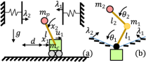
Figure 1: (a): cartpole with softwalls. (b): acrobot with soft joints.

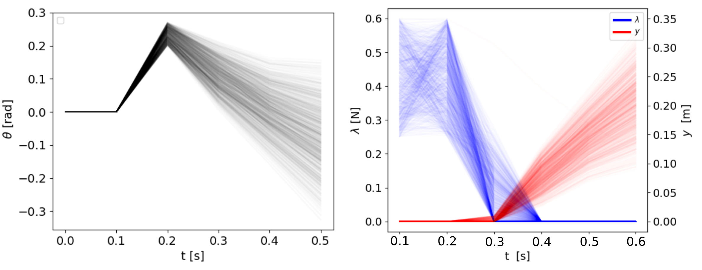
Figure 2: Uncertainty propagation for cartpole system. Here only uncertainty arises from stiffness parameters $k_{1},k_{2}$.

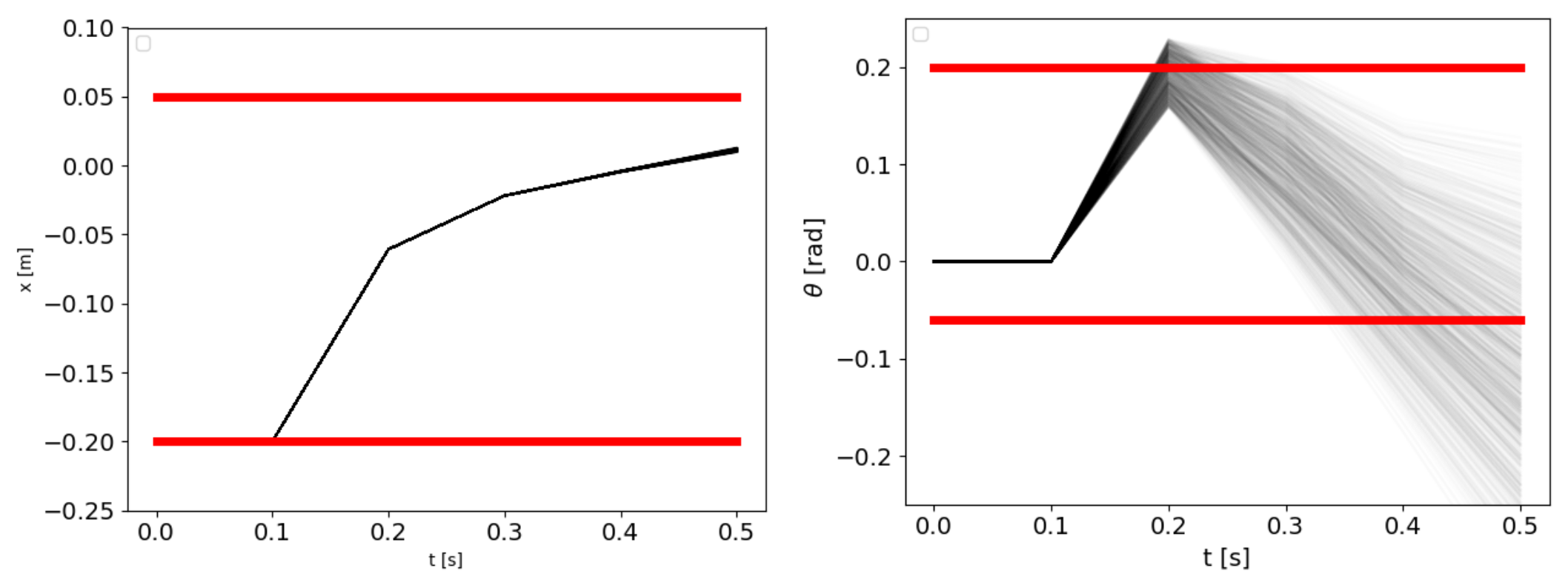
Figure 3: Simulated trajectories for cartpole system using ERM-based controller. $\Delta=0.2$ and $\Delta_{\text{test}}=0.083$. Red lines show boundaries specified in chance constraints.

We show uncertainty evolution for SDLCS. We demonstrate this for a cartpole system with softwalls (see [14] for more details). Here we consider both $k_{1}$ and $k_{2}$ follows uniform distributions where upper bound of uniform distribution for $k_{1}$ and $k_{2}$ is 14, 12, respectively, and the lower bound is 5 for both $k_{1}$ and $k_{2}$. In this experiment, we do not run any controller: we simply propagate SDLCS given uncertain parameters in order to show how the SDLCS behaves.

Fig. 2 shows the evolution of uncertainty for the aforementioned system. At $t=0$ s, there is no uncertainty for state $\theta_{t=0}$. However, because we provide uncertainty with $k_{1}$ and $k_{2}$, $\lambda_{t=0.1}$ has uncertainty. This is again because given realization of uncertain parameters, complementarity constraints give a realization of $\lambda$ and $y$, resulting in uncertainty in $\lambda$ and $y$. This stochastic $\lambda_{t=0.1}$ brings uncertainty in $\theta_{t=0.1}$ based on (1). As shown in Fig. 2, both state and complementarity variables are stochastic. This can not be captured in approximations like Expected Residual Minimization (ERM) [15].

V-B Cartpole with Softwalls

We demonstrate our open- and closed-loop controllers for cartpole with softwalls system. $x$ is the cart position and $\theta$ is the pole angle. $u_{1}$ is the control and $\lambda_{1},\lambda_{2}$ are the reaction forces at from the wall 1, 2, respectively. We have the following deterministic physical parameters. $g=9.81$ is the gravitational acceleration, $m_{p}=0.1,m_{c}=1.0$ are the mass of the pole, cart, respectively. $l=0.5$ is the length of the pole and $d=0.15$ is the distance from the origin of the coordinate to the walls. We assume that the uncertainty arises from the ${k_{1}},{k_{2}}$ and use the same distribution in Sec V-A. We set $dt=0.1$ for the explicit Euler integration and $T=6$.

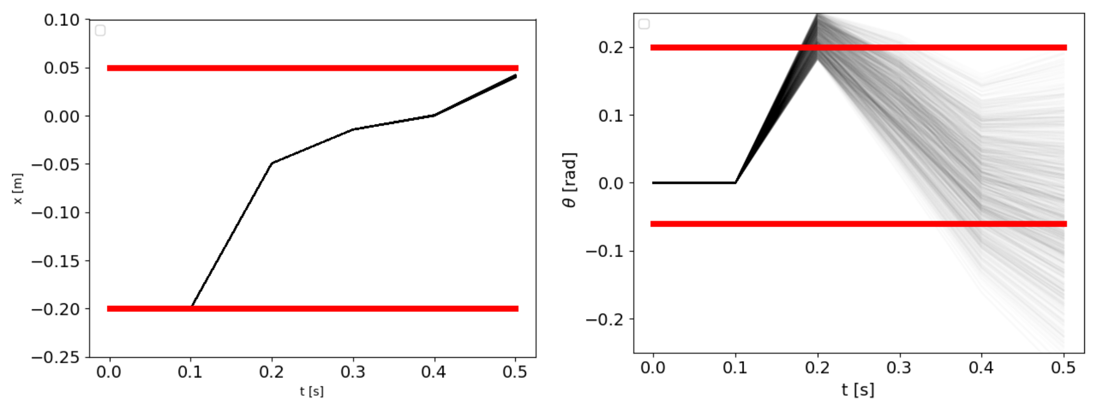
Figure 4: Simulated trajectories for cartpole system using our open-loop controller. $\Delta=0.2$ and $\Delta_{\text{test}}=0.190$ where $\Delta$ is input of optimization and $\Delta_{\text{test}}$ is the empirically obtained success rate from MC simulation. Red lines show boundaries specified in chance constraints.

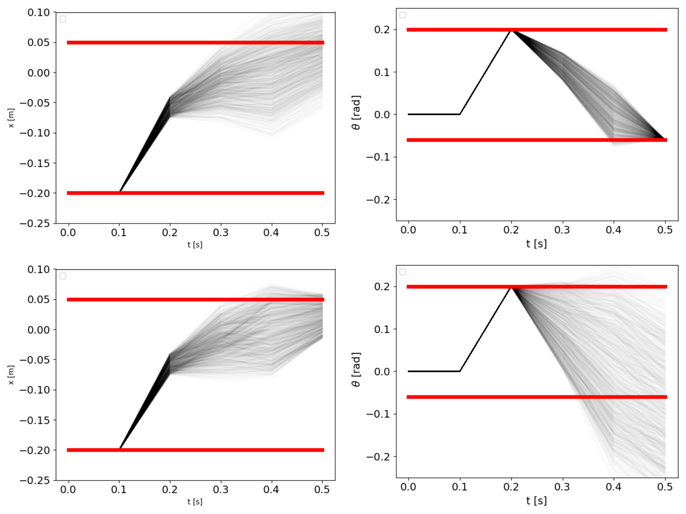
Figure 5: Simulated trajectories for cartpole system using our closed-loop controller. Top: $\Delta=0.6$ and $\Delta_{\text{test}}=0.510$, bottom: $\Delta=0.2$ and $\Delta_{\text{test}}=0.188$, where $\Delta$ is input of optimization and $\Delta_{\text{test}}$ is the empirically obtained success rate from MC simulation. Red lines show boundaries specified in chance constraints.

The results using ERM and our controller for the open-loop trajectory are shown in Fig. 3, Fig. 4. We observed that the proposed open-loop controller shows the better satisfaction of chance constraints compared to the ERM-based method. This is because our method explicitly considers propagation of uncertainty for SDLCS while the ERM-based method is unable to consider. Also, we observe that the gap between the commanded $\Delta$ used in our optimization and $\Delta_{\text{test}}$ obtained from MC simulation over testing dataset is smaller the gap between the commanded $\Delta$ used in ERM method and $\Delta_{\text{test}}$ obtained from MC simulation over testing dataset. Again this is because our method could capture the evolution of uncertainty for SDLCS. However, even our open-loop controller does not show the much better performance than the ERM. To show the higher $\Delta_{\text{test}}$, we need to input the higher $\Delta$ as an input of optimization. It is quite difficult especially for long-horizon planning problems since uncertainty keeps evolving, which can be observed from both Fig. 3 and Fig. 4.

Next, we discuss the difference among our proposed contact-aware closed-loop, the non-contact-aware (i.e., $L_{k}=0,\forall k$ in (5b)) closed loop, and the open-loop controllers. We observed that in Table I, (9) for open-loop controller with high $\Delta$ was unable to find feasible solutions but (9) for closed-loop controller could find feasible solutions. Since the closed-loop controller can change feedback gains to satisfy chance constraints, it could find feasible solutions with high $\Delta$. Also, Table I shows that the contact-aware closed-loop controller could find the feasible solution with high $\Delta=0.8,0.7$ but the non-contact-aware controller (i.e., $L_{k}=0,\forall k$ in (5b)) could not. For SDLCS, introducing feedback to both states and forces is important to realize the robust motion. The MC simulation results using our contact-aware closed-loop controller are shown in Fig. 5. In contrast to Fig. 3 and Fig. 4, the closed-loop controller could bound the distribution of the states because it controls covariance.

We discuss computational results. Firstly, we observe that our important-particle method converges and the gap between $\Delta_{\text{train}}$ and $\Delta_{\text{test}}$ is small once it finishes its third time iteration. It means that our important-particle method could successfully find feasible trajectories with relative small number of particles. Secondly, in Table II the important-particle method shows the higher $\Delta_{\text{train}}$ as the number of particles used in optimization increases. The proposed important-particle method shows better convergence (in total 208 s to have $\Delta_{\text{train}}\geq 0.49$) than the naive method (620 s with 50 particles to have $\Delta_{\text{test}}\geq 0.49$) since our important-particle method keeps choosing the worst-case particles which break chance constraints.

TABLE I: Comparison of feasibility for cartpole system among open-, non-contact-aware closed, and contact-aware-closed controllers with different $\Delta$. $\circ$ and $\times$ show if optimization finds a feasible solution or not, respectively.

$\Delta$	$0.8$	$0.7$	$0.6$	$0.4$	$0.2$
Open-loop	$\times$	$\times$	$\times$	$\circ$	$\circ$
Non-contact-aware closed-loop	$\times$	$\times$	$\circ$	$\circ$	$\circ$
Contact-aware closed-loop	$\circ$	$\circ$	$\circ$	$\circ$	$\circ$

TABLE II: Comparison of safe probability and runtime for cartpole system between important-particle method (top) with $\gamma=10,\eta=10$ and naive method (bottom) with $\Delta=0.6$ for designing the closed-loop controller. $T$ represents runtime for each iteration and $n_{p}$ is the number of particles.

iter	$1$	$2$	$3$
$\Delta_{\text{train}}$	0.2708	0.09	0.592
$\Delta_{\text{test}}$	N/A	N/A	0.588
T [s]	25	35	148
$n_{p}$	10	20	30

Case	1	2	3	4
$\Delta_{\text{test}}$	0.277	0.376	0.451	0.499
T [s]	25	26	55	620
$n_{p}$	10	20	30	50

V-C Acrobot with Soft Joints

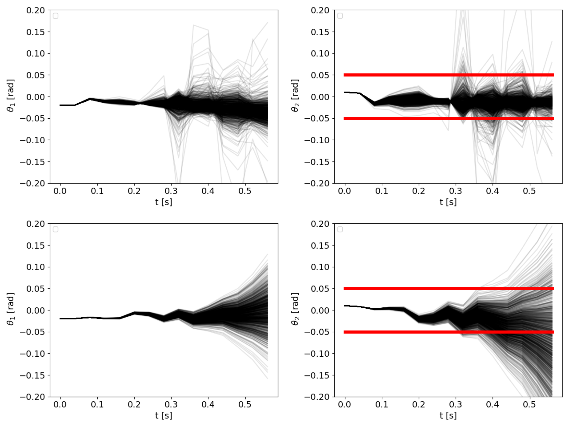
Figure 6: Simulated trajectories for acrobot using our open- and closed-loop controllers. Top: closed-loop controller with $\Delta=0.8$ and $\Delta_{\text{test}}=0.771$, bottom: open-loop controller with $\Delta=0.4$ and $\Delta_{\text{test}}=0.366$. Red lines show boundaries specified in chance constraints. The reader should note that open-loop controller solution was infeasible for $\Delta=0.8$, and thus we show results for $\Delta=0.4$.

TABLE III: Comparison of safe probability and runtime for acrobot system between important-particle method (top) with $\gamma=4,\eta=4$ and naive method (bottom) with $\Delta=0.8$. $T$ represents runtime for each iteration and $n_{p}$ is the number of particles.

iter	$1$	$2$	$3$	$4$	$5$	$6$	$7$
$\Delta_{\text{train}}$	0.426	0.485	0.562	0.625	0.363	0.593	0.763
$\Delta_{\text{test}}$	N/A	N/A	N/A	N/A	N/A	N/A	0.771
$T$ [s]	31	97	557	887	698	2450	779
$n_{p}$	4	8	12	16	20	24	28

Case	1	2	3	4	5	6	7
$\Delta_{\text{test}}$	0.009	0.103	0.159	0.541	0.670	0.553	0.539
$T$ [s]	31	15	229	260	944	3993	901
$n_{p}$	4	8	12	16	20	24	28

We also demonstrate our controller for acrobot with soft joints system (see [14] for more details). $\theta_{1}$ is the first joint angle and $\theta_{2}$ is the second joint angle. $u_{1}$ is the control at the second joint and $\lambda_{1},\lambda_{2}$ are the reaction forces at from the wall 1, 2, respectively. We have the following deterministic physical parameters.$g=9.81$ is the gravitational acceleration, $m_{1}=0.5,m_{2}=1.0$ are the mass of the pole, cart, respectively. $l_{1}=0.5$ is the length of the rod from the first to the second joint. $d=0.2$ is the angle limit of $\theta_{1}$. We consider the stochastic physical parameters $k$ and $l_{2}$ where $k$ is the stiffness of the walls and $l_{2}$ is the length of the second rod. We assume that $k$ follows uniform distribution where the upper bound and the lower bound of the distribution is 1.6 and 0.6, respectively. We assume that $l_{2}$ follows a truncated Gaussian distribution where we set the mean to 1.0, variance to 0.01, the upper bound of the interval is 1.3, and the lower bound of the interval is 0.7, respectively. We set $dt=0.04$ for the explicit Euler integration and $T=15$.

The open- and closed-loop trajectories are shown in Fig. 6. We observed that both controller could satisfy chance constraints over the testing dataset and the closed-loop controller shows the better performance. Table III shows that the important-particle method shows the higher $\Delta_{\text{test}}=0.771$ than the naive method with the same number of particles used in optimization.

VI Discussion

Stochastic complementarity systems are not well understood in literature. This paper presents a study of SDLCS to perform covariance steering using particles. Under the assumption of uniqueness of trajectory ($\bar{F}$ is P-matrix) for complementarity systems, the proposed method is able to compute covariance controller for SDLCS. We presented an important-particle method to alleviate computational complexity of the resulting optimization problem. It is shown that our work could design open- and closed-loop controllers with chance constraints by appropriately considering the evolution of uncertainty for SDLCS.

In the future, we would like to study more general manipulation systems by relaxing the assumption on uniqueness of trajectory for SDLCS. Another limitation of this work is that the computation is still demanding. Thus, we would like to employ distributed optimization techniques such as ADMM [29].

References

- [1] Y. Shirai, D. K. Jha, A. Raghunathan, and D. Romeres, “Chance-constrained optimization in contact-rich systems for robust manipulation,” arXiv preprint arXiv:2203.02616, 2022.
- [2] M. Ono and B. C. Williams, “Iterative risk allocation: A new approach to robust model predictive control with a joint chance constraint,” in 2008 47th IEEE Conference on Decision and Control, 2008, pp. 3427–3432.
- [3] L. Blackmore and M. Ono, “Convex chance constrained predictive control without sampling,” in AIAA guidance, navigation, and control conference, 2009, p. 5876.
- [4] L. Blackmore, M. Ono, A. Bektassov, and B. C. Williams, “A probabilistic particle-control approximation of chance-constrained stochastic predictive control,” IEEE Transactions on Robotics, vol. 26, no. 3, pp. 502–517, 2010.
- [5] T. Lew, R. Bonalli, and M. Pavone, “Chance-constrained sequential convex programming for robust trajectory optimization,” in 2020 European Control Conference (ECC), 2020, pp. 1871–1878.
- [6] Y. K. Nakka and S.-J. Chung, “Trajectory optimization of chance-constrained nonlinear stochastic systems for motion planning and control,” arXiv preprint arXiv:2106.02801, 2021.
- [7] Y. Shirai, X. Lin, Y. Tanaka, A. Mehta, and D. Hong, “Risk-aware motion planning for a limbed robot with stochastic gripping forces using nonlinear programming,” IEEE Robotics and Automation Letters, vol. 5, no. 4, pp. 4994–5001, 2020.
- [8] Y. Shirai, D. K. Jha, A. U. Raghunathan, and D. Romeres, “Robust pivoting: Exploiting frictional stability using bilevel optimization,” in Proc. 2022 IEEE Int. Conf. Robo. Auto., 2022, pp. 992–998.
- [9] Y. Shirai, D. K. Jha, and A. U. Raghunathan, “Robust pivoting manipulation using contact implicit bilevel optimization,” 2023. [Online]. Available: https://arxiv.org/abs/2303.08965
- [10] M. Posa, C. Cantu, and R. Tedrake, “A direct method for trajectory optimization of rigid bodies through contact,” Int. J. Rob. Res., vol. 33, no. 1, pp. 69–81, 2014.
- [11] A. U. Raghunathan, D. K. Jha, and D. Romeres, “Pyrobocop: Python-based robotic control optimization package for manipulation,” in Proc. 2022 IEEE Int. Conf. Robo. Auto., 2022, pp. 985–991.
- [12] J. Carius, R. Ranftl, V. Koltun, and M. Hutter, “Trajectory optimization for legged robots with slipping motions,” IEEE Robotics and Automation Letters, vol. 4, no. 3, pp. 3013–3020, 2019.
- [13] Y. Shirai, X. Lin, A. Schperberg, Y. Tanaka, H. Kato, V. Vichathorn, and D. Hong, “Simultaneous contact-rich grasping and locomotion via distributed optimization enabling free-climbing for multi-limbed robots,” in Proc. 2022 IEEE/RSJ Int. Conf. Intell. Rob. Syst., 2022, pp. 13 563–13 570.
- [14] A. Aydinoglu, V. M. Preciado, and M. Posa, “Contact-aware controller design for complementarity systems,” in 2020 IEEE International Conference on Robotics and Automation (ICRA), 2020, pp. 1525–1531.
- [15] L. Drnach and Y. Zhao, “Robust trajectory optimization over uncertain terrain with stochastic complementarity,” IEEE Robot. Autom. Lett., vol. 6, no. 2, pp. 1168–1175, 2021.
- [16] S. Thrun, “Probabilistic robotics,” Communications of the ACM, vol. 45, no. 3, pp. 52–57, 2002.
- [17] S. J. Julier and J. K. Uhlmann, “Unscented filtering and nonlinear estimation,” Proceedings of the IEEE, vol. 92, no. 3, pp. 401–422, 2004.
- [18] A. Wang, X. Huang, A. Jasour, and B. Williams, “Fast risk assessment for autonomous vehicles using learned models of agent futures,” arXiv preprint arXiv:2005.13458, 2020.
- [19] A. Jasour, A. Wang, and B. C. Williams, “Moment-based exact uncertainty propagation through nonlinear stochastic autonomous systems,” arXiv preprint arXiv:2101.12490, 2021.
- [20] A. Hotz and R. E. Skelton, “Covariance control theory,” International Journal of Control, vol. 46, no. 1, pp. 13–32, 1987.
- [21] K. Okamoto and P. Tsiotras, “Optimal stochastic vehicle path planning using covariance steering,” IEEE Robotics and Automation Letters, vol. 4, no. 3, pp. 2276–2281, 2019.
- [22] J. Ridderhof, K. Okamoto, and P. Tsiotras, “Nonlinear uncertainty control with iterative covariance steering,” in 2019 IEEE 58th Conference on Decision and Control (CDC). IEEE, 2019, pp. 3484–3490.
- [23] J. Luedtke and S. Ahmed, “A sample approximation approach for optimization with probabilistic constraints,” SIAM Journal on Optimization, vol. 19, no. 2, pp. 674–699, 2008. [Online]. Available: https://doi.org/10.1137/070702928
- [24] B. K. Pagnoncelli, S. Ahmed, and A. Shapiro, “Sample average approximation method for chance constrained programming: theory and applications,” Journal of optimization theory and applications, vol. 142, no. 2, pp. 399–416, 2009.
- [25] M. A. Sehr and R. R. Bitmead, “Particle model predictive control: Tractable stochastic nonlinear output-feedback mpc,” IFAC-PapersOnLine, vol. 50, no. 1, pp. 15 361–15 366, 2017.
- [26] R. Cottle, J. Pang, and R. Stone, The Linear Complementarity Problem, ser. Classics in Applied Mathematics. Society for Industrial and Applied Mathematics, 2009.
- [27] N. Jorge and J. W. Stephen, “Numerical optimization,” 2006.
- [28] A. Wächter and L. Biegler, “On the implementation of an interior-point filter line-search algorithm for large-scale nonlinear programming,” Mathematical Programming, vol. 106, no. 1, pp. 25–57, May 2006.
- [29] S. Boyd, N. Parikh, E. Chu, B. Peleato, J. Eckstein et al., “Distributed optimization and statistical learning via the alternating direction method of multipliers,” Foundations and Trends® in Machine learning, vol. 3, no. 1, pp. 1–122, 2011.