Information transmission in monopolistic
credence goods markets

Abstract

We study a general credence goods model with $N$ problem types and $N$ treatments. Communication between the expert seller and the client is modeled as cheap talk. We find that the expert’s equilibrium payoffs admit a geometric characterization, described by the quasiconcave envelope of his belief-based profits function under discriminatory pricing. We establish the existence of client-worst equilibria, apply the geometric characterization to previous research on credence goods, and provide a necessary and sufficient condition for when communication benefits the expert. For the binary case, we solve for all equilibria and characterize client’s possible welfare among all equilibria.

Keywords: Credence Goods, Cheap Talk, Quasiconcave Envelope, Belief-based Approach

JEL Code: D82, D83, L12

1 Introduction

A credence good is a product or service whose qualities or appropriateness are hard to evaluate for clients even after consumption. Typical examples of credence goods include medical services, automobile repairs and financial advice. Patients who undergo an expensive medical treatment may find it difficult to evaluate its worth after they have been cured, car owners may be skeptical about the necessity of replacing an entire engine for car repairs, and investors with limited financial literacy are not able to determine the appropriateness of a financial product even after the returns have been realized. In contrast, expert sellers often have superior knowledge about the appropriateness of credence goods, and may exploit this information advantage for their own benefits.

A common assumption in the credence goods literature is that clients do not have full choice rights; that is, a client can only accept or reject the expert’s recommended option, or may even commit ex ante to accepting the expert’s recommendation when they visit the expert. While this assumption applies to many important credence goods markets, such as medical services, it does not apply to many other credence goods markets such as car repair, financial advice, and taxi rides. For example, an investor may choose a more conservative asset allocation after being advised to take on higher risks for more potential rewards, and a passenger can often insist on choosing their preferred route despite the taxi driver’s suggestion of another route. To address this discrepancy, this paper examines a credence goods model in which clients have the full choice right, allowing them to self-select their most desired options after receiving expert advice. Accordingly, an expert’s recommendation is modeled as a cheap-talk message and does not restrict a client’s choice set.

In this paper, we consider a general $N$-by-$N$ model of credence goods, in which the client’s problem can be one of $N$ possible types and the expert offers $N$ treatment options for the client to choose from. The expert sets prices before the client’s visit. After privately observing the client’s problem type, the expert sends a cheap-talk message to the client. Then the client self-selects her most desired option. We characterize the expert’s payoffs in subgames following the price setting stage using the quasiconcave envelope approach introduced by Lipnowski and Ravid (2020), and further show that the expert’s equilibrium payoffs of the whole game are the quasiconcave envelope of the belief-based profits function under discriminatory pricing. This geometric characterization allows for a novel interpretation: one can compute the expert’s equilibrium payoffs as if the client and the expert are playing an alternative game in which the expert sets prices after meeting and advising the client. Somewhat surprisingly, the expert’s equilibrium payoffs do not increase even if he is allowed to charge discriminatory prices targeted at clients with different posteriors. Based on the alternative game, we further show that our characterization of the expert’s equilibrium payoffs also applies to previous research on credence goods, in which the client either accepts or rejects the recommended treatment. This observation strengthens the connection between our paper and the credence goods literature.

1.1 Literature

This paper is related to the literature of credence goods. The concept of credence goods was first introduced by Darby and Karni (1973), and subsequent works have examined the incentives for the expert to defraud clients. Due to the significant information advantages that experts possess, the market for credence goods may break down if experts’ behaviors are not constrained. To address this issue, existing works have either assumed that (i) an expert is liable to fix a client’s problem (Pitchik and Schotter, 1987; Wolinsky, 1993; Fong, 2005; Liu, 2011; Fong, Hu, Liu, and Meng, 2020) or that (ii) the type of expert-provided good or service is observable and verifiable by clients (Emons, 1997; Dulleck and Kerschbamer, 2009; Fong, Liu, and Wright, 2014; Bester and Dahm, 2017). In a comprehensive review by Dulleck and Kerschbamer (2006), they refer to these two assumptions as the “liability assumption” and the “verifiability assumption” respectively. In this paper, we impose the verifiability assumption. Furthermore, as mentioned in the introduction, it is assumed that clients are free to choose their preferred option after receiving the expert’s recommendation. In previous research on credence goods, the expert’s recommendation serves not only to provide information but also to restrict the client’s choice set. Specifically, some previous studies assume that clients must commit to accepting the recommended treatment before consulting the expert (e.g., Emons, 1997; Bester and Dahm, 2017), which is known as the “commitment assumption” in Dulleck and Kerschbamer (2006). Other studies assume that clients can only accept or reject the treatment recommended by the expert (e.g., Pitchik and Schotter, 1987; Wolinsky, 1993; Fong, 2005; Dulleck and Kerschbamer, 2009; Liu, 2011; Fong, Liu, and Wright, 2014; Fong et al., 2020).

Our paper is closest to Fong, Liu, and Wright (2014) who study a specific case of our setup with two treatments and two problem types. In Fong, Liu, and Wright (2014), the expert recommends a treatment and then the client decides whether to accept or reject the recommended treatment. However, in our model, the expert sends a cheap-talk message and then the client self-selects their most desired option. Despite the differences in model setups, our characterization of the expert’s equilibrium payoffs can also be applied to the setting of Fong, Liu, and Wright (2014), which will be discussed in Section 3.

Second, our paper is also related to the literature on cheap talk, particularly studies that focus on cheap talk models with state-independent sender preferences (Chakraborty and Harbaugh, 2010; Lipnowski and Ravid, 2020; Diehl and Kuzmics, 2021; Corrao and Dai, 2023). In this paper, we model the expert’s recommendation as a cheap-talk message à la Crawford and Sobel (1982). Furthermore, the expert has state-independent preferences since the expert’s payoffs, after prices are set, are determined solely by the client’s choice. For this class of cheap talk models, Lipnowski and Ravid (2020) develop the quasiconcave envelope approach to characterize the expert’s equilibrium payoffs in a general setting. In our model, the subgames following the expert’s price-setting stage are specialized cases of Lipnowski and Ravid (2020). However, with the additional price-setting stage before the communication, expert’s equilibrium payoffs become the upper envelope of those quasiconcave envelopes and are hard to calculate. One of our main contributions is to further characterize the expert’s equilibrium payoffs as the quasiconcave envelope of his belief-based profits function (1). Furthermore, by applying the geometric characterization to previous works on credence goods, we also demonstrate that the quasiconcave envelope approach for cheap talk games can be used for other games where talk is not cheap.

Finally, our paper contributes to the growing field of research at the interplay of information transmission (or information acquisition) and optimal pricing. A recurring theme in this literature is the strategic intersection between the seller’s (buyer’s) information revelation (acquisition) and the seller’s price setting. Lewis and Sappington (1994) consider a scenario in which a seller both sets prices and designs the information structure of the buyers’ valuations for the product. Roesler and Szentes (2017) examine a bilateral trade model in which the buyer is free to choose any signal structure concerning her valuation. They find that there exists a buyer-optimal signal structure which results in efficient trade and a unit-elastic demand. In a subsequent work, Ravid, Roesler, and Szentes (2022) investigate a similar model in which learning is costly for the buyer and the buyer’s signal structure is not observed by the seller. They find that as the learning cost approaches zero, the equilibria converge to the worst free-learning equilibrium. Chen and Zhang (2020) study a bilateral trade model in which the seller utilizes both Bayesian persuasion and pricing to signal the product quality. They identify a unique separating equilibrium that satisfies the intuitive criterion. In our paper, the setup involves multiple products instead of a single product. The expert (i.e., seller) employs a combination of strategic pricing and cheap-talk communication to maximize the expected profits. We find that the expert’s equilibrium payoffs admit a geometric characterization and, somewhat surprisingly, the expert’s equilibrium payoffs do not increase even if he is allowed to charge differentiated prices targeted at buyers with different posteriors.

The rest of the paper is as follows. Section 2 presents the $N$-by-$N$ model and the geometric characterization of the expert’s equilibrium payoffs. Section 3 applies the geometric characterization to previous credence goods research. Section 4 characterizes all the equilibria in the binary case. Section 5 gives a necessary and sufficient condition for when communication benefits the expert. Section 6 concludes. Omitted proofs are relegated to Appendix.

2 Model

2.1 Environment

There are two players: Client (she) and Expert (he). Both players are risk-neutral. Client has a problem but is uncertain about the problem type $t$, which is drawn from $T\equiv\{\,{t_{1}},\dots,{t_{N}}\,\}$ according to the distribution $\mu^{0}$. If a problem of type $t_{i}$ remains unresolved, Client will suffer a disutility of $l_{i}$ for $i\in\{\,{1},\dots,{N}\,\}$. Client consults Expert who privately observes the problem type. Expert provides $N$ different treatments, denoted by $\{a_{j}\}_{j=1}^{N}$, that vary in their efficacy. Specifically, treatment $a_{j}$ is effective in fully resolving a problem of type $t_{i}$ for all $i\leq j$, but cannot resolve a problem of type $t_{i^{\prime}}$ with $i^{\prime}>j$; treatment $a_{N}$ is a panacea that fully resolves all problems. Denote by $c_{j}$ the cost of treatment $a_{j}$ for Expert. Expert’s treatments are credence goods: Once a problem has been resolved through the use of treatment $a_{j}$ with $j\geq 2$, Client remains uncertain about whether an alternative treatment, such as $a_{i}$ with $i<j$, could have resolved her problem as well.

Assume that Expert incurs no cost when diagnosing the problem type. Following the diagnosis, Expert sends a cheap-talk message to Client, which is interpreted as a treatment recommendation. Upon receiving the message, Client chooses $a\in A\equiv\{a_{0},a_{1},\dots,a_{N}\}$, where $a_{0}$ denotes the decision not to purchase any treatment. It is assumed that Client is able to observe and verify the type of performed treatment (i.e., the verifiability assumption).

Timing of the game is as follows:

1. Expert posts a price list $p=(p_{1},\dots,p_{N})\in\mathbb{R}_{+}^{N}$, where $p_{j}$ is the price for treatment $a_{j}$ for $j\in\set{1,\dots,N}$.

2. Client visits and Expert privately observes the problem type $t$, which is drawn according to the distribution $\mu^{0}\in\Delta(T)$ with $T=\set{t_{1},\dots,t_{N}}$.

3. Expert sends a message $m$, from the message set $M$, to Client.

4. After receiving $m$, Client chooses $a\in A=\set{a_{0},a_{1},\dots,a_{N}}$.

5. Client and Expert obtain payoffs $u^{C}(t,a,p)$ and $u^{E}(a,p)$ respectively. When $a=a_{0}$, their payoffs are $u^{C}(t_{i},a_{0},p)=-l_{i}$ and $u^{E}(a_{0},p)=0$ for all $i\in\{\,{1},\dots,{N}\,\}$ and $p\in\mathbb{R}_{+}^{N}$; when $a\neq a_{0}$,

   $$u^{C}(t_{i},a_{j},p)=-p_{j}-\mathbf{1}(j<i)\cdot l_{i},\quad u^{E}(a_{j},p)=p_{j}-c_{j}$$ (1)

   where $\mathbf{1}(j<i)$ is the indicator function that takes the value of $1$ when $j<i$ and $0$ otherwise.

Throughout this paper, we impose the following assumptions. First, the message set $M$ is assumed to be finite and of a sufficiently large size. Second, the cost of a treatment is increasing in its index: $c_{j}>c_{i}$ whenever $j>i$. This assumption is realistic since a treatment of a higher index is always more likely to resolve the problem. Third, all treatments are efficient in that $s_{j}\equiv l_{j}-c_{j}>0$ for $j\in\{\,{1},\dots,{N}\,\}$. We do not require that the loss caused by a problem is increasing in its type index (i.e., $l_{j}>l_{i}$ whenever $j>i$). The implication is that a problem of a higher type is more difficult to resolve, but may not cause a higher loss to Client if left unresolved.

2.2 Solution concept

Our solution concept is the Expert-optimal perfect Bayesian equilibrium (henceforth, equilibrium). To elaborate, we first define the notion of $p$-equilibrium for the subgame following Expert posting some price list $p$.

Definition 1 ($p$-equilibrium).

Given a price list $p\in\mathbb{R}_{+}^{N}$, a $p$-equilibrium consists three maps: Expert’s signalling strategy $\sigma:T\to\Delta(M)$; Client’s strategy $\rho:M\to\Delta(A)$; and Client’s belief updating $\beta:M\to\Delta T$; such that

1. Given Expert’s signalling strategy $\sigma$, Client’s posterior belief after receiving $m$ is obtained from the prior $\mu^{0}$ using Bayes’s rule whenever possible:

   $$\beta(t_{i}\mid m)=\frac{\mu^{0}(t_{i})\sigma(m\mid t_{i})}{\sum_{k=1}^{N}\mu^{0}(t_{k})\sigma(m\mid t_{k})}$$

   for $t_{i}\in T$. If $\sigma(m|t_{i})=0$ for all $t_{i}\in T$, then Client puts probability one on some problem type of index $i\in\operatorname{\mathsf{arg}}\min_{i}l_{i}-c_{i}$.

2. Given the belief updating $\beta$, Client’s strategy $\rho(\cdot\mid m)$ after receiving message $m$ is supported on

   $$\operatorname{\mathsf{arg}}\operatorname{\mathsf{max}}_{a\in A}\sum_{t\in T}u^{C}(a,t,p)\beta(t\mid m)$$

   for $m\in M$.

3. Given Client’s strategy $\rho$, Expert’s signalling strategy $\sigma(\cdot\mid t)$ is supported on

   $$\operatorname{\mathsf{arg}}\operatorname{\mathsf{max}}_{m\in M}\sum_{a\in A}\rho(a\mid m)u^{E}(a,p)$$

   for $t\in T$.

A $p$-equilibrium is called an Expert-optimal $p$-equilibrium if it yields the highest payoff for Expert among all $p$-equilibria under the price list $p$. When there exist multiple $p$-equilibria, assume (one of) the Expert-optimal $p$-equilibria will be played. Specifically, given some price list $\tilde{p}$, Expert’s expected payoff in any Expert-optimal $\tilde{p}$-equilibrium is:

$$\begin{split}&U^{E}(\tilde{p})=\sum_{i=1}^{N}\mu^{0}(t_{i})\left(\sum_{a\in A}\rho(a\mid{m_{i}})u^{E}(a,\tilde{p})\right)\end{split}$$ (2)

where $(\beta,\rho,\sigma)$ is some Expert-optimal $\tilde{p}$-equilibrium and $m_{i}\in\operatorname{\mathsf{supp}}\sigma(\cdot\mid t_{i})$. We refer to $U^{E}(\tilde{p})$ as Expert’s maximal $\tilde{p}$-equilibrium payoff, i.e., his ex ante payoff in an Expert-optimal $\tilde{p}$-equilibrium. Note that one can use any Expert-optimal $\tilde{p}$-equilibrium to compute $U^{E}(\tilde{p})$ because, given the same price list $\tilde{p}$, all Expert-optimal $\tilde{p}$-equilibria yield the same payoff for Expert. Also, in Equation 2, $m_{i}$ can be any message from the support of $\sigma(\cdot\mid t_{i})$. The reason is that in any $\tilde{p}$-equilibrium, Expert is indifferent among sending any message from the support of $\sigma(\cdot\mid t_{i})$ given the problem type $t_{i}$.

Before Client visits, Expert chooses some price list to maximize $U^{E}(p)$:

$$p^{*}\in\operatorname{\mathsf{arg}}\operatorname{\mathsf{max}}\operatorname{\mathsf{max}}_{p\in\mathbb{R}^{N}_{+}}U^{E}(p).$$ (3)

To sum up, an equilibrium of our model is described by a price list $p^{*}$ that solves (3) and the Expert-optimal $p$-equilibria for all $p\in\mathbb{R}^{N}_{+}$. While we consider only pure pricing strategies in problem (3), this is not a restriction of generality. The reason is that an equilibrium in which Expert takes a mixed price-setting strategy exists if and only if there are multiple price lists that yield the highest payoffs for Expert; when such an equilibrium with a mixed pricing strategy exists, it can be expressed as a convex combination of the corresponding equilibria with pure pricing strategies that also yield the highest payoff for Expert.

Roadmap

Methodologically, we first use the quasiconcave envelope approach invented by Lipnowski and Ravid (2020) to geometrically describe Expert’s maximal $p$-equilibrium payoffs. Based on that result, we further give a geometric characterization of Expert’s equilibrium payoffs. This characterization also implies the existence of some specific kind of equilibria in which Client does not benefit from Expert’s services.

2.3 Expert’s $p$-equilibrium payoffs

We calculate Expert’s $p$-equilibrium payoffs using the belief-based approach, which focuses on the equilibrium outcomes and abstracts away Expert’s signalling strategy $\sigma$ and Client’s strategy $\rho$. Let $\set{\mu^{1},\dots,\mu^{K}}$ be a set of beliefs where $\mu^{k}\in\Delta(T)$ for all $k\in\{\,{1},\dots,{K}\,\}$, and we call this set a splitting of $\mu$ if there exist $K$ non-negative numbers, $\set{{\lambda_{1}},\dots,{\lambda_{K}}}$ with $\sum_{k=1}^{K}\lambda_{k}=1$, such that $\sum_{k=1}^{K}\lambda_{k}\mu^{k}=\mu$. We use a splitting of the prior $\mu^{0}$ to describe Client’s possible posteriors in an outcome of our model. Specifically, the pair $(\{\,{\mu^{1}},\dots,{\mu^{K}}\,\},v)$ is called an (Expert-optimal) $p$-equilibrium outcome if there exists some (Expert-optimal) $p$-equilibrium in which (i) the ex ante distribution of Client’s posteriors has $\{\,{\mu^{1}},\dots,{\mu^{K}}\,\}$ as its support and (ii) Expert’s $p$-equilibrium payoff is $v\in\mathbb{R}$. An equilibrium outcome is a triple $(\tilde{p},\{\,{\mu^{1}},\dots,{\mu^{K}}\,\},\tilde{v})$ where the price list $\tilde{p}$ solves problem (3) and $(\{\,{\mu^{1}},\dots,{\mu^{K}}\,\},\tilde{v})$ is a $\tilde{p}$-equilibrium outcome.

Let $\bar{a}(\mu,p)$ be the set of Client’s (possibly mixed) optimal choices given belief $\mu$ and price list $p$. Correspondingly, the set of Expert’s possible payoffs is:

$$V(\mu;p)\equiv u^{E}(\bar{a}(\mu,p),p).$$

Here $V(\,\cdot\,;p):\Delta T\rightrightarrows\mathbb{R}$ is a correspondence parameterized by $p\in\mathbb{R}_{+}^{N}$. Let $\bar{v}(\mu\,;p)\equiv\operatorname{\mathsf{max}}V(\mu\,;p)$. For any $p\in\mathbb{R}^{N}_{+}$, it follows from Berge’s theorem that $V(\,\cdot\,;p)$ is a Kakutani correspondence on $\Delta(T)$ and the function $\bar{v}(\,\cdot\,;p)$ is upper semicontinuous on $\Delta(T)$. Fixing any $p\in\mathbb{R}_{+}^{N}$, Expert’s maximal $p$-equilibrium payoff $U^{E}(p)$, as defined in (2), is equal to the value of the following maximization problem:

$$\begin{split}U^{E}(p)=&\operatorname{\mathsf{max}}_{\{\mu^{1},\dots,\mu^{K}\}}{v}\\ \text{subject to }&\text{(i) $v\in V(\mu^{k};p)$ for all }k\in\{\,{1},\dots,{K}\,\};\\ &\text{(ii) $\{\mu^{1}$, \ldots, $\mu^{K}\}$ is a splitting of $\mu^{0}$}.\end{split} \mathcal{M}$$ ()

Condition (i) combines restrictions (b) and (c) of 1 and condition (ii) captures restriction (a) of 1. In a seminal paper, Lipnowski and Ravid (2020) show that the value function for problem ($\mathcal{M}$) allows for a geometric representation. Specifically, call $\operatorname{\mathsf{qcav}}\bar{v}(\,\cdot\,;p)$ the quasiconcave envelope of $\bar{v}(\,\cdot\,;p)$ if, fixing $p$, function $\operatorname{\mathsf{qcav}}\bar{v}(\,\cdot\,;p)$ is the pointwise lowest quasiconcave function that is everywhere above $\bar{v}(\,\cdot\,;p)$. Expert’s maximal $p$-equilibrium payoff as described by ($\mathcal{M}$) is exactly $\operatorname{\mathsf{qcav}}\bar{v}(\mu^{0};p)$ where $\mu^{0}$ is the prior.

Lemma 1.

For all $p\in\mathbb{R}^{N}_{+}$, an Expert-optimal $p$-equilibrium exists, in which Expert’s expected payoff is $U^{E}(p)=\operatorname{\mathsf{qcav}}\bar{v}(\mu^{0};p)$.

Proof of 1.

Theorem 2 of Lipnowski and Ravid (2020) has this section as a special case. ∎

In Figure 1, we illustrate Expert’s value function $\bar{v}(\mu;\tilde{p})$ and its quasiconcave envelope $\operatorname{\mathsf{qcav}}\bar{v}(\cdot;\tilde{p})$ when $N=2$. Given the price list $\tilde{p}$, Client chooses $a_{1}$ ($a_{2}$) when she is sufficiently confident that the problem type is $t_{1}$ ($t_{2}$), and chooses $a_{0}$ if she is not sufficiently certain of either type. At the threshold belief $\tilde{\mu}$ ($\hat{\mu}$), Client is indifferent between choosing $a_{0}$ and $a_{1}$ ($a_{2}$). Therefore, the correspondence $V(\cdot;\tilde{p})$, denoted by the solid lines in Figure 1(a), is multi-valued at $\tilde{\mu}$ and $\hat{\mu}$. The value function $\bar{v}(\mu;\tilde{p})$ is the upper envelope of $V(\cdot;\tilde{p})$ and is denoted by the dashed lines in Figure 1(a); its quasiconcave envelope $\operatorname{\mathsf{qcav}}\bar{v}(\mu;\tilde{p})$ is denoted by the dashed lines in Figure 1(b). By 1, communication can help Expert achieve a higher payoff under $\tilde{p}$ (i.e., $\operatorname{\mathsf{qcav}}\bar{v}(\mu;\tilde{p})>\bar{v}(\mu;\tilde{p})$) if and only if the prior $\mu^{0}$ lies between $\hat{\mu}$ and $\tilde{\mu}$.

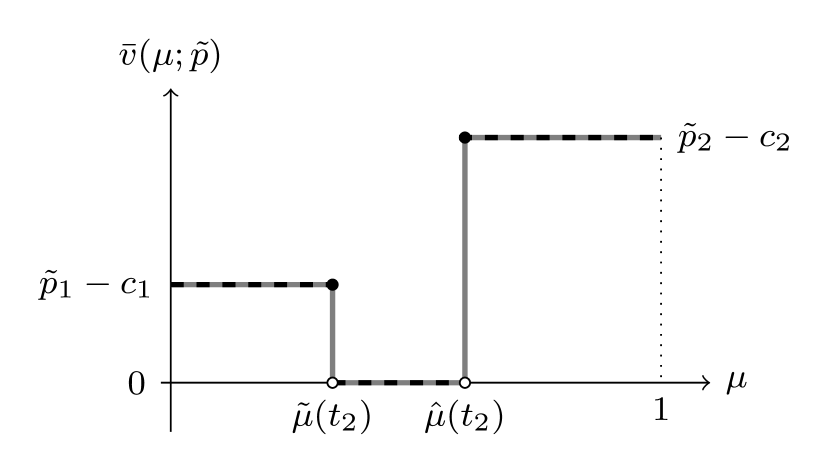
(a) $\bar{v}(\mu;\tilde{p})$

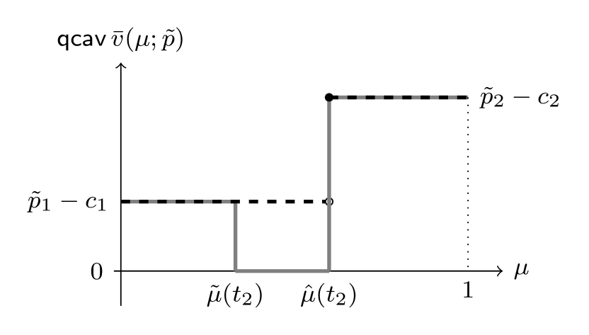
(b) $\operatorname{\mathsf{qcav}}\bar{v}(\mu;\tilde{p})$

Figure 1: The value function $\bar{v}(\cdot,\tilde{p})$ and its quasiconcave envelope $\operatorname{\mathsf{qcav}}\bar{v}(\cdot,\tilde{p})$, as denoted by the dashed lines in Figure 1a and Figure 1b respectively.

2.4 Expert’s equilibrium payoffs

Our solution concept implies that Expert’s equilibrium payoff should be his highest Expert-optimal $p$-equilibrium payoff across all price lists. By 1, Expert’s equilibrium payoff $\operatorname{\mathsf{max}}_{p\in\mathbb{R}^{N}_{+}}U^{E}(p)$ can be written as:

$$\operatorname{\mathsf{max}}_{p\in\mathbb{R}^{N}_{+}}\operatorname{\mathsf{qcav}}\bar{v}(\mu^{0};p).$$ (4)

However, using (4) to calculate Expert’s equilibrium payoffs seems intractable as it requires calculating the quasiconcave envelopes for all $p$. One of our main results is that one can switch the order of the two operators, $\operatorname{\mathsf{max}}_{p}$ and $\operatorname{\mathsf{qcav}}$, in (4) to compute Expert’s equilibrium payoffs. By doing this, the computation of the quasiconcave envelope only needs to be performed once, thus greatly reducing the computational cost. We formally state this result in 1. To introduce some notations, let $\bar{p}_{i}(\mu)\equiv\sum_{k=1}^{i}\mu(t_{k})l_{k}$ be the belief-based monopoly price for treatment $a_{i}$ and let $\pi_{i}(\mu)\equiv\bar{p}_{i}(\mu)-c_{i}$. Given $\bar{p}_{i}(\mu)$, Client is indifferent between $a_{0}$ and $a_{i}$ under belief $\mu$. Furthermore, let ${\bar{\pi}}(\mu)\equiv\operatorname{\mathsf{max}}_{p\in\mathbb{R}_{+}^{N}}\bar{v}(\mu;p)$ be the belief-based profits for Expert under discriminatory pricing. Since Client has unit demand, profits $\bar{\pi}(\mu)$ can be achieved when Expert sets the (belief-based) price list $(\bar{p}_{1}(\mu),\dots,\bar{p}_{N}(\mu))$ and Client chooses some Expert-preferred option:

$$\bar{\pi}(\mu)=\operatorname{\mathsf{max}}\{0,\pi_{1}(\mu),\dots,\pi_{N}(\mu)\}.$$ (5)

Theorem 1.

Expert’s equilibrium payoff is $\operatorname{\mathsf{qcav}}{\bar{\pi}}(\mu^{0})$.

Proof of 1.

See Section A1. ∎

1 can be stated equivalently as

$$\operatorname{\mathsf{max}}_{p\in\mathbb{R}^{N}_{+}}\operatorname{\mathsf{qcav}}\bar{v}(\mu;p)=\operatorname{\mathsf{qcav}}\operatorname{\mathsf{max}}_{p\in\mathbb{R}^{N}_{+}}\bar{v}(\mu;p)\text{ for all $\mu\in\Delta(T)$.}$$ (6)

Equation (6) is nontrivial. As Expert posts the price list before observing the problem type, the price list cannot be contingent on the sent message or Client’s posterior belief. However, the right-hand side of Equation (6), $\operatorname{\mathsf{qcav}}\operatorname{\mathsf{max}}_{p\in\mathbb{R}^{N}_{+}}\bar{v}(\mu;p)$, allows the price list to be contingent on Client’s posterior belief, resulting in weakly higher expected profits for Expert. It follows from some straightforward algebra that $\operatorname{\mathsf{max}}_{p\in\mathbb{R}^{N}_{+}}\operatorname{\mathsf{qcav}}\bar{v}(\mu;p)\leq\operatorname{\mathsf{qcav}}\operatorname{\mathsf{max}}_{p\in\mathbb{R}^{N}_{+}}\bar{v}(\mu;p)$ for all $\mu$.

To prove the other direction, it suffices to find a special price list $p^{\prime}$ such that $\operatorname{\mathsf{qcav}}\bar{v}(\mu;p^{\prime})\geq\operatorname{\mathsf{qcav}}\operatorname{\mathsf{max}}_{p\in\mathbb{R}_{+}^{N}}\bar{v}(\mu;p)$. The key ingredient of our proof is the construction of the desired price list $p^{\prime}$, which essentially consists of monopoly prices targeted at Client’s possible posteriors. Specifically, fix any $\mu^{\prime}\in\Delta(T)$ and let $v^{\prime}\equiv\operatorname{\mathsf{qcav}}\bar{\pi}(\mu^{\prime})$. The quasiconcavification implies that $v^{\prime}$ can be attained by some splitting of $\mu^{\prime}$, say $\set{\mu^{1},\dots,\mu^{K}}$, such that $v^{\prime}=\bar{\pi}(\mu^{k})$ for $k\in\{\,{1},\dots,{K}\,\}$. Moreover, Client adopts a pure strategy of purchasing some treatment under each posterior. 2 formally states this result.

Lemma 2.

For all $\mu\in\Delta(T)$, there exists a splitting of $\mu$, $\{\,{\mu^{1}},\dots,{\mu^{K}}\,\}$ with $K\leq N$, and $K$ different indices $\{i_{1},i_{2},\dots,i_{K}\}$ such that

$$\operatorname{\mathsf{qcav}}\bar{\pi}(\mu)=\bar{\pi}(\mu^{k})=\bar{p}_{i_{k}}(\mu^{k})-c_{i_{k}}\text{ for }k\in\{\,{1},\dots,{K}\,\}.$$ (7)

Proof of 2.

See the proofs for Claims 1 and 2 in Section A1. ∎

Given some splitting $\{\,{\mu^{1}},\dots,{\mu^{K}}\,\}$ satisfying Equation 7, consider the price list $p^{\prime}=(p^{\prime}_{1},\dots,p^{\prime}_{N})$ with $p_{i}^{\prime}=\bar{p}_{i_{k}}(\mu^{{k}})$ if $i\in\set{i_{1},i_{2},\dots,i_{K}}$ and otherwise $p_{i}^{\prime}>l_{N}$. Given the constructed price list $p^{\prime}$, it can be verified that choosing the treatment $a_{i_{k}}$ is optimal for Client under belief $\mu^{k}$, and $u^{E}(a_{i_{k}},p^{\prime})=\bar{\pi}(\mu^{k})=\operatorname{\mathsf{qcav}}\bar{\pi}(\mu^{\prime})$ for all $k\in\{\,{1},\dots,{K}\,\}$. Therefore, the splitting $\{\,{\mu^{1}},\dots,{\mu^{K}}\,\}$ and the payoff $\operatorname{\mathsf{qcav}}\bar{\pi}(\mu^{\prime})$ constitute a $p^{\prime}$-equilibrium outcome when $\mu^{0}=\mu^{\prime}$. The proof sketch concludes.

Indeed, the constructed price list $p^{\prime}$ and $\left(\{\,{\mu^{1}},\dots,{\mu^{K}}\,\},\operatorname{\mathsf{qcav}}\bar{\pi}(\mu^{\prime})\right)$ constitute an equilibrium outcome at prior $\mu^{\prime}$. Our proof implies the existence of some specific kind of equilibria for any prior. An equilibrium is called a Client-worst equilibrium if Client does not benefit from Expert’s services in that equilibrium. When $\operatorname{\mathsf{qcav}}\bar{\pi}(\mu^{0})=\bar{\pi}(\mu^{0})$, there exists a silent Client-worst equilibrium in which Expert sets the monopoly-price list $(\bar{p}_{1}(\mu^{0}),\dots,\bar{p}_{N}(\mu^{0}))$ and reveals no information to Client. When $\operatorname{\mathsf{qcav}}\bar{\pi}(\mu^{0})>\bar{\pi}(\mu^{0})$, the splitting $\{\,{\mu^{1}},\dots,{\mu^{K}}\,\}$ and the constructed $p^{\prime}$ in the proof sketch lead to a non-silent Client-worst equilibrium as stated in Corollary 1.

Corollary 1.

Suppose $\operatorname{\mathsf{qcav}}\bar{\pi}(\mu^{0})>\bar{\pi}(\mu^{0})$. Then there exists a splitting $\{\,{\mu^{1}},\dots,{\mu^{K}}\,\}$ of $\mu^{0}$ for some $K\in[2,N]$, an into function $\varphi:\{1,\dots,K\}\to\{1,\dots,N\}$ and a Client-worst equilibrium in which:

1. The splitting is $\{\,{\mu^{1}},\dots,{\mu^{K}}\,\}$ and $\operatorname{\mathsf{qcav}}\bar{\pi}(\mu^{0})=\bar{\pi}(\mu^{k})$ for each $k\in\{\,{1},\dots,{K}\,\}$;

2. Expert posts the price list $p^{\prime}=(p^{\prime}_{1},\dots,p^{\prime}_{N})$ with $p_{i}^{\prime}=\bar{p}_{\varphi(k)}(\mu^{k})$ if $i\in\{\,{\varphi(1)},\dots,{\varphi(K)}\,\}$ and otherwise $p_{i}^{\prime}>l_{N}$;

3. At each posterior $\mu^{k}$, Client adopts the pure strategy of choosing treatment $a_{\varphi(k)}$.

The geometric characterization presented in 1 suggests that we can calculate Expert’s equilibrium payoffs as if he can set discriminatory prices targeted at Clients with different posteriors. In Section 3, we formalize this intuition by proposing an alternative game in which discriminatory pricing is allowed. Specifically, we show that Expert’s (maximal) equilibrium value remains the same in the alternative game, the proof of which relies heavily on the Client-worst equilibria described in Corollary 1. Additionally, there generally exist many other equilibria besides the Client-worst equilibria described in Corollary 1, including both non-Client-worst equilibria in which Client benefits from Expert’s services and other Client-worst equilibria. In Section 4, we explicitly solve for all equilibria and characterize Client’s possible welfare when $N=2$.

3 Application to previous research

Our characterization of Expert’s equilibrium payoffs $\operatorname{\mathsf{qcav}}\bar{\pi}(\mu^{0})$ can be viewed as Expert’s equilibrium payoffs in an alternative game $\mathcal{G}^{\text{A}}$, where Expert is allowed to use discriminatory pricing instead of posting a uniform price list. This interpretation enables us to apply the geometric characterization to previous works in which Client does not have the full choice right, thereby strengthening the connection between our paper and the literature on credence goods. From a methodological perspective, this application also demonstrates that the existing methods and insights in cheap talk and information design can be leveraged to understand and solve the problems associated with credence goods.

3.1 Alternative game $\mathcal{G}^{\text{A}}$

The alternative game $\mathcal{G}^{\text{A}}$ shares the same $N$-by-$N$ credence goods environment as that of our model, so we do not repeat its description here. Timing of $\mathcal{G}^{\text{A}}$ is as follows: (1) Expert privately observes the problem type $t\in T$; (2) Expert sends a cheap-talk message $m\in M$ to Client; (3) Expert proposes a price list $p\in\mathbb{R}_{+}^{N}$; (4) Client chooses $a\in A$; (5) Players’ payoffs are realized. A perfect bayesian equilibrium (and henceforth equilibrium) of $\mathcal{G}^{\text{A}}$ consists four maps: (i) Expert’s signalling strategy $\sigma^{A}:T\to\Delta(M)$, (ii) Expert’s pricing strategy $p^{A}:T\times M\to\mathbb{R}_{+}^{N}$, (iii) Client’s choice strategy $\rho^{A}:M\times\mathbb{R}_{+}^{N}\to\Delta(A)$, and (iv) Client’s belief updating $\beta^{A}:M\times\mathbb{R}_{+}^{N}\to\Delta(T)$; such that

1. Given $\sigma^{A}$ and $p^{A}$, Client’s posterior belief after observing $m$ and $p$ is obtained from the prior $\mu^{0}$ using Bayes’s rule whenever possible:

   $$\beta^{A}(t_{i}\mid m,p)=\frac{\mu^{0}(t_{i})\sigma^{A}(m\mid t_{i})\Pr(p\mid m,t_{i})}{\sum_{k=1}^{N}\mu^{0}(t_{k})\sigma^{A}(m\mid t_{k})\Pr(p\mid m,t_{k})}$$

   for $t_{i}\in T$, where $\Pr(p\mid m,t_{i})$ takes the value of $1$ if $p^{A}(t_{i},m)=p$ or otherwise $0$. If $\sigma(m|t_{i})=0$ for all $t_{i}\in T$, then Client puts probability one on some problem type of index $i\in\operatorname{\mathsf{arg}}\min_{i}l_{i}-c_{i}$.

2. Given the belief updating $\beta^{A}$, Client’s strategy $\rho^{A}(\cdot\mid m,p)$ after observing $m$ and $p$ is supported on

   $$\operatorname{\mathsf{arg}}\operatorname{\mathsf{max}}_{a\in A}\sum_{t\in T}u^{C}(a,t,p)\beta^{A}(t\mid m,p)$$

   for $m\in M$ and $p\in\mathbb{R}_{+}^{N}$.

3. Given Client’s $\rho^{A}$ and Expert’s $p^{A}$, Expert’s signalling strategy $\sigma^{A}(\cdot\mid t)$ is supported on

   $$\operatorname{\mathsf{arg}}\operatorname{\mathsf{max}}_{m\in M}\sum_{a\in A}\rho^{A}\left(a\mid m,p^{A}(t,m)\right)u^{E}\left(a,p^{A}(t,m)\right)$$

   for $t\in T$;

4. Given Client’s $\rho^{A}$ and sent message $m$, Expert’s pricing strategy satisfies:

   $$p^{A}(t,m)\in\operatorname{\mathsf{arg}}\operatorname{\mathsf{max}}_{p}\sum_{a\in A}\rho^{A}(a\mid m,p)u^{E}(a,p).$$

Say that Expert’s pricing strategy does not signal the problem type if $p^{A}(t,m)=p^{A}(t^{\prime},m)$ for all $m\in M$ and all $t,t^{\prime}\in T$. We argue that as long as the message space is sufficiently rich, it is without loss of generality to focus on equilibria in which Expert’s pricing strategy does not signal the problem type. The reason is that any equilibrium $(\sigma^{A},p^{A},\beta^{A},\rho^{A})$ can be transformed into another equilibrium $(\tilde{\sigma}^{A},\tilde{p}^{A},\tilde{\beta}^{A},\tilde{\rho}^{A})$ that leads to the same outcome, but with a pricing strategy not signalling the problem type. The trick for the transformation is that for any pair $(\sigma^{A},p^{A})$, we can find a more Blackwell-informative signalling strategy $\tilde{\sigma}^{A}$ such that observing both the posted price list and sent message under $({\sigma}^{A},{p}^{A})$ is informationally equivalent for Client to observing the message alone under $\tilde{\sigma}^{A}$. Figure 2 illustrates the transformation process. Figure 2(a) represents the original strategy pair $(\sigma^{A},p^{A})$, and Figure 2(b) represents the transformed strategy pair $(\tilde{\sigma}^{A},\tilde{p}^{A})$. Each node represents a problem type, a sent message or a proposed price list, and the numbers on the paths indicate the transition probabilities. In Figure 2(a), the pricing strategy signals the type information in that $p^{A}(t_{1},m_{1})\neq p^{A}(t_{2},m_{1})$, and Client’s belief will be dependent on the proposed price list after Client observes $m_{1}$. In Figure 2(b), the final nodes and transition probabilities remain unchanged; however, under $\tilde{\sigma}^{A}$ Expert sends four distinct messages indexed by $\zeta(1,1)$, $\zeta(2,3)$, $\zeta(1,2)$ and $\zeta(3,3)$. When observing the message indexed by $\zeta(i,j)$, Client updates her belief as if she observed $m_{i}$ and $p^{j}$ in the situation described by Figure 2(a). Therefore, in the situation described by Figure 2(b), Client’s posterior is independent of the proposed price list, and her posterior and the price list at each final node are the same as in the situation described by Figure 2(a).

Formally, for any equilibrium $(\sigma^{A},p^{A},\beta^{A},\rho^{A})$, let $M^{\prime}\equiv\bigcup_{t\in T}\operatorname{\mathsf{supp}}\sigma^{A}(\cdot\mid t)$ be the set of messages that may be sent under $\sigma^{A}$, and let $P^{\prime}\equiv\set{p^{A}(t,m):t\in T,m\in M^{\prime}}$ be the set of price lists that may be proposed under $(\sigma^{A},p^{A})$. We index the set $P^{\prime}$ by $\{\,{p^{1}},\dots,{p^{K}}\,\}$ and let $p^{k(i,j)}\equiv p^{A}(t_{i},m_{j})$ be the proposed price list under $p^{A}$ given $t_{i}$ and $m_{j}$ where $k(i,j)$ is the index of the price list. Consider an into function $\zeta:M^{\prime}\times P^{\prime}\to M\setminus M^{\prime}$ and a new strategy profile $(\tilde{\sigma}^{A},\tilde{p}^{A},\tilde{\beta}^{A},\tilde{\rho}^{A})$ with

$$\begin{split}\tilde{\sigma}^{A}(m_{\zeta(j,k(i,j))}\mid t_{i})=\sigma^{A}(m_{j}\mid t_{i}),\quad\tilde{p}^{A}(t_{i},m_{\zeta(j,k(i,j))})=p^{k(i,j)}=p^{A}(t_{i},m_{j}),\\ \tilde{\beta}^{A}(m_{\zeta(j,k(i,j))},p^{k(i,j)})=\beta^{A}(m_{j},p^{k(i,j)}),\quad\rho^{A}(a\mid t_{i},m_{\zeta(j,k(i,j))})=\tilde{\rho}^{A}(a\mid t_{i},m_{j}),\end{split}$$

for all $t_{i}\in T$ and all $m_{j}\in M^{\prime}$. Since observing both $m_{j}$ and $p^{k(i,j)}$ under $({\sigma}^{A},{p}^{A})$ is informationally equivalent for Client to observing $m_{\zeta(j,k(i,j))}$ under $(\tilde{\sigma}^{A},\tilde{p}^{A})$, the profile $(\tilde{\sigma}^{A},\tilde{p}^{A},\tilde{\beta}^{A},\tilde{\rho}^{A})$ is an equilibrium in which the pricing strategy does not signal the problem type.

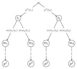
(a) Expert’s strategy pair $({\sigma}^{A},{p}^{A})$

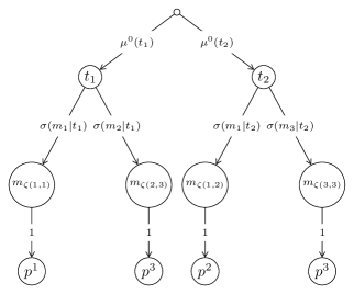
(b) Expert’s strategy pair $(\tilde{\sigma}^{A},\tilde{p}^{A})$

Figure 2: Transforming $(\sigma^{A},p^{A})$ into $(\tilde{\sigma}^{A},\tilde{p}^{A})$ so that the pricing strategy does not signal the problem type

When Expert’s pricing strategy has no signalling effect, Expert’s possible payoffs given Customer’s posterior $\mu$ constitute the interval $[0,\bar{\pi}(\mu)]$ and his value function is exactly $\bar{\pi}(\mu)$. Therefore, Expert’s maximal equilibrium payoffs in $\mathcal{G}^{\text{A}}$ are $\operatorname{\mathsf{qcav}}\bar{\pi}(\mu^{0})$. Moreover, the Client-worst equilibrium described in Corollary 1 can be reinterpreted as an equilibrium of game $\mathcal{G}^{\text{A}}$. We summarize these results in 1.

Proposition 1.

1. Expert’s maximal equilibrium payoffs of $\mathcal{G}^{\text{A}}$ are $\operatorname{\mathsf{qcav}}\bar{\pi}(\mu^{0})$.

2. Suppose $\operatorname{\mathsf{qcav}}\bar{\pi}(\mu^{0})>\bar{\pi}(\mu^{0})$. Then there exists an into function $\varphi:\{1,\dots,K\}\to\{1,...,N\}$ for some integer $K\in[2,N]$ and an equilibrium of $\mathcal{G}^{\text{A}}$ in which

   1. the belief splitting is $\{\,{\mu^{1}},\dots,{\mu^{K}}\,\}$ satisfying $\operatorname{\mathsf{qcav}}\bar{\pi}(\mu^{0})=\bar{\pi}(\mu^{1})=\dots=\bar{\pi}(\mu^{K})$;

   2. at posterior $\mu^{k}\in\{\,{\mu^{1}},\dots,{\mu^{K}}\,\}$, Expert proposes the price list $p^{*}$ with $p^{*}_{i}=\bar{p}_{\varphi(k)}(\mu^{k})$ if $i=\varphi(k)$ and otherwise $p_{i}^{*}>l_{N}$;

   3. Client adopts the pure strategy of purchasing treatment $a_{\varphi(k)}$ at posterior $\mu^{k}$ for $\mu^{k}\in\{\,{\mu^{1}},\dots,{\mu^{K}}\,\}$.

Note that in an equilibrium described in 1(b), Expert essentially restricts Client’s choice set at posterior $\mu^{k}$ by setting prohibitively high prices for all treatments except $a_{\varphi(k)}$. This is analogous to the non-full-choice-right feature in previous credence goods research, in which Client either accepts or rejects Expert’s recommended treatment. Based on this observation, we proceed to show that our geometric characterization can be applied to previous works.

3.2 Fong, Liu, and Wright (2014)

Consider a generalized game of Fong, Liu, and Wright (2014) with $N$ types and $N$ available treatments, which is referred to as $\mathcal{G}^{\text{FLW}}$ from now on. Games $\mathcal{G}^{\text{A}}$ and $\mathcal{G}^{\text{FLW}}$ differ in (i) whether Expert can charge discriminatory prices or not and (ii) whether Expert sends a cheap talk message or makes a treatment recommendation.

Timing of $\mathcal{G}^{\text{FLW}}$ is as follows: (1) Expert posts a price list $p$; (2) Expert privately observes the problem type $t\in T$; (3) Expert recommends some treatment $a_{i}\in A$, where Expert refuses to offer a treatment for Client by recommending $a_{i}=a_{0}$; (4) Client chooses between the recommended treatment $a_{i}$ and $a_{0}$. (5) Players’ payoffs are realized. Following Expert posting some price list $p\in\mathbb{R}^{N}_{+}$, a $p$-equilibrium of $\mathcal{G}^{\text{FLW}}$ consists of: (i) Expert’s recommendation strategy $\gamma^{\text{FLW}}:T\to\Delta(A)$; (ii) Client’s belief updating $\beta^{\text{FLW}}:A\to\Delta(T)$; (iii) Client’s choice strategy $\rho^{\text{FLW}}:A\to\Delta(A)$; such that

1. Given Expert’s recommendation strategy $\gamma^{\text{FLW}}$, Client’s posterior belief after receiving recommendation $a\in A$ is obtained from the prior $\mu^{0}$ using Bayes’s rule:

   $$\beta^{\text{FLW}}(t_{i}\mid a)=\frac{\mu^{0}(t_{i})\gamma^{\text{FLW}}(a\mid t_{i})}{\sum_{k=1}^{N}\mu^{0}(t_{k})\gamma^{\text{FLW}}(a\mid t_{k})}$$

   for $t_{i}\in T$. If $\gamma^{\text{FLW}}(a\mid t_{i})=0$ for all $t_{i}\in T$, then Client puts probability one on some problem type of index $i\in\operatorname{\mathsf{arg}}\min_{i}l_{i}-c_{i}$.

2. Given the belief updating $\beta^{\text{FLW}}$, Client’s strategy $\rho^{\text{FLW}}(\cdot\mid a_{i})$ after receiving recommendation $a_{i}$ is supported on

   $$\operatorname{\mathsf{arg}}\operatorname{\mathsf{max}}_{a\in\set{a_{i},a_{0}}}\sum_{t\in T}u^{C}(a,t,p)\beta^{\text{FLW}}(t\mid a_{i})$$

   for $a_{i}\in A$.

3. Given Client’s strategy $\rho^{\text{FLW}}$, Expert’s recommendation strategy $\gamma^{\text{FLW}}(\cdot\mid t)$ is supported on

   $$\operatorname{\mathsf{arg}}\operatorname{\mathsf{max}}_{a_{i}\in A}\sum_{a\in\set{a_{0},a_{i}}}\rho^{\text{FLW}}(a\mid a_{i})u^{E}(a,p)$$

   for $t\in T$.

The solution concept of $\mathcal{G}^{\text{FLW}}$ is the Expert-optimal perfect bayesian equilibrium, referred as an equilibrium of $\mathcal{G}^{\text{FLW}}$. It follows that Expert’s equilibrium payoffs in $\mathcal{G}^{\text{FLW}}$ are his highest $p$-equilibrium payoffs among all $p\in\mathbb{R}^{N}_{+}$. We argue that Expert’s equilibrium payoffs in $\mathcal{G}^{\text{FLW}}$ are also $\operatorname{\mathsf{qcav}}\bar{\pi}(\mu^{0})$. On the one hand, any $p$-equilibrium of $\mathcal{G}^{\text{FLW}}$ corresponds to an equilibrium of $\mathcal{G}^{\text{A}}$ in which Expert’s ex ante payoffs are unchanged. Specifically, whenever Expert sets $p^{\prime}$ and recommends $a_{i}$ in $\mathcal{G}^{\text{FLW}}$, we can replace it with Expert sending message $m_{i}$ and proposing $\tilde{p}^{\prime}$ in $\mathcal{G}^{\text{A}}$, with $\tilde{p}^{\prime}_{i}=p^{\prime}_{i}$ and $\tilde{p}^{\prime}_{j}>l_{N}+1$ for all $j\neq i$. This implies that Expert’s equilibrium payoffs in $\mathcal{G}^{\text{FLW}}$ must be weakly lower than Expert’s maximal equilibrium payoffs in $\mathcal{G}^{\text{A}}$. On the other hand, any Client-worst equilibrium of $\mathcal{G}^{\text{A}}$ described in 1(b) also corresponds to some $\tilde{p}^{*}$-equilibrium of $\mathcal{G}^{\text{FLW}}$ in which Expert’s ex ante payoffs remain unchanged. Specifically, whenever Expert sends message $m_{\varphi(k)}$ and proposes $p^{*}$ with $p^{*}_{\varphi(k)}=\bar{p}_{\varphi(k)}(\mu^{k})$ in some Client-worst equilibrium of $\mathcal{G}^{\text{A}}$, we can replace it with Expert recommending treatment $a_{\varphi(k)}$ in $\mathcal{G}^{\text{A}}$, after posting the uniform price list $\tilde{p}^{*}$ with $\tilde{p}^{*}_{i}=\bar{p}_{\varphi(k)}(\mu^{k})$ if $i=\varphi(k)$ for some $k\in\{\,{1},\dots,{K}\,\}$ or otherwise $\tilde{p}^{*}_{i}>l_{N}$.

Proposition 2.

Expert’s equilibrium payoffs of $\mathcal{G}^{\text{FLW}}$ are $\operatorname{\mathsf{qcav}}\bar{\pi}(\mu^{0})$.

It is worth noting that 2 cannot be derived directly from a comparison between $\mathcal{G}^{\text{FLW}}$ and our main model in Section 2. While an equilibrium of our main model described in Corollary 1 can also be reinterpreted as some $p$-equilibrium of $\mathcal{G}^{\text{FLW}}$, we can only conclude that Expert’s equilibrium payoffs in $\mathcal{G}^{\text{FLW}}$ are weakly higher than $\operatorname{\mathsf{qcav}}\bar{\pi}(\mu^{0})$. Furthermore, in contrast to our main model, Expert in $\mathcal{G}^{\text{FLW}}$ has the advantage of restricting Client’s choice set by making a treatment recommendation. Therefore, it remains uncertain whether Expert’s equilibrium payoffs in $\mathcal{G}^{\text{FLW}}$ are strictly higher than $\operatorname{\mathsf{qcav}}\bar{\pi}(\mu^{0})$.

4 Binary case

In this section, we focus on the binary case when $N=2$ and explicitly solve for all equilibria. We assume that problems of type $t_{2}$ are more cost-effective to resolve (i.e., $l_{2}-c_{2}>l_{1}-c_{1}$). The equilibria for the opposite scenario, where resolving problems of type $t_{1}$ is more cost-effective, can be derived in a similar manner.

To begin, we calculate Expert’s equilibrium payoffs in the binary case. Let $\mu^{0}=(1-q,q)$, where $q\equiv\mu^{0}(t_{2})$ is the probability weight put on $t_{2}$ under the prior belief. In Figure 3, we plot the belief-based profits function $\bar{\pi}(\mu^{0})$, represented by the dashed lines, and its quasiconcave envelope $\operatorname{\mathsf{qcav}}\bar{\pi}(\mu^{0})$, represented by the solid lines. Specifically, there are two possible cases of $\bar{\pi}(\mu^{0})$. If $l_{2}\geq\frac{c_{2}-c_{1}}{l_{1}-c_{1}}l_{1}$, Client will always purchase one of the two treatments and $\bar{\pi}(\mu^{0})>0$ for all $\mu^{0}$ (Figure 3a). Otherwise, Client will not purchase either treatment and $\bar{\pi}(\mu^{0})=0$ given that $q$ is intermediate (Figure 3b). Both cases lead to the same quasiconcave envelope: $\operatorname{\mathsf{qcav}}\bar{\pi}(\mu^{0})$ is flat for $0<q<\hat{q}\equiv\frac{c_{2}-c_{1}}{l_{2}-l_{1}}$ and then increases linearly to $l_{2}-c_{2}$ as $q$ approaches $1$.

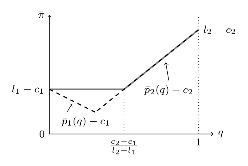
(a) Case I: $l_{2}\geq\frac{c_{2}-c_{1}}{l_{1}-c_{1}}l_{1}$

(b) Case II: $l_{2}<\frac{c_{2}-c_{1}}{l_{1}-c_{1}}l_{1}$

Figure 3: Possible cases of $\bar{\pi}(q)$ and $\operatorname{\mathsf{qcav}}\bar{\pi}(q)$, represented by the dashed lines and the solid lines respectively.

We say communication benefits Expert if $\operatorname{\mathsf{qcav}}\bar{\pi}(\mu^{0})>\bar{\pi}(\mu^{0})$. Figure 3 implies that in the binary case, communication benefits Expert if and only if $q\in(0,\hat{q})$. It follows that when $\mu^{0}(t_{2})\geq\hat{q}$, there exists a silent Client-worst equilibrium in which Expert charges the monopoly price for treatment $a_{2}$ and reveals no information to Client. Indeed, this silent equilibrium is unique when $q>\hat{q}$.

Proposition 3.

When $q\in(\hat{q},1]$, there exists a unique equilibrium. In that equilibrium, Expert sets $p_{2}^{*}=ql_{2}+(1-q)l_{1}$ and $p_{1}^{*}>l_{1}$ and does not reveal any information, and Client chooses $a_{2}$.

Proof.

Assume by contradiction that there exists an equilibrium outcome $(\{\mu^{1},...,\mu^{K}\},\bar{\pi}(\mu^{0}),p^{*})$ with $K^{*}\geq 2$ and $\bar{\pi}(\mu^{0})=q(l_{2}-l_{1})+(l_{1}-c_{2})$. Then there exists some posterior $\mu^{k}\in\{\mu^{1},...,\mu^{K}\}$ such that $\mu^{k}(t_{2})<q$, and thus $\bar{\pi}(\mu^{k})<\bar{\pi}(\mu^{0})$. Contradiction. ∎

Now we solve for the equilibria when $q\in(0,\hat{q})$. As shown in Figure 3, Expert’s equilibrium payoffs will be $l_{1}-c_{1}$ for any $q\in(0,\hat{q})$. Let $\set{\mu^{1},\dots,\mu^{K^{*}}}$ be the splitting of $\mu^{0}$ in some equilibrium outcome with $\mu^{1}(t_{2})<\dots<\mu^{K^{*}}(t_{2})$. Since $\operatorname{\mathsf{qcav}}\bar{\pi}(\mu^{0})>\bar{\pi}(\mu^{0})$, all equilibria must be non-silent and $K^{*}\geq 2$. Since $\mu^{1}(t_{2})<\hat{q}$, Expert must set $\mu^{1}(t_{2})=0$ and $p_{1}=l_{1}$ to obtain the payoff of $l_{1}-c_{1}$ at posterior $\mu^{1}$. Additionally, there does not exist any other posterior whose probability weight on $t_{2}$ is strictly fewer than $\hat{q}$: $\mu^{k}(t_{2})\geq\hat{q}$ for all $k\geq 2$. Otherwise, if there exists some $k$ such that $\mu^{k}(t_{2})\in(0,\hat{q})$, then Expert’s payoffs at posterior $\mu^{k}$ must be strictly less than $l_{1}-c_{1}$.

Lemma 3.

Suppose $q\in(0,\hat{q})$ and let $\set{\mu^{1},\dots,\mu^{K^{*}}}$ be the belief splitting in some equilibrium outcome with $\mu^{1}(t_{2})<\dots<\mu^{K^{*}}(t_{2})$. Then $K^{*}\geq 2$ and in all equilibria, Expert sets $p_{1}^{*}=l_{1}$, $\mu^{1}(t_{2})=0$, and $\mu^{k}(t_{2})\geq\hat{q}$ for all $k\in\{\,{2},\dots,{K^{*}}\,\}$.

We characterize all equilibria based on 3. In contrast to the case when $q>\hat{q}$, multiple equilibria exist when $q\in(0,\hat{q})$. Furthermore, a belief splitting of $\mu^{0}$, $\{\,{\mu^{1}},\dots,{\mu^{K^{*}}}\,\}$, can appear in some equilibrium outcome as long as $\mu^{1}(t_{2})=0$ and $\mu^{k}(t_{2})\geq\hat{q}$ for all $k\in\{\,{2},\dots,{K^{*}}\,\}$.

Proposition 4.

Suppose $q\in(0,\hat{q})$. Fix a splitting of $\mu^{0}$, $\{\,{\mu^{1}},\dots,{\mu^{K^{*}}}\,\}$, that satisfies $K^{*}\geq 2$, $\mu^{1}(t_{2})=0$ and $\mu^{k}(t_{2})\geq\hat{q}$ for $k\in\{\,{2},\dots,{K^{*}}\,\}$. Then $\{\,{\mu^{1}},\dots,{\mu^{K^{*}}}\,\}$ appears in some equilibrium outcome. Specifically,

1. When ${K^{*}}>2$, there exists a unique equilibrium with the splitting being $\{\,{\mu^{1}},\dots,{\mu^{K^{*}}}\,\}$. In that equilibrium, Expert sets $p_{1}^{*}=l_{1}$ and $p_{2}^{*}=c_{2}+l_{1}-c_{1}$, and Client chooses $a_{1}$ at posterior $\mu^{1}$ and chooses $a_{2}$ at posterior $\mu^{k}$ for $k\in\{\,{2},\dots,{K^{*}}\,\}$.

2. When $K^{*}=2$ and $\mu^{2}(t_{2})>\hat{q}$, there exist two equilibria with the splitting being $\set{\mu^{1},\mu^{2}}$. One is a Client-worst equilibrium, in which Expert sets $p_{1}^{*}=l_{1}$ and $p_{2}^{*}=l_{1}+\mu^{2}(t_{2})(l_{2}-l_{1})$, and Client chooses $a_{1}$ at posterior $\mu^{1}$ and, at posterior $\mu^{2}$, Client chooses $a_{2}$ with probability $\frac{l_{1}-c_{1}}{l_{1}+\mu^{2}(t_{2})(l_{2}-l_{1})-c_{2}}$ and chooses $a_{0}$ with the complementary probability. The other is a non-Client-worst equilibrium, in which Expert sets $p^{*}_{1}=l_{1}$ and $p^{*}_{2}=c_{2}+l_{1}-c_{1}$, and Client chooses $a_{1}$ at posterior $\mu^{1}$ and chooses $a_{2}$ at posterior $\mu^{2}$.

3. When $K^{*}=2$ and $\mu^{2}(t_{2})=\hat{q}$, there exists a unique equilibrium with the splitting being $\set{\mu^{1},\mu^{2}}$. In that equilibrium, Expert sets $p_{1}^{*}=l_{1}$ and $p_{2}^{*}=c_{2}+l_{1}-c_{1}$, and Client chooses $a_{1}$ at posterior $\mu^{1}$ and chooses $a_{2}$ at posterior $\mu^{2}$.

Proof.

See Section A2. ∎

When the belief splitting contains more than two posteriors, 4(a) implies that there is a unique corresponding equilibrium. In that equilibrium, Expert charges equal margins for both treatments and Client adopts a pure strategy, choosing $a_{1}$ at posterior $\mu^{1}$ or otherwise choosing $a_{2}$. To demonstrate this, consider Client’s optimal response at posterior $\mu^{k}$ for some $k\in\{\,{2},\dots,{K}\,\}$. First, Client will never choose $a_{1}$ at $\mu^{k}$ since $\mu^{k}(t_{1})l_{1}<l_{1}=p_{1}^{*}$. Client will adopt a pure strategy of choosing $a_{0}$ when $p_{2}>\mu^{k}(t_{1})l_{1}+\mu^{k}(t_{2})l_{2}$ or of choosing $a_{2}$ when $p_{2}<\mu^{k}(t_{1})l_{1}+\mu^{k}(t_{2})l_{2}$. Furthermore, Client may mix between $a_{0}$ and $a_{2}$ when these two options yield the same payoff, $p_{2}=\mu^{k}(t_{1})l_{1}+\mu^{k}(t_{2})l_{2}$. It follows that once Client mixes between $a_{0}$ and $a_{2}$ at $\mu^{k}$, she must adopt a pure strategy of choosing $a_{0}$ or $a_{2}$ at any other posterior $\mu^{k^{\prime}}$ with $k^{\prime}\geq 2$. However, in that case, Expert will not be indifferent between sending message $m_{k}$ and $m_{k^{\prime}}$. Therefore, in any equilibrium Client chooses $a_{2}$ at $\mu^{k}$ for $k\geq 2$, and the equal-margin condition must hold, $p_{2}-c_{2}=l_{1}-c_{1}$.

When the belief splitting contains two posteriors and $\mu^{2}(t_{2})>\hat{q}$, 4(b) implies that there are precisely two corresponding equilibria. One equilibrium requires Client to mix between $a_{0}$ and $a_{2}$ at posterior $\mu^{2}$, while in the other equilibrium Expert set equal margins over both treatments and Client chooses $a_{2}$ at $\mu^{2}$. The analysis mirrors that of the case when $K^{*}>2$, and the existence of the additional equilibrium where Client adopts a mixed strategy arises from the fact that only one posterior exists such that $\mu^{k}(t_{2})\geq\hat{q}$. When $\mu^{2}(t_{2})=\hat{q}$, $\frac{l_{1}-c_{1}}{l_{1}+\mu^{2}(t_{2})(l_{2}-l_{1})-c_{2}}=1$ and the two equilibria coincide as in 4(c).

When discussing equilibria with equal margins, previous works in the credence goods literature mostly focus on the honest equilibria (e.g., Fong, Liu, and Wright, 2014; Dulleck and Kerschbamer, 2006) in which Expert always reveals the true problem type. This corresponds to the equilibrium with $K^{*}=2$ and $\mu^{2}=(0,1)$ of our binary case. However, we also find many other equilibria with equal margins, in which Expert does not always reveal the true problem type. The identified equilibria in 4 with $K^{*}=2$ and $\mu^{2}(t_{2})\in[\hat{q},1]$ can be translated into equilibria of $\mathcal{G}^{\text{FLW}}$ in which Expert adopts a partial–overtreatment strategy. Specifically, Expert always recommends treatment $a_{2}$ when $t=t_{2}$ and mixes between recommending treatment $a_{1}$ and $a_{2}$ when $t=t_{1}$, such that $\mu^{2}(t_{2})\in[\hat{q},1]$; Client’s posterior is $\mu^{1}$ ($\mu^{2}$) given the recommendation $a_{1}$ ($a_{2}$), and always accepts Expert’s recommendation.

4.1 Value of Expert’s services

Under the same prior, all equilibria yield the same payoff for Expert. However, they may have different implications for welfare since Client’s equilibrium payoffs can vary. We use the value of Expert’s services for Client as proxy for Client’s welfare. Since the potential social surplus is $S(\mu^{0})\equiv(1-q)(l_{1}-c_{1})+q(l_{2}-c_{2})$ where $q=\mu^{0}(t_{2})$, the value of Expert’s services cannot exceed $S(\mu^{0})-\operatorname{\mathsf{qcav}}\bar{\pi}(\mu^{0})$. We discuss Client’s possible welfare among all equilibria and demonstrate that the value of Expert’s services for Client can take any value in the interval $\big{[}0,S(\mu^{0})-\operatorname{\mathsf{qcav}}\bar{\pi}(\mu^{0})\big{]}$ when $q\in(0,\hat{q})$. When $q>\hat{q}$, there exists a unique equilibrium (3), in which the value of Expert’s services is zero.

Since a Client-worst equilibrium always exists (Corollary 1), the lower bound for the value of Expert’s services is attainable for any $q\in(0,\hat{q})$. On the other hand, consider the non-Client-worst equilibria when the splitting contains two posteriors, $\set{\mu^{1},\mu^{2}}$, as described in 4(b). Among these equilibria, the value of Expert’s services is given by

$$q(l_{2}-l_{1})-\frac{q}{\mu^{2}(t_{2})}(c_{2}-c_{1}).$$

As $\mu^{2}(t_{2})$ goes from $\hat{q}$ to $1$, the value of Expert’s services changes monotonically from $0$ to $q[(l_{2}-l_{1})-(c_{2}-c_{1})]=S(\mu^{0})-\operatorname{\mathsf{qcav}}\bar{\pi}(\mu^{0})$.

Proposition 5.

For $q\in(0,\hat{q})$, the values of Expert’s services for Client among all equilibria constitute the interval $[0,S(\mu^{0})-\operatorname{\mathsf{qcav}}\bar{\pi}(\mu^{0})]$.

5 When does communication benefit Expert?

Recall that when $N=2$, Expert benefits from communication if and only if $\mu^{0}(t_{2})\in(0,\hat{q})$. In this section, we generalize this observation and provide a necessary and sufficient condition for when communication benefits Expert. Denote by $s_{(k)}$ the $k$-th highest element of the set $\{\,{s_{1}},\dots,{s_{N}}\,\}$, where $s_{i}=l_{i}-c_{i}$ is the social surplus of resolving a problem of type $t_{i}$. As demonstrated in 2, the desired condition concerns the second-highest surplus, $s_{(2)}$.

Theorem 2.

For all $\mu^{0}$ in the interior of $\Delta(T)$, Expert benefits from communication (i.e., $\operatorname{\mathsf{qcav}}\bar{\pi}(\mu^{0})>\bar{\pi}(\mu^{0})$) if and only if

$$\bar{\pi}(\mu^{0})<s_{(2)}.$$ (8)

Proof.

See Section A3. ∎

Note that the prerequisite in 2 of the prior being interior is not a restriction. Whenever $\mu^{0}$ is not in the interior of $\Delta(T)$, the $N$ by $N$ credence goods setup can be reduced to an $N^{\prime}$ by $N^{\prime}$ setup with a smaller type space $T^{\prime}\subset T$, where the prior will be in the interior of $\Delta(T^{\prime})$. We can compute the corresponding second-highest potential surplus in the reduced setup and then apply 2.

We illustrate 2 when $N=3$ and $s_{1}<s_{2}<s_{3}$ in Figure 4, where Figure 4(a) and Figure 4(b) illustrate $\bar{\pi}(\mu)$ and $\operatorname{\mathsf{qcav}}\bar{\pi}(\mu)$ respectively. In Figure 4(b), the area filled with line patterns, together with the bold lines, indicates the intersection of the graphs of $\bar{\pi}(\mu)$ and $\operatorname{\mathsf{qcav}}\bar{\pi}(\mu)$. According to 2, communication does not benefit Expert for those interior priors sufficiently close to the extreme belief $e^{3}$ such that $\bar{\pi}(\mu^{0})\geq s_{2}$. The area with line patterns in Figure 4(b) confirms this prediction.

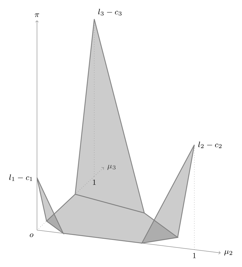
(a) $\bar{\pi}(\mu^{0})$

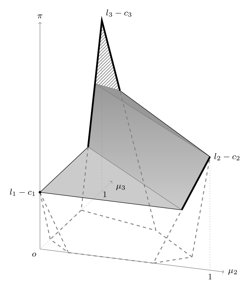
(b) $\operatorname{\mathsf{qcav}}\bar{\pi}(\mu^{0})$

Figure 4: Surfaces of $\bar{\pi}(\mu^{0})$ and $\operatorname{\mathsf{qcav}}\bar{\pi}(\mu^{0})$ when $N=3$ and $s_{2}<s_{3}$.

A direct corollary of 2 is that when $s_{(1)}=s_{(2)}$, Expert benefits from communication for all interior priors. Figure 5 illustrates this situation when $N=3$ and $l_{1}-c_{1}<l_{2}-c_{2}=l_{3}-c_{3}$, where Figure 5(a) and Figure 5(b) illustrate $\bar{\pi}(\mu)$ and $\operatorname{\mathsf{qcav}}\bar{\pi}(\mu)$ respectively. In this case, the equality of $\bar{\pi}(\mu)$ and $\operatorname{\mathsf{qcav}}\bar{\pi}(\mu)$ only occurs at the boundary of $\Delta(T)$, denoted by the bold lines in Figure 5(b).

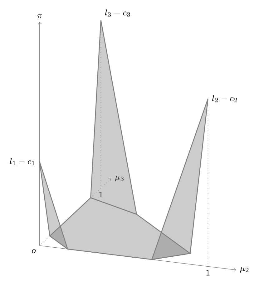
(a) $\bar{\pi}(\mu^{0})$

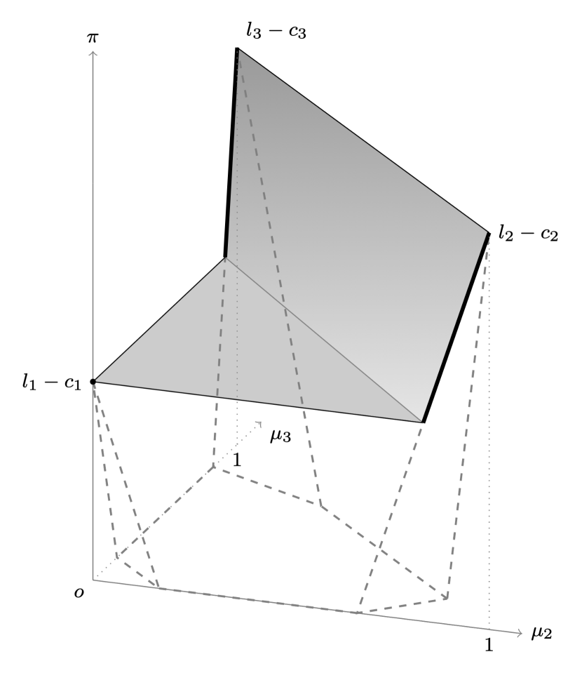
(b) $\operatorname{\mathsf{qcav}}\bar{\pi}(\mu^{0})$

Figure 5: Surfaces of $\bar{\pi}(\mu^{0})$ and $\operatorname{\mathsf{qcav}}\bar{\pi}(\mu^{0})$ when $N=3$ and $s_{2}=s_{3}$.

6 Concluding remarks

This paper is motivated by the observation that in many credence goods markets, the clients possess the full choice right. With this motivation, we study a credence goods model in which the expert sends a cheap-talk message to the client, and then the client self-selects her most desired treatment. We adopt the belief-based approach and provide a geometric characterization of the expert’s equilibrium payoffs. Based on that characterization, we explicitly solve for all the equilibria in the binary case. One implication of our study is that, by considering a general setting, the existing methods and insights in information design and cheap talk can be used to understand and solve the credence goods problems.

As the first paper on credence goods that allows strategic information transmission in the client-expert interaction, this paper has identified a number of areas for future research. For instance, while we have proved the existence of Client-worst equilibrium, we only characterize all the equilibria in the binary case. It would be beneficial for future research to further explore the possible equilibrium outcomes in a different setting. On the other hand, it would also be intriguing to study an alternative communication protocol apart from cheap talk in the credence goods setting. For example, one may consider some communication protocol between cheap talk and bayesian persuasion. Such a framework has the potential to provide insights to many stylized facts in credence-goods markets.

Appendix A Appendix: omitted proofs

A1 Proof of 1

Recall that $\bar{p}_{i}(\mu)\equiv\sum_{k=1}^{i}\mu_{k}l_{k}$ is the monopoly price for treatment $a_{i}$ under belief $\mu$ and ${\bar{\pi}}(\mu)\equiv\operatorname{\mathsf{max}}_{p}\bar{v}(\mu;p)$ denotes Expert’s (belief-based) profits given Client’s belief $\mu$. Since Client has unit demand,

$$\bar{\pi}(\mu)=\operatorname{\mathsf{max}}\{0,\pi_{1}(\mu),\dots,\pi_{N}(\mu)\}\text{ where $\pi_{i}(\mu)=\bar{p}_{i}(\mu)-c_{i}$ for each $i$. }$$ (9)

The belief-based profits function $\bar{\pi}(\mu)$ allows a straightforward geometrical interpretation. A point is a belief plus a value, $(\mu,v)\in\mathbb{R}^{N+1}$. For each $i\in\{\,{1},\dots,{N}\,\}$, the set $\set{(\mu,v):v=\pi_{i}(\mu)}$ is a hyperplane in $\mathbb{R}^{N+1}$, and we use $\pi_{i}(\mu)$ to refer to this hyperplane. Equation 9 implies that $\bar{\pi}(\mu)$ is the upper envelope of the $N+1$ hyperplanes. It can be verified that $\bar{\pi}(\mu)$ is continuous and convex; furthermore, if $\{\,{\mu^{1}},\dots,{\mu^{K}}\,\}$ is a splitting of $\mu$ with $\mu=\sum_{k=1}^{K}\lambda_{k}\mu^{k}$, then

$$\bar{\pi}(\mu)\leq\sum_{k=1}^{K}\lambda_{k}\bar{\pi}(\mu^{k})$$ (10)

and the equality of (10) holds if and only if the $K+1$ points, $(\mu,\bar{\pi}(\mu))$ and $\left(\mu^{k},\bar{\pi}(\mu^{k})\right)$ for $k\in\{\,{1},\dots,{K}\,\}$, are all on the same hyperplane $\pi_{i}(\mu)$ for some $i\in\{\,{1},\dots,{N}\,\}$.

Throughout the proof, we use $\operatorname{\mathsf{max}}_{p}$ as an abbreviation for $\operatorname{\mathsf{max}}_{p\in\mathbb{R}_{+}^{N}}$ and let $\mu_{i}\equiv\mu(t_{i})$ for all $i\in\{\,{1},\dots,{N}\,\}$.

Step 1

$\operatorname{\mathsf{max}}_{p}\operatorname{\mathsf{qcav}}\bar{v}(\mu;p)\leq\operatorname{\mathsf{qcav}}\operatorname{\mathsf{max}}_{p}\bar{v}(\mu;p)$ for all $\mu\in\Delta(T)$.

For all ${p\in\mathbb{R}^{N}_{+}}$ and $\mu\in\Delta(T)$, it follows from $\bar{v}(\mu;p)\leq\operatorname{\mathsf{max}}_{p}\bar{v}(\mu;p)$ that $\operatorname{\mathsf{qcav}}\bar{v}(\mu;p)\leq\operatorname{\mathsf{qcav}}\operatorname{\mathsf{max}}_{p}\bar{v}(\mu;p)$. Therefore, $\operatorname{\mathsf{max}}_{p}\operatorname{\mathsf{qcav}}\pi(\mu;p)\leq\operatorname{\mathsf{qcav}}\operatorname{\mathsf{max}}_{p}\pi(\mu;p)$.

Step 2

$\operatorname{\mathsf{max}}_{p}\operatorname{\mathsf{qcav}}\bar{v}(\mu;p)\geq\operatorname{\mathsf{qcav}}\operatorname{\mathsf{max}}_{p}\bar{v}(\mu;p)$ for all $\mu\in\Delta(T)$.

It suffices to show that for any $\mu^{\prime}\in\Delta(T)$, there exists some price list $p^{\prime}\in\mathbb{R}^{N}_{+}$ such that

$$\operatorname{\mathsf{qcav}}\bar{v}(\mu^{\prime};p^{\prime})\geq\operatorname{\mathsf{qcav}}\bar{\pi}(\mu^{\prime}).$$ (11)

Let $v^{\prime}\equiv\operatorname{\mathsf{qcav}}\bar{\pi}(\mu^{\prime})$. When $\bar{\pi}(\mu^{\prime})=v^{\prime}$, inequality (11) holds by setting $p^{\prime}\in\operatorname{\mathsf{arg}}\operatorname{\mathsf{max}}_{p}\pi(\mu^{\prime},p)$. From now on, we focus on the case when $v^{\prime}>\bar{\pi}(\mu^{\prime})$. By Corollary 1 and Theorem 2 of Lipnowski and Ravid (2020),

$$\begin{split}\operatorname{\mathsf{qcav}}\bar{\pi}(\mu^{\prime})=&\operatorname{\mathsf{max}}_{\{\,{\mu^{1}},\dots,{\mu^{K}}\,\}}\min\{\bar{\pi}(\mu^{1}),\dots\bar{\pi}(\mu^{K})\}\\ \text{subject to }\quad&\text{ $\{\,{\mu^{1}},\dots,{\mu^{K}}\,\}$ is a splitting of $\mu^{\prime}$}.\end{split}$$ (12)

Claim 1.

If $v^{\prime}>\bar{\pi}(\mu^{\prime})$, then there exists a splitting of $\mu^{\prime}$—$\{\,{\mu^{1}},\dots,{\mu^{K}}\,\}$—such that $\bar{\pi}(\mu^{k})=v^{\prime}$ for all $\mu^{k}\in\{\mu^{1},\dots,\mu^{K}\}$.

Proof.

Let $\{\,{\mu^{1}},\dots,{\mu^{K}}\,\}$ be a maximizer to program (12) and then $\bar{\pi}(\mu^{i})\geq v^{\prime}$ for all $i\in\{\,{1},\dots,{K}\,\}$. It suffices to show that whenever $\bar{\pi}(\mu^{k})>v^{\prime}$ for some $k$, then there exists some belief $\tilde{\mu}^{k}$ such that $\bar{\pi}(\tilde{\mu}^{k})=v^{\prime}$ and the set $\set{\mu^{1},\dots,\mu^{k-1},\tilde{\mu}^{k},\mu^{k+1},\dots,\mu^{K}}$ is a splitting of $\mu^{\prime}$. Since $\bar{\pi}(\cdot)$ is continuous and $\bar{\pi}(\mu^{k})>v^{\prime}>\bar{\pi}(\mu^{\prime})$, there exists $\tilde{\mu}^{k}=\lambda\mu^{\prime}+(1-\lambda)\mu^{k}$ for some $\lambda\in(0,1)$ such that $\bar{\pi}(\tilde{\mu}^{k})=v^{\prime}$. Suppose $\sum_{i=1}^{K}\lambda_{i}\mu^{i}=\mu^{\prime}$. Clearly, $\set{\mu^{1},\dots,\mu^{k-1},\tilde{\mu}^{k},\mu^{k+1},\dots,\mu^{K}}$ is a splitting of $\mu^{\prime}$ since $\mu^{\prime}=\sum_{i\neq k}\frac{\lambda_{i}(1-\lambda)}{\lambda\lambda_{k}+1-\lambda}\mu^{i}+\frac{\lambda_{k}}{\lambda\lambda_{k}+1-\lambda}\tilde{\mu}^{k}$. ∎

Based on 1, we further show that there exist a splitting, $\{\,{\mu^{1}},\dots,{\mu^{K}}\,\}$ and $K$ different numbers, $\{\,{i_{1}},\dots,{i_{K}}\,\}$ such that $\bar{\pi}(\mu^{k})=\bar{p}_{i_{k}}(\mu^{k})-c_{i_{k}}=v^{\prime}$ for each $k\in\{\,{1},\dots,{K}\,\}$. We formally state this result below.

Claim 2.

If $v^{\prime}>\bar{\pi}(\mu^{\prime})$, then there exists a splitting of $\mu^{\prime}$, $\{\,{\mu^{1}},\dots,{\mu^{K}}\,\}$ with $K\leq N$, such that $\bar{\pi}(\mu^{k})=\bar{p}_{i_{k}}(\mu^{k})-c_{i_{k}}=v^{\prime}$ for $K$ different $\{i_{1},\dots,i_{K}\}$.

Proof.

By 1, there exists a splitting $\{\mu^{1},\dots,\mu^{L}\}$ with $\sum_{i=1}^{L}\lambda_{i}\mu^{i}=\mu^{\prime}$ satisfying $\bar{\pi}(\mu^{\ell})=v^{\prime}$ for each $\ell\in\{\,{1},\dots,{L}\,\}$. By Equation 9, for each $\ell$ there exists some $i_{\ell}$ such that $\bar{\pi}(\mu^{\ell})=\bar{p}_{i_{\ell}}(\mu^{\ell})-c_{i_{\ell}}$. The mapping

$$\begin{split}\eta:&\{\,{1},\dots,{L}\,\}\to\{\,{1},\dots,{N}\,\}\\ &\ell\mapsto i_{\ell}\end{split}$$

induces a partition of the set $\{\,{1},\dots,{L}\,\}$. Denote by $K(\leq N)$ the number of induced partitions. For the $k$-th partition $\{\,{k_{1}},\dots,{k_{J}}\,\}$, define $\tilde{\mu}^{i_{k}}\equiv\frac{\sum_{j=1}^{J}\lambda_{k_{j}}\mu^{k_{j}}}{\sum_{j=1}^{J}\lambda_{k_{j}}}$. It follows that $\{\tilde{\mu}^{i_{1}},\dots,\tilde{\mu}^{i_{K}}\}$ is also a splitting of $\mu^{\prime}$. Since $\bar{p}_{i_{k}}(\mu)-c_{i_{k}}$ is an affine function of $\mu$, we have $\bar{p}_{i_{k}}(\tilde{\mu}^{i_{k}})-c_{i_{k}}=v^{\prime}$. ∎

By 2, there exist an into function $\varphi:\{\,{1},\dots,{K}\,\}\to\{\,{1},\dots,{N}\,\}$ and a splitting $\{\mu^{1},...,\mu^{K}\}$ of $\mu^{\prime}$ such that

$$\bar{\pi}(\mu^{k})=\bar{p}_{\varphi(k)}(\mu^{k})-c_{\varphi(k)}=v^{\prime},\text{ $\forall k\in\{\,{1},\dots,{K}\,\}$.}$$ (13)

We show that the desired inequality (11) holds by setting $p^{\prime}=(p^{\prime}_{1},\dots,p^{\prime}_{N})$ with

$$p^{\prime}_{i}=\begin{cases}\bar{p}_{\varphi(k)}(\mu^{k}),&\text{if }i\in\{\,{\varphi(1)},\dots,{\varphi(K)}\,\};\\ p_{N}+1,&\text{otherwise}.\end{cases}$$ (14)

Let $U(a;\mu,p)\equiv\mathbb{E}_{\mu}u^{C}(a,t,p)$ be Client’s expected payoff from $a\in A$ given $\mu$ and $p$. It suffices to check that under $\mu^{k}$ and $p^{\prime}$, choosing $a_{{\varphi(k)}}$ is Client’s optimal response for $k\in\{\,{1},\dots,{K}\,\}$. If that were true, $\bar{v}(\mu^{k};p^{\prime})\geq u^{E}(a_{{\varphi(k)}},p^{\prime})=v^{\prime}$ for each $k$ and the LHS of inequality (11) would be weakly greater than $v^{\prime}$. The proof concludes by verifying 3 below. Note that we only need to check that Client prefers $a_{\varphi(k)}$ to $a_{\varphi(\ell)}$ for $\varphi(\ell)\in\{\,{\varphi(1)},\dots,{\varphi(K)}\,\}$. The reason is that $p^{\prime}_{j}$ is prohibitively high for $j\not\in\{\,{\varphi(1)},\dots,{\varphi(K)}\,\}$ as in (14).

Claim 3.

Under the constructed price list $p^{\prime}$, the splitting $\set{\mu^{1},...,\mu^{K}}$ and the into function $\varphi(\cdot)$,

$$U(a_{\varphi(k)};\mu^{k},p^{\prime})\geq U(a_{\varphi(\ell)};\mu^{k},p^{\prime})$$ (15)

for all $k\in\{\,{1},\dots,{K}\,\}$ and all $\ell\in\{\,{1},\dots,{K}\,\}$.

Proof.

Note that $U(a_{\varphi(k)};\mu^{k},p^{\prime})=U(a_{0};\mu^{k},p^{\prime})=-\bar{p}_{N}(\mu^{k})$ for all $k$. On the other hand,

$$U(a_{\varphi(\ell)};\mu^{k},p^{\prime})=\begin{cases}-\sum_{h=\varphi(\ell)+1}^{N}\mu^{k}(t_{h})l_{h}-\bar{p}_{\varphi(\ell)}(\mu^{\ell})&\text{if $\varphi(\ell)<N$}\\ -\bar{p}_{N}(\mu^{N})&\text{if $\varphi(\ell)=N$ }\end{cases}$$

When $\varphi(\ell)\neq N$,

$$\qquad\quad U(a_{\varphi(k)};\mu^{k},p^{\prime})\geq U(a_{\varphi(\ell)};\mu^{k},p^{\prime})$$

$$\iff-\sum_{h=1}^{N}\mu^{k}(t_{h})l_{h}\geq-\sum_{h=\varphi(\ell)+1}^{N}\mu^{k}(t_{h})l_{h}-\sum_{h=1}^{\varphi(\ell)}\mu^{\ell}(t_{h})l_{h}$$

$$\iff\sum_{h=1}^{\varphi(\ell)}\mu^{\ell}(t_{h})l_{h}\geq\sum_{h=1}^{\varphi(\ell)}\mu^{k}(t_{h})l_{h}$$

$$\iff\bar{p}_{\varphi(\ell)}(\mu^{\ell})\geq\bar{p}_{\varphi(\ell)}(\mu^{k})$$ (16)

By Equation 13, $\bar{\pi}_{\varphi(\ell)}(\mu^{\ell})=\bar{p}_{\varphi(k)}(\mu^{k})-c_{\varphi(k)}=v^{\prime}$. By Equation 9, $\bar{\pi}(\mu^{k})\geq\bar{p}_{\varphi(\ell)}(\mu^{k})-c_{\varphi(\ell)}$. We have $\bar{p}_{\varphi(\ell)}(\mu^{k})-c_{\varphi(\ell)}\leq\bar{\pi}_{\varphi(\ell)}(\mu^{\ell})=\bar{p}_{\varphi(\ell)}(\mu^{\ell})-c_{\varphi(\ell)}$. Therefore, inequality (16) holds.

When $\varphi(\ell)=N$, it’s easy to verify that inequality (16) is still equivalent to (15), which follows from the same argument as above. ∎

A2 Proof of 4

Consider some equilibrium splitting denoted by $\{\,{\mu^{1}},\dots,{\mu^{K^{*}}}\,\}$. By 3, $K^{*}\geq 2$, $\mu^{1}(t_{2})=0$ and $\mu^{k}(t_{2})\geq\hat{q}$ for $k\in\{\,{2},\dots,{K^{*}}\,\}$. Assume $\mu^{i}(t_{2})<\mu^{j}(t_{2})$ whenever $i<j$.

For part (a), since $p_{1}^{*}=l_{1}$, Client will never purchase treatment $a_{1}$ at posterior $\mu^{k}$ for $k\geq 2$. Therefore, she either chooses $a_{2}$ or mixes between $a_{0}$ and $a_{2}$. Suppose Client mixes between $a_{0}$ and $a_{2}$ at some $\mu^{i}$ with $i\geq 2$. Since $K^{*}>2$, Client must adopt a pure strategy of choosing $a_{0}$ or of choosing $a_{2}$ at some posterior $\mu^{j}$ with $j\geq 2$ and $j\neq i$. In either case, Expert will not be indifferent between inducing belief $\mu^{i}$ and belief $\mu^{j}$. As a result, Client must adopt the pure strategy of choosing $a_{2}$ at $\mu^{k}$ for all $k\geq 2$. Given Client’s strategy, Expert must set $p^{*}_{2}=c_{2}+l_{1}-c_{1}$ so that he is indifferent between inducing belief $\mu^{1}$ and belief $\mu^{2}$.

For part (b), suppose $K^{*}=2$ and $\mu^{2}(t_{2})>\hat{q}$. At posterior $\mu^{2}$, Client either chooses $a_{2}$ or mixes between $a_{0}$ and $a_{2}$. When Client chooses $a_{2}$ at $\mu^{2}$, it follows from the same argument as in part (a) that Expert must set $p^{*}_{2}=c_{2}+l_{1}-c_{1}$, which leads to the non-Client-worst equilibrium. When Client mixes between $a_{0}$ and $a_{2}$ at $\mu^{2}$, she must be indifferent choosing $a_{0}$ and $a_{2}$ and thus $p_{2}^{*}=l_{1}+\mu^{2}(t_{2})(l_{2}-l_{1})$. Furthermore, Client must choose $a_{2}$ with probability $\frac{l_{1}-c_{1}}{l_{1}+\mu^{2}(t_{2})(l_{2}-l_{1})-c_{2}}$ and $a_{0}$ with the complementary probability so that Expert is indifferent between inducing posterior $\mu^{1}$ and posterior $\mu^{2}$.

For part (c), suppose $K^{*}=2$ and $\mu^{2}(t_{2})=\hat{q}$. Similar arguments in part (b) apply. However, the two equilibria identified in part (b) coincide. The reason is that $\frac{l_{1}-c_{1}}{l_{1}+\mu^{2}(t_{2})(l_{2}-l_{1})-c_{2}}=1$ given $\mu^{2}(t_{2})=\hat{q}$.

A3 Proof of 2

Denote by $\iota(i)$ the index of the problem type with potential surplus $s_{(i)}$. Then, $s_{(i)}=s_{\iota(i)}$ where $s_{\iota(i)}=l_{\iota(i)}-c_{\iota(i)}$.

“Only if” part

Assume by contradiction that $\operatorname{\mathsf{qcav}}\bar{\pi}(\mu^{0})>\bar{\pi}(\mu^{0})$ and $\bar{\pi}(\mu^{0})\geq s_{(2)}$. By Corollary 1, there exists a Client-worst equilibrium in which (i) the belief-splitting is $\{\,{\mu^{1}},\dots,{\mu^{K}}\,\}$ with $K\geq 2$ satisfying $\bar{\pi}(\mu^{k})>\bar{\pi}(\mu^{0})$ for $k\in\{\,{1},\dots,{K}\,\}$ and (ii) Client chooses treatments $a_{\varphi(k)}$ under posterior $\mu^{k}$. This implies that there exist at least two different posteriors, say $\mu^{1}$ and $\mu^{2}$, such that $\bar{p}_{\varphi(1)}(\mu^{1})-c_{\varphi(1)}>\bar{\pi}(\mu^{0})$ and $\bar{p}_{\varphi(2)}(\mu^{2})-c_{\varphi(2)}>\bar{\pi}(\mu^{0})$. Since $\operatorname{\mathsf{qcav}}\bar{\pi}(\mu^{0})>s_{(2)}$, both $\bar{p}_{\varphi(1)}(\mu^{1})-c_{\varphi(1)}$ and $\bar{p}_{\varphi(2)}(\mu^{2})-c_{\varphi(2)}$ are strictly higher than $s_{(2)}$. On the other hand, at least one of $a_{\varphi(1)}$ and $a_{\varphi(2)}$ is distinct from $a_{\iota(1)}$. Suppose $a_{\varphi(1)}\neq a_{\iota(1)}$. Then $\bar{p}_{\varphi(1)}(\mu^{1})-c_{\varphi(1)}\leq l_{\varphi(1)}-c_{\varphi(1)}\leq s_{(2)}$. Contradiction.

“If” part

Note that Expert can always secure the payoffs of $s_{(N)}$ by setting the price list $p^{*}$ with $p^{*}_{i}=c_{i}+s_{(N)}$ and revealing all information to Client. It follows that Expert benefits from communication whenever $\bar{\pi}(\mu^{0})<s_{(N)}$. From now on, focus on the priors satisfying $\bar{\pi}(\mu^{0})\geq s_{(N)}$. The proof relies on 4.

Lemma 4.

Suppose the prior $\mu^{0}$ is in the interior of $\Delta(T)$ and let $v^{0}\equiv\bar{\pi}(\mu^{0})$. If there exists some $\hat{\mu}\in\Delta(T)$ such that (i) $\bar{\pi}(\hat{\mu})=v^{0}$ and (ii) $(\mu^{0},\bar{\pi}(\mu^{0}))$ and $(\hat{\mu},\bar{\pi}(\hat{\mu}))$ are not on the same hyperplane $\pi_{i}(\mu)$ for all $i\in\{\,{1},\dots,{N}\,\}$, then communication benefits Expert, i.e., $\operatorname{\mathsf{qcav}}\bar{\pi}(\mu^{0})>\bar{\pi}(\mu^{0})$.

Proof of 4.

Since $\mu^{0}$ is in the interior of $\Delta(T)$ and $\hat{\mu}\in\Delta(T)$, there exists some $\tilde{\mu}\in\Delta(T)$ such that $\lambda\hat{\mu}+(1-\lambda)\tilde{\mu}=\mu^{0}$ for some $\lambda\in(0,1)$. Since $\bar{\pi}(\mu^{0})=v^{0}=\bar{\pi}(\hat{\mu})$, by convexity of $\bar{\pi}$ we have $\bar{\pi}(\tilde{\mu})\geq v^{0}$. Moreover, $\bar{\pi}(\tilde{\mu})>v^{0}$ because $(\mu^{0},\bar{\pi}(\mu^{0}))$ and $(\hat{\mu},\bar{\pi}(\hat{\mu}))$ are not on the same hyperplane $\pi_{i}(\mu)$ for all $i\in\{\,{1},\dots,{N}\,\}$. By continuity of $\bar{\pi}$, there exists some $\varepsilon>0$ such that $\bar{\pi}(\mu)>v^{0}$ for all $\mu$ satisfying $||\mu-\tilde{\mu}||<\varepsilon$. On the other hand, for arbitrarily small $\varepsilon^{\prime}>0$, there exists some $\hat{\mu}^{\prime}$ such that $||\hat{\mu}^{\prime}-\hat{\mu}||<\varepsilon^{\prime}$ and $\bar{\pi}(\hat{\mu}^{\prime})>\bar{\pi}(\hat{\mu})=v^{0}$. It follows that there exists a splitting $\set{\hat{\mu}^{\prime},\tilde{\mu}^{\prime}}$ with $||\tilde{\mu}^{\prime}-\tilde{\mu}||<\varepsilon$ such that $\bar{\pi}(\hat{\mu}^{\prime})>v^{0}$ and $\bar{\pi}(\tilde{\mu}^{\prime})>v^{0}$. Therefore, $\operatorname{\mathsf{qcav}}\bar{\pi}(\mu^{0})>\bar{\pi}(\mu^{0})$ by Theorem 1 (the Securability Theorem) of Lipnowski and Ravid (2020). ∎

Let $v^{0}\equiv\bar{\pi}(\mu^{0})\in[s_{(N)},s_{(2)})$. Consider those beliefs $\hat{\mu}$ with $\hat{\mu}(t_{\iota(N)})+\hat{\mu}(t_{\iota(1)})=1$ (i.e., $\hat{\mu}(t_{i})=0$ for all $i\not\in\{\iota(1),\iota(N)\}$). Our analysis of the binary model in Section 4 guarantees that for any $v^{0}\in[s_{(N)},s_{(2)})$, there exists some $\hat{\mu}$ with $\hat{\mu}(t_{\iota(N)})+\hat{\mu}(t_{\iota(1)})=1$ such that $v^{0}=\bar{\pi}(\hat{\mu})$. Moreover, $(\hat{\mu},\bar{\pi}(\hat{\mu}))$ is on the hyperplane $\pi_{\iota(1)}(\mu)$. Similarly, there exists another belief $\tilde{\mu}$ with $\hat{\mu}(t_{\iota(N)})+\hat{\mu}(t_{\iota(2)})=1$ such that $v^{0}=\bar{\pi}(\tilde{\mu})$, and $(\tilde{\mu},\bar{\pi}(\tilde{\mu}))$ is on the hyperplane $\pi_{\iota(2)}(\mu)$.

When point $(\hat{\mu},\bar{\pi}(\hat{\mu}))$ (or $(\tilde{\mu},\bar{\pi}(\tilde{\mu}))$) and point $(\mu^{0},\bar{\pi}(\mu^{0})$ are not on the same hyperplane $\pi_{i}(\mu)$ for all $i\in\{\,{1},\dots,{N}\,\}$, then $\operatorname{\mathsf{qcav}}\bar{\pi}(\mu^{0})>\bar{\pi}(\mu^{0})$ by 4. When $(\mu^{0},\bar{\pi}(\mu^{0})$ is at the intersection of hyperplanes $\pi_{\iota(1)}(\mu)$ and $\pi_{\iota(2)}(\mu)$, consider 5 that extends 4 to the case of three-point splittings.

Lemma 5.

Suppose the prior $\mu^{0}$ is in the interior of $\Delta(T)$ and let $v^{0}\equiv\bar{\pi}(\mu^{0})$. If there exists $\hat{\mu}\in\Delta(T)$ and $\tilde{\mu}\in\Delta(T)$ such that (i) $\bar{\pi}(\hat{\mu})=\bar{\pi}(\tilde{\mu})=v^{0}$ and (ii) $(\hat{\mu},\bar{\pi}(\hat{\mu}))$ and $(\tilde{\mu},\bar{\pi}(\tilde{\mu}))$ are not on the same hyperplane $\pi_{i}(\mu)$ for all $i\in\{\,{1},\dots,{N}\,\}$, then communication benefits Expert, i.e., $\operatorname{\mathsf{qcav}}\bar{\pi}(\mu^{0})>\bar{\pi}(\mu^{0})$.

Proof of 5.

Since $\mu^{0}$ is in the interior of $\Delta(T)$, there exists some $\bar{\mu}\in\Delta(T)$ and $\lambda_{i}\in(0,1)$ for $i\in\set{1,2,3}$ with $\sum_{i=1}^{3}\lambda_{i}=1$ such that $\lambda_{1}\hat{\mu}+\lambda_{2}\tilde{\mu}+\lambda_{3}\bar{\mu}=\mu^{0}$. Since $\bar{\pi}(\mu^{0})=v^{0}=\bar{\pi}(\hat{\mu})=\bar{\pi}(\tilde{\mu})$, by convexity of $\bar{\pi}$ we have $\bar{\pi}(\bar{\mu})\geq v^{0}$. Moreover, $\bar{\pi}(\bar{\mu})>v^{0}$ because $(\hat{\mu},\bar{\pi}(\hat{\mu}))$ and $(\tilde{\mu},\bar{\pi}(\tilde{\mu}))$ are not on the same hyperplane $\pi_{i}(\mu)$ for all $i\in\{\,{1},\dots,{N}\,\}$. By continuity of $\bar{\pi}$, there exists some $\varepsilon>0$ such that $\bar{\pi}(\mu)>v^{0}$ for all $\mu$ satisfying $||\mu-\bar{\mu}||<\varepsilon$. On the other hand, for arbitrarily small $\varepsilon^{\prime}>0$, there exists some $\hat{\mu}^{\prime}$ such that $||\hat{\mu}^{\prime}-\hat{\mu}||<\varepsilon^{\prime}$ and $\bar{\pi}(\hat{\mu}^{\prime})>\bar{\pi}(\hat{\mu})=v^{0}$. Similarly, for arbitrarily small $\varepsilon^{\prime\prime}>0$, there exists some $\tilde{\mu}^{\prime}$ such that $||\tilde{\mu}^{\prime}-\tilde{\mu}||<\varepsilon^{\prime\prime}$ and $\bar{\pi}(\tilde{\mu}^{\prime})>\bar{\pi}(\tilde{\mu})=v^{0}$. It follows that there exists a splitting of $\mu^{0}$, $\set{\hat{\mu}^{\prime},\tilde{\mu}^{\prime},\bar{\mu}^{\prime}}$ with $||\bar{\mu}^{\prime}-\bar{\mu}||<\varepsilon$, such that $\bar{\pi}(\hat{\mu}^{\prime})>v^{0}$, $\bar{\pi}(\tilde{\mu}^{\prime})>v^{0}$ and $\bar{\pi}(\bar{\mu}^{\prime})>v^{0}$. Therefore, $\operatorname{\mathsf{qcav}}\bar{\pi}(\mu^{0})>\bar{\pi}(\mu^{0})$ by Theorem 1 (the Securability Theorem) of Lipnowski and Ravid (2020). ∎

Since $\mu^{0}$ is in the interior of $\Delta(T)$, $\hat{\mu}\in\Delta(T)$, $\tilde{\mu}\in\Delta(T)$, and (i) $\bar{\pi}(\hat{\mu})=\bar{\pi}(\tilde{\mu})=v^{0}$ and (ii) $(\hat{\mu},\bar{\pi}(\hat{\mu}))$ and $(\tilde{\mu},\bar{\pi}(\tilde{\mu}))$ are on the hyperplanes $\pi_{\iota(1)}(\mu)$ and $\pi_{\iota(2)}(\mu)$ respectively, the proof concludes by 5.

References

- Bester and Dahm (2017) Bester, Helmut and Matthias Dahm. 2017. “Credence goods, costly diagnosis and subjective evaluation.” Economic Journal .
- Chakraborty and Harbaugh (2010) Chakraborty, Archishman and Rick Harbaugh. 2010. “Persuasion by cheap talk.” American Economic Review 100 (5):2361–82.
- Chen and Zhang (2020) Chen, Yanlin and Jun Zhang. 2020. “Signalling by bayesian persuasion and pricing strategy.” Economic Journal 130 (628):976–1007.
- Corrao and Dai (2023) Corrao, Roberto and Yifan Dai. 2023. “Communication protocols under transparent motives.” Working paper, available at arXiv:2303.06244.
- Crawford and Sobel (1982) Crawford, Vincent P and Joel Sobel. 1982. “Strategic information transmission.” Econometrica :1431–1451.
- Darby and Karni (1973) Darby, Michael R and Edi Karni. 1973. “Free competition and the optimal amount of fraud.” Journal of Law and Economics 16 (1):67–88.
- Diehl and Kuzmics (2021) Diehl, Christoph and Christoph Kuzmics. 2021. “The (non-) robustness of influential cheap talk equilibria when the sender’s preferences are state independent.” International Journal of Game Theory :1–15.
- Dulleck and Kerschbamer (2006) Dulleck, Uwe and Rudolf Kerschbamer. 2006. “On doctors, mechanics, and computer specialists: The economics of credence goods.” Journal of Economic Literature 44 (1):5–42.
- Dulleck and Kerschbamer (2009) ———. 2009. “Experts vs. discounters: Consumer free-riding and experts withholding advice in markets for credence goods.” International Journal of Industrial Organization 27 (1):15–23.
- Emons (1997) Emons, Winand. 1997. “Credence goods and fraudulent experts.” RAND Journal of Economics :107–119.
- Fong (2005) Fong, Yuk-Fai. 2005. “When do experts cheat and whom do they target?” RAND Journal of Economics :113–130.
- Fong et al. (2020) Fong, Yuk-Fai, Xiaoxiao Hu, Ting Liu, and Xiaoxuan Meng. 2020. “Using customer service to build clients’ trust.” Journal of Industrial Economics 68 (1):136–155.
- Fong, Liu, and Wright (2014) Fong, Yuk-Fai, Ting Liu, and Donald J Wright. 2014. “On the role of verifiability and commitment in credence goods markets.” International Journal of Industrial Organization 37:118–129.
- Lewis and Sappington (1994) Lewis, Tracy R and David EM Sappington. 1994. “Supplying information to facilitate price discrimination.” International Economic Review :309–327.
- Lipnowski and Ravid (2020) Lipnowski, Elliot and Doron Ravid. 2020. “Cheap talk with transparent motives.” Econometrica 88 (4):1631–1660.
- Liu (2011) Liu, Ting. 2011. “Credence goods markets with conscientious and selfish experts.” International Economic Review 52 (1):227–244.
- Liu and Ma (2023) Liu, Ting and Albert Ching-to Ma. 2023. “Equilibrium information in credence goods.” Working paper, available at SSRN: https://ssrn.com/abstract=4326242.
- Pesendorfer and Wolinsky (2003) Pesendorfer, Wolfgang and Asher Wolinsky. 2003. “Second opinions and price competition: Inefficiency in the market for expert advice.” Review of Economic Studies 70 (2):417–437.
- Pitchik and Schotter (1987) Pitchik, Carolyn and Andrew Schotter. 1987. “Honesty in a model of strategic information transmission.” American Economic Review 77 (5):1032–1036.
- Ravid, Roesler, and Szentes (2022) Ravid, Doron, Anne-Katrin Roesler, and Balázs Szentes. 2022. “Learning before trading: on the inefficiency of ignoring free information.” Journal of Political Economy 130 (2):346–387.
- Roesler and Szentes (2017) Roesler, Anne-Katrin and Balázs Szentes. 2017. “Buyer-optimal learning and monopoly pricing.” American Economic Review 107 (7):2072–80.
- Wolinsky (1993) Wolinsky, Asher. 1993. “Competition in a market for informed experts’ services.” RAND Journal of Economics :380–398.