Uncertain Prior Economic Knowledge and Statistically Identified Structural Vector Autoregressions

Abstract

This study proposes an estimator that combines statistical identification with economically motivated restrictions on the interactions. The estimator is identified by (mean) independent non-Gaussian shocks and allows for incorporation of uncertain prior economic knowledge through an adaptive ridge penalty. The estimator shrinks towards economically motivated restrictions when the data is consistent with them and stops shrinkage when the data provides evidence against the restriction. The estimator is applied to analyze the interaction between the stock and oil market. The results suggest that what is usually identified as oil-specific demand shocks can actually be attributed to information shocks extracted from the stock market, which explain about $30-40$% of the oil price variation.

1 Introduction

Traditional identification methods of structural vector autoregressions (SVAR) rely on imposing prior economic knowledge on the interaction, such as short- and long-run restrictions, sign restrictions, or proxy variables. More recently, data-driven methods have been used to ensure identification by imposing structure on the stochastic properties of the shocks, such as time-varying volatility or non-Gaussian and independent shocks. Statistical identification approaches do not rely on prior economic knowledge on the interaction to ensure identification. However, prior economic knowledge is still required to attach a structural interpretation to the shocks, i.e., label the identified shocks. Therefore, prior economic knowledge remains necessary, even if it is not required for identification. Consequently, the question is not if we have prior economic knowledge, but how we want to use it?

The question relates to the critique of the ”all-or-nothing approach” w.r.t. prior economic knowledge raised by Baumeister and Hamilton, (2019) and Baumeister and Hamilton, (2022). That is, traditional methods usually impose prior knowledge as uncontestable truth, e.g. by restricting a given response to zero and only zero without the ability to ever update the restriction by the data, and sometimes completely ignore any prior knowledge. In this line of thought, estimators based on statistical identification approaches ignoring any prior economic knowledge on the interaction represent the extreme case of the ”nothing approach”.

This study proposes to incorporate uncertain prior economic knowledge into the estimation of SVAR models identified by stochastic properties. The proposed Ridge SVAR-GMM estimator (RGMM) uses higher-order moment conditions to ensure identification by non-Gaussian and (mean) independent shocks and adds a ridge penalty to penalize deviations from restrictions implied by prior economic knowledge. The intuition of the shrinkage estimator is that before seeing the data, the researcher believes that the restrictions are correct and thus shrinks towards the restrictions. However, the restrictions representing prior knowledge are not required for identification and therefore, the estimator can update the prior knowledge and shrinks less towards the restriction if the data provide evidence against a given restriction.

The main contribution of this study is to incorporate uncertain prior economic knowledge using a ridge penalty with adaptive weights (see, e.g., Zou, (2006)). This approach allows to shrink towards economically motivated restrictions while accounting for uncertainty in the prior knowledge. The adaptive weights have an important feature: it is cheap to deviate from false restrictions and costly to deviate from correct restrictions. Therefore, the weights determine the importance of a given restriction in a data-driven way. The simulation results demonstrate that correctly imposed restrictions increase the accuracy of the estimation, highlighting the value of prior economic knowledge beyond identification. Additionally, the approach is able to detect false restrictions and reduce their impact, as shown in the simulation. Furthermore, the RGMM estimator does not require restrictions for identification. Therefore, researchers can include an arbitrary number of theoretically well-founded restrictions and is not forced to include additional controversial ones.

This approach is only possible if the restrictions are not required to ensure identification. In this study, identification follows from non-Gaussian and (mean) independent shocks. The assumption of independent shocks has been criticized in the literature with the common objection that shocks driven by the same volatility process are not independent, see, e.g. Montiel Olea et al., (2022). However, the RGMM estimator addresses this limitation by relaxing the independence assumption. Specifically, the estimator can identify the SVAR even if the shocks are driven by the same volatility process, as long as the shocks are sufficiently skewed. Only if all shocks are symmetric, identification requires independent shocks with at most one shock exhibiting zero excess kurtosis. To achieve this, the RGMM estimator uses a modified version of the fast SVAR-GMM estimator proposed by Keweloh, 2021b which corresponds to a computationally cheap version of a generalized method of moments (GMM) estimator minimizing all covariance, coskewness, and cokurtosis moment conditions implied by mean independent structural shocks.

Bayesian approaches offer a natural way to incorporate economic knowledge using the prior distribution of the parameters. However, traditional Bayesian SVAR models rely on exact prior information for identification, whereas recent advances by Baumeister and Hamilton, (2019) and Baumeister and Hamilton, (2022) propose using imperfect prior information for identification. One limitation of using prior information for identification is that it cannot be updated. Alternatively, Bayesian models identified by independence and non-Gaussianity in principle allow for imposing and updating economically motivated priors. However, these estimators are not widely used in the literature, with only a few exceptions such as Lanne and Luoto, (2020), Anttonen et al., (2021), Braun, (2021), and Keweloh et al., (2023). The estimator proposed in this study offers a frequentist alternative to Bayesian methods with the advantage that the proposed estimator does not require the oftentimes criticized assumption of mutually independent structural shocks.

The application analyzes the interaction of the oil and stock market. Kilian and Park, (2009) propose recursive restrictions to identify and estimate the effects of different oil and stock market shocks. The proposed restrictions are widely used to analyze the impact of oil market shocks on the stock market, see, e.g., Apergis and Miller, (2009), Abhyankar et al., (2013), Kang and Ratti, (2013), Sim and Zhou, (2015), Ahmadi et al., (2016), Lambertides et al., (2017), Mokni, (2020), Arampatzidis et al., (2021), Kwon, (2022). However, the impact and importance of stock market shocks for the oil price is usually not analyzed. The application in this study fills this gap. I present evidence that oil and stock prices cannot be ordered recursively. Allowing both variables to interact simultaneously, I find that information shocks derived from the stock market do contain important information on the oil price. The non-recursive inclusion of stock market information reveals that a significant portion of the shocks that were previously classified as oil-specific demand shocks can actually be attributed to information shocks. These findings highlights the crucial role of stock market information in explaining oil price fluctuations.

The remainder of the paper is organized as follows: Section 2 contains a brief overview on SVAR models. Section 3 introduces the RGMM estimator. Section 4 uses a Monte Carlo simulation to illustrate the ability of the estimator to exploit correctly and discard falsely imposed restrictions. Section 5 applies the estimator to an oil and stock market SVAR. Section 6 concludes.

2 Overview: SVAR

Consider the SVAR with $n$ variables

$$y_{t} =\nu+A_{1}y_{t-1}+...+A_{p}y_{t-p}+u_{t}$$ (1)

$$u_{t} =B_{0}\varepsilon_{t},$$ (2)

with parameter matrices $A_{1},...,A_{p}\in\mathbb{R}^{n\times n}$ which satisfy $det(I-A_{1}c-...-A_{p}c^{p})\neq 0$ for $|c|\leq 1$, an intercept term $\nu\in\mathbb{R}^{n}$, an invertible matrix $B_{0}\in\mathbb{B}:=\{B\in\mathbb{R}^{n\times n}|det(B)\neq 0\}$, an $n$-dimensional vector of time series $y_{t}=[y_{1t},...,y_{nt}]^{\prime}$, an $n$-dimensional vector of reduced form shocks $u_{t}=[u_{1t},...,u_{nt}]^{\prime}$, and an $n$-dimensional vector of structural shocks $\varepsilon_{t}=[\varepsilon_{1t},...,\varepsilon_{nt}]^{\prime}$ with mean zero and unit variance. The parameter matrices $A_{1},...,A_{p}$ and the intercept term can consistently be estimated to obtain the reduced form shocks $u_{t}=y_{t}-\nu-A_{1}y_{t-1}-...-A_{p}y_{t-p}$. To simplify, I treat the reduced form shocks as observable random variables and focus on the simultaneous interaction in Equation (2).

Define the innovations

$$e(B)_{t}:=B^{-1}u_{t},$$ (3)

equal to the innovations obtained by unmixing the reduced form shocks with a matrix $B\in\mathbb{B}$. For $B=B_{0}$, the innovations are equal to the structural shocks, i.e., $e(B_{0})_{t}=\varepsilon_{t}$. For estimates $\hat{B}$ of $B_{0}$, I refer to $e(\hat{B})_{t}$ as the estimated structural shocks. In the remainder of this section I show how imposed structure on $B_{0}$ and $\epsilon_{t}$ can be used to identify the SVAR, i.e., ensure that $B=B_{0}$ and $e(B_{0})_{t}=\varepsilon_{t}$.

The imposed structure includes assumptions on the mutual (in)dependencies of the structural shocks. Therefore, I first state the definitions of uncorrelated, mean independent, and independent structural shocks. Two shocks are uncorrelated if $E\left[\varepsilon_{it}\varepsilon_{jt}\right]=E\left[\varepsilon_{it}\right]E\left[\varepsilon_{jt}\right]$ for $i\neq j$ which has no implications on the higher-order dependencies of the shocks. The $i$-th structural shock is mean independent of the $j$-th shock if $E\left[\varepsilon_{it}g(\varepsilon_{jt})\right]=E\left[\varepsilon_{it}\right]E\left[g(\varepsilon_{jt})\right]$ for $i\neq j$ with a bounded, measurable function $g(\cdot)$, meaning the $j$-th shock contains no information on the mean of the $i$-th shock. Two structural shocks are independent if $E\left[h(\varepsilon_{it})g(\varepsilon_{jt})\right]=E\left[h(\varepsilon_{it})\right]E\left[g(\varepsilon_{jt})\right]$ for $i\neq j$ and any bounded, measurable functions $g(\cdot)$ and $h(\cdot)$, meaning a given shock contains no information on other shocks.

Almost all identification approaches assume uncorrelated structural shocks. Therefore, the matrix $B$ should generate uncorrelated innovations with unit variance, which yields $(n+1)n/2$ moment conditions. However, the matrix $B$ has $n^{2}$ coefficients. Therefore, infinitely many matrices $B\in\mathbb{B}$ generate uncorrelated innovations with unit variance, meaning the assumption of uncorrelated structural shocks is not sufficient to identify the SVAR. Traditional identification methods solve the identification problem by imposing structure on the interaction of the shocks (e.g. short-run restrictions in Sims, (1980), long-run restrictions in Blanchard and Quah, (1989), sign restrictions in Uhlig, (2005), or proxy variables in Mertens and Ravn, (2013)). The probably most frequently imposed structure are short-run restrictions, meaning restrictions on coefficients of the $B$ matrix which reduce the number of free coefficients to $(n+1)n/2$ such that the remaining unrestricted coefficients are identified by the $(n+1)n/2$ moment conditions implied by uncorrelated shocks with unit variance. Note that identification requires at least $(n-1)n/2$ restrictions to ensure identification. Moreover, incorrect restrictions lead to inconsistent estimates. Additionally, with $(n-1)n/2$ restrictions, the SVAR is just identified. Therefore, even when the sample size goes to infinity, we are not be able to detect incorrect restrictions.

More recently, identification approaches based on additional structure imposed on the stochastic properties of the structural shocks have been put forward in the literature. These approaches use properties like time-varying volatility (see, e.g., Rigobon, (2003), Lanne et al., (2010), Lütkepohl and Netšunajev, (2017), Lewis, (2021), or Bertsche and Braun, (2022)) or the non-Gaussianity and independence of the shocks (see, e.g., Matteson and Tsay, (2017), Herwartz and Plödt, (2016), Gouriéroux et al., (2017), Lanne et al., (2017), Lanne and Luoto, (2021), Keweloh, 2021b , Guay, (2021), or Lanne et al., (2022)) to ensure identification without any imposed structure on the interaction of the shocks. In this study, I use information in third and fourth moments of the shocks to identify a non-Gaussian SVAR.

The assumption of mutually independent shocks can be used to derive higher-order moment conditions which allow to identify the $n^{2}$ coefficients of $B_{0}$ up to sign and permutation without any restrictions on $B_{0}$, see, e.g. Lanne and Luoto, (2021), Keweloh, 2021b , Guay, (2021), or Lanne et al., (2022). For example, if the structural shocks are mutually independent, it holds that the coskewness $E[\epsilon_{it}\epsilon_{jt}\epsilon_{kt}]$ is equal to zero for any combination of structural shocks $i,j,k\in{1,...,n}$ except for $i=j=k$. Analogously to the traditional approach sketched above, the matrix $B$ should generate innovations which satisfy the conditions $E[e(B)_{it}e(B)e(B)_{kt}]=0$. The same logic can be applied to derive cokurtosis conditions. Therefore, imposing more structure on the (in)dependencies of the structural shocks allows to derive additional moment conditions, such that the number of moment conditions exceeds the number of unknown parameters of $B_{0}$. Lanne and Luoto, (2021), Keweloh, 2021b , Guay, (2021), and Lanne et al., (2022) then derive explicit conditions, including conditions on the non-Gaussianity of the shocks, required to ensure that the higher-order moment conditions identify the SVAR.

3 Ridge SVAR-GMM estimator

This section proposes to incorporate short-run restrictions using a ridge penalty with adaptive weights into the data-driven SVAR estimation approach based on non-Gaussianity and (mean) independent shocks. The restrictions reflect prior economic knowledge and, in contrast to traditional SVAR estimators based on restrictions, the restrictions are not required to ensure identification. Therefore, the researcher is not forced to include a fixed number of restrictions and false restrictions can be detected and neglected.

Let $\mathcal{R}$ be the set of all tuples $(i,j)$ with $i,j\in\{1,...,n\}$ corresponding to restricted elements $B_{ij}$ and let $R_{ij}\in\mathbb{R}$ be the restrictions corresponding to the element $B_{ij}$. For example, imposing a recursive order implies that all elements in the upper-triangular of $B_{0}$ are equal to zero, which corresponds to $R_{ij}=0$ for $(i,j)\in\mathcal{R}=\{(i,j)\in\{1,...,n\}^{2}|j>i\}$. Importantly, various other identification approaches including long-run restrictions and proxy variables can be written as short-run restrictions and thus can be implemented using the ridge estimator proposed in this section. Moreover, the same approach can be applied to restrictions in an $A$-Type SVAR model referring to the system $A_{0}u_{t}=\varepsilon_{t}$ instead of $u_{t}=B_{0}\varepsilon_{t}$.

In general, a penalized data-driven SVAR estimator can be written as

$$\hat{B}=\operatorname*{arg\,min}\limits_{B\in\mathbb{B}}\text{ } Q(B,u)+\lambda\sum_{(i,j)\in\mathcal{R}}v_{ij}p(B_{ij},R_{ij})$$ (4)

$$\text{s.t. }J(B,u)=0,$$

where $Q(B,u):\mathbb{B},\mathbb{R}^{T\times n}\rightarrow\mathbb{R}$ is a loss function, $p(B_{ij},R_{ij}):\mathbb{R},\mathbb{R}\rightarrow\mathbb{R}^{\geq 0}$ is a penalty function which penalizes deviations of $B_{ij}$ from $R_{ij}$, $v_{ij}$ are positive data-dependent weights for the penalty of the element $B_{ij}$, $\lambda$ is a non-negative tuning parameter, and $J(B,u):\mathbb{B},\mathbb{R}^{T\times n}\rightarrow\mathbb{R}^{s}$ contains $s$ further constraints, e.g. constraints on values of the $B$ matrix or constraints on the combination of $B$ and $u$ like for instance narrative sign restrictions or the constraint that $B$ unmixes $u$ into innovations with unit variance. Importantly, the combination of the loss function $Q(B,u)$ and constraints $J(B,u)$ need to ensure identification of the SVAR.

In this study, I use a loss function and constraints which correspond to a modified version of the fast SVAR-GMM estimator in Keweloh, 2021b . The loss and constraints lead to a computationally cheap estimator which is identified under the assumption of skewed mutually mean independent shocks or independent shocks with non-zero excess kurtosis, see Proposition 1 below. In particular, this study uses the loss

$$Q(B,u):= -\sum_{i=1}^{n}\left(1/T\sum_{t=1}^{T}e(B)_{it}^{3}\right)^{2}-\sum_{i=1}^{n}\left(1/T\sum_{t=1}^{T}e(B)_{it}^{4}-3\right)^{2}$$ (5)

$$-6\sum_{i=1}^{n}\sum_{i=j+1}^{n}\left(1/T\sum_{t=1}^{T}e(B)_{it}^{2}e(B)_{jt}^{2}-1\right)^{2}$$

and the constraint

$$J(B,u):= 1/T\sum_{t=1}^{T}e(B)_{t}e(B)_{t}^{\prime}-I,$$ (6)

which ensure that the estimated structural shocks are uncorrelated with unit variance. For any $B$ matrix satisfying the constraint $J(B,u)$, the first term of the loss in Equation (5) is equal to a weighted sum of all squared coskewness and cokurtosis conditions implied by mutually independent shocks, see Keweloh, 2021b . I propose to add the second term to the loss function in Equation (5), such that the loss $Q(B,u)$ under the constraint $J(B,u)$ is equal to a weighted sum of all squared coskewness and cokurtosis conditions implied by mutually mean independent shocks. In particular, the loss $Q(B,u)$ under the constraint $J(B,u)$ can be written as

$$Q(B,u)=\omega +3\sum_{i=1}^{n}\sum_{j=1;j\neq i}^{n}\left(1/T\sum_{t=1}^{T}e(B)_{it}^{2}e(B)_{jt}\right)^{2}$$

$$+6\sum_{i=1}^{n}\sum_{j=i+1}^{n}\sum_{k=j+1}^{n}\left(1/T\sum_{t=1}^{T}e(B)_{it}e(B)_{jt}e(B)_{kt}\right)^{2}$$

$$+4\sum_{i=1}^{n}\sum_{j=1;j\neq i}^{n}\left(1/T\sum_{t=1}^{T}e(B)_{it}^{3}e(B)_{jt}\right)^{2}$$ (7)

$$+12\sum_{i=1}^{n}\sum_{j=1;j\neq i}^{n}\sum_{k=j+1;k\neq i}^{n}\left(1/T\sum_{t=1}^{T}e(B)_{it}^{2}e(B)_{jt}e(B)_{kt}\right)^{2}$$

$$+24\sum_{i=1}^{n}\sum_{j=i+1}^{n}\sum_{k=j+1}^{n}\sum_{l=k+1}^{n}\left(1/T\sum_{t=1}^{T}e(B)_{it}e(B)_{jt}e(B)_{kt}e(B)_{lt}\right)^{2},$$

where $\omega$ is a scalar invariant with respect to $B$ satisfying $J(B,u)$ in Equation (6), compare Keweloh, 2021b . Importantly, the number of coskewness and cokurtosis conditions in Equation (7) increases quickly with the dimension of the SVAR and thus leads to an increase of the computational complexity. The advantage of the loss $Q(B,u)$ in Equation (5) is that it remains computationally cheap to evaluate even when the dimension of the SVAR increases.

The following proposition provides the conditions under which the loss in Equation (5) and the constraint in Equation (6) identify the SVAR.

Proposition 1.

Consider the SVAR $u_{t}=B_{0}\epsilon_{t}$ with $B_{0}\in\mathbb{B}$ and structural shocks with zero mean, unit variance, and finite third and fourth moments.

1. If the components of the structural shocks are mutually mean independent and at most one component of the structural shocks has zero skewness, global identification of $B_{0}$ up to sign and permutation follows from Bonhomme and Robin, (2009).

2. If the components of the structural shocks are mutually independent and at most one component of the structural shocks has zero excess kurtosis, local identification of $B_{0}$ follows from Lanne and Luoto, (2021).

Proof.

See the appendix. ∎

The proposition shows that if the shocks are sufficiently skewed, identification only requires mean independent shocks and thus allows that multiple shocks are driven by the same volatility process. Only if the shocks are not sufficiently skewed, identification relies on independent shocks with sufficient excess kurtosis.

To be precise, the proof of the first statement in Proposition 1 technically only requires that coskewness conditions implied by mutually independent shocks hold, which follows from mutually mean independent shocks. As for the second identification statement, it relies on the local identification result in Lanne and Luoto, (2021), which is based on asymmetric cokurtosis conditions. Nonetheless, the proof of the proposition technically assumes that all cokurtosis conditions (not just the asymmetric ones) implied by mutually independent shocks hold. Therefore, the statement does not necessarily require independent shocks, but it necessitates that all cokurtosis conditions resulting from independent shocks hold. However, the conditions do not follow from mean independent shocks and finding an economically plausible process other than independent shocks that would yield shocks satisfying all such conditions is not straightforward.

Note that the fast SVAR-GMM estimator is not necessarily asymptotically efficient, meaning an efficiently weighted SVAR-GMM estimator can have a smaller asymptotic variance. However, with higher-order moment conditions the asymptotically efficient weighting matrix is difficult to estimate in sample sizes and in this case would require finite moments up to order eight. Keweloh, 2021a shows that standard approaches to estimate the asymptotically efficient weighting matrix lead to estimators with poor small sample performance. Instead, the goal of this study is to use structure from economic theory included via the penalty function to increase the precision of estimation in small samples.

In particular, I use a $\mathit{L}_{2}$ (ridge) penalty

$$p(B_{ij},R_{ij})=(B_{ij}-R_{ij})^{2}$$ (8)

and adaptive weights $v_{ij}=1/(\hat{B}_{ij(0)}-R_{ij})^{2}$ where $\hat{B}_{ij(0)}$ is an initial consistent estimator of the corresponding $B_{0}$ element, i.e. obtained by a data-driven estimator without penalties. Due to the adaptive weights, it becomes more costly to deviate from the restriction for elements where the initial estimate is close to the restriction and less costly if the initial estimate is further away from the restriction, compare Zou, (2006) for adaptive Lasso and Dai et al., (2018) for adaptive Ridge estimators.

Proposition 1 only ensures identification up to sign and permutation. The indeterminacy implies that it is not possible to statistically discriminate between different orders of the structural shock, e.g. for any sign-permutation matrix $P$ the models $u_{t}=B_{0}\epsilon_{t}$ and $u_{t}=\tilde{B}_{0}\tilde{\epsilon}_{t}$ with $\tilde{B}_{0}=B_{0}P^{-1}$ and $\tilde{\epsilon}_{t}=P\epsilon_{t}$ have the same dependency structure and hence it is not possible to use the assumption of independent shocks to discriminate between different ordering of the shocks. In contrast to traditional restriction based estimators where the restrictions imply the labels a priori to the estimation, the shocks estimated using a data-driven estimator are typically labeled a posterior to the estimation. However, if the position of a structural shock of interest is unknown a priori, it is not possible to impose a priori restrictions or shrinkage on the impact of the structural shock. Therefore, similar to Keweloh et al., (2023), I use a constrained set of admissible mixing matrices containing unique sign-permutation representatives centered at an initial labeled estimator or guess, $\bar{B}$ of $B_{0}$, i.e.,

$$\bar{\mathbb{B}}_{\bar{B}}:=\{B\in\mathbb{B}| |C_{kk}|>|C_{kl}|\text{ for }l=k+1,...,n\text{ and }C:=\bar{B}^{-1}BD$$ (9)

$$\text{ and a scaling matrix $D$ scaling each column of $C$ to Euclidean norm one}\}.$$

For $\bar{B}=I$ the set $\bar{\mathbb{B}}_{\bar{B}=I}$ is equal to the set of unique sign-permutation representatives proposed by Lanne et al., (2017). Without centering the set near $B_{0}$, the set can contain estimators corresponding to different orders of the shocks. For example, consider the bivariate SVAR with

$$B_{0}=\begin{bmatrix}\sqrt{0.5}&-\sqrt{0.499}\\ \sqrt{0.5}&\sqrt{0.501}\end{bmatrix}\quad\text{ and }u_{t}=B_{0}\begin{bmatrix}\epsilon_{1t}\\ \epsilon_{2t}\end{bmatrix}$$

with $B_{0}\in\bar{\mathbb{B}}_{\bar{B}=I}$. Consider an estimator $\hat{B}$ and its sign permutation $\tilde{B}$ with

$$\hat{B}=\begin{bmatrix}\sqrt{0.5}&-\sqrt{0.501}\\ \sqrt{0.5}&\sqrt{0.499}\end{bmatrix}\quad\text{ and }\quad\tilde{B}=\begin{bmatrix}\sqrt{0.501}&\sqrt{0.5}\\ -\sqrt{0.499}&\sqrt{0.5}\end{bmatrix}$$ (10)

which both solve the optimization problem in Equation (11). Obviously, $\hat{B}$ corresponds to the same order of the shocks while $\tilde{B}$ corresponds to the reverse order compared to the order in $B_{0}$. However, even with $B_{0}\in\bar{\mathbb{B}}_{\bar{B}=I}$ the estimator $\hat{B}$ close to $B_{0}$ is not contained in $\bar{\mathbb{B}}_{\bar{B}=I}$ while the estimator $\tilde{B}$ corresponding to the reverse order is contained in $\bar{\mathbb{B}}_{\bar{B}=I}$. This problem of different orders contained in $\bar{\mathbb{B}}_{\bar{B}}$ occurs if $B_{0}$ is located close to the boundary of $\bar{\mathbb{B}}_{\bar{B}}$. Centering the set close to $B_{0}$ mitigates the problem, i.e., $\hat{B}$ corresponding to the correct order is contained in $\bar{\mathbb{B}}_{\bar{B}=B_{0}}$ and $\tilde{B}$ corresponding to the reverse order is not. The initial labeled estimator or guess $\bar{B}$ determines the order of the structural shocks a priori to the estimation of the penalized data-driven estimator which allows to apply the shrinkage penalty on the impact of structural shocks in the set $\bar{\mathbb{B}}_{\bar{B}}$.

Put together, the Ridge SVAR-GMM (RGMM) estimator is given by

$$\hat{B}=\operatorname*{arg\,min}\limits_{B\in\bar{\mathbb{B}}_{\bar{B}}}\text{ } -\sum_{i=1}^{n}\left(1/T\sum_{t=1}^{T}e(B)_{it}^{3}\right)^{2}-\sum_{i=1}^{n}\left(1/T\sum_{t=1}^{T}e(B)_{it}^{4}-3\right)^{2}$$

$$-6\sum_{i=1}^{n}\sum_{i=j+1}^{n}\left(1/T\sum_{t=1}^{T}e(B)_{it}^{2}e(B)_{jt}^{2}-1\right)^{2}$$

$$+\lambda\sum_{(i,j)\in\mathcal{R}}\frac{(B_{ij}-R_{ij})^{2}}{(\hat{B}_{ij(0)}-R_{ij})^{2}}$$ (11)

$$\text{s.t. }1/T\sum_{t=1}^{T}e(B)_{t}e(B)_{t}^{\prime}-I.$$

The RGMM estimator has several appealing features. First, identification only requires that the coskewness and cokurtosis conditions implied by mutually mean independent shocks hold. In particular, all moment conditions remain valid if multiple shocks are driven by the same variance process. Second, the estimator allows to include restrictions motivated by prior knowledge from economic theory in a non-invasive manner, meaning restrictions which fit the data are costly to discard whereas restrictions which do not fit the data get less penalized and deviations from these restrictions are less costly. Third, due to the loss and the $\mathit{L}_{2}$ penalty, the estimator is computationally cheap.

With the $\mathit{L}_{2}$ penalty, the RGMM estimator never shrinks $\hat{B}_{ij}$ to $R_{ij}$ and thus does not allow to select valid restrictions. Using a $\mathit{L}_{1}$ (Lasso) penalty would allow to shrink $\hat{B}_{ij}$ exactly to $R_{ij}$ and thus allows to select valid restrictions. However, the loss function $Q(B,u)$ is non-linear and solving the optimization problem is computationally demanding with the $\mathit{L}_{1}$ penalty. Dai et al., (2018) propose the broken adaptive ridge estimator which iteratively updates the adaptive weights of the $\mathit{L}_{2}$ penalty and show that the estimator approximates an $\mathit{L}_{0}$ penalty and allows to select variables. If selecting restrictions is desired, an analogous iterative procedure can be applied to the RGMM estimator.

4 Finite sample performance

The following Monte Carlo study illustrates the benefits of correctly imposed restrictions via the penalty term of the RGMM estimator and sheds light on its ability to distinguish between correct and incorrect restrictions. Correctly imposed restrictions via the penalty term lead to an increase in performance in terms of bias and MSE and the impact of false restrictions decreases with increasing sample size.

I simulate an SVAR with four variables

$$\begin{bmatrix}u_{1t}\\ u_{2t}\\ u_{3t}\\ u_{4t}\\ \end{bmatrix}=\begin{bmatrix}10&0&0&0\\ 5&10&0&0\\ 5&5&10&5\\ 5&5&5&10\end{bmatrix}\begin{bmatrix}\varepsilon_{1t}\\ \varepsilon_{2t}\\ \varepsilon_{3t}\\ \varepsilon_{4t}\\ \end{bmatrix},$$ (12)

where the structural shocks are independently and identically drawn from the two-component mixture $\epsilon_{it}\sim 0.79\;\mathcal{N}(-0.2,0.7^{2})+0.21\;\mathcal{N}(0.75,1.5^{2}),$ where $\mathcal{N}(\mu,\sigma^{2})$ indicates a normal distribution with mean $\mu$ and standard deviation $\sigma$. The shocks have skewness $0.9$ and excess kurtosis $2.4$.

The estimators use two different sets of restrictions for the penalty

$$R_{1}=\begin{bmatrix}.&0&0&0\\ .&.&0&0\\ .&.&.&.\\ .&.&.&.\end{bmatrix}\text{ and }R_{2}=\begin{bmatrix}.&0&0&0\\ .&.&0&0\\ .&.&.&0\\ .&.&.&.\end{bmatrix}.$$ (13)

The first set of restrictions $R_{1}$ contains the correct zero restrictions. The second set $R_{2}$ imposes a recursive structure and thus contains one incorrect restrictions. In each simulation, I calculate three estimators: The first estimator, denoted by fGMM, is the modified fast SVAR GMM estimator and uses no restrictions. The second estimator, denoted by RGMM($R_{1}$), is the RGMM estimator with a penalty based on the restrictions $R_{1}$. The third estimator, denoted by RGMM($R_{2}$), is the RGMM estimator with a penalty based on the restrictions $R_{2}$. The adaptive weights of the RGMM estimators are calculated based on the unrestricted fGMM estimator. The tuning parameter $\lambda$ of the RGMM estimators is chosen using a repeated cross-validation with two folds, $50$ repetitions, and a sequence of $40$ potential $\lambda$ values. The tuning parameter is chosen as the maximum of the parameters minimizing the median, $40$% and $60$% quantiles of the loss in the let-out fold.

Table 1 shows the average and MSE of each estimated element for the three estimators.

Table 1: Finite sample performance.

	$fGMM$	$RGMM(R_{1})$	$RGMM(R_{2})$
$T=100$	$\begin{bmatrix}\underset{(4.64)}{8.94}&\underset{(5.63)}{-0.06}&\underset{(5.64)}{-0.03}&\underset{(5.26)}{-0.11}\\ \underset{(6.74)}{4.52}&\underset{(6.51)}{8.93}&\underset{(7.09)}{0.01}&\underset{(6.88)}{-0.01}\\ \underset{(9.58)}{4.59}&\underset{(10.14)}{4.42}&\underset{(7.82)}{8.99}&\underset{(9.19)}{4.38}\\ \underset{(9.51)}{4.66}&\underset{(10.25)}{4.38}&\underset{(8.73)}{4.53}&\underset{(9.02)}{8.87}\\ \end{bmatrix}$	$\begin{bmatrix}\underset{(3.6)}{9.65}&\underset{(1.29)}{-0.02}&{\color[rgb]{1,0,0}\underset{(1.06)}{-0.02}}&{\color[rgb]{1,0,0}\underset{(1.09)}{-0.06}}\\ \underset{(3.18)}{4.87}&\underset{(4.24)}{9.6}&{\color[rgb]{1,0,0}\underset{(1.55)}{-0.01}}&{\color[rgb]{1,0,0}\underset{(1.31)}{-0.0}}\\ \underset{(3.78)}{4.92}&\underset{(4.24)}{4.74}&\underset{(5.74)}{9.34}&\underset{(7.61)}{4.57}\\ \underset{(3.85)}{4.97}&\underset{(3.95)}{4.71}&\underset{(7.32)}{4.72}&\underset{(6.49)}{9.24}\\ \end{bmatrix}$	$\begin{bmatrix}\underset{(3.66)}{9.57}&{\color[rgb]{1,0,0}\underset{(1.75)}{-0.01}}&{\color[rgb]{1,0,0}\underset{(1.37)}{-0.02}}&{\color[rgb]{1,0,0}\underset{(1.73)}{-0.17}}\\ \underset{(3.4)}{4.84}&\underset{(4.47)}{9.52}&{\color[rgb]{1,0,0}\underset{(2.05)}{-0.04}}&{\color[rgb]{1,0,0}\underset{(2.32)}{-0.18}}\\ \underset{(4.22)}{4.92}&\underset{(4.85)}{4.8}&\underset{(5.17)}{9.97}&{\color[rgb]{1,0,0}\underset{(13.2)}{2.65}}\\ \underset{(4.48)}{5.04}&\underset{(4.86)}{4.84}&\underset{(9.65)}{6.27}&\underset{(9.56)}{8.03}\\ \end{bmatrix}$
$T=250$	$\begin{bmatrix}\underset{(1.36)}{9.53}&\underset{(2.98)}{-0.04}&\underset{(2.55)}{-0.05}&\underset{(2.59)}{-0.03}\\ \underset{(3.37)}{4.8}&\underset{(2.5)}{9.47}&\underset{(3.29)}{0.04}&\underset{(3.46)}{-0.02}\\ \underset{(4.3)}{4.85}&\underset{(4.82)}{4.68}&\underset{(3.47)}{9.53}&\underset{(4.74)}{4.72}\\ \underset{(4.25)}{4.85}&\underset{(4.6)}{4.69}&\underset{(4.49)}{4.78}&\underset{(3.78)}{9.51}\\ \end{bmatrix}$	$\begin{bmatrix}\underset{(0.85)}{9.89}&\underset{(0.52)}{0.0}&{\color[rgb]{1,0,0}\underset{(0.4)}{-0.02}}&{\color[rgb]{1,0,0}\underset{(0.39)}{0.01}}\\ \underset{(1.14)}{4.96}&\underset{(1.42)}{9.84}&{\color[rgb]{1,0,0}\underset{(0.46)}{0.02}}&{\color[rgb]{1,0,0}\underset{(0.65)}{-0.01}}\\ \underset{(1.3)}{4.97}&\underset{(1.54)}{4.91}&\underset{(2.03)}{9.74}&\underset{(3.58)}{4.83}\\ \underset{(1.29)}{4.96}&\underset{(1.56)}{4.92}&\underset{(3.38)}{4.9}&\underset{(2.16)}{9.72}\\ \end{bmatrix}$	$\begin{bmatrix}\underset{(0.96)}{9.83}&{\color[rgb]{1,0,0}\underset{(1.02)}{0.01}}&{\color[rgb]{1,0,0}\underset{(0.64)}{-0.03}}&{\color[rgb]{1,0,0}\underset{(0.83)}{-0.07}}\\ \underset{(1.65)}{4.91}&\underset{(1.73)}{9.77}&{\color[rgb]{1,0,0}\underset{(0.9)}{0.02}}&{\color[rgb]{1,0,0}\underset{(1.18)}{-0.12}}\\ \underset{(1.75)}{4.98}&\underset{(2.45)}{4.9}&\underset{(1.81)}{10.2}&{\color[rgb]{1,0,0}\underset{(8.16)}{3.34}}\\ \underset{(1.87)}{5.01}&\underset{(2.44)}{4.94}&\underset{(5.46)}{6.1}&\underset{(4.81)}{8.78}\\ \end{bmatrix}$
$T=500$	$\begin{bmatrix}\underset{(0.5)}{9.79}&\underset{(1.16)}{-0.03}&\underset{(1.32)}{-0.01}&\underset{(1.26)}{0.0}\\ \underset{(1.24)}{4.92}&\underset{(0.81)}{9.78}&\underset{(1.6)}{-0.05}&\underset{(1.36)}{-0.01}\\ \underset{(2.12)}{4.92}&\underset{(1.99)}{4.93}&\underset{(1.53)}{9.75}&\underset{(1.96)}{4.9}\\ \underset{(2.11)}{4.9}&\underset{(1.77)}{4.92}&\underset{(2.1)}{4.86}&\underset{(1.37)}{9.79}\\ \end{bmatrix}$	$\begin{bmatrix}\underset{(0.43)}{9.96}&\underset{(0.1)}{-0.0}&{\color[rgb]{1,0,0}\underset{(0.15)}{0.0}}&{\color[rgb]{1,0,0}\underset{(0.16)}{-0.0}}\\ \underset{(0.36)}{4.97}&\underset{(0.42)}{9.94}&{\color[rgb]{1,0,0}\underset{(0.16)}{-0.0}}&{\color[rgb]{1,0,0}\underset{(0.18)}{0.01}}\\ \underset{(0.53)}{4.98}&\underset{(0.5)}{4.98}&\underset{(0.73)}{9.88}&\underset{(1.48)}{4.95}\\ \underset{(0.53)}{4.98}&\underset{(0.51)}{4.97}&\underset{(1.47)}{4.94}&\underset{(0.72)}{9.9}\\ \end{bmatrix}$	$\begin{bmatrix}\underset{(0.48)}{9.93}&{\color[rgb]{1,0,0}\underset{(0.29)}{-0.02}}&{\color[rgb]{1,0,0}\underset{(0.31)}{-0.0}}&{\color[rgb]{1,0,0}\underset{(0.36)}{-0.04}}\\ \underset{(0.5)}{4.98}&\underset{(0.6)}{9.9}&{\color[rgb]{1,0,0}\underset{(0.4)}{-0.03}}&{\color[rgb]{1,0,0}\underset{(0.37)}{-0.08}}\\ \underset{(0.73)}{5.0}&\underset{(0.78)}{5.0}&\underset{(0.79)}{10.19}&{\color[rgb]{1,0,0}\underset{(3.51)}{4.05}}\\ \underset{(0.74)}{5.01}&\underset{(0.74)}{5.02}&\underset{(2.55)}{5.69}&\underset{(1.8)}{9.35}\\ \end{bmatrix}$
$T=1000$	$\begin{bmatrix}\underset{(0.15)}{9.92}&\underset{(0.46)}{0.01}&\underset{(0.46)}{0.0}&\underset{(0.45)}{0.02}\\ \underset{(0.5)}{4.95}&\underset{(0.25)}{9.93}&\underset{(0.57)}{0.0}&\underset{(0.6)}{0.02}\\ \underset{(0.74)}{4.96}&\underset{(0.72)}{4.96}&\underset{(0.39)}{9.94}&\underset{(0.72)}{4.98}\\ \underset{(0.74)}{4.96}&\underset{(0.72)}{4.96}&\underset{(0.65)}{4.98}&\underset{(0.5)}{9.94}\\ \end{bmatrix}$	$\begin{bmatrix}\underset{(0.11)}{9.98}&\underset{(0.04)}{0.01}&{\color[rgb]{1,0,0}\underset{(0.03)}{0.0}}&{\color[rgb]{1,0,0}\underset{(0.03)}{-0.0}}\\ \underset{(0.14)}{4.99}&\underset{(0.11)}{9.99}&{\color[rgb]{1,0,0}\underset{(0.04)}{-0.0}}&{\color[rgb]{1,0,0}\underset{(0.04)}{0.0}}\\ \underset{(0.18)}{5.01}&\underset{(0.17)}{5.0}&\underset{(0.21)}{9.97}&\underset{(0.51)}{4.98}\\ \underset{(0.18)}{5.01}&\underset{(0.17)}{5.0}&\underset{(0.46)}{4.99}&\underset{(0.26)}{9.97}\\ \end{bmatrix}$	$\begin{bmatrix}\underset{(0.11)}{9.98}&{\color[rgb]{1,0,0}\underset{(0.09)}{0.01}}&{\color[rgb]{1,0,0}\underset{(0.06)}{-0.0}}&{\color[rgb]{1,0,0}\underset{(0.07)}{-0.02}}\\ \underset{(0.18)}{4.99}&\underset{(0.13)}{9.98}&{\color[rgb]{1,0,0}\underset{(0.09)}{-0.0}}&{\color[rgb]{1,0,0}\underset{(0.16)}{-0.04}}\\ \underset{(0.23)}{5.02}&\underset{(0.23)}{5.0}&\underset{(0.25)}{10.17}&{\color[rgb]{1,0,0}\underset{(1.0)}{4.51}}\\ \underset{(0.24)}{5.03}&\underset{(0.27)}{5.03}&\underset{(0.76)}{5.41}&\underset{(0.53)}{9.7}\\ \end{bmatrix}$

Note: Monte Carlo simulation with $M=1000$ replications for the SVAR in Equation (12). The table shows the average, $1/M\sum_{m=1}^{M}\hat{b}^{m}_{ij}$ and in parentheses the mean squared error $1/M\sum_{m=1}^{M}\left(\hat{b}^{m}_{ij}-b_{ij}\right)^{2}$ of each estimated element $\hat{b}^{m}_{ij}$ in simulation $m$. Penalized elements are highlighted in red.

Imposing structure with the correct $R_{1}$ penalty substantially reduces the average bias and MSE compared to the unpenalized fGMM estimator. The greatest performance improvements are observed in the penalized elements, where the MSE of the RGMM($R_{1}$) estimator is approximately $70-80$% smaller than that of the fGMM estimator. Importantly, the penalty also enhances the performance of the unpenalized elements, where the MSE of the RGMM($R_{1}$) estimator is approximately $50-70$% smaller than that of the fGMM estimator.

In contrast to the $R_{1}$ penalty, the $R_{2}$ penalty contains a false restriction that shrinks $B_{34}$ to zero, even though the true value of the parameter is five. The simulation shows that the estimator is able to detect and dismiss false restrictions. Specifically, the RGMM($R_{2}$) estimator deviates from the incorrect restriction and does not force the estimated $\hat{B}_{34}$ element to zero. Nevertheless, the $R_{2}$ penalty leads to an increase of the bias and MSE of the $B_{34}$ element, however, the bias and MSE decreases with the sample size. At the same time, the correct restrictions of the $R_{2}$ penalty lead to a performance increase of the correctly penalized and also unpenalized estimated elements. Overall, the positive impact of the correct restrictions outweighs the impact of the incorrect restrictions, and the overall performance of the RGMM($R_{2}$) estimator is superior to the performance of unrestricted fGMM estimator.

These results demonstrate that the RGMM estimator can effectively use correctly imposed restrictions to achieve more precise estimates. Moreover, the estimator can detect and ignore incorrect restrictions, especially as more data and information become available against a given restriction.

5 Application

This section analyzes the effects of different approaches to incorporate prior knowledge on the oil and stock market interaction. The results using the traditional recursive approach suggest that the stock market provides no additional information about the oil price. In contrast, when prior knowledge is incorporated through the proposed ridge estimator, it becomes apparent that information shocks originating from stock prices are significant drivers of oil price fluctuations. Specifically, including stock market information in a non-recursive manner reveals that a considerable portion of what is usually classified as oil-specific demand shocks can actually be attributed to information shocks. These findings highlight the importance of stock market information when examining oil price fluctuations, as it provides valuable insights into the underlying forces driving the oil market.

5.1 Specification and estimators

The SVAR uses monthly data from February $1974$ to September $2022$ with

$$\begin{bmatrix}q_{t}\\ y_{t}\\ p_{t}\\ s_{t}\end{bmatrix}=\alpha+\sum_{i=1}^{12}A_{i}\begin{bmatrix}q_{t-i}\\ y_{t-i}\\ p_{t-i}\\ s_{t-i}\end{bmatrix}+\begin{bmatrix}b_{11}&b_{12}&b_{13}&b_{14}\\ b_{21}&b_{22}&b_{23}&b_{24}\\ b_{31}&b_{32}&b_{33}&b_{34}\\ b_{41}&b_{42}&b_{43}&b_{44}\end{bmatrix}\begin{bmatrix}\varepsilon_{S,t}\\ \varepsilon_{Y,t}\\ \varepsilon_{D,t}\\ \varepsilon_{SM,t}\end{bmatrix},$$ (14)

where $q_{t}$ is $100$ times the log of world crude oil production, $y_{t}$ is $100$ times the log of global industrial production, $p_{t}$ is $100$ times the log of the real oil price, and $s_{t}$ is $100$ times the log of a monthly U.S. stock price index.

Kilian and Park, (2009) estimate a similar four variable oil and stock market model and propose to identify four shocks using a recursive order. Specifically, in the recursive model economic activity shocks $\varepsilon_{Y,t}$ cannot simultaneously affect oil supply, oil-specific demand shocks $\varepsilon_{D,t}$ cannot simultaneously affect oil supply and economic activity, and stock market information shocks $\varepsilon_{SM,t}$ cannot simultaneously affect oil supply, economic activity, and the oil price.

The recursive restrictions have two major limitations. Firstly, the reduced form oil supply shocks are, by construction, identified as structural oil supply shocks which implies that oil supply cannot respond simultaneously to demand shocks. Secondly, the reduced form oil price shocks that cannot be explained by supply and economic activity shocks are, by construction, identified as oil-specific demand shocks. However, if the oil price responds immediately to information shocks extracted from stock prices, these information shocks would end up in the oil-specific demand shock of the recursive model. The former issue regarding the response of oil supply to non-supply shocks received a lot of attention in the literature, see, e.g. Kilian and Murphy, (2012), Kilian and Murphy, (2014), Baumeister and Hamilton, (2019), Caldara et al., (2019), and Braun, (2021), while the latter issue on the impact of stock market information shocks on the oil price received little attention.

In contrast to the recursive estimator, which relies on a fixed number of restrictions to ensure identification, the proposed RGMM estimator does not use restrictions to ensure identification. As a result, it does not require to impose the two assumptions in question. The simulations in the previous section show that the ridge estimator can handle false restrictions, however, including them can lead to a small sample bias and a performance decrease. Therefore, the ridge estimator in this section does not impose the two restrictions in question. Instead, the estimator uses the set of restrictions:

$$R=\begin{bmatrix}.&0&.&0\\ 0&.&0&0\\ .&.&.&.\\ .&.&.&.\end{bmatrix}.$$ (15)

This allows oil supply to simultaneously respond to demand shocks $\varepsilon_{D,t}$ and it allows the oil price to simultaneously respond to stock market information shocks $\varepsilon_{SM,t}$. Furthermore, the restriction in Equation (15) additionally incorporates the assumption that economic activity behaves sluggishly and does not simultaneously respond to oil supply shocks, which is the same argument motivating the zero response of economic activity to oil-specific demand and stock market information shocks.

I use three different estimators to analyze the impact of incorporating prior economic knowledge on the interaction between the oil and stock market in the SVAR model:

1. Recursive: Recursive SVAR estimated using a Cholesky decomposition.

2. Ridge: RGMM estimator penalizing deviations from $R$ in Equation (15).

3. Unrestricted: RGMM estimator without a penalty.

The recursive estimator represents the traditional approach to include prior economic knowledge using restrictions. The estimator requires a fixed number of restrictions, which are used to ensure identification and cannot be updated by the data. The ridge estimator represents the proposed approach to include prior knowledge. It shrinks towards the economically motivated restrictions in Equation (15), but does not rely on them to ensure identification. As a result, the estimator can deviate from the restrictions if they are not consistent with the data. The unrestricted estimator represents a data-driven estimation approach, which ignores any prior knowledge on the interaction.

The labeling of all estimators is determined by the solution to the recursive model. Specifically, I estimate the recursive model using the Cholesky decomposition, and use the resulting estimated simultaneous interaction to construct a set of unique-sign permutation representatives centered at the recursive solution, see Section 3. This set restricts the admissible $B$ matrices in all estimations and determines the labeling: within the set and in line with the recursive labeling, the first shock represents an oil supply shock, the second shock is an economic activity shock, the third shock is an oil-specific demand shock, and the last shock is the stock market shock. In addition, the weights of the ridge estimators are constructed based on the unrestricted estimator. Furthermore, the tuning parameter $\lambda$ required for the ridge estimator is determined in a similar fashion to the previous section, using a repeated cross-validation with two folds and $100$ repetitions. The results are shown in the appendix. Lastly, the non-Gaussianity measured by the skewness, excess kurtosis, and Jarque-Bera test of the reduced form and estimated structural form shocks from all estimators are presented in the appendix. The results indicate that all shocks are left skewed with heavy tails.

5.2 Empirical results

Figures 1 and 2 display the estimated response of the oil price to oil supply shocks and the estimated response of oil supply to oil-specific demand shocks, respectively. The recursive estimator suggests that a one standard deviation oil supply shock leads to an immediate oil price increase of around one percent, while the unrestricted and ridge estimator both find a larger response to supply shocks. The smaller oil price response in the recursive SVAR can be attributed to the response of oil supply to oil-specific demand shocks. Specifically, in the recursive model, oil supply cannot contemporaneously respond to oil-specific demand shocks. Therefore, the correlation of oil supply and the oil price is determined by the response of the oil price to oil-specific demand shocks. In contrast, the ridge estimator and the unrestricted estimator both find a positive response of oil supply to oil-specific demand shocks. Thus, the response of the oil price to a (negative) supply shock needs to increase in order to explain the correlation of oil supply and the oil price.

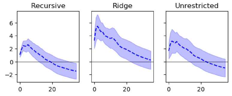
Figure 1: Oil price response to a one standard deviation oil supply shock.

Note: Symmetric $68$% bootstrap confidence bands based on $1000$ replications.

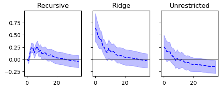
Figure 2: Oil supply response to a one standard deviation oil-specific demand shock.

Note: Symmetric $68$% bootstrap confidence bands based on $1000$ replications.

Figure 3 presents the estimated response of the oil price to stock market information shocks. All models suggest that the stock market information shock leads to an immediate increase in the stock price of around three percent and a medium-run increase in oil supply and economic activity, as documented in the appendix. This suggests that the stock market information shock contains news about future economic activity in all models. The ridge estimator and the unrestricted estimator allow to disentangle the simultaneous movement of residual oil and stock prices into oil-specific demand and stock market information shocks, which can affect both variables simultaneously. Both estimators find that the oil price immediately increases in response to the stock market information shock. In contrast, in the recursive model, the response of the oil price to stock market information shocks is restricted to zero on impact and the recursive model suggests that the information shock has no significant impact on the oil price in the medium and long run. In the recursive model, a shock that simultaneously affects the residual oil price unexplained by supply and economic activity shocks is by construction identified as an oil-specific demand shock. Therefore, information shocks which affect the oil price will be contained in the oil-specific demand shock of the recursive model, while the stock market information shock in the recursive model contains a mixture of demand and information shocks with no immediate impact on the oil price.

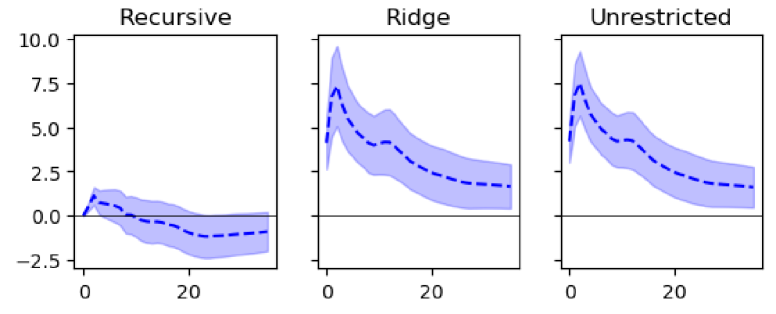
Figure 3: Oil price response to a one standard deviation stock market news shock.

Note: Symmetric $68$% bootstrap confidence bands based on $1000$ replications.

Table 2 shows the effect of the recursiveness restrictions on the forecast error variance decomposition of the oil price. According to the recursive model, oil-specific demand shocks are the primary driver, explaining more than $80$% of the variation, while supply shocks account for less than $6$% and stock market information shocks even less. In contrast, the ridge estimator suggests that oil supply and oil-specific demand both explain around $20-30$% of the oil price variation each. Therefore, the importance of supply shocks for the oil price variation is in line with the results in Baumeister and Hamilton, (2019). Moreover, the ridge estimator allows to disentangle oil-specific demand and stock market information shocks which simultaneously affect stock and oil prices. Allowing both shocks to affect the oil price simultaneously results in a larger importance of stock market information shocks, which now explain around $30-40$% of the oil price variation.

Table 2: Forecast error variance decomposition of the real price of oil.

Recursive estimator						Ridge estimator
horizon	$\varepsilon_{S}$	$\varepsilon_{Y}$	$\varepsilon_{D}$	$\varepsilon_{SM}$		horizon	$\varepsilon_{S}$	$\varepsilon_{Y}$	$\varepsilon_{D}$	$\varepsilon_{SM}$
$4$	$\underset{0.02/0.08}{0.04}$	$\underset{0.02/0.07}{0.04}$	$\underset{0.86/0.93}{0.91}$	$\underset{0.0/0.02}{0.01}$		$4$	$\underset{0.17/0.54}{0.25}$	$\underset{0.03/0.09}{0.06}$	$\underset{0.1/0.34}{0.27}$	$\underset{0.18/0.54}{0.42}$
$12$	$\underset{0.03/0.11}{0.06}$	$\underset{0.05/0.16}{0.1}$	$\underset{0.74/0.87}{0.84}$	$\underset{0.01/0.03}{0.0}$		$12$	$\underset{0.18/0.53}{0.26}$	$\underset{0.06/0.18}{0.12}$	$\underset{0.07/0.32}{0.24}$	$\underset{0.15/0.49}{0.38}$
$24$	$\underset{0.03/0.1}{0.04}$	$\underset{0.05/0.15}{0.09}$	$\underset{0.73/0.87}{0.86}$	$\underset{0.01/0.06}{0.01}$		$24$	$\underset{0.14/0.51}{0.23}$	$\underset{0.05/0.18}{0.12}$	$\underset{0.1/0.4}{0.32}$	$\underset{0.13/0.46}{0.34}$

Note: The table shows the estimated contribution of each shock to the forecast error variance decomposition of the real price of oil at $4$, $12$, and $24$ month horizon together with $68$% bootstrap confidence bands.

Figure 4 presents the historical decomposition of the oil price and sheds light on the importance of supply, demand, and information shocks in different periods. In the recursive SVAR, the oil price is predominately driven by oil-specific demand shocks, as seen in the oil price movements during significant events such as the collapse of OPEC in $1985$, the Persian Gulf War in $1990$, the oil price run up in $2007-2008$, the oil price decline and recovery following the collapse of Lehman Brothers in $2008$, the oil price decline in $2014-2016$, the oil price collapse and recovery at the beginning of the COVID-$19$ pandemic, and the recent oil price increase in $2022$ following the invasion of Ukraine.

On the other hand, the ridge estimator provides are more nuanced picture. Firstly, it suggests that supply shocks played a larger role during the collapse of OPEC in $1985$, the Persian Gulf War in $1990$, and the oil price run up in $2007-2008$. Secondly, the ridge estimator suggests that information shocks extracted from stock prices contributed largely to the oil price increase in $2007-2008$, the oil price decrease following the collapse of Lehman Brothers in $2008$, the oil price decrease in $2014-2016$, and also to the oil price decrease and recovery at the beginning of the COVID-$19$ pandemic.

Figure 4: Historical decomposition of the real oil price.

Note: Red [blue] shows the decomposition for the recursive [ridge] estimator and grey shows the historical real oil price. The vertical bars indicate the following events: Iran Iraq War ($1980:9$), collapse of OPEC ($1985:12$), Persian Gulf War ($1990:8$), the collapse of Lehman Brothers ($2008:9$), the oil price decline in mid $2014$, the beginning of the COVID-19 pandemic ($2019:3$), and the invasion of the Ukraine ($2022:3$).

Overall, the analysis suggests that the oil price responds immediately to information shocks extracted from stock prices and that these information shocks contributed largely to the oil price variation. Furthermore, including stock market information non-recursively reveals that a considerable portion of what is typically classified as oil-specific demand shocks can actually be attributed to information shocks. This finding underscores the importance of considering stock market information when examining oil price fluctuations, as it provides valuable insights into the underlying factors driving the market.

6 Conclusion

This study demonstrates the value of prior economic knowledge in combination with statistical identification approaches for SVAR models. The estimator proposed in this study uses a data-driven approach which only requires mean independent shocks to ensure identification and adds a ridge penalty to include restrictions representing uncertain prior economic knowledge. The simulations show that incorporating uncertain prior economic knowledge can enhance the accuracy of estimates and that the estimator can detect and reduce the impact of incorrect restrictions as sample size increases. The application illustrates the usefulness of the proposed estimator and highlights the role of stock market information in explaining oil price fluctuations.

Appendix A Appendix - Proof

Proof of Proposition 1.

If $B\in\mathbb{B}$ satisfies the constraint $J(B,u)$

$$E\left[e(B)_{t}e(B)^{\prime}_{t}\right]=I,$$ (16)

the objective function

$$Q(B,u):= -\sum_{i=1}^{n}\left(E[e(B)_{it}^{3}]\right)^{2}-\sum_{i=1}^{n}\left(E[e(B)_{it}^{4}-3]\right)^{2}$$

$$-6\sum_{i=1}^{n}\sum_{i=j+1}^{n}\left(E[e(B)_{it}^{2}e(B)_{jt}^{2}-1]\right)^{2}$$ (17)

is equal to

$$Q(B,u) =\omega$$ (18)

$$+3\sum_{i=1}^{n}\sum_{j=1;j\neq i}^{n}E[e(B)_{it}^{2}e(B)_{jt}]^{2}$$

$$+6\sum_{i=1}^{n}\sum_{j=i+1}^{n}\sum_{k=j+1}^{n}E[e(B)_{it}e(B)_{jt}e(B)_{kt}]^{2}$$

$$+4\sum_{i=1}^{n}\sum_{j=1;j\neq i}^{n}E[e(B)_{it}^{3}e(B)_{jt}]^{2}$$

$$+12\sum_{i=1}^{n}\sum_{j=1;j\neq i}^{n}\sum_{k=j+1;k\neq i}^{n}E[e(B)_{it}^{2}e(B)_{jt}e(B)_{kt}]^{2}$$

$$+24\sum_{i=1}^{n}\sum_{j=i+1}^{n}\sum_{k=j+1}^{n}\sum_{l=k+1}^{n}E[e(B)_{it}e(B)_{jt}e(B)_{kt}e(B)_{lt}]^{2},$$

where $\omega$ is a scalar invariant with respect to $B$ satisfying Equation (16), see Comon, (1994).

If $B$ minimizes $Q(B,u)$ under the constraint $J(B,u)$, the $B$ matrix satisfies the moment conditions

$$E[e(B)_{it}^{2}e(B)_{jt}] =0, \text{for }i \neq j$$ (19)

$$E[e(B)_{it}e(B)_{jt}e(B)_{kt}] =0, \text{for }i <j<k$$ (20)

$$E[e(B)_{it}^{3}e(B)_{jt}] =0, \text{for }i \neq j$$ (21)

$$E[e(B)_{it}^{2}e(B)_{jt}e(B)_{kt}] =0, \text{for }i \neq j,i\neq k,j<k$$ (22)

$$E[e(B)_{it}e(B)_{jt}e(B)_{kt}e(B)_{lt}] =0, \text{for }i <j<k<l.$$ (23)

The conditions hold if the shocks are mean independent or independent.

If $B$ satisfies the constraint $J(B,u)$ and Equations (19) - (20), it holds that

$$E[u_{it}u_{jt}u_{kt}]=\sum_{l=1}^{n}b_{il}b_{jl}b_{kl}E[e(B)_{lt}^{3}] \text{, for }i,j,k=1,...,n.\$$ (24)

Therefore, if at most one component of the structural shocks has zero skewness, Theorem $4$ $(ii)$ in Bonhomme and Robin, (2009) implies global identification up to sign and permutation.

Moreover, for independent shocks with at most shock exhibiting zero excess kurtosis, local identification is ensured by the asymmetric cokurtosis conditions in Equation (21), see Lanne and Luoto, (2021). However, note that even though it is not stated in the proposition in Lanne and Luoto, (2021), the proof of the proposition in Lanne and Luoto, (2021) uses the assumption that all cokurtosis conditions implied by independent shocks hold, including symmetric conditions of the type $E[e(B)_{it}^{2}e(B)_{jt}^{2}]=1$. Therefore, the proposition in Lanne and Luoto, (2021) does not ensure identification under the weaker assumption of mean independent shocks. ∎

Appendix B Appendix - Application

This section contains supplementary material for the application including several robustness checks.

Table 3 - 6 show the skewness, kurtosis, and the p-value of the Jarque-Bera test of the estimated reduced form shocks, the estimated structural shocks from the recursive estimator, the estimated structural shocks from the ridge estimator, and the estimated structural form shocks from the unrestricted estimator. The tables show that all estimated shocks are non-Gaussian, i.e. the shocks are left skewed with heavy tails.

Table 3: Skewness, kurtosis, and the p-value of the Jarque-Bera test of the estimated reduced form shocks

	$u_{q,t}$	$u_{y,t}$	$u_{p,t}$	$u_{s,t}$
Skewness	$-1.249$	$-1.596$	$-0.229$	$-1.183$
Kurtosis	$10.108$	$19.084$	$6.6$	$8.757$
JB-Test	$0$	$0$	$0$	$0$

Table 4: Skewness, kurtosis and the p-value of the Jarque-Bera test of the estimated structural shocks (recursive estimator)

	$\varepsilon_{S,t}$	$\varepsilon_{Y,t}$	$\varepsilon_{D,t}$	$\varepsilon_{SM,t}$
Skewness	$-1.249$	$-1.612$	$-0.38$	$-0.966$
Kurtosis	$10.108$	$19.091$	$5.794$	$7.365$
JB-Test	$0$	$0$	$0$	$0$

Table 5: Skewness, kurtosis and the p-value of the Jarque-Bera test of the estimated structural shocks (ridge estimator)

	$\varepsilon_{S,t}$	$\varepsilon_{Y,t}$	$\varepsilon_{D,t}$	$\varepsilon_{SM,t}$
Skewness	$-1.323$	$-1.649$	$-0.136$	$-1.52$
Kurtosis	$9.671$	$19.482$	$3.538$	$11.976$
JB-Test	$0$	$0$	$0$	$0$

Table 6: Skewness, kurtosis and the p-value of the Jarque-Bera test of the estimated structural shocks (unrestricted estimator)

	$\varepsilon_{S,t}$	$\varepsilon_{Y,t}$	$\varepsilon_{D,t}$	$\varepsilon_{SM,t}$
Skewness	$-1.36$	$-1.692$	$-0.081$	$-1.5$
Kurtosis	$10.349$	$19.763$	$3.954$	$12.173$
JB-Test	$0$	$0$	$0$	$0$

Figure 5 shows the median, $40$%, and $60$% quantiles of the loss in the let-out fold of the cross-validation for the ridge estimator. The tuning parameter is chosen analogous to the cross-validation used in the Monte Carlo simulation.

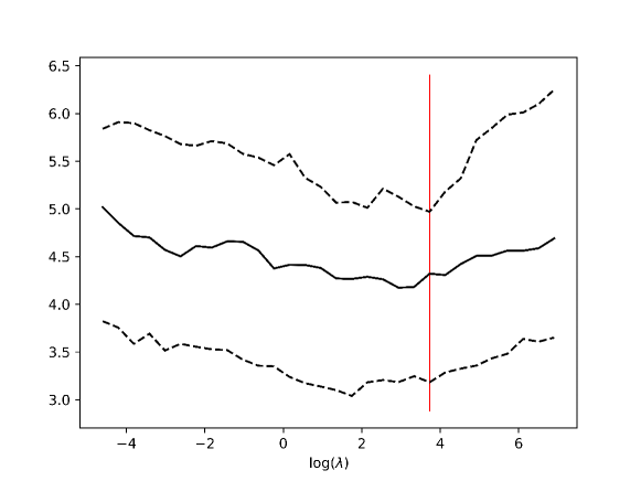
Figure 5: Median, $40$%, and $60$% quantiles of the loss in the let-out fold in a repeated cross-validation with $100$ repetitions and two folds (ridge estimator).

Figure 6, 7, 8 show the estimated impulse response for the recursive, ridge, and unrestricted estimator respectively.

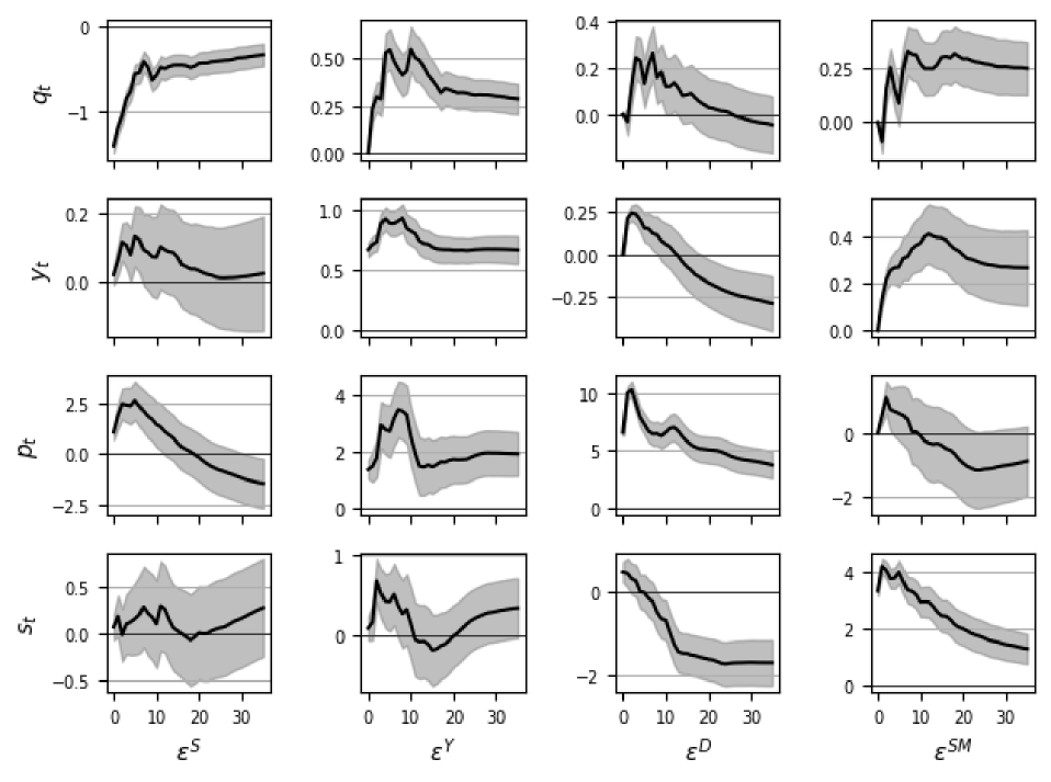
Figure 6: Impulse responses to one standard deviation shocks (recursive estimator).

Note: Symmetric $68$% bootstrap confidence bands based on $1000$ replications.

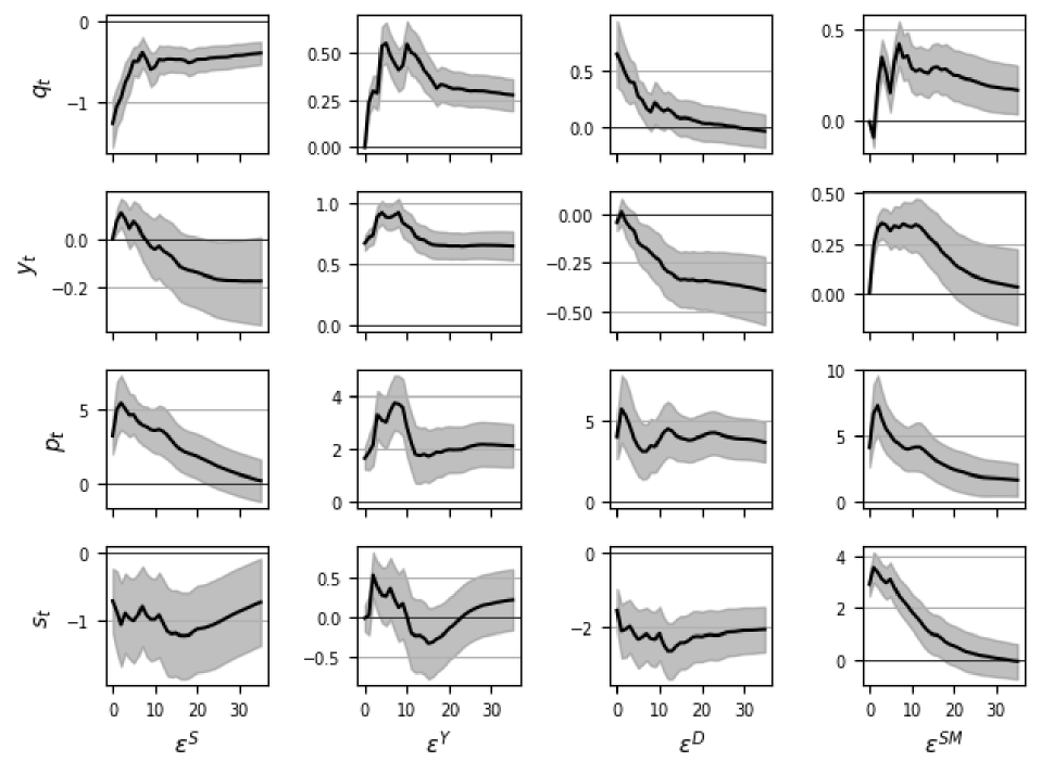
Figure 7: Impulse responses to one standard deviation shocks (ridge estimator).

Note: Symmetric $68$% bootstrap confidence bands based on $1000$ replications.

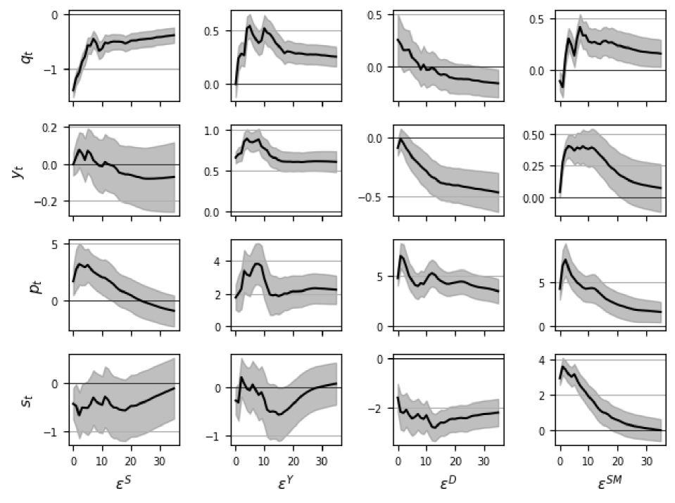
Figure 8: Impulse responses to one standard deviation shocks (unrestricted estimator).

Note: Symmetric $68$% bootstrap confidence bands based on $1000$ replications.

Figure 9 - 12 and Table 7 - 10 show that the main findings from Section 5 are robust to various modifications of the baseline specification. Specifically, all specifications find an immediate positive response of the oil price to information shocks and information shocks explain a sizable fraction of the oil price variation. Figure 9 and Table 7 show the results for a specification where the log real stock price is replaced by monthly real stock returns. Figure 10 and Table 8 show the results for a specification with $24$ lags. Figure 11 and Table 9 show the results for a specification where log industrial production is replaced by the deviation of log industrial production from a linear time trend. Figure 12 and Table 10 show the results for a specification where the log real stock price is replaced by the economic activity index based on shipping cost that was used in Kilian and Park, (2009). In this specification, the information shock is derived from the shipping index instead of the stock market.

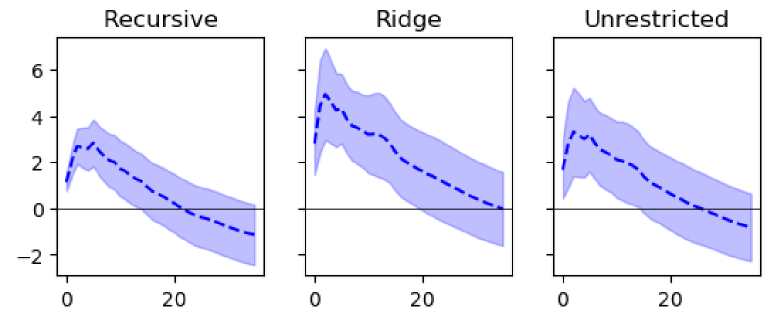
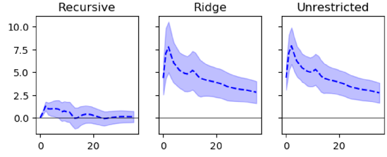
Figure 9: Oil price response to i) a one standard deviation oil supply shock (first row) and ii) to a one standard deviation stock market information shock (second row) - Specification with monthly stock returns.

Note: Symmetric $68$% bootstrap confidence bands based on $1000$ replications. This specification includes monthly real stock returns instead of log real stock prices.

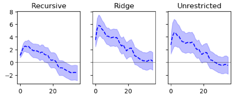
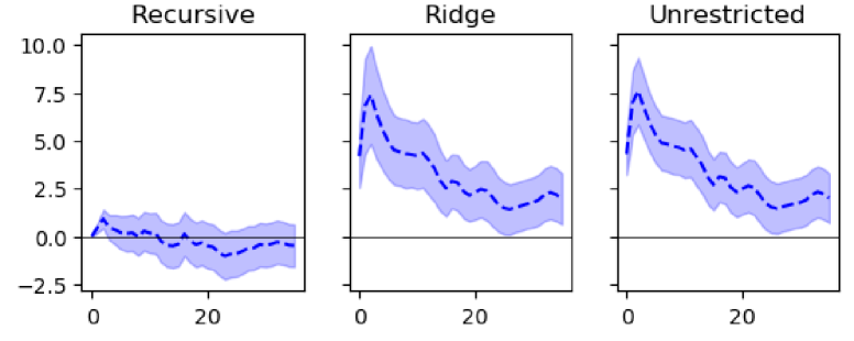
Figure 10: Oil price response to i) a one standard deviation oil supply shock (first row) and ii) to a one standard deviation stock market information shock (second row) - Specification with $24$ lags.

Note: Symmetric $68$% bootstrap confidence bands based on $1000$ replications. This specification includes $24$ lags.

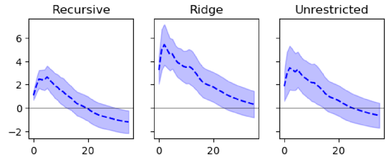
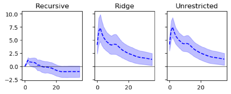
Figure 11: Oil price response to i) a one standard deviation oil supply shock (first row) and ii) to a one standard deviation stock market information shock (second row) - Specification with output gap.

Note: Symmetric $68$% bootstrap confidence bands based on $1000$ replications. This specification includes the deviation of log industrial production from a linear time trend instead of log industrial production.

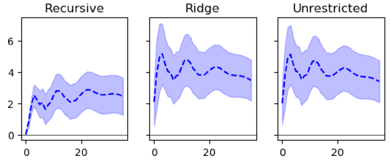
Figure 12: Oil price response to i) a one standard deviation oil supply shock (first row) and ii) to a one standard deviation dry cargo shipping information shock (second row) - Specification with the dry cargo shipping index.

Note: Symmetric $68$% bootstrap confidence bands based on $1000$ replications. This specification includes the economic activity index based on shipping cost used in Kilian and Park, (2009) instead of log real stock prices.

Table 7: FEVD of the real price of oil - Specification with monthly stock returns.

Recursive estimator						Ridge estimator
horizon	$\varepsilon_{S}$	$\varepsilon_{Y}$	$\varepsilon_{D}$	$\varepsilon_{SM}$		horizon	$\varepsilon_{S}$	$\varepsilon_{Y}$	$\varepsilon_{D}$	$\varepsilon_{SM}$
$4$	$\underset{0.03/0.08}{0.05}$	$\underset{0.02/0.07}{0.05}$	$\underset{0.84/0.93}{0.89}$	$\underset{0.0/0.02}{0.01}$		$4$	$\underset{0.12/0.49}{0.2}$	$\underset{0.03/0.09}{0.06}$	$\underset{0.08/0.34}{0.27}$	$\underset{0.19/0.6}{0.47}$
$12$	$\underset{0.03/0.12}{0.07}$	$\underset{0.06/0.16}{0.1}$	$\underset{0.73/0.87}{0.82}$	$\underset{0.0/0.03}{0.01}$		$12$	$\underset{0.13/0.49}{0.21}$	$\underset{0.06/0.17}{0.12}$	$\underset{0.06/0.31}{0.22}$	$\underset{0.17/0.57}{0.45}$
$24$	$\underset{0.03/0.11}{0.05}$	$\underset{0.04/0.15}{0.09}$	$\underset{0.74/0.88}{0.85}$	$\underset{0.01/0.04}{0.01}$		$24$	$\underset{0.1/0.48}{0.18}$	$\underset{0.05/0.17}{0.11}$	$\underset{0.08/0.37}{0.27}$	$\underset{0.16/0.56}{0.45}$

Note: The table shows the estimated contribution of each shock to the forecast error variance decomposition of the real price of oil at $4$, $12$, and $24$ month horizon together with $68$% bootstrap confidence bands. This specification includes monthly real stock returns instead of log real stock prices.

Table 8: FEVD of the real price of oil - Specification with $24$ lags.

Recursive estimator						Ridge estimator
horizon	$\varepsilon_{S}$	$\varepsilon_{Y}$	$\varepsilon_{D}$	$\varepsilon_{SM}$		horizon	$\varepsilon_{S}$	$\varepsilon_{Y}$	$\varepsilon_{D}$	$\varepsilon_{SM}$
$4$	$\underset{0.02/0.08}{0.05}$	$\underset{0.03/0.1}{0.06}$	$\underset{0.84/0.92}{0.89}$	$\underset{0.0/0.01}{0.0}$		$4$	$\underset{0.22/0.63}{0.3}$	$\underset{0.04/0.1}{0.06}$	$\underset{0.07/0.28}{0.19}$	$\underset{0.08/0.55}{0.45}$
$12$	$\underset{0.03/0.12}{0.06}$	$\underset{0.08/0.22}{0.14}$	$\underset{0.68/0.85}{0.8}$	$\underset{0.0/0.03}{0.0}$		$12$	$\underset{0.22/0.61}{0.31}$	$\underset{0.08/0.22}{0.14}$	$\underset{0.05/0.25}{0.16}$	$\underset{0.07/0.49}{0.39}$
$24$	$\underset{0.03/0.13}{0.05}$	$\underset{0.08/0.24}{0.16}$	$\underset{0.63/0.82}{0.79}$	$\underset{0.01/0.05}{0.0}$		$24$	$\underset{0.2/0.59}{0.3}$	$\underset{0.08/0.25}{0.16}$	$\underset{0.06/0.29}{0.18}$	$\underset{0.07/0.47}{0.36}$

Note: The table shows the estimated contribution of each shock to the forecast error variance decomposition of the real price of oil at $4$, $12$, and $24$ month horizon together with $68$% bootstrap confidence bands. This specification includes $24$ lags.

Table 9: FEVD of the real price of oil - Specification with output gap.

Recursive estimator						Ridge estimator
horizon	$\varepsilon_{S}$	$\varepsilon_{Y}$	$\varepsilon_{D}$	$\varepsilon_{SM}$		horizon	$\varepsilon_{S}$	$\varepsilon_{Y}$	$\varepsilon_{D}$	$\varepsilon_{SM}$
$4$	$\underset{0.02/0.08}{0.05}$	$\underset{0.02/0.07}{0.05}$	$\underset{0.85/0.93}{0.9}$	$\underset{0.0/0.02}{0.01}$		$4$	$\underset{0.19/0.52}{0.24}$	$\underset{0.03/0.09}{0.06}$	$\underset{0.11/0.34}{0.27}$	$\underset{0.17/0.51}{0.42}$
$12$	$\underset{0.03/0.11}{0.06}$	$\underset{0.06/0.17}{0.12}$	$\underset{0.72/0.87}{0.82}$	$\underset{0.01/0.03}{0.01}$		$12$	$\underset{0.19/0.52}{0.25}$	$\underset{0.07/0.19}{0.14}$	$\underset{0.08/0.31}{0.23}$	$\underset{0.15/0.47}{0.38}$
$24$	$\underset{0.03/0.1}{0.04}$	$\underset{0.06/0.2}{0.12}$	$\underset{0.69/0.86}{0.83}$	$\underset{0.01/0.05}{0.01}$		$24$	$\underset{0.15/0.48}{0.22}$	$\underset{0.07/0.23}{0.15}$	$\underset{0.09/0.37}{0.29}$	$\underset{0.12/0.45}{0.34}$

Note: The table shows the estimated contribution of each shock to the forecast error variance decomposition of the real price of oil at $4$, $12$, and $24$ month horizon together with $68$% bootstrap confidence bands. This specification includes the deviation of log industrial production from a linear time trend instead of log industrial production.

Table 10: FEVD of the real price of oil - Specification with the dry cargo shipping index.

Recursive estimator						Ridge estimator
horizon	$\varepsilon_{S}$	$\varepsilon_{Y}$	$\varepsilon_{D}$	$\varepsilon_{SM}$		horizon	$\varepsilon_{S}$	$\varepsilon_{Y}$	$\varepsilon_{D}$	$\varepsilon_{SM}$
$4$	$\underset{0.02/0.07}{0.04}$	$\underset{0.03/0.08}{0.05}$	$\underset{0.83/0.91}{0.88}$	$\underset{0.02/0.05}{0.03}$		$4$	$\underset{0.04/0.6}{0.15}$	$\underset{0.03/0.1}{0.07}$	$\underset{0.21/0.63}{0.58}$	$\underset{0.04/0.3}{0.2}$
$12$	$\underset{0.03/0.11}{0.06}$	$\underset{0.06/0.17}{0.11}$	$\underset{0.68/0.82}{0.78}$	$\underset{0.03/0.1}{0.06}$		$12$	$\underset{0.06/0.58}{0.16}$	$\underset{0.07/0.19}{0.14}$	$\underset{0.15/0.52}{0.46}$	$\underset{0.06/0.35}{0.25}$
$24$	$\underset{0.03/0.1}{0.04}$	$\underset{0.05/0.15}{0.09}$	$\underset{0.64/0.81}{0.78}$	$\underset{0.04/0.18}{0.09}$		$24$	$\underset{0.05/0.53}{0.12}$	$\underset{0.05/0.18}{0.12}$	$\underset{0.15/0.51}{0.45}$	$\underset{0.08/0.43}{0.31}$

Note: The table shows the estimated contribution of each shock to the forecast error variance decomposition of the real price of oil at $4$, $12$, and $24$ month horizon together with $68$% bootstrap confidence bands. This specification includes the economic activity index based on shipping cost used in Kilian and Park, (2009) instead of log real stock prices.

References

- Abhyankar et al., (2013) Abhyankar, A., Xu, B., and Wang, J. (2013). Oil price shocks and the stock market: evidence from japan. The Energy Journal, 34(2).
- Ahmadi et al., (2016) Ahmadi, M., Manera, M., and Sadeghzadeh, M. (2016). Global oil market and the us stock returns. Energy, 114:1277–1287.
- Anttonen et al., (2021) Anttonen, J., Lanne, M., and Luoto, J. (2021). Statistically Identified SVAR Model with Potentially Skewed and Fat-Tailed Errors. Available at SSRN 3925575.
- Apergis and Miller, (2009) Apergis, N. and Miller, S. M. (2009). Do Structural Oil-Market Shocks Affect Stock Prices? Energy Economics, 31(4):569–575.
- Arampatzidis et al., (2021) Arampatzidis, I., Dergiades, T., Kaufmann, R. K., and Panagiotidis, T. (2021). Oil and the us stock market: Implications for low carbon policies. Energy Economics, 103:105588.
- Baumeister and Hamilton, (2019) Baumeister, C. and Hamilton, J. D. (2019). Structural Interpretation of Vector Autoregressions with Incomplete Identification: Revisiting the Role of Oil Supply and Demand Shocks. American Economic Review, 109(5):1873–1910.
- Baumeister and Hamilton, (2022) Baumeister, C. and Hamilton, J. D. (2022). Structural vector autoregressions with imperfect identifying information. In AEA Papers and Proceedings, volume 112, pages 466–70.
- Baumeister et al., (2022) Baumeister, C., Korobilis, D., and Lee, T. K. (2022). Energy markets and global economic conditions. Review of Economics and Statistics, 104(4):828–844.
- Bertsche and Braun, (2022) Bertsche, D. and Braun, R. (2022). Identification of structural vector autoregressions by stochastic volatility. Journal of Business & Economic Statistics, 40(1):328–341.
- Blanchard and Quah, (1989) Blanchard, O. J. and Quah, D. (1989). The Dynamic Effects of Aggregate Demand and Supply Disturbances. The American Economic Review, 79(4):655–673.
- Bonhomme and Robin, (2009) Bonhomme, S. and Robin, J.-M. (2009). Consistent Noisy Independent Component Analysis. Journal of Econometrics, 149(1):12–25.
- Braun, (2021) Braun, R. (2021). The importance of supply and demand for oil prices: evidence from non-gaussianity.
- Caldara et al., (2019) Caldara, D., Cavallo, M., and Iacoviello, M. (2019). Oil price elasticities and oil price fluctuations. Journal of Monetary Economics, 103:1–20.
- Comon, (1994) Comon, P. (1994). Independent Component Analysis, a New Concept? Signal processing, 36(3):287–314.
- Dai et al., (2018) Dai, L., Chen, K., Sun, Z., Liu, Z., and Li, G. (2018). Broken adaptive ridge regression and its asymptotic properties. Journal of multivariate analysis, 168:334–351.
- Frommlet and Nuel, (2016) Frommlet, F. and Nuel, G. (2016). An adaptive ridge procedure for l 0 regularization. PloS one, 11(2):e0148620.
- Gouriéroux et al., (2017) Gouriéroux, C., Monfort, A., and Renne, J.-P. (2017). Statistical Inference for Independent Component Analysis: Application to Structural VAR Models. Journal of Econometrics, 196(1):111–126.
- Guay, (2021) Guay, A. (2021). Identification of Structural Vector Autoregressions Through Higher Unconditional Moments. Journal of Econometrics, 225(1):27–46.
- Herwartz and Plödt, (2016) Herwartz, H. and Plödt, M. (2016). The Macroeconomic Effects of Oil Price Shocks: Evidence from a Statistical Identification Approach. Journal of International Money and Finance, 61:30–44.
- Kang and Ratti, (2013) Kang, W. and Ratti, R. A. (2013). Oil shocks, policy uncertainty and stock market return. Journal of International Financial Markets, Institutions and Money, 26:305–318.
- (21) Keweloh, S. A. (2021a). A Feasible Approach to Incorporate Information in Higher Moments in Structural Vector Autoregressions. Discussion Papers SFB 823.
- (22) Keweloh, S. A. (2021b). A Generalized Method of Moments Estimator for Structural Vector Autoregressions Based on Higher Moments. Journal of Business & Economic Statistics, 39(3):772–782.
- Keweloh et al., (2023) Keweloh, S. A., Klein, M., and Prüser, J. (2023). Estimating the effects of fiscal policy using a novel proxy shrinkage prior. arXiv preprint arXiv:2302.13066.
- Kilian and Murphy, (2012) Kilian, L. and Murphy, D. P. (2012). Why agnostic sign restrictions are not enough: understanding the dynamics of oil market var models. Journal of the European Economic Association, 10(5):1166–1188.
- Kilian and Murphy, (2014) Kilian, L. and Murphy, D. P. (2014). The Role of Inventories and Speculative Trading in the Global Market for Crude Oil. Journal of Applied econometrics, 29(3):454–478.
- Kilian and Park, (2009) Kilian, L. and Park, C. (2009). The Impact of Oil Price Shocks on the US Stock Market. International Economic Review, 50(4):1267–1287.
- Kwon, (2022) Kwon, D. (2022). The impacts of oil price shocks and united states economic uncertainty on global stock markets. International Journal of Finance & Economics, 27(2):1595–1607.
- Lambertides et al., (2017) Lambertides, N., Savva, C. S., and Tsouknidis, D. A. (2017). The effects of oil price shocks on us stock order flow imbalances and stock returns. Journal of International Money and Finance, 74:137–146.
- Lanne et al., (2022) Lanne, M., Liu, K., and Luoto, J. (2022). Identifying structural vector autoregression via leptokurtic economic shocks. Journal of Business & Economic Statistics, (just-accepted):1–27.
- Lanne and Luoto, (2020) Lanne, M. and Luoto, J. (2020). Identification of Economic Shocks by Inequality Constraints in Bayesian Structural Vector Autoregression. Oxford Bulletin of Economics and Statistics, 82(2):425–452.
- Lanne and Luoto, (2021) Lanne, M. and Luoto, J. (2021). GMM Estimation of Non-Gaussian Structural Vector Autoregression. Journal of Business & Economic Statistics, 39(1):69–81.
- Lanne et al., (2010) Lanne, M., Lütkepohl, H., and Maciejowska, K. (2010). Structural Vector Autoregressions with Markov Switching. Journal of Economic Dynamics and Control, 34(2):121–131.
- Lanne et al., (2017) Lanne, M., Meitz, M., and Saikkonen, P. (2017). Identification and Estimation of Non-Gaussian Structural Vector Autoregressions. Journal of Econometrics, 196(2):288–304.
- Lewis, (2021) Lewis, D. J. (2021). Identifying Shocks via Time-Varying Volatility. The Review of Economic Studies, 88(6):3086–3124.
- Lütkepohl and Netšunajev, (2017) Lütkepohl, H. and Netšunajev, A. (2017). Structural Vector Autoregressions with Smooth Transition in Variances. Journal of Economic Dynamics and Control, 84:43–57.
- Matteson and Tsay, (2017) Matteson, D. S. and Tsay, R. S. (2017). Independent component analysis via distance covariance. Journal of the American Statistical Association, 112(518):623–637.
- Mertens and Ravn, (2013) Mertens, K. and Ravn, M. O. (2013). The Dynamic Effects of Personal and Corporate Income Tax Changes in the United States. American Economic Review, 103(4):1212–47.
- Mokni, (2020) Mokni, K. (2020). Time-varying effect of oil price shocks on the stock market returns: Evidence from oil-importing and oil-exporting countries. Energy Reports, 6:605–619.
- Montiel Olea et al., (2022) Montiel Olea, J. L., Plagborg-Møller, M., and Qian, E. (2022). Svar identification from higher moments: Has the simultaneous causality problem been solved? In AEA Papers and Proceedings, volume 112, pages 481–85.
- Rigobon, (2003) Rigobon, R. (2003). Identification through Heteroskedasticity. Review of Economics and Statistics, 85(4):777–792.
- Sim and Zhou, (2015) Sim, N. and Zhou, H. (2015). Oil prices, us stock return, and the dependence between their quantiles. Journal of Banking & Finance, 55:1–8.
- Sims, (1980) Sims, C. A. (1980). Macroeconomics and Reality. Econometrica: Journal of the Econometric Society, pages 1–48.
- Uhlig, (2005) Uhlig, H. (2005). What are the Effects of Monetary Policy on Output? Results from an Agnostic Identification Procedure. Journal of Monetary Economics, 52(2):381–419.
- Zou, (2006) Zou, H. (2006). The adaptive lasso and its oracle properties. Journal of the American statistical association, 101(476):1418–1429.