cram rectangle=false, cram width=2.5pt, cram dash width=0.4pt, cram dash sep=1pt, atom sep=16pt, bond offset=1pt, double bond sep=2pt

Parameterized Algorithms for Topological Indices in Chemistry

Abstract: We have developed efficient parameterized algorithms for the enumeration problems of graphs arising in chemistry. In particular, we have focused on the following problems: enumeration of Kekulé structures, computation of Hosoya index, computation of Merrifield–Simmons index, and computation of graph entropy based on matchings and independent sets. All these problems are known to be $\#P$-complete. We have developed FPT algorithms for bounded treewidth and bounded pathwidth for these problems with a better time complexity than the known state-of-the-art in the literature. We have also conducted experiments on the entire PubChem database of chemical compounds and tested our algorithms. We also provide a comparison with naive baseline algorithms for these problems, along with a distribution of treewidth for the chemical compounds available in the PubChem database.

Keywords: Computational Chemistry, Parameterized Algorithms, Topological Indices.

Acknowledgment: The research was partially supported by the Hong Kong RGC ECS Project 26208122, the HKUST-Kaisa Grant HKJRI3A-055, the HKUST Startup Grant R9272, UGent Grant BOF21/DOC/182 and the Sofina-Boël Fellowship Program. Authors are ordered alphabetically.

1 Introduction

1.1 Enumeration problems in chemistry

We studied the enumeration problems on the molecular graphs in chemistry. We focused on the following problems:

• Enumeration of Kekulé structures - The Kekulé structure for a molecule is essentially a perfect matching of the underlying graph. Therefore, enumeration of Kekulé structures is equal to computing total number of perfect matchings of the graph [Tri18].

• Hosoya index - The Hosoya index, also known as Z index, of a graph is the total number of matchings of the graph [Hos71].

• Merrifield–Simmons index - The Merrifield–Simmons index of a graph is the total number of independent sets of the graph [MS80].

• Graph entropy based on matchings and independent sets - The computation of graph entropy based on matchings and independent sets is equivalent to determining all matchings and independent sets for every possible size [CDK17].

All these problems are known to be $\#P$-complete. The existing theoretical results for these problems are not useful for real-world applications in chemistry where graphs may have a large number of vertices and edges.

1.2 Importance

Topological indices are numerical graph invariants that characterizes the topology of graph [Tri18]. These indices play a vital role in computational chemistry. In particular, they are used as molecular descriptors for QSAR (Quantitative structure-activity relationship) and QSPR (Quantitative structure property relationships) [Dea17]. In other words, the topology of hydrogen-supressed graphs of molecule can be used to quantitatively describe the physical and chemical properties. The problems under considerations are some of the well studied examples of molecular descriptors over the years in chemistry literature.

1.3 Our contribution

We provide new algorithms for the above mentioned problems that works in polynomial time for graphs that have small treewidth and small pathwidth. We can handle more than $99.9\%$ of molecules in the PubChem database. Moreover, we also provide a statistical distribution of treewidth for the entire PubChem database [KCC⁺23]. Hence, we think this result would serve as an invitaion to both chemists and computer scientists to use parameterized algorithms more often for the problems arising in computional chemistry and biology.

1.3.1 Parameterized Algorithms

An efficient parameterized algorithm solves a problem in polynomial time with respect to the size of input, but possibly with non-polynomial dependence on a specific aspect of the input’s structure, which is called a “parameter”. A problem that can be solved by an efficient parameterized algorithm is called fixed-parameter tractable (FPT).

1.3.2 Pathwidth and Treewidth

Pathwidth and treewidth are well studied parameters for graphs. Informally, pathwidth is the measure of path-likeness of a graph and treewidth is a measure of tree-likeness of a graph. Many hard graph problems in computer science are shown to have efficient solutions when restricted to graphs with bounded treewidth and bounded pathwidth. In this work we show that more than $99.9\%$ molecules in the enitre PubChem database have treewidht less than $5$, less than $100$ molecules have treewidth greater than $20$, in the enitre database of more than $100$ million compounds. For more detailed statistics for the entire database refer to Section 4. Therefore, supporting our argument of developing parameterized algorithms for bounded treewidth and pathwidth for the above mentioned problems.

1.4 Related works

• In theory, there are known FPT algorithms using bounded treewidth as parameter for computing matchings and independent using monadic second order logic [CMR01]. But it is impractical to implement and use them for graphs with large number of vertices and edges arising in chemistry.

• In [WTZL18], the authors have provided explicit parameterized algorihtms for computing graph entropies corresponding to Hosoya Index and Merrifield–Simmons Index. But our algorithms, are better than their approach by a linear factor for computing the graph entropies and by a quadratic factor for computing the corresponding indices. We also provide a practical implementaion for all the graphs obtained from PubChem database.

1.5 Structure of the paper

The paper is divided into three main sections. We first start with basic notations and preliminaries in Section 2. Our main algorithms and theoretical reults are described in Section 3. We provide all the experimental results, statistics and implementation details in Section 4. Finally, we end the paper with conclusion in Section 5.

2 Notations and Preliminaries

2.1 Basic definitions

Definition 1 (Path Decomposition [CFK⁺15]).

A path decomposition of a graph $G=(V,E)$ is a sequence of bags $\mathcal{P}=\{X_{1},\dots,X_{r}\}$, where each $X_{i}\subseteq V$ such that following conditions hold:

1. For each $v\in V$, there exists a pair of indices $1\leq l(v)\leq r(v)\leq r$ such that

   $$v\in X_{i}\Longleftrightarrow l(v)\leq i\leq r(v).$$

   In other words each graph vertex maps to continuous subpath of the decomposition.

2. For each $uv\in E$, there exists an $i$ such that $\{u,v\}\subseteq X_{i}$.

Definition 2 (Nice Path Decomposition [CFK⁺15]).

A nice path decomposition is a path decomposition, where additional conditions hold:

1. $X_{1},X_{r}=\varnothing$.

2. Each bag, except $X_{1}$, either introduce or forget node.

3. If $X_{i+1}$ is a forget node, then there exists $v\in V$ such that $X_{i+1}=X_{i}\setminus\{v\}$.

4. If $X_{i+1}$ is an introduce node, then there exists $v\in V$ such that $X_{i+1}=X_{i}\cup\{v\}$.

Definition 3 (Pathwidth [CFK⁺15]).

The width of a path decomposition $\mathcal{P}=\{X_{1},\dots,X_{r}\}$ is $max_{1\leq i\leq r}\lvert X_{i}\rvert-1$. The pathwidth of a graph $G$, denoted by pw(G), is the minimum possible width of a path decomposition of G.

Definition 4 (Tree Decomposition [CFK⁺15]).

A tree decomposition of a graph $G$ is a pair $\mathcal{T}=(T,\{X_{t}\}_{t\in V(T)})$, where $T$ is a rooted tree with a root $r$, each bag $X_{t}\subseteq V(G)$ and the following conditions hold:

1. For every $uv\in E(G)$, there exists a node $t\in V(T)$ such that $\{u,v\}\subseteq X_{t}$.

2. For every $v\in V(G)$, the set $T_{v}:=\{t\in V(T):v\in X_{t}\}$, induced graph $T[T_{v}]$ is nonempty subtree of the $T$.

Definition 5 (Nice Tree Decomposition [CFK⁺15]).

A nice tree decomposition is a tree decomposition, where additional conditions hold:

1. The root bag is empty: $X_{r}=\varnothing$.

2. If $l$ is a leaf of the $T$, then $X_{l}=\varnothing$.

3. Each non-leaf node of tree $T$ is of one of the three types: introduce, forget or join node.

4. If $X_{b}$ is a forget node, it has exactly one child $X_{c}$ and there is a vertex $v\in X_{c}$ such that $X_{b}=X_{c}\setminus\{v\}$.

5. If $X_{b}$ is an introduce node, it has exactly one child $X_{c}$ and there is a vertex $v\in V(G)\setminus X_{c}$ such that $X_{b}=X_{c}\cup\{v\}$.

6. If $X_{b}$ is a join node, it has exactly two children $X_{c_{1}}$ and $X_{c_{2}}$ such that $X_{b}=X_{c_{1}}=X_{c_{2}}$.

Definition 6 (Treewidth [CFK⁺15]).

The width of tree decomposition $\mathcal{T}=(T,\{X_{t}\}_{t\in V(T)})$ equals $max_{t\in V(T)}\lvert X_{t}\rvert-1$, that is, the maximum size of its bag minus 1. The treewidth of a graph $G$, denoted by $tw(G)$, is the minimum possible width of a tree decomposition of $G$.

Remark 1.

Notice that (nice) path decomposition is a special case of a (nice) tree decomposition. For a path decomposition $\mathcal{P}=\{X_{1},\dots,X_{r}\}$ we think that the $X_{1}$ is a leaf bag and the $X_{r}$ is a root bag.

Notation 1.

For each $t\in G(T)$ we denote subtree rooted at this vertex as $T_{t}$, and denote a graph induced by all vertices in all bags correspond to $T_{t}$:

$$G^{\downarrow}_{t}:=G\left[\bigcup\{X_{t}:t\in T_{t}\}\right].$$

Example 1.

In this example, we explain the above defintions by explicitly showing tree decomposition for underlying graph of Caffeine molecule (See Figure 1).

O=[:270]-[:210]N(-[:150])-[:270](=[:210]O)-[:330]N(-[:270])-[:30]-[:342.2,0.994]N=^[:54,0.994]-[:126,0.994]N(-[:71.9])-[:197.8,0.994](=^[:270])(-[:150])

Figure 1: Caffeine

We can see from Figure 2, that Caffeine molecule has treewidth $2$.

(a)

(b)

Figure 2: Graph representation and tree decomposition of Caffeine.

2.2 Technical Lemmas

We now present two technical lemmas that are crucial for development of algorithms in Section 3. These lemmas are consequences of separation properties of the tree decomposition.

Lemma 1.

If $X_{b}$ is an introduce nodes, $X_{b}=X_{c}\cup\{v\}$, then $N(v)\cap G_{b}^{\downarrow}\subseteq X_{c}$.

Proof.

Let $T^{\prime}$ be a subtree of the tree $T$ rooted at $b$. Observe that the corresponding tree decomposition $\mathcal{T}^{\prime}=\{T^{\prime},\{X_{t}\}_{t\in V(T^{\prime})}\}$ is a tree decomposition of $G_{b}^{\downarrow}$. Notice that by Definition 4, $T^{\prime}_{v}$ forms an induced subtree of the $T^{\prime}$. As $v\notin X_{c}$ and $c$ is the only vertex in the open neighbourhood of $b$, this implies that $T^{\prime}_{v}=\{b\}$.

Let $u$ be a vertex in $N(v)\cap G_{b}^{\downarrow}$, then by Definition 4, if there is an edge $uv$ in $G_{b}^{\downarrow}$, then there exists a bag containing both $u$ and $v$. But, as we have just shown that the only bag containing $v$ is $X_{b}$. As $u$ is a vertex in $N(v)$, this implies that $u\in X_{c}$. ∎

Lemma 2.

If $X_{b}$ is a join node with two children $X_{b}=X_{c_{1}}=X_{c_{2}}$, then in $G_{b}^{\downarrow}$ there is no edge between $V(G_{c_{1}}^{\downarrow})\setminus X_{b}$ and $V(G_{c_{2}}^{\downarrow})\setminus X_{b}$.

Proof.

Let $T^{\prime},T^{\prime\prime},T^{\prime\prime\prime}$ be the subtrees of $T$ rooted at $b,c_{1},c_{2}$ respectively. Let $\mathcal{T}^{\prime},\mathcal{T}^{\prime\prime},\mathcal{T}^{\prime\prime\prime}$ be the corresponding tree decompositions. We will prove the given statement by contradiction. Therefore, let us assume that $u\in V(G_{c_{1}}^{\downarrow})\setminus X_{b}$, $v\in V(G_{c_{2}}^{\downarrow})\setminus X_{b}$, and $uv\in E(G_{b}^{\downarrow})$.

As $\mathcal{T}^{\prime}$ is a tree decomposition of $G^{\downarrow}_{b}$, there exists at least one bag $X_{t}$, such that $t\in\mathcal{T}^{\prime}$ and $u,v\in X_{t}$. From our initial assumption, we know that $u,v\notin X_{b}$, this implies that $t\neq b$. Therefore, either $t\in T^{\prime\prime}$ or $t\in T^{\prime\prime\prime}$. Without loss of generality, let us assume that $t\in T^{\prime\prime}$. As $v\in V(G_{c_{2}}^{\downarrow})\setminus X_{b}$, there exists at least one bag $X_{s}$ such that, $s\in T^{\prime\prime\prime}$ and $v\in X_{s}$. Observe that $v$ appears in both bags $X_{s}$ and $X_{t}$. Now by Definition 4, we know that $T^{\prime}_{v}$ is a connected subtree and any path connecting $s$ and $t$ goes through $b$. This implies that $X_{b}\in T^{\prime}_{v}$ and $v\in X_{b}$. This contradicts our initial assumption that $v\notin X_{b}$, hence completes the proof. ∎

3 Our Algorithms

3.1 Counting Perfect Matchings

Enumeration of Kekulé structures in organic molecules is equivalent to finding total number of perfect matchings for the underlying chemical graph of the molecule.

We present parametrized algorithms for the cases when the underlying chemical graph have bounded pathwidth and bounded treewidth respectively.

3.1.1 Bounded Pathwidth

We will use a dynamic programming approach over the nice path decomposition of the given graph $G$. First we will define the dynamic programming state as follows:

Definition 7 (Respectful Perfect Matchings).

Let us fix a nice path decomposition $\mathcal{P}=\{X_{1},\dots X_{r}\}$ for the given graph $G$. For each $b\in[r]$ and each $M\subseteq X_{b}$, we define $\mathcal{RP}(b,M)$ as the set of all perfect matchings $F$ in a $G_{b}^{\downarrow}\setminus M$ such that each matching edge $uv\in F$ has at least one point in $G_{b}^{\downarrow}\setminus X_{b}$: $u\notin X_{b}$ or $v\notin X_{b}$.

Definition 8 (Dynamic Programming State for Perfect Matchings).

Let us fix a nice path decomposition $\mathcal{P}=\{X_{1},\dots X_{r}\}$ for the given graph $G$. For each $b\in[r]$ and each $M\subseteq X_{b}$, we define $\textup{PerfMatch}[b,M]$ to be the number of elements in the set $\mathcal{RP}(b,M)$.

Remark 2.

Notice that if $X_{r}=\varnothing$ is the root node, then $G_{r}^{\downarrow}=G$, and perfect matchings of $G$ are in one-to-one correspondence with respectful perfect matchings $\mathcal{RP}(r,\varnothing)$, which implies $\textup{PerfMatch}[r,\varnothing]$ is the total number of perfect matchings of $G$.

We now provide a bottom-up approach for filling up the dynamic table. The dynamic table relations depend on the type of the bag. We need to consider three cases when $X_{b}$ is: leaf node, introduce node and forget node respectively. We refer the reader to follow proof along with Example 2 for better clarity of the dynamic programming approach.

• Leaf node: If $X_{l}$ is a leaf bag then $\mathcal{RP}(b,M)$ contains only empty matching as $X_{l}=\varnothing$. Therefore, $\textup{PerfMatch}[l,\varnothing]=1$.

• Introduce node: Let $X_{b}$ be an introduce bag such that $X_{b}=X_{c}\cup\{v\}$. Then the dynamic programming state corresponding to $(b,M)$ satisfies the following recurrence relations:

  $$\textup{PerfMatch}[b,M]=\begin{cases}\textup{PerfMatch}[c,M\setminus v],&v\in M,\\ 0,&v\not\in M.\end{cases}$$

  In order to derive the above recurrence relations, we have to consider two possibilities for $v$.

  1. If $v\in M$, then by Definition 7, all the elements of the set $\mathcal{RP}(b,M)$ are in one-to-one correspondence with all the elements of the set $\mathcal{RP}(c,M\setminus v)$.

  2. If $v\notin M$, then for every matching $F\in\mathcal{RP}(b,M)$, $v$ should be covered by some edge $vw\in F$. By Lemma 1, $w\in X_{c}\subset X_{b}$, which contradicts the Definition 7. Therefore, $\textup{PerfMatch}[b,m]=0$ for this case, as there are no matchings satisfying the given conditions.

  This transition from $X_{c}$ to $X_{b}$ can be computed in $\mathcal{O}(1)$ time.

• Forget node: Let $X_{b}$ be the forget node such that $X_{b}=X_{c}\setminus\{v\}$. Then the dynamic programming state corresponding to $(b,M)$ satisfies the following recurrence relation:

  $$\textup{PerfMatch}[b,M]=\textup{PerfMatch}[c,M]+\sum_{u\in X_{b}\setminus M:\ uv\in E(G)}\textup{PerfMatch}[c,M\cup\{v,u\}]$$

  In order to derive the above recurrence relation, let $F$ be a matching from the set $\mathcal{RP}(b,M)$. Note that $v\notin M$, as $M\subseteq X_{b}$. Therefore, $v$ will be matched by some edge $uv\in F$. Now there are two possible cases i.e., either $u\notin X_{b}$ or $u\in X_{b}$. For the former case when $u\notin X_{b}$, it is clear that there is a bijection between all such matchings $F$ and all elements of $\mathcal{RP}(c,M)$. Therefore, number of such matchings correspond to the first term $\textup{PerfMatch}[c,M]$ of the recurrence relation. Now let’s consider the latter case when $u\in X_{b}$, then the matching $F\setminus uv\in\mathcal{RP}(c,MM\cup\{u,v\})$, and number of such matchings correspond to the second term $\sum_{u\in X_{b}\setminus M:\ uv\in E(G)}\textup{PerfMatch}[c,M\cup\{v,u\}]$ of the recurrence relation.

  This transition to $X_{b}$ can be computed in $\mathcal{O}(\lvert X_{b}\rvert)=\mathcal{O}(\textup{pw}(G))$ time.

Proposition 3.

The time complexity for finding the total number of perfect matchings for a graph $G=(V,E)$, with $\lvert V\rvert=n$ and pathwidth pw, using the above algorithm is $\mathcal{O}(n\cdot\textup{poly}(\textup{pw})\cdot 2^{\textup{pw}})$.

Proof.

For each bag, we have at most $2^{\textup{pw}}$ dynamic programming states, and for each state we spend at most $\mathcal{O}(\textup{poly}(\textup{pw}))$ time. It is known that there are at most $\mathcal{O}(n\cdot\textup{pw})$ bags for any nice path decomposition of $G$ [CFK⁺15, Chapter 7]. Therefore, we spend at most $\mathcal{O}(n\cdot\textup{poly}(\textup{pw})\cdot 2^{\textup{pw}})$ time to completely fill the dymamic programming table. ∎

3.1.2 Bounded Treewidth

We will use a dynamic programming approach over the nice tree decomposition of the given graph $G$. The definitions of respectful perfect matchings and dynamic programming states used here are same as Section 3.1.1. Let $\mathcal{T}=\{T,\{X_{t}\}_{t\in V(T)}\}$ be a nice tree decomposition of the graph $G=(V,E)$ under consideration.

We now provide a bottom-up approach for filling up the dynamic table. The dynamic table relations depend on the type of the bag. There are four possible cases for the type of bags, i.e., when $X_{b}$ is: leaf node, introduce node, forget node and join node respectively. The reccurrence relations for leaf node, introduce node and forget node remains the same as Section 3.1.1. Therefore, we only need to consider the case of join node which is described as follows:

• Join node: Let $X_{b}$ be the join node with $X_{c_{1}}$ and $X_{c_{2}}$ as its children. Then the dynamic programming state corresponding to $(b,M)$ will satisfy the following recurrence relation:

  $$\textup{PerfMatch}[b,M]=\sum_{H_{1}\sqcup H_{2}=X_{b}\setminus M}\textup{PerfMatch}[c_{1},M\cup H_{2}]\cdot\textup{PerfMatch}[c_{2},M\cup H_{1}]$$

  where $H_{1}\sqcup H_{2}=X_{b}\setminus M$ means $H_{1}\cup H_{2}=X_{b}\setminus M$ and $H_{1}\cap H_{2}=\varnothing$. In order to derive the above recurrence relation, let $F$ be a matching from the set $\mathcal{RP}(b,M)$. By Lemma 2, $F$ doesn’t have any edges between $G_{c_{1}}^{\downarrow}\setminus X_{b}$ and $G_{c_{2}}^{\downarrow}\setminus X_{b}$. Therefore, it can be split into two matchings, $F_{1}:=E(G_{c_{1}}^{\downarrow})\cap F$ and $F_{2}:=E(G_{c_{2}}^{\downarrow})\cap F$. Let $H_{1}:=V(F_{1})\cap X_{b}$ and $H_{2}:=V(F_{2})\cap X_{b}$. It is clear from the Definition 7, that $F_{1}\in\mathcal{RP}(c_{1},M\cup H_{2})$ and $F_{2}\in\mathcal{RP}(c_{2},M\cup H_{1})$. If we choose $H_{1}$ and $H_{2}$ such that $H_{1}\sqcup H_{2}=X_{b}\setminus M$, then for all such matchings $F_{1}\in\mathcal{RP}(c_{1},M\cup H_{2})$ and $F_{2}\in\mathcal{RP}(c_{2},M\cup H_{1})$, we get a matching $F=F_{1}\cup F_{2}$, such that $F\in\mathcal{RP}(b,M)$. This leads to our recurrence relation.

Proposition 4.

The time complexity for finding the total number of perfect matchings for a graph $G=(V,E)$, with $\lvert V\rvert=n$ and treewidth tw, using the above algorithm is $\mathcal{O}(n\cdot\textup{poly}(\textup{tw})\cdot 3^{\textup{tw}})$.

Proof.

The transition for a join node is the most expensive operation for this algorithm, the rest of the cases are similar to the dynamic programming on nice path decomposition in Section 3.1.1. Note that the recurrence relation for the dynamic programming state of join node can be rewritten as:

$$\sum_{H\subseteq X_{b}\setminus M}\textup{PerfMatch}[c_{1},M\cup H]\cdot\textup{PerfMatch}[c_{2},X_{b}\setminus H]$$

For each bag $X_{b}$ and for each $M\subseteq X_{b}$, we spend at most $\mathcal{O}(\textup{poly}(\textup{tw})\cdot 2^{\lvert X_{B}\rvert-\lvert M\rvert})$ time. By using the binomial theorem, the total time spend for each bag $X_{b}$ for all possible subsets $M$ is $\mathcal{O}(\textup{poly}(\textup{tw})\cdot 3^{\lvert X_{B}\rvert})$. It is known that there are at most $\mathcal{O}(n\cdot\textup{tw})$ bags for any nice tree decomposition of $G$ [CFK⁺15, Chapter 7]. Therefore, we spend at most $\mathcal{O}(n\cdot\textup{poly}(\textup{tw})\cdot 3^{\textup{tw}})$ time to completely fill the dymamic programming table. ∎

Example 2.

In this example, we explain the above algorithm explicitly with figures for all cases of nodes in the tree decomposition. Red color nodes in the following figures are elements of the set $M$ defined in Definition 7.

• Introduce Node:

  Figure 3: Example for introduce node.

• Forget Node:

  Figure 4: Example for forget node.

• Join Node:

  Figure 5: Example for join node.

3.2 Counting Matchings

3.2.1 Bounded Pathwidth

We will use a dynamic programming approach over the nice path decomposition of the given graph $G$. First we will define the dynamic programming state as follows:

Definition 9 (Respectful Matchings).

Let us fix a nice path decomposition $\mathcal{P}=\{X_{1},\dots X_{r}\}$ for the given graph $G$. For each $b\in[r]$ and each $M\subseteq X_{b}$, we define $\mathcal{RM}(b,M)$ as the set of all matchings $F$ in a $G_{b}^{\downarrow}\setminus M$ such that each matching edge $uv\in F$ has at least one point in $G_{b}^{\downarrow}\setminus X_{b}$: $u\notin X_{b}$ or $v\notin X_{b}$ and each point from $X_{b}\setminus M$ is covered by $F$.

Definition 10 (Dynamic Programming State for Matchings).

Let us fix a nice path decomposition $\mathcal{P}=\{X_{1},\dots X_{r}\}$ for the given graph $G$. For each $b\in[r]$ and each $M\subseteq X_{b}$, we define $\textup{Match}[b,M]$ to be the number of elements in the set $\mathcal{RM}(b,M)$.

Remark 3.

Notice that if $X_{r}=\varnothing$ is the root node, then $G_{r}^{\downarrow}=G$, and all matchings of $G$ are in one-to-one correspondence with respectful matchings $\mathcal{RM}(r,\varnothing)$, which implies $\textup{Match}[r,\varnothing]$ is the total number of matchings of $G$.

We now provide a bottom-up approach for filling up the dynamic table. The dynamic table relations depend on the type of the bag. We need to consider three cases when $X_{b}$ is: leaf node, introduce node and forget node respectively.

• Leaf node: If $X_{l}$ is a leaf bag then $\mathcal{RM}(b,M)$ contains only empty matching as $X_{l}=\varnothing$. Therefore, $\textup{Match}[l,\varnothing]=1$.

• Introduce node: Let $X_{b}$ be the introduce bag such that $X_{b}=X_{c}\cup\{v\}$. Then the dynamic programming state corresponding to $(b,M)$ satisfies the following recurrence relations:

  $$\textup{Match}[b,M]=\begin{cases}\textup{Match}[c,M\setminus v],&v\in M,\\ 0,&v\not\in M.\end{cases}$$

  In order to derive the above recurrence relations, we have to consider two possibilities for $v$.

  1. If $v\in M$, then by Definition 9, all the elements of the set $\mathcal{RM}(b,M)$ are in one-to-one correspondence with all the elements of the set $\mathcal{RM}(c,M\setminus v)$.

  2. If $v\notin M$, then for every matching $F\in\mathcal{RP}(b,M)$, $v$ should be covered by some edge $vw\in F$. By Lemma 1, $w\in X_{c}\subset X_{b}$, which contradicts the Definition 9. Therefore, $\textup{Match}[b,m]=0$ for this case, as there are no matchings satisfying the given conditions.

  This transition from $X_{c}$ to $X_{b}$ can be computed in $\mathcal{O}(1)$ time.

• Forget node: Let $X_{b}$ be the forget node such that $X_{b}=X_{c}\setminus\{v\}$. Then the dynamic programming state corresponding to $(b,M)$ satisfies the following recurrence relation:

  $$\textup{Match}[b,M]=\textup{Match}[c,M] +\textup{Match}[c,M\cup\{v\}]$$

  $$+\sum_{u\in X_{b}\setminus M:\ uv\in E(G)}\textup{Match}[c,M\cup\{v,u\}]$$

  In order to derive the above recurrence relation, let $F$ be a matching from the set $\mathcal{RM}(b,M)$. Note that $v\notin M$, as $M\subseteq X_{b}$. There are two possibilities for $v$ i.e., either it will be covered by some edge in $F$ or it remains unmatched. For the latter case, all such matchings $F$ for which $v$ remains unmatched are in one-to-one correpondence with all matchings of the set $\mathcal{RM}(c,M\cup\{v\}$, and number of such matchings correspond to the second term $\textup{Match}[c,M\cup\{v\}]$ of the recurrsion. Now let us consider the second case, where $v$ will be matched by some edge $uv\in F$. Now there are again two possible cases to consider i.e., either $u\notin X_{b}$ or $u\in X_{b}$. For the former case when $u\notin X_{b}$, it is clear that there is a bijection between all such matchings $F$ and all elements of $\mathcal{RM}(c,M)$. Therefore, number of such matchings correspond to the first term $\textup{Match}[c,M]$ of the recurrence relation. Now let’s consider the latter case when $u\in X_{b}$, then the matching $F\setminus uv\in\mathcal{RM}(c,MM\cup\{u,v\})$, and number of such matchings correspond to the last term $\sum_{u\in X_{b}\setminus M:\ uv\in E(G)}\textup{Match}[c,M\cup\{v,u\}]$ of the recurrence relation.

  This transition to $X_{b}$ can be computed in $\mathcal{O}(\lvert X_{b}\rvert)=\mathcal{O}(\textup{pw}(G))$ time.

Proposition 5.

The time complexity for finding the total number of matchings for a graph $G=(V,E)$, with $\lvert V\rvert=n$ and pathwidth pw, using the above algorithm is $\mathcal{O}(n\cdot\textup{poly}(\textup{pw})\cdot 2^{\textup{pw}})$.

Proof.

Same proof as Proposition 3. ∎

3.2.2 Bounded Treewidth

We will use a dynamic programming approach over the nice tree decomposition of the given graph $G$. The definitions of respectful matchings and dynamic programming states used here are same as Section 3.2.1. Let $\mathcal{T}=\{T,\{X_{t}\}_{t\in V(T)}\}$ be a nice tree decomposition of the graph $G=(V,E)$ under consideration.

We now provide a bottom-up approach for filling up the dynamic table. The dynamic table relations depend on the type of the bag. There are four possible cases for the type of bags, i.e., when $X_{b}$ is: leaf node, introduce node, forget node and join node respectively. The reccurrence relations for leaf node, introduce node and forget node remains the same as Section 3.2.1. Therefore, we only need to consider the case of join node which is described as follows:

• Join node: Let $X_{b}$ be the join node with $X_{c_{1}}$ and $X_{c_{2}}$ as its children. Then the dynamic programming state corresponding to $(b,M)$ will satisfy the following recurrence relation:

  $$\textup{Match}[b,M]=\sum_{H_{1}\sqcup H_{2}=X_{b}\setminus M}\textup{Match}[c_{1},M\cup H_{2}]\cdot\textup{Match}[c_{2},M\cup H_{1}]$$

  where $H_{1}\sqcup H_{2}=X_{b}\setminus M$ means $H_{1}\cup H_{2}=X_{b}\setminus M$ and $H_{1}\cap H_{2}=\varnothing$. In order to derive the above recurrence relation, let $F$ be a matching from the set $\mathcal{RM}(b,M)$. By Lemma 2, $F$ doesn’t have any edges between $G_{c_{1}}^{\downarrow}\setminus X_{b}$ and $G_{c_{2}}^{\downarrow}\setminus X_{b}$. Therefore, it can be split into two matchings, $F_{1}:=E(G_{c_{1}}^{\downarrow})\cap F$ and $F_{2}:=E(G_{c_{2}}^{\downarrow})\cap F$. Let $H_{1}:=V(F_{1})\cap X_{b}$ and $H_{2}:=V(F_{2})\cap X_{b}$. It is clear from the Definition 9, that $F_{1}\in\mathcal{RM}(c_{1},M\cup H_{2})$ and $F_{2}\in\mathcal{RM}(c_{2},M\cup H_{1})$. If we choose $H_{1}$ and $H_{2}$ such that $H_{1}\sqcup H_{2}=X_{b}\setminus M$, then for all such matchings $F_{1}\in\mathcal{RM}(c_{1},M\cup H_{2})$ and $F_{2}\in\mathcal{RM}(c_{2},M\cup H_{1})$, we get a matching $F=F_{1}\cup F_{2}$, such that $F\in\mathcal{RM}(b,M)$. This leads to our recurrence relation.

Proposition 6.

The time complexity for finding the total number of matchings for a graph $G=(V,E)$, with $\lvert V\rvert=n$ and treewidth tw, using the above algorithm is $\mathcal{O}(n\cdot\textup{poly}(\textup{tw})\cdot 3^{\textup{tw}})$.

Proof.

Same proof as Proposition 4.

∎

3.3 Counting Independent Sets

3.3.1 Bounded Pathwidth

We will use a dynamic programming approach over the nice path decomposition of the given graph $G$. First we will define the dynamic programming state as follows:

Definition 11 (Respectful Independent Sets).

Let us fix a nice path decomposition $\mathcal{P}=\{X_{1},\dots X_{r}\}$ for the given graph $G$. For each $b\in[r]$ and each $M\subseteq X_{b}$, we define $\mathcal{RI}(b,M)$ as the set of all independent sets $I$ in a $G_{b}^{\downarrow}$ such that each $I\cap X_{b}=M$.

Definition 12 (Dynamic Programming State for Independent Sets).

Let us fix a nice path decomposition $\mathcal{P}=\{X_{1},\dots X_{r}\}$ for the given graph $G$. For each $b\in[r]$ and each $M\subseteq X_{b}$, we define $\textup{Ind}[b,M]$ to be the number of elements in the set $\mathcal{RI}(b,M)$.

Remark 4.

Notice that if $X_{r}=\varnothing$ is the root node, then $G_{r}^{\downarrow}=G$, and independent sets of $G$ are in one-to-one correspondence with respectful independent sets $\mathcal{RP}(r,\varnothing)$, which implies $\textup{Ind}[r,\varnothing]$ is the total number of independent sets of $G$.

We now provide a bottom-up approach for filling up the dynamic table. The dynamic table relations depend on the type of the bag. We need to consider three cases when $X_{b}$ is: leaf node, introduce node and forget node respectively.

• Leaf node: If $X_{l}$ is a leaf bag then $\mathcal{RI}(b,M)$ contains only empty independent set as $X_{l}=\varnothing$. Therefore, $\textup{Ind}[l,\varnothing]=1$.

• Introduce node: Let $X_{b}$ be the introduce bag such that $X_{b}=X_{c}\cup\{v\}$. Then the dynamic programming state corresponding to $(b,M)$ satisfies the following recurrence relations:

  $$\textup{Ind}[b,M]=\begin{cases}\textup{Ind}[c,M],&v\notin M,\\ \textup{Ind}[c,M\setminus v],&v\in M\textup{ and }N(v)\cap M\neq\varnothing,\\ 0,&v\in M\textup{ and }N(v)\cap M=\varnothing.\end{cases}$$

  In order to derive the above recurrence relations, we have to consider two possibilities for $v$.

  1. If $v\in M$, now there are again two subcases to consider i.e., $N(v)\cap M\neq\varnothing$ and $N(v)\cap M=\varnothing$. For the former subcase, there is a one-to-one correspondence with all such independent sets $I$ with elements of the set $\mathcal{RI}(c,M\setminus v)$. Therefore, $\textup{Ind}[b,M]=\textup{Ind}[c,M\setminus v]$ for this subcase. For the latter subcase, there cannot exist any independent set $I$ in $\mathcal{RI}(b,M)$, such that it contains both $v$ and its neighbours. Therefore, $\textup{Ind}[b,M]=0$ for this subcase.

  2. If $v\notin M$, then there is a bijection between $\mathcal{RI}(b,M)$ and $\mathcal{RI}(c,M)$. Therefore, number of indepedent sets $\textup{Ind}[b,M]$ is equal to $\textup{Ind}[c,M]$.

  This transition from $X_{c}$ to $X_{b}$ can be computed in $\mathcal{O}(1)$ time.

• Forget node: Let $X_{b}$ be the forget node such that $X_{b}=X_{c}\setminus\{v\}$. Then the dynamic programming state corresponding to $(b,M)$ satisfies the following recurrence relation:

  $$\textup{Ind}[b,M]=\textup{Ind}[c,M]+\textup{Ind}[c,M\cup\{v\}]$$

  In order to derive the above recurrence relation, let $I$ be an independent set from the set $\mathcal{RI}(b,M)$. Now there are two possible cases i.e., either $v\notin I$ or $v\in I$. For the former case when $v\notin I$, there is a bijection for all such independent sets $I$ to all the elements of the set $\mathcal{RI}(c,M)$. Therefore, number of such independent sets is equal to $\textup{Ind}[c,M]$, and this corresponds to the first term of the recurrence relation. For the latter case when $v\in I$, there is a bijection between all such independent sets $I$ to all the elements of the set $\mathcal{RI}[c,M\cup\{v\}]$. Therefore, number of such independent sets is equal to $\textup{Ind}[c,M\cup\{v\}]$, which is the second term of the recurrence relation.

  This transition to $X_{b}$ can be computed in $\mathcal{O}(1)$ time.

Proposition 7.

The time complexity for finding the total number of independent sets for a graph $G=(V,E)$, with $\lvert V\rvert=n$ and pathwidth pw, using the above algorithm is $\mathcal{O}(n\cdot\textup{poly}(\textup{pw})\cdot 2^{\textup{pw}})$.

Proof.

Proof same as Proposition 3. ∎

3.3.2 Bounded Treewidth

We will use a dynamic programming approach over the nice tree decomposition of the given graph $G$. The definitions of respectful matchings and dynamic programming states used here are same as Section 3.3.1. Let $\mathcal{T}=\{T,\{X_{t}\}_{t\in V(T)}\}$ be a nice tree decomposition of the graph $G=(V,E)$ under consideration.

Before we procced with the dynamic progamming algorithm, we will first prove the following technical lemma which will be required for the derivation of recurrence relations.

Lemma 8.

Let $X_{b}$ be the join node with $X_{c_{1}}$ and $X_{c_{2}}$ as its children, then $\lvert\mathcal{RI}(b,M)\rvert=\lvert\mathcal{RI}(c_{1},M)\rvert\cdot\lvert\mathcal{RI}(c_{2},M)\rvert$.

Proof.

Let $f$ be the map from $\mathcal{RI}(b,M)$ to $\mathcal{RI}(c_{1},M)\times\mathcal{RI}(c_{2},M)$ such that $f$ is defined as follows:

$$f(I)\mapsto(I_{1},I_{2})$$

where $I_{1}=I\cap V(G_{c_{1}}^{\downarrow})$ and $I_{2}=I\cap V(G_{c_{2}}^{\downarrow})$ then we will show that $f$ is a bijection.

First, we will show that $f$ is injective. Let $I,J\in\mathcal{RI}(b,M)$ such that $f(I)=f(J)$, then we need to show that $I=J$. Let us assume that $I\neq J$, this implies that there exists $u\in I$, such that $u\notin J$. As $f(I)=f(J)$, we get $(I_{1},I_{2})=(J_{1},J_{2})$, this implies $I=J$, as $I=I_{1}\cup I_{2}$ and $J=J_{1}\cup J_{2}$. Therefore, we get a contradiction to our initial assumption that $I\neq J$, this implies that $f$ is injective.

Now, we will show that $f$ is surjective. Let $(J,K)\in\mathcal{RI}(c_{1},M)\times\mathcal{RI}(c_{2},M)$ then we need to show that there exists an $I\in\mathcal{RI}(b,M)$ such that $f(I)=(J,K)$. Let $I$ be $J\cup K$. In order to complete the proof, we need to show that $I\in\mathcal{RI}(b,M)$ and $f(I)=(J,K)$. For all $u,v\in I$, we need to show that there doesn’t exist any edge between $u$ and $v$. We need to consider the following cases for $u$ and $v$:

• $u,v\in J$ or $u,v\in K$: In both the cases, there doesn’t exist any edge between $u$ and $v$ as both $J$ and $K$ are independent sets of $G_{c_{1}}^{\downarrow}$ and $G_{c_{2}}^{\downarrow}$ respectively.

• $u\in J\setminus J\cap K$ and $v\in K\setminus J\cap K$: We know using Lemma 2, that there is no edge between $V(G_{c_{1}}^{\downarrow})\setminus X_{b}$ and $V(G_{c_{2}}^{\downarrow})\setminus X_{b}$. Therefore, there is no edge between $u$ and $v$.

This completes the proof that $I$ is an independent set of $G_{b}^{\downarrow}$. As $I=J\cup K$ and $J\cap X_{b}=K\cap X_{b}=M$, this implies that $I\cap X_{b}=M$. Therefore, this completes the proof that $I\in\mathcal{RI}(b,M)$ and shows that $f$ is a surjective map. ∎

We now provide a bottom-up approach for filling up the dynamic table. The dynamic table relations depend on the type of the bag. There are four possible cases for the type of bags, i.e., when $X_{b}$ is: leaf node, introduce node, forget node and join node respectively. The reccurrence relations for leaf node, introduce node and forget node remains the same as Section 3.3.1. Therefore, we only need to consider the case of join node which is described as follows:

• Join node: Let $X_{b}$ be the join node with $X_{c_{1}}$ and $X_{c_{2}}$ as its children. Then the dynamic programming state corresponding to $(b,M)$ will satisfy the following recurrence relation:

  $$\textup{Ind}[b,M]=\textup{Ind}[c_{1},M]\cdot\textup{Ind}[c_{2},M]$$

  This recurrence relation follows from Definition 12 and Lemma 8.

This transition to $X_{b}$ can be computed in $\mathcal{O}(1)$ time.

Proposition 9.

The time complexity for finding the total number of independent sets for a graph $G=(V,E)$, with $\lvert V\rvert=n$ and treewidth tw, using the above algorithm is $\mathcal{O}(n\cdot\textup{poly}(\textup{tw})\cdot 2^{\textup{tw}})$.

Proof.

Same proof as Proposition 3. ∎

3.4 Graph Entropy based on Matchings

In this section, we will introduce dynamic programming algorithms for computing matchings of all sizes for the given graph $G$ for bounded pathwidth and bounded treewidth respectively. We need to slightly adapt the dynamic programming states defined in Section 3.2, in order to count matchings of all sizes. The derivation of the corresponding recurrence relations of dynamic programming states remain almost the same as Section 3.2. So, we will provide proofs only for the cases which are significantly different from the earlier sections.

3.4.1 Bounded Pathwidth

Definition 13 (Respectful Matchings of size $k$).

Let us fix a nice path decomposition $\mathcal{P}=\{X_{1},\dots X_{r}\}$ for the given graph $G$. For each $b\in[r]$ and each $M\subseteq X_{b}$, we define $\mathcal{RM}(b,k,M)$ as the set of all matchings $F$ in a $G_{b}^{\downarrow}\setminus M$ such that $\lvert F\rvert=k$ each matching edge $uv\in F$ has at least one point in $G_{b}^{\downarrow}\setminus X_{b}$: $u\notin X_{b}$ or $v\notin X_{b}$ and each point from $X_{b}\setminus M$ is covered by $F$.

Definition 14 (Dynamic Programming State for Matchings of size $k$).

Let us fix a nice path decomposition $\mathcal{P}=\{X_{1},\dots X_{r}\}$ for the given graph $G$. For each $b\in[r]$ and each $M\subseteq X_{b}$, we define $\textup{Match}[b,k,M]$ to be the number of elements in the set $\mathcal{RM}(b,k,M)$.

Remark 5.

Notice that if $X_{r}=\varnothing$ is the root node, then $G_{r}^{\downarrow}=G$, and all matchings of $G$ are in one-to-one correspondence with respectful matchings $\mathcal{RM}(r,k,\varnothing)$, which implies $\textup{Match}[r,k,\varnothing]$ is the total number of matchings of size $k$ of $G$.

We now provide a bottom-up approach for filling up the dynamic table. The dynamic table relations depend on the type of the bag. We need to consider three cases when $X_{b}$ is: leaf node, introduce node and forget node respectively.

• Leaf node: If $X_{l}$ is a leaf bag then $\mathcal{RM}(b,k,M)$ contains only empty matching as $X_{l}=\varnothing$. Therefore, $\textup{Match}[l,0,\varnothing]=1$ and for any other $k>0$ $\textup{Match}[l,k,\varnothing]=0$.

• Introduce node: Let $X_{b}$ be the introduce bag such that $X_{b}=X_{c}\cup\{v\}$. Then the dynamic programming state corresponding to $(b,k,M)$ satisfies the following recurrence relations:

  $$\textup{Match}[b,k,M]=\begin{cases}\textup{Match}[c,k,M\setminus v],&v\in M,\\ 0,&v\not\in M.\end{cases}$$

  This transition from $X_{c}$ to $X_{b}$ can be computed in $\mathcal{O}(1)$ time.

• Forget node: Let $X_{b}$ be the forget node such that $X_{b}=X_{c}\setminus\{v\}$. Then the dynamic programming state corresponding to $(b,k,M)$ satisfies the following recurrence relation:

  $$\textup{Match}[b,k,M]=\textup{Match}[c,k,M] +\textup{Match}[c,k,M\cup\{v\}]$$

  $$+\sum_{u\in X_{b}\setminus M:\ uv\in E(G)}\textup{Match}[c,k-1,M\cup\{v,u\}]$$

  This transition to $X_{b}$ can be computed in $\mathcal{O}(\lvert X_{b}\rvert)=\mathcal{O}(\textup{pw}(G))$ time.

Proposition 10.

The time complexity for finding the total number of matchings of all possible sizes for a graph $G=(V,E)$, with $\lvert V\rvert=n$ and pathwidth pw, using the above algorithm is $\mathcal{O}(n^{2}\cdot\textup{poly}(\textup{pw})\cdot 2^{\textup{pw}})$.

Proof.

Proof same as Proposition 3. ∎

3.4.2 Bounded Treewidth

We will use a dynamic programming approach over the nice tree decomposition of the given graph $G$. The definitions of respectful matchings of fixed size and dynamic programming states used here are same as Section 3.4.1. Let $\mathcal{T}=\{T,\{X_{t}\}_{t\in V(T)}\}$ be a nice tree decomposition of the graph $G=(V,E)$ under consideration.

We now provide a bottom-up approach for filling up the dynamic table. The dynamic table relations depend on the type of the bag. There are four possible cases for the type of bags, i.e., when $X_{b}$ is: leaf node, introduce node, forget node and join node respectively. The reccurrence relations for leaf node, introduce node and forget node remains the same as Section 3.4.1. Therefore, we only need to consider the case of join node which is described as follows:

• Join node: Let $X_{b}$ be the join node with $X_{c_{1}}$ and $X_{c_{2}}$ as its children. Let us define $n_{b}=\lvert V(G_{b}^{\downarrow})\rvert$ and also assume without loss of generality that $n_{c_{1}}\leq n_{c_{2}}$. Then the dynamic programming state corresponding to $(b,k,M)$ will satisfy the following recurrence relation:

  $$\textup{Match}[b,k,M]=$$

  $$\sum_{0\leq k_{c_{1}}\leq n_{c_{1}}}\sum_{H_{1}\sqcup H_{2}=X_{b}\setminus M}\textup{Match}[c_{1},k_{c_{1}},M\cup H_{2}]\cdot\textup{Match}[c_{2},k-k_{c_{1}},M\cup H_{1}]$$

  where $H_{1}\sqcup H_{2}=X_{b}\setminus M$ means $H_{1}\cup H_{2}=X_{b}\setminus M$ and $H_{1}\cap H_{2}=\varnothing$.

In order to determine the time taken to compute the above transition from $X_{c}$ to $X_{b}$, we need the following definition and lemma.

Definition 15 (Smaller Subtrees).

Let $\mathcal{T}=\{T,\{X_{t}\}_{t\in V(T)}\}$ be a nice tree decomposition of the graph $G=(V,E)$. For all join nodes $X_{b}$ of $\mathcal{T}$, let $X_{c_{1}}$ and $X_{c_{2}}$ be its children, and without loss of generality assume $n_{c_{1}}\leq n_{c_{2}}$. We define the set of smaller subtrees as the set of all such $T_{c_{1}}$’s. More precisely, it can be defined as follows:

$$\textup{SStrees}(\mathcal{T})=\{\textup{SmallestChild}(X_{b}):\forall X_{b}\in\textup{JoinNodes}(\mathcal{T})\}$$

where SmallestChild for any join node $X_{b}\in\mathcal{T}$ with $X_{c_{1}}$ and $X_{c_{2}}$ as its children, is defined as follows:

$$\textup{SmallestChild}(X_{b})=\{T_{c_{1}}:n_{c_{1}}\leq n_{c_{2}}\}$$

Lemma 11.

Let $\mathcal{T}=\{T,\{X_{t}\}_{t\in V(T)}\}$ be a nice tree decomposition of the graph $G=(V,E)$. Then $\sum n_{a}$ for all smaller subtrees $T_{a}$ in $\textup{SStrees}(\mathcal{T})$ is at most $\mathcal{O}(n\cdot\log n)$.

Proof.

Let $x_{v}$ be the number of times any vertex $v$ appears in the smallest subtree of some node with more than one child.

$$\sum_{T_{a}\in\textup{SStrees}(\mathcal{T})}n_{a}=\sum_{v\in T}x_{v}$$

Observe that $v$ can have at most $\log n$ ancestors with degree more than two in which it is part of the smallest subtree.

This can be shown by keeping track of the current subtree and iterating through the ancestors of $v$. Every time $v$ is in the smallest subtree of a node with more than one child, the size of such subtree doubles, and this can happen at most $\log n$ times.

Therefore, we get the following bound on number of vertices for all smaller subtrees:

$$\sum_{T_{a}\in\textup{SStrees}(\mathcal{T})}n_{a}=\sum_{v\in T}x_{v}\leq\sum_{v\in T}\log n\leq n\log n$$

∎

Proposition 12.

The time complexity for finding the total number of matchings of all possible sizes for a graph $G=(V,E)$, with $\lvert V\rvert=n$ and treewidth tw, using the above algorithm is $\mathcal{O}(n^{2}\cdot\log n\cdot\textup{poly}(\textup{tw})\cdot 3^{\textup{tw}})$.

Proof.

The transition for join node is the most expensive operation for this algortihm, rest of the cases are similar to the dynamic programming on nice path decomposition in Section 3.4.1. We will fill the dynamic programming table in the bottom-up manner such that we compute all states for $k$ in increasing order. For each $k$, the time complexity for computing $\textup{Match}[b,k,M]$ for all $M$ is $\mathcal{O}(n_{c_{1}}2^{\textup{tw}})$, where $n_{c_{1}}$ is size of smallest child of node $b$. Now using the above Lemma 11 we get the following bound:

$$\sum\limits_{b\in\text{Join nodes}}\mathcal{O}(n_{c_{1}}\cdot 2^{\textup{tw}})=\mathcal{O}(2^{\textup{tw}}n\log n).$$

Now we need to compute this for all $1\leq k\leq n$. Therefore, the total time complexity of the algorithms is $\mathcal{O}(n^{2}\cdot\log n\cdot\textup{poly}(\textup{tw})\cdot 2^{\textup{tw}})$.

∎

3.5 Graph Entropy Based on Independent Sets

Similarly to the previous section, in this section we will introduce dynamic programming algorithms for computing independent sets of all sizes for the given graph $G$ for bounded pathwidth and bounded treewidth respectively. We need to slightly adapt the dynamic programming states defined in Section 3.3, in order to count independent sets of all sizes. The derivation of the corresponding recurrence relations of dynamic programming states remain almost the same as Section 3.3. So, we will provide proofs only for the cases which are significantly different from the earlier sections.

3.5.1 Bounded Pathwidth

Definition 16 (Respectful Independent Sets of size $k$).

Let us fix a nice path decomposition $\mathcal{P}=\{X_{1},\dots X_{r}\}$ for the given graph $G$. For each $b\in[r]$ and each $M\subseteq X_{b}$, we define $\mathcal{RI}(b,M)$ as the set of all independent sets $I$ in a $G_{b}^{\downarrow}$ such that each $I\cap X_{b}=M$ and $\lvert I\rvert=k$.

Definition 17 (Dynamic Programming State for Independent Sets of size $k$).

Let us fix a nice path decomposition $\mathcal{P}=\{X_{1},\dots X_{r}\}$ for the given graph $G$. For each $b\in[r]$ and each $M\subseteq X_{b}$, we define $\textup{Ind}[b,k,M]$ to be the number of elements in the set $\mathcal{RI}(b,k,M)$.

Remark 6.

Notice that if $X_{r}=\varnothing$ is the root node, then $G_{r}^{\downarrow}=G$, and independent sets of $G$ are in one-to-one correspondence with respectful independent sets $\mathcal{RP}(r,k,\varnothing)$, which implies $\textup{Ind}[r,k,\varnothing]$ is the total number of independent sets of size $k$ in $G$.

We now provide a bottom-up approach for filling up the dynamic table. The dynamic table relations depend on the type of the bag. We need to consider three cases when $X_{b}$ is: leaf node, introduce node and forget node respectively.

• Leaf node: If $X_{l}$ is a leaf bag then $\mathcal{RI}(b,k,M)$ contains only empty independent set as $X_{l}=\varnothing$. Therefore, $\textup{Ind}[l,0,\varnothing]=1$ and for any other $k>0$ $\textup{Ind}[l,k,\varnothing]=0$.

• Introduce node: Let $X_{b}$ be the introduce bag such that $X_{b}=X_{c}\cup\{v\}$. Then the dynamic programming state corresponding to $(b,k,M)$ satisfies the following recurrence relations:

  $$\textup{Ind}[b,k,M]=\begin{cases}\textup{Ind}[c,k,M],&v\notin M,\\ \textup{Ind}[c,k-1,M\setminus v],&v\in M\textup{ and }N(v)\cap M\neq\varnothing,\\ 0,&v\in M\textup{ and }N(v)\cap M=\varnothing.\end{cases}$$

• Forget node: Let $X_{b}$ be the forget node such that $X_{b}=X_{c}\setminus\{v\}$. Then the dynamic programming state corresponding to $(b,k,M)$ satisfies the following recurrence relation:

  $$\textup{Ind}[b,k,M]=\textup{Ind}[c,k,M]+\textup{Ind}[c,k-1,M\cup\{v\}]$$

  This transition to $X_{b}$ can be computed in $\mathcal{O}(1)$ time.

Proposition 13.

The time complexity for finding the total number of independent sets for a graph $G=(V,E)$, with $\lvert V\rvert=n$ and pathwidth pw, using the above algorithm is $\mathcal{O}(n^{2}\cdot\textup{poly}(\textup{pw})\cdot 2^{\textup{pw}})$.

Proof.

Proof same as Proposition 3. ∎

3.5.2 Bounded Treewidth

We will use a dynamic programming approach over the nice tree decomposition of the given graph $G$. The definitions of respectful matchings and dynamic programming states used here are same as Section 3.5.1. Let $\mathcal{T}=\{T,\{X_{t}\}_{t\in V(T)}\}$ be a nice tree decomposition of the graph $G=(V,E)$ under consideration.

We now provide a bottom-up approach for filling up the dynamic table. The dynamic table relations depend on the type of the bag. There are four possible cases for the type of bags, i.e., when $X_{b}$ is: leaf node, introduce node, forget node and join node respectively. The reccurrence relations for leaf node, introduce node and forget node remains the same as Section 3.5.1. Therefore, we only need to consider the case of join node which is described as follows:

• Join node: Let $X_{b}$ be the join node with $X_{c_{1}}$ and $X_{c_{2}}$ as its children. Let us define $n_{b}=\lvert V(G_{b}^{\downarrow})\rvert$ and also assume without loss of generality that $n_{c_{1}}\leq n_{c_{2}}$. Then the dynamic programming state corresponding to $(b,k,M)$ will satisfy the following recurrence relation:

  $$\textup{Ind}[b,k,M]=\sum_{0\leq k_{c_{1}}\leq n_{c_{1}}}\textup{Ind}[c_{1},k_{c_{1}},M]\cdot\textup{Ind}[c_{2},k-k_{c_{1}},M]$$

Proposition 14.

The time complexity for finding the total number of independent sets of all possible sizes for a graph $G=(V,E)$, with $\lvert V\rvert=n$ and treewidth tw, using the above algorithm is $\mathcal{O}(n^{2}\cdot\log n\cdot\textup{poly}(\textup{tw})\cdot 2^{\textup{tw}})$.

Proof.

Proof same as Proposition 12. ∎

3.6 Naive Baseline Algorithms

We now provide a brief treatment for naive baseline algorithms for computing total number of perfect matchings, matchings and independent set. We will give a complextiy analysis for the naive baseline algorithms. We used these baseline algorithms as a benchmark for our experiments and give a detailed comparision with our algorithms in Section 4.

Notation 2.

We denote number of perfect matchings, matchings and indpendent sets of $G$ by $\textup{PerfMatch}(G),\textup{Match}(G)$ and $\textup{Ind}(G)$ respectively.

We will now present the baseline algorithms for computing perfect matchings, matchings and independent sets:

• Perfect matchings:

  $$\textup{PerfMatch}(G)=\begin{cases}\textup{PerfMatch}(G\setminus\{u,v\})+\\ \textup{PerfMatch}(G-(u,v)),&E(G)\neq\varnothing,\\ 1,&E(G)=\varnothing,V(G)=\varnothing,\\ 0,&E(G)=\varnothing,V(G)\neq\varnothing,\end{cases}$$

• Matchings:

  $$\textup{Match}(G)=\begin{cases}\textup{Match}(G\setminus\{u,v\})+\textup{Match}(G-(u,v)),&E(G)\neq\varnothing,\\ 1,&E(G)=\varnothing.\\ \end{cases}$$

• Independent sets:

  $$\textup{Ind}(G)=\begin{cases}\textup{Ind}(G\setminus N[v])+\textup{Ind}(G\setminus v),&E(G)\neq\varnothing,\\ 2^{\lvert E(G)\rvert},&E(G)=\varnothing,\end{cases}$$

Theorem 15.

Let $G$ be the graph with $\lvert E(G)\rvert=m$ and $\lvert V(G)\rvert=n$, then the time complexity for computing all the above recurrence relations is $\mathcal{O}(2^{m}\cdot\textup{poly}(n))$.

Proof.

The above mentioned baseline algorithms implement the following branching strategy: Consider an arbitrary edge or vertex of the graph $G$. Now we get a choice for it i.e., whether it belongs to the structure we are counting or not. This implies that branching for the above mentioned recurrence formulas have degree at most two. Also, observe that after execution of each branch the number of edges of graph decrease by at least one. Therefore, the depth of the recursion trees is at most $m$, and the number of leaves of the recursion trees are at most $2^{m}$. Hence, completing the proof that the time complexity for all the above mentioned baseline algorithms is $\mathcal{O}(2^{m}\cdot\textup{poly}(n))$. ∎

4 Experimental Results

4.1 Statistical analysis of molecules

In this section, we provide a detailed a distribution of treewidth for all the PubChem compounds. We observed that more than $99.9\%$ compunds have treewidth less than $5$. We also provide distirbution of treewidths for handpicked data sources in PubChem and observed the same trend again. In particular, molecules with treewidth greater than $15$ are rare in the entire PubChem dataset.

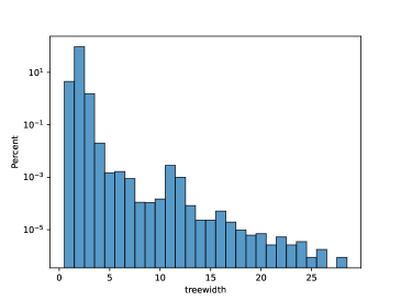
(a)

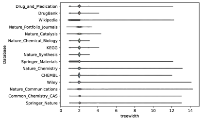
(b)

Figure 6: Distribution of treewidth for molecules in PubChem database.

4.2 Performance of our Algorithms

We now present the time vs treewidth characteristics of our algoritms for computing number of perfect matchings, matchings and independet sets (See Figure 7). The following characteristics are for selected datasets from PubChem. We have also conducted our experiments on the entire PubChem dataset. The experimental dataset will be available in the Zenedo repository.

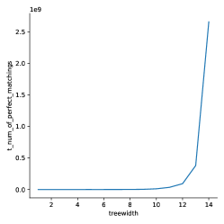
(a)

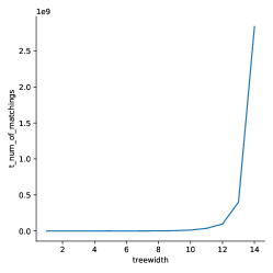
(b)

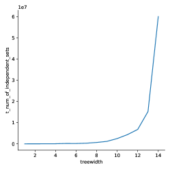
(c)

Figure 7: Time vs Treewidth characteristics for algortihms

4.3 Comparision with baseline algorithms

In this sectiom, we present a comparision of our parameterized algorithms with naive baseline algorithms (See Figure 8). We present time vs edges characteristics for graphs selected uniformly at random from selected PubChem datasources. For conducting this comparision, we limited ourselves to graphs with at most $40$ edges, and for each edge size we sampled $50$ graphs from the datasources, and reported the average time for each edge size.

(a)

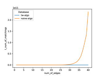
(b)

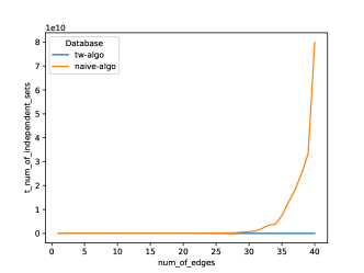
(c)

Figure 8: Comparision with baseline algorithms

4.4 Implementation Details

4.4.1 Workflow

We first downloaded SMILES [Wei88] for all PubChem compounds available using FTP bulk download option. We used open source libraries (RDKit [Che22] and pysmiles [Sof22]) to parse these SMILES to Networkx graphs [HSSC08] in Python3. Later, we used tree decomposition solver (FlowCutter) to obtain the tree decomposition for these graphs. Finally, we implemented our dynamic programming algorithms in C++ using these tree decompositions. All the statistical analysis for experiments are performed in Python3 and a detailed notebook will be provided in the resepective Zenedo repository.

4.4.2 System details

It took us nearly $3$ complete days to finish all the computations using a Linux based laptop with the following specifications: System Ubuntu 20.04.5 LTS and CPU AMD Ryzen 5 4600H with Radeon Graphics. Our entire experimental datasets and code repository will be available in Zenedo and GitHub.

5 Conclusion

In summary, we presented parameterized algorithms for $\#P$-complete problems corresponding to topological indices and graph entropies. Our algorithms, beat the known state-of-the-art methods in both computer science and chemistry literature. We also provide a first-of-its kind statistical distribution of treewidths along with a comparision of our algorithms with the baseline algorithms for the entire PubChem database of chemical compounds. We hope that the techniques and analysis in this paper would serve as an invitation to both chemists and computer scientists to use parameterized methods for computationally challenging problems in chemistry.

Authors’ addresses:

Department of Computer Science and Engineering, Hong Kong University of Science and Technology, Hong Kong
E-mail address: gkc@connect.ust.hk

Department of Computer Science and Engineering, Hong Kong University of Science and Technology, Hong Kong
E-mail address: goharshady@cse.ust.hk

Department of Mathematics: Algebra and Geometry, Ghent University, 9000 Gent, Belgium
E-mail address: harshitjitendra.motwani@ugent.be

Department of Computer Science and Engineering, Hong Kong University of Science and Technology, Hong Kong
E-mail address: snovozhilov@connect.ust.hk

References

- [CDK17] Shujuan Cao, Matthias Dehmer, and Zhe Kang. Network entropies based on independent sets and matchings. Applied Mathematics and Computation, 307:265–270, 2017.
- [CFK+15] Marek Cygan, Fedor V Fomin, Łukasz Kowalik, Daniel Lokshtanov, Dániel Marx, Marcin Pilipczuk, Michał Pilipczuk, and Saket Saurabh. Parameterized algorithms, volume 5. Springer, 2015.
- [Che22] Open Source Cheminformatics. Rdkit. https://www.rdkit.org, 2022.
- [CMR01] Bruno Courcelle, Johann A. Makowsky, and Udi Rotics. On the fixed parameter complexity of graph enumeration problems definable in monadic second-order logic. Discrete applied mathematics, 108(1-2):23–52, 2001.
- [Dea17] John C Dearden. The use of topological indices in qsar and qspr modeling. Advances in QSAR Modeling: Applications in Pharmaceutical, Chemical, Food, Agricultural and Environmental Sciences, pages 57–88, 2017.
- [Hos71] Haruo Hosoya. Topological index. a newly proposed quantity characterizing the topological nature of structural isomers of saturated hydrocarbons. Bulletin of the Chemical Society of Japan, 44(9):2332–2339, 1971.
- [HSSC08] Aric Hagberg, Pieter Swart, and Daniel S Chult. Exploring network structure, dynamics, and function using networkx. Technical report, Los Alamos National Lab.(LANL), Los Alamos, NM (United States), 2008.
- [KCC+23] Sunghwan Kim, Jie Chen, Tiejun Cheng, Asta Gindulyte, Jia He, Siqian He, Qingliang Li, Benjamin A Shoemaker, Paul A Thiessen, Bo Yu, et al. Pubchem 2023 update. Nucleic Acids Research, 51(D1):D1373–D1380, 2023.
- [MS80] Richard E Merrifield and Howard E Simmons. The structures of molecular topological spaces. Theoretica chimica acta, 55(1):55–75, 1980.
- [Sof22] Open Source Software. pysmiles. https://github.com/pckroon/pysmiles, 2022.
- [Tri18] Nenad Trinajstic. Chemical graph theory. CRC press, 2018.
- [Wei88] David Weininger. Smiles, a chemical language and information system. 1. introduction to methodology and encoding rules. Journal of chemical information and computer sciences, 28(1):31–36, 1988.
- [WTZL18] Pengfei Wan, Jianhua Tu, Shenggui Zhang, and Binlong Li. Computing the numbers of independent sets and matchings of all sizes for graphs with bounded treewidth. Applied Mathematics and Computation, 332:42–47, 2018.