Modular CSI Quantization for FDD Massive MIMO Communication

Abstract

We consider high-dimensional MIMO transmissions in frequency division duplexing (FDD) systems. For precoding, the frequency selective channel has to be measured, quantized and fed back to the base station by the users. When the number of antennas is very high this typically leads to prohibitively high quantization complexity and large feedback. In 5G New Radio (NR), a modular quantization approach has been applied for this, where first a low-dimensional subspace is identified for the whole frequency selective channel, and then subband channels are linearly mapped to this subspace and quantized. We analyze how the components in such a modular scheme contribute to the overall quantization distortion. Based on this analysis we improve the technology components in the modular approach and propose an orthonormalized wideband precoding scheme and a sequential wideband precoding approach which provide considerable gains over the conventional method. We compare the performance of the developed quantization schemes to prior art by simulations in terms of the projection distortion, overall distortion and spectral efficiency, in a scenario with a realistic spatial channel model.

I Introduction

Massive MIMO (mMIMO) communication [2] with very large antenna arrays at the base station (BS) is one of the key components in the 5G New Radio (NR). Using mMIMO in downlink, however, relies on the availability of high quality channel state information (CSI) at the transmitter (Tx). In a Frequency Division Duplex (FDD) system the channel has to be measured by the users, quantized, and then fed back to the BS. FDD MIMO finite feedback principles are well understood both in the single user [3, 4, 5] and multiuser [6, 7, 8] context. With a high number $N_{t}$ of BS antennas, however, quantization complexity and the amount of feedback can be prohibitively high. This problem becomes particularly difficult in a multiuser-MIMO setting, where the amount of feedback should scale with the Signal-to-Noise Ratio (SNR) [6]. Conventional channel feedback techniques utilize pre-defined codebooks to directly quantize and feedback the channel vector [4, 9, 10, 11]. For a desired accuracy, codebook size increases exponentially with the number of antennas, which prevents their application in massive MIMO networks, especially in frequency selective channels, where feedback is needed for each coherence bandwidth. To this end, the complexity and dimensionality for mMIMO CSI feedback needs to be reduced.

In [4] it became clear that when quantizing a complex vector in $N_{t}$ dimensions for feedback, one deals with Grassmannian quantization—the overall phase of the vector is irrelevant, and the proper concept of distance is given by the chordal distance. Vector quantization codebooks can be created, e.g., using computer search [4, 9, 10].

When the CSI to be quantized is not independent and identically distributed (i.i.d.), and the covariance matrix is known, one may perform vector quantization conditioned on the source distribution. A more practical approach, applicable to any channel covariance, was proposed in [12, 9]: an i.i.d. vector quantization codebook is constructed, and the channel covariance structure is imposed on the codebook by deforming it with the square root of the covariance.

The complexity of designing and quantizing high-dimensional CSI vectors has been addressed using product codebooks [13, 14] and trellis coded line packing [15, 16]. In these, the $N_{t}$ dimensions of the vector to be quantized are divided in parts of a lower dimension $L$, and an $L$-dimensional codebook is used to quantize the parts. These should be designed based on an Euclidean distance criterion—when combining the partial codewords, the phase becomes relevant [15], and has to be properly taken into account when combining multiple low-dimensional codewords to a higher dimensional, either when computing trellis metrics [15, 16] or by explicit quantization of combining phases [14], or by joint designs resulting in codebooks that have good distance properties both from the Euclidean and chordal distance perspective [17].

Recently, deep neural networks (DNN) have been applied for mMIMO CSI feedback [18, 19, 20]. Compared to vector quantization which imposes an overhead that grows linearly with system dimensions, and also depends on channel sparsity, DNN-based CSI feedback has promise to overcome complexity, latency and limited accuracy drawbacks in capturing CSI.

Whether basing feedback on domain knowledge or DNN, fundamental theoretical understanding on the feedback framework, quantization objectives and distortion analysis is needed as to understand the fundamental limits governing quantized CSI feedback. This motivates our work.

Of particular relevance to our work are [8, 21, 22, 23, 24, 25, 26, 27, 28] where modular/cascaded/two-tier/two-stage CSI feedback and/or covariance eigenspace quantization is considered. The low rank of mMIMO channel covariance matrices was utilized to reduce effective channel dimensionality. Modular multiuser-MIMO feedback quantization was suggested in [8, 21]. For correlated single user channels $\mathbf{h}\in\mathbb{C}^{N_{t}}$, the majority of channel energy is in a low-dimensional subspace and it is sufficient to feed back signal coordinates in this subspace. Users are clustered such that users in a cluster are assumed to share a $K$-dimensional subspace, described by an $N_{t}\times K$ unitary matrix $\mathbf{U}_{K}$. Instantaneous CSI is then fed back by the users in terms of a $K$-dimensional effective channel vector $\mathbf{c}=\mathbf{U}_{K}^{\rm H}\,\mathbf{h}$. In [22], a similar idea of two-tier precoding was pursued.

In [24, 25, 26, 27], frequency selective mMIMO channels are considered. Covariance matrices are estimated over the whole bandwidth, and narrowband effective channel CSI is created for multiple subbands. Both wideband covariance and subband CSI are quantized and fed back to the BS. In [25, 26, 27], array architecture aware precoding is performed, where the feedback is optimized for known dimensions of a planar array. In [28], two-tier precoding is performed in a multiuser MIMO setting, where one tier is a subspace for a user group, and the other for a user.

To use the modular approach in [8, 21, 22, 24, 25, 26, 27], the basis matrix ${\bf U}_{K}$ has to be quantized using a codebook ${\cal W}$. Covariance matrix and covariance eigenspace quantization has been considered in [23, 29, 21, 24, 25, 26, 30]. Matrix codebooks of unitary matrices characterizing covariance eigenspaces are considered in [23]. In [29], channel Gram matrices are constructed, and information about them is fed back using scalar quantization of matrix elements. Hierarchical quantization of $N_{t}\times K$ unitary (Stiefel) matrices as well as $K$-dimensional subspaces was considered in [31, 30, 32], where the dimensionality of the subspace decreases when proceeding in the hierarchy. In contrast, [24, 25, 26] consider independent vector quantization of the columns of $\mathbf{U}_{K}$, i.e. codebooks of the form ${\cal W}={\cal V}^{K}$, where ${\cal V}$ is a codebook of $N_{t}\times 1$ vectors. For a given quantization accuracy, the size of a vector codebook is the $K$th root of the size of a matrix codebook, which significantly reduces quantization complexity. However, when a vector codebook is used, orthogonality of the matrices cannot be guaranteed. In the matrix codebook approach of [23], orthogonality of the $K$ columns in $\mathbf{U}_{K}$ is always guaranteed. In [24], orthogonality is ensured by sequence design, limiting the vector codebook size to $N_{t}$.

To have high descriptive power with manageable complexity, high-resolution FDD feedback in 5G NR relies on overcomplete vector quantization codebooks [25, 26]. This enables high precision in describing $\mathbf{U}_{K}$, at the cost of a potential loss of orthogonality. With a non-orthogonal basis, good subband effective channel quantization might not result in good overall quantization.

In this paper, we develop a modular CSI quantization framework for massive MIMO networks with high precision and low complexity. Design objectives for both wideband quantization and subband quantization are studied, as well as codebook construction. Our major contributions are:

• We show that the overall quantization distortion decomposes into two independent parts. One describes the error of the wideband quantization of $\mathbf{U}_{K}$, the other captures effective subband channel distortion. We find a new criterion for measuring $\mathbf{U}_{K}$ quantization quality, which highlights the importance of improving wideband quantization.

• We propose orthonormalized wideband precoding (OWP) which implicitly feeds back unitary matrices despite using high precision vector codebooks for independent quantization of columns of $\mathbf{U}_{K}$. Thus despite using vector codebooks, we guarantee orthogonality of the basis in the fed back matrices, removing the drawback of using a vector codebook. Furthermore, we mitigate the loss from vector quantization by proposing a sequential wideband precoding (SWP) scheme.

• We perform simulations in an FDD mMIMO scenario, corroborating the theoretical results. Following the principles of this paper leads to considerable gains.

This paper is organized as follows. Section II introduces the system model. Section III derives the single user quantization problem from multiuser precoding. Section IV presents the modular quantization method and discusses quantization distortion partitioning. Section V introduces the wideband quantization schemes OWP and SWP. Section VI discusses subband effective channel quantization. Section VII presents simulation results, Section VIII concludes the paper.

Notation: $\mathbf{X}^{\rm T}$ and $\mathbf{X}^{\rm H}$ denote the transpose and the conjugate transpose of matrix $\mathbf{X}$, respectively. The Euclidean norm of a vector $\mathbf{x}$ is $|\mathbf{x}|$. ${\rm Tr}\,(\mathbf{X})$ denotes the trace of matrix $\mathbf{X}$.

II System Model

II-A Channel Model

We consider a Frequency Division Duplexing (FDD) multiuser multicarrier downlink massive MIMO channel in which the transmitter has $N_{t}$ antennas, and the $U$ receivers have a single antenna. The channels are frequency selective. We assume OFDM, and model frequency selectivity on a subband basis, such that there are $S$ subbands for which CSI is gathered. For simplicity we assume that the channel $\mathbf{h}_{u,s}\in\mathbb{C}^{N_{t}\times 1}$ of user $u$ on subband $s$ is the same for all subcarriers in a subband. The received signals of all the users on a subcarrier $c$ belonging to subband $s$ are

$$\mathbf{y}_{c}=\mathbf{H}_{s}\mathbf{Z}_{s}\,\mathbf{x}_{c}+\mathbf{n}_{c}\,.$$ (1)

Here $\mathbf{H}_{s}\in\mathbb{C}^{U\times N_{t}}$ is a matrix where the subband channels of the users are collected s.t. row $s$ is $\mathbf{h}_{u,s}^{\rm T}$. $\mathbf{Z}_{s}\in\mathbb{C}^{N_{t}\times U}$ is a Zero-Forcing (ZF) multiuser beamformer, $\mathbf{x}_{c}\in\mathbb{C}^{U\times 1}$ is the vector of the symbols transmitted to the users, and ${\bf n}_{c}$ is independent white Gaussian noise with variance $N_{0}$. Transmissions to different users are independent; we assume $E\{\mathbf{x}_{c}\mathbf{x}_{c}^{\rm H}\}=\mathbf{I}_{U}$. With total transmit power $P$, the power constraint then becomes ${\rm Tr}\,(\mathbf{Z}_{s}\,\mathbf{Z}_{s}^{\rm H})\leq P$.

II-B Wideband and Effective Channels

In FDD, selecting the precoder $\mathbf{Z}$ requires feeding back information from the receivers to the transmitter. We assume codebook based precoding, where each user $u$ independently quantizes its aggregate CSI $\{\mathbf{h}_{u,s}\}_{s=1}^{S}$, using a common codebook, and then feeds it back to the transmitter. As feedback is independent, when discussing channel feedback, we suppress the index $u$. We shall exploit a division to wideband and subband channels for efficient feedback.

We assume that the channel of an individual user across subbands is block Rayleigh-faded, so that it is distributed as a complex Gaussian, with a joint distribution arising from the multipath structure of the environment. The user channels on subbands are samples from this distribution, and a user has perfect knowledge of its own channels. From these, a user can construct a sample covariance matrix which is an estimate of $E_{\mathbf{h}}\left\{\,\mathbf{h}\,\mathbf{h}^{\rm H}\right\}$. This form of the covariance is used in the literature for capturing the wideband characteristic of the channel [24, 23, 26]. However, in this paper we shall prove that the normalized sample covariance

$$\widetilde{\mathbf{R}}=\sum_{s}\mathbf{h}_{s}\,\mathbf{h}_{s}^{{\rm H}}/\left|\mathbf{h}_{s}\right|^{2}=\sum_{s}\tilde{\mathbf{h}}_{s}\,\tilde{\mathbf{h}}_{s}^{{\rm H}}$$ (2)

should be applied for feedback optimization. Here we defined the normalized subband channel $\tilde{\mathbf{h}}_{s}=\mathbf{h}_{s}/\left|\mathbf{h}_{s}\right|$. Note that the sample covariance is user specific.

The aggregate CSI is captured by the sample covariance $\widetilde{\mathbf{R}}$ describing the wideband characteristics of the channel, and subband specific coordinates describing the subband channels in the basis given by $\widetilde{\mathbf{R}}$. Note that the normalization in (2) does not change the fact that eigenvectors of $\widetilde{\mathbf{R}}$ span a subspace in which all $h_{s}$ lie. We have the eigenvalue decomposition

$$\widetilde{\mathbf{R}}=\mathbf{U}\mathbf{\Lambda}\mathbf{U}^{\rm H},$$ (3)

where for ${\rm rank}(\widetilde{\mathbf{R}})=r\leq N_{t}$, $\mathbf{\Lambda}$ is an $r\times r$ diagonal matrix of $r$ positive eigenvalues arranged in descending order, and $\mathbf{U}=[\mathbf{u}_{1},\mathbf{u}_{2},\dots,\mathbf{u}_{r}]$ is the tall unitary $N_{t}\times r$ matrix consisting of the corresponding eigenvectors $\mathbf{u}_{j}$. We also define the singular values $\sigma_{j}=\sqrt{\lambda_{j}},\,j=1,\ldots,r$, and the matrix $\mathbf{\Sigma}=\operatorname{diag}(\{\sigma_{j}\})=\sqrt{\mathbf{\Lambda}}$ of singular values of $\sqrt{\widetilde{\mathbf{R}}}$. We have $\mathbf{U}^{\rm H}\mathbf{U}=\mathbf{I}_{r}$, the $r$-dimensional identity matrix, while $\mathbf{U}\mathbf{U}^{\rm H}=\mathbf{\Pi}_{r}$ is a projector to the $r$-dimensional eigenspace of $\widetilde{\mathbf{R}}$. By construction we have $\mathbf{\Pi}_{r}\mathbf{h}_{s}=\mathbf{h}_{s}$.

Given $\widetilde{\mathbf{R}}$, the subband channel vectors can be expressed in two ways as ideal subband effective channels: $\mathbf{h}_{s}=\mathbf{U}\,\mathbf{b}_{s}=\mathbf{U}\,\mathbf{\Sigma}\,\mathbf{c}_{s}$, where $\mathbf{b}_{s}$ and $\mathbf{c}_{s}$ are $r\times 1$ vectors, given by

$$\mathbf{b}_{s} = \mathbf{U}^{\rm H}\mathbf{h}_{s}$$ (4)

$$\mathbf{c}_{s} = {\mathbf{\Sigma}}^{-1}\mathbf{b}_{s}={\mathbf{\Sigma}}^{-1}\mathbf{U}^{\rm H}\mathbf{h}_{s}\,.$$ (5)

We have $|\mathbf{b}_{s}|=|\mathbf{h}_{s}|$, while the transformation to $\mathbf{c}_{s}$ does not preserve norm, $\mathbf{c}_{s}^{\rm H}\mathbf{\Lambda}\mathbf{c}_{s}=|\mathbf{h}_{s}|^{2}$.

The sample covariances of $\mathbf{b}$ and $\mathbf{c}$ with the same normalization as in $\widetilde{\mathbf{R}}$ are

$$\sum_{s=1}^{S}\mathbf{b}_{s}\mathbf{b}_{s}^{\rm H}=\mathbf{\Lambda}\,,~{}~{}~{}~{}\sum_{s=1}^{S}\mathbf{c}_{s}\mathbf{c}_{s}^{\rm H}=\mathbf{I}\,.$$ (6)

The coordinates in $\mathbf{b}_{s}$ are thus independently but non-identically distributed (i.n.i.d.) while the effective channel coordinates $\mathbf{c}_{s}$ are i.i.d.

III Zero Forcing Precoding with Incomplete CSI at Tx

The transmitter constructs a multiuser ZF precoder per subband $s$, used on each subcarrier channel (1) belonging to the subband, based on incomplete CSI fed back by the users to the Tx. We divide the CSI to Channel Direction Information (CDI), quantizations $\hat{\mathbf{h}}_{u,s}$ of the normalized channel vectors $\tilde{\mathbf{h}}_{u,s}$, and Channel Amplitude Information (CAI) $\hat{q}_{u,s0}>0$, quantizing $|\mathbf{h}_{u,s}|$. The CDI takes values in a user-specific quantization codebook, $\hat{\mathbf{h}}_{u,s}\in{\mathcal{H}}$.

III-A Bound on Expected Rate

The CDI of the users on the subband are collected to the $U\times N_{t}$ matrix $\hat{\mathbf{H}}_{s}$, where row $u$ is $\mathbf{h}_{u,s}^{\rm T}$. We also divide the precoder to a normalized part $\widetilde{\mathbf{Z}}$ and a diagonal power allocation part $\mathbf{A}_{s}$ with diagonal elements $a_{u,s}$, as

$$\mathbf{Z}_{s}=\widetilde{\mathbf{Z}}_{s}\mathbf{A}_{s}\,,$$ (7)

were $\left|\mathbf{z}_{u,s}\right|=1$. The power constraint now reads ${\rm Tr}\left({\widetilde{\mathbf{Z}}_{s}}^{\rm H}\widetilde{\mathbf{Z}}_{s}\,\mathbf{A}_{s}^{2}\right)\leq P$. As the subspace spanned by a set vectors equals the subspace spanned by the corresponding normalized versions, $\widetilde{\mathbf{Z}}$ does not depend on CAI, we have $\widetilde{\mathbf{Z}}_{s}=\widetilde{\mathbf{Z}}_{s}\left(\hat{\mathbf{H}}_{s}\right)$. The ZF precoding vector $\tilde{\mathbf{z}}_{u}$ is defined as a unit norm vector in the subspace spanned by $\hat{\mathbf{H}}_{s}^{*}$, s.t. $\mathbf{h}_{v,s}^{\rm T}\mathbf{z}_{u}=0$ for all $v\neq u$.

Assuming that $\mathbf{x}_{c}$ in (1) are independent, and independent from the noise, the Signal-to-Interference-plus-Noise Ratio (SINR) on subband $s$ at user $u$ becomes:

$$\gamma_{u,s} = \frac{\left|\mathbf{h}_{u,s}^{\rm T}\mathbf{z}_{u}\right|^{2}}{\sum_{v\neq u}\left|\mathbf{h}_{u,s}^{\rm T}\mathbf{z}_{v}\right|^{2}+N_{0}}$$ (8)

$$= \frac{\rho_{u,s}\,\left|\tilde{\mathbf{h}}_{u,s}^{\rm T}\tilde{\mathbf{z}}_{u}\right|^{2}}{1+\rho_{u,s}\sum_{v\neq u}\frac{a_{v}^{2}}{a_{u}^{2}}\left|\tilde{\mathbf{h}}_{u,s}^{\rm T}\tilde{\mathbf{z}}_{v}\right|^{2}}~{},$$ (9)

where $\rho_{u,s}=a_{u}^{2}\,\left|\mathbf{h}_{s,u}\right|/N_{0}$ is the Signal-to-Noise Ratio (SNR) of user $u$ on subband $s$. Assuming Gaussian codebooks the rate of user $u$ on subband $s$ is lower bounded as [6]

$$R_{u,s} = \ln\left(1+\gamma_{u,s}\right)\geq\ln\left(1+\rho_{u,s}\,\left|\tilde{\mathbf{h}}_{u,s}^{\rm T}\tilde{\mathbf{z}}_{u}\right|^{2}\right)$$ (11)

$$-\ln\left(1+\rho_{u,s}\sum_{v\neq u}\frac{a_{v}^{2}}{a_{u}^{2}}\left|\tilde{\mathbf{h}}_{u,s}^{\rm T}\tilde{\mathbf{z}}_{v}\right|^{2}\right)\,.$$

We assume that a user grouping principle is applied to select the $U$ users served in the subband, e.g., users with near-orthogonal channels $\hat{\mathbf{h}}_{u,s}$ may be selected. This results in a distribution of $\beta_{u}=\left|\hat{\mathbf{h}}_{u,s}^{\rm T}\tilde{\mathbf{z}}_{u}\right|^{2}\in[0,1]$. We furthermore assume a power allocation principle that jointly selects the amplitudes $a_{u,s}$ for all the users, based on the CAI $q_{u,s}$ and the realizations of $\beta_{u}$.

The true channel direction can expressed in terms of the quantized CDI as

$$\tilde{\mathbf{h}}_{u,s}=\sqrt{1-\epsilon^{2}}\,\hat{\mathbf{h}}_{u,s}+\epsilon_{\|}\,\mathbf{e}_{\|}+\epsilon_{\perp}\,\mathbf{e}_{\perp}\,,$$ (12)

where quantization error has two parts, one in the subspace spanned by the other user’s channels $\left\{\mathbf{h}_{v,s}\right\}_{v\neq u}$, another in the subspace orthogonal to all user’s channels. The directions of these are given by the unit vectors $\mathbf{e}_{\|}$, and $\mathbf{e}_{\perp}$, respectively, and the magnitudes add up as $\epsilon_{\|}^{2}+\epsilon_{\perp}^{2}=\epsilon^{2}$. In the wanted signal component in (11) we thus have

$$\left|\tilde{\mathbf{h}}_{u,s}^{\rm T}\tilde{\mathbf{z}}_{u}\right|^{2}=(1-\epsilon^{2})\left|\hat{\mathbf{h}}_{u,s}^{\rm T}\tilde{\mathbf{z}}_{u}\right|^{2}=(1-\epsilon^{2})\beta_{u}\,,$$

and in the interference-part

$$\left|\tilde{\mathbf{h}}_{u,s}^{\rm T}\tilde{\mathbf{z}}_{v}\right|^{2}=\epsilon_{1}^{2}\left|{\mathbf{e}_{\|}}^{\rm T}\tilde{\mathbf{z}}_{v}\right|^{2}=\epsilon_{1}^{2}\delta_{u,v}\leq\epsilon^{2}\delta_{u,v}\,,$$

for some $\delta_{u,v}\in[0,1]$.

In [6], the distribution of quantization error was derived for the case $U=N_{t}$, with channels chosen uniformly at random, equal power allocation and random vector quantization, leading to a lower bound on the rate. This can be extended to any $U$, user grouping, power allocation and quantization codebook as follows.

For a user of interest, we average over the possible channel states $\mathbf{h}_{s}$, and all possible other user’s channels given by a grouping principle. We assume that the quantization of $\tilde{\mathbf{h}}_{u,s}$ in ${\mathcal{H}}$ is homogeneous; the magnitude $\epsilon$ of the quantization error is independent of $\hat{\mathbf{h}}_{u,s}$ and the directions $\mathbf{e}_{\|}$, $\mathbf{e}_{\perp}$. From the variables effecting the SINR, the power allocation amplitudes $a_{v}$, the SNR $\rho$ and the inner product $\beta$ are thus jointly distributed, while $\epsilon$ and the $\delta_{u,v}$ are independent.

With the definitions above, the rate bound (11) becomes

$$R_{u,s}\geq\ln\left(1+(1-\epsilon^{2})\rho\,\beta\right)-\ln\left(1+\epsilon^{2}\rho\sum_{v\neq u}\frac{a_{v}^{2}}{a_{u}^{2}}\delta_{u,v}\right)\,.$$

where we dropped the subscript from $\rho$ and $\beta$. The first term $R_{1}$ can be further bounded as

$$R_{1} \geq \ln\left(1+\rho\,\beta\right)+\ln\left(1-\epsilon^{2}\right)$$

$$\geq \ln\left(1+\rho\,\beta\right)-\frac{\epsilon^{2}}{1-\epsilon^{2}}\,\geq\,\ln\left(1+\rho\,\beta\right)-\epsilon^{2}\,.$$

We used the inequality $x/(1+x)\leq\ln(1+x)$, valid for $x\geq-1$ [33]. When averaging over the channels, the second term can be bounded using Jensen’s inequality. Defining $C_{1}=E_{\beta,\rho}\left\{\ln(1+\rho\,\beta)\right\}$ and $C_{2}=E_{\rho,a,\mathbf{\delta}}\left\{\rho\sum_{v\neq u}\frac{a_{v}^{2}}{a_{u}^{2}}\delta_{u,v}\right\}$, we get a lower bound for the expected rate:

$$E_{\beta,\rho,a,\mathbf{\delta},\epsilon}\left\{R\right\}\geq C_{1}-E_{\epsilon}\left\{\epsilon^{2}\right\}-\ln\left(1+C_{2}\,E_{\epsilon}\left\{\epsilon^{2}\right\}\right)\,.$$ (13)

III-B Quantization Distortion

The chordal distance between two vectors $\mathbf{x}$ and $\mathbf{y}$ is

$$d(\mathbf{x},\mathbf{y})=\sqrt{1-\frac{|\mathbf{x}^{\rm H}\mathbf{y}|^{2}}{|\mathbf{x}|^{2}|\mathbf{y}|^{2}}}\,.$$ (14)

According to (12), the quantization error is given by the chordal distance, $\epsilon^{2}=d^{2}(\tilde{\mathbf{h}}_{s},\hat{\mathbf{h}})=d^{2}(\mathbf{h}_{s},\hat{\mathbf{h}})$. From (13) it follows that the lower bound on rate is maximized if the codebook ${\mathcal{H}}$ for quantizing $\mathbf{h}_{s}$ is chosen to minimize the quantization distortion

$$D_{\mathcal{H}}=E_{\mathbf{h}_{s}}\left\{\underset{\hat{\mathbf{h}}\in{\mathcal{H}}}{\mathrm{min}}\,d^{2}(\mathbf{h}_{s},\hat{\mathbf{h}})\right\}=\sum_{\hat{\mathbf{h}}\in{\mathcal{H}}}E_{V(\hat{\mathbf{h}})}\left\{d^{2}(\mathbf{h}_{s},\hat{\mathbf{h}})\right\}\,.$$ (15)

In the second expression, the distortion has been written as a sum over the division of the domain of $\mathbf{h}_{s}$ to Voronoi cells $V(\hat{\mathbf{h}})=\{\mathbf{h}\mid\arg\min_{\mathbf{q}\in{\mathcal{H}}}\,d(\mathbf{h},\mathbf{q})=\hat{\mathbf{h}}\}$ centered at the codewords $\hat{\mathbf{h}}\in{\mathcal{H}}$.

Our goal is to develop quantization schemes that minimize distortion. Note that the distortion expressly considers quantization of channel direction only. For the bound (13), the quantization error in $|\mathbf{h}_{s}|$ irrelevant. The decoupling of CDI and CAI quantization is a consequence of ZF.

IV Modular Single User CSI Quantization

In this section, the overall process of the developed modular CSI quantization approach for a single-user codebook ${\mathcal{H}}$ will be presented, followed by a discussion on partitioning quantization distortion between wideband and subband quantization.

IV-A Basic idea and earlier works of modular quantization

If the subband channels $\mathbf{h}_{s}$ come from an arbitrary distribution, their quantization and feedback can be highly complex. However, if we can assume that the channels from different antennas are correlated, it is possible to apply modular quantization [8, 21, 22, 24, 27] and reduce complexity considerably. In this section we shortly review some of the known results and then present our approach.

IV-A1 Modular quantization with ideal wideband quantization

Let us assume that the covariance matrix $\mathbf{R}$ is fixed and we have a budget of bits for feeding back wideband statistical data of the channel pertaining to $\mathbf{R}$, and a separate budget for feeding back subband specific CSI pertaining to the coordinates $\mathbf{c_{s}}$. In the extreme case with unlimited wideband feedback, the BS knows $\mathbf{U}$ and $\mathbf{\Lambda}^{1/2}$ perfectly. For limited feedback, we make the rank-$K$ approximation of the covariance matrix. We denote with $\mathbf{U}_{K}$ the $N_{t}\times K$ matrix consisting of columns of $\mathbf{U}$ ordered by the size of the corresponding eigenvalues, and $\mathbf{\Lambda}$ and $\mathbf{\Sigma}$ are now $K\times K$ diagonal matrices with the $K$ largest eigen- and singular values.

Ideal subband quantization would then proceed as follows. Given $\mathbf{U}_{K}$, the subband effective channel vectors can be expressed in two ways as

$$\mathbf{b}_{s} = \mathbf{U}_{K}^{\rm H}\mathbf{h}_{s}$$ (16)

$$\mathbf{c}_{s} = {\mathbf{\Sigma}}^{-1}\mathbf{b}_{s}={\mathbf{\Sigma}}^{-1}\mathbf{U}_{K}^{\rm H}\mathbf{h}_{s}\,,$$ (17)

where $\mathbf{b}_{s}$ and $\mathbf{c}_{s}$ are length $K$ random vectors. Note that $\mathbf{c}_{s}$ is typically not unit norm. However, as the bound (13) is in terms of chordal distance and does not depend on $|\mathbf{h}_{s}|$, we may normalize $\mathbf{c}_{s}$. The user then quantizes $\mathbf{c}_{s}$ to $\hat{\mathbf{c}}_{s}$ using a $K$-dimensional Grassmannian line codebook $\hat{\mathcal{C}}\subset{\cal G}_{\mathbb{C}}(K,1)$ and feeds this information to the BS. The BS can construct an estimate of $\mathbf{h}_{s}$ as

$$\hat{\mathbf{h}}_{s}=\mathbf{U}_{K}\mathbf{\Sigma}\hat{\mathbf{c}}_{s}.$$ (18)

The key point is that the modular approach reduces the dimension of subband quantization from $N_{t}$ to $K$. Due to the unitarity of $\mathbf{U}_{K}$, good quantization on the effective channel should lead in good quantization on the actual channel, as $\mathbf{U}_{K}$ captures most of the energy of $\mathbf{h}_{s}$.

IV-A2 Wideband quantization

For wideband feedback, either a codebook of orthogonal matrices [23, 28] or a vector codebook $\hat{\mathcal{C}}_{\mathbf{w}}$ for quantizing the $N_{t}\times 1$ columns in $\mathbf{U}_{K}$ [27, 26] can be used. A scalar codebook is used for quantizing the elements in $\mathbf{\Sigma}$ [26]. After wideband CSI feedback, the BS has a matrix $\mathbf{V}$, which is a quantized version of $\mathbf{U}_{K}$, and $\hat{\mathbf{\Sigma}}$, which is a quantized version of $\mathbf{\Sigma}$. Subband quantization now proceeds as in (17,18) but replacing $\mathbf{U}_{K}$ with $\mathbf{V}$ and $\mathbf{\Sigma}$ with $\hat{\mathbf{\Sigma}}$. However, if the vector codebook $\hat{\mathcal{C}}_{\mathbf{w}}$ is overcomplete, as for example in the high resolution alternative of 5G NR [25], there is a high probability that $\mathbf{V}$ is not unitary, and the connection between the channel and effective channel quantization is partially broken. In the following we will show how we can avoid this problem.

IV-B Outline of the Suggested CSI Quantization Method

In this section we will shortly describe our approach to the quantization problem. In later sections we will elaborate on each part of the quantization process.

While conventionally wideband feedback is based on quantizing the covariance matrix $\mathbf{R}=E_{\mathbf{h}}\left\{\mathbf{h}\mathbf{h}^{{\rm H}}\right\}$ [24], or a normalized version $E_{\mathbf{h}}\left\{\mathbf{h}\mathbf{h}^{{\rm H}}\right\}/E_{\mathbf{h}}\left\{|\mathbf{h}|^{2}\right\}$ [26], we instead quantize $\widetilde{\mathbf{R}}$ of (2) and its singular value decomposition. The motivation for this will be given in Section IV-C.

Aiming at $K$-dimensional effective channel feedback, we proceed by quantizing $\mathbf{U}_{K}$ column by column using some vector quantization codebook $\hat{\mathcal{C}}_{\mathbf{w}}$. As a result the user has now an $N_{t}\times K$ matrix $\mathbf{V}$ consisting of quantized norm $1$ vectors, which are fed back to the BS. These vectors are not necessarily orthonormal.

However, we assume that the users and the base-station have agreed on a method to orthonormalize the vectors $\mathbf{V}$ to a set of column vectors $\mathbf{W}$ with $\mathbf{W}^{\rm H}\mathbf{W}=\mathbf{I}_{K}$ and ${\rm span}(\mathbf{W})={\rm span}(\mathbf{V})$. This method is independent of the structure of $\mathbf{V}$ and is assumed to be shared at the same time as the codebook $\hat{\mathcal{C}}_{\mathbf{w}}$. Both the user and the BS perform this operation, after which they both have the same matrix $\mathbf{W}$. Exactly the same number of bits can be used to feed back this matrix as feeding back the original $\mathbf{V}$. The matrix $\mathbf{W}$ is now used in place of $\mathbf{V}$ for the rest of the quantization.

As $\mathbf{V}$ is transformed to $\mathbf{W}$ the singular values computed from (3) do not characterize the relative weight of the columns in $\mathbf{W}$ when describing subbands. Instead, for each column $\mathbf{w}_{j}$ in $\mathbf{W}$, the user calculates wideband amplitudes

$$\sigma_{j}=\sqrt{\mathbf{w}_{j}^{\rm H}\widetilde{\mathbf{R}}\mathbf{w}_{j}}$$ (19)

and feeds back their scalar quantized versions $\hat{\sigma}_{j}$ constituting the diagonal matrix $\hat{\mathbf{\Sigma}}$.

After this, BS and user share the matrix $\mathbf{W}$ and the quantized wideband amplitude matrix $\hat{\mathbf{\Sigma}}$. Using these matrices, the subband feedback can be performed as in Equations (17) and (18), replacing $\mathbf{U}_{K}$ and $\mathbf{\Sigma}$ with $\mathbf{W}$ and $\hat{\mathbf{\Sigma}}$. The reconstruction of the channel can be done as

$$\hat{\mathbf{h}}_{s}=\mathbf{W}\hat{\mathbf{\Sigma}}\hat{\mathbf{c}}_{s}.$$

When $\mathbf{W}$ and $\hat{\mathbf{\Sigma}}$ are fixed, then any quantization codebook $\mathcal{C}\subset\mathbb{C}^{K}$, designed to quantize a $K$-dimensional effective channel $\mathbf{c}_{s}=\hat{\mathbf{\Sigma}}^{-1}\mathbf{W}^{{\rm H}}\mathbf{h_{s}}$, induces a codebook [12, 9]

$${\cal B}=\left\{\frac{\hat{\mathbf{\Sigma}}\hat{\mathbf{c}}}{|\hat{\mathbf{\Sigma}}\hat{\mathbf{c}}|}\,\,\Big{|}\,\,\hat{\mathbf{c}}\in{\cal C}\right\}\,,$$ (20)

which quantizes the $K$-dimensional effective channel $\mathbf{W}^{H}\mathbf{h}_{s}=\mathbf{b}_{s}.$ Furthermore it also induces a codebook for the actual $N_{t}\times 1$ channel $\mathbf{h}_{s}$ by

$${\mathcal{H}}=\mathbf{W}\,{{\cal B}}=\{\hat{\mathbf{h}}=\mathbf{W}\,\hat{\mathbf{b}}\,\mid\,\hat{\mathbf{b}}\in{{\cal B}}\}\,.$$ (21)

The whole quantization process can now be divided to three steps: spatial compression and wideband quantization, dimensionally reduced subband quantization, and reconstruction. The users and the BS share information about the quantization process, and the codebooks $\cal H,B,C$. A flowchart is presented in Fig. 1. The flowchart also contains terms that are not yet defined, but we will elaborate on them later on.

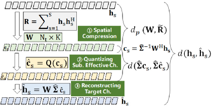
Figure 1: Flowchart for general process of CSI quantization.

IV-C Quantization Distortion Partitioning

To design a modular quantization scheme, we should understand how the wideband and subband components in the quantization procedure affect the overall quantization distortion. We start by analyzing the overall subband channel distortion when using a generic $N_{t}\times K$ wideband precoder $\mathbf{V}$, resulting from a wideband quantization procedure.

As orthogonality of vectors may be lost in quantization, a generic quantized $N_{t}\times K$ wideband beamforming matrix $\mathbf{V}$ may not be orthogonal. We can orthogonalize it as:

$$\mathbf{V}=\mathbf{W}\mathbf{C}^{-1}$$ (22)

where $\mathbf{W}$ is an $N_{t}\times K$ Stiefel matrix satisfying $\mathbf{W}^{\rm H}\mathbf{W}=\mathbf{I}$ and $\mathbf{C}$ is a $K\times K$ matrix fulfilling $\mathbf{C}\mathbf{C}^{\rm H}=\left(\mathbf{V}^{\rm H}\mathbf{V}\right)^{-1}$. If Gram-Schmidt orthogonalization is used, (22) is the QR-decomposition of $\mathbf{V}$, with $\mathbf{C}$ the upper triangular Cholesky factor of the basis correlation matrix. The wideband beamformer defines a projection operator

$$\mathbf{\Pi}_{W}=\mathbf{V}\left(\mathbf{V}^{\rm H}\mathbf{V}\right)^{-1}\mathbf{V}^{\rm H}=\mathbf{W}\mathbf{W}^{\rm H}$$ (23)

mapping $\mathbb{C}^{N_{t}}$ to the $K$-dimensional subspace spanned by the columns of $\mathbf{V}$ (and $\mathbf{W}$).

We have a codebook ${\mathcal{H}}$ to quantize $N_{t}$-dimensional subband channels $\mathbf{h}:=\mathbf{h}_{s}$. According to (14)-(15) we are interested in how well the elements of ${\mathcal{H}}$ quantize $\mathbf{h}$ in terms of chordal distance. Hence, all the codewords $\hat{\mathbf{h}}\in{{\mathcal{H}}}$ satisfy $|\hat{\mathbf{h}}|=1$.

We can now decompose $\mathbf{h}$ to a component $\mathbf{h}_{\|}$ lying in the column space of $\mathbf{W}$, and to a component $\mathbf{h}_{\perp}$ in the perpendicular subspace, lost in wideband quantization;

$$\mathbf{h}=\mathbf{\Pi}_{W}\mathbf{h}+(\mathbf{I}-\mathbf{\Pi}_{W})\mathbf{h}:=\mathbf{h}_{\|}+\mathbf{h}_{\perp}~{}.$$ (24)

We use shorthand notations $\tilde{\mathbf{h}}=\mathbf{h}/|\mathbf{h}|$, $\tilde{\mathbf{h}}_{\|}=\mathbf{\Pi}_{\mathbf{W}}\tilde{\mathbf{h}}=\mathbf{h}_{\|}/|\mathbf{h}|$ and $\tilde{\mathbf{h}}_{\perp}=\mathbf{h}_{\perp}/|\mathbf{h}|$. These fulfill

$$|\tilde{\mathbf{h}}|^{2}=|\tilde{\mathbf{h}}_{\|}|^{2}+|\tilde{\mathbf{h}}_{\perp}|^{2}=1.$$ (25)

As $\hat{\mathbf{h}}$ is in the span of $\mathbf{W}$ we have $\tilde{\mathbf{h}}^{\rm H}\hat{\mathbf{h}}=\tilde{\mathbf{h}}_{\|}^{\rm H}\hat{\mathbf{h}}$. The distortion can thus be decomposed as

$$d^{2}(\mathbf{h},\hat{\mathbf{h}})=|\tilde{\mathbf{h}}_{\|}|^{2}~{}d^{2}(\mathbf{h}_{\|},\hat{\mathbf{h}})+|\tilde{\mathbf{h}}_{\perp}|^{2}\,.$$ (26)

There is a component related to the distortion in the subspace spanned by $\mathbf{V}$, and a component arising from the part lost in wideband quantization.

For a $\mathbf{W}$ and a normalized covariance $\mathbf{R}$ with ${\rm Tr}\,(\mathbf{R})=1$, we define the projection distortion

$$d_{p}(\mathbf{W},\mathbf{R})=1-{\rm Tr}\left(\mathbf{\Pi}_{\mathbf{W}}\,\mathbf{R}\right)\,.$$ (27)

With $\mathbf{U}$ and $\mathbf{\Sigma}$ the eigenvector and singular value matrices of $\mathbf{R}$, we see that this is nothing but the squared Euclidean distance between $\mathbf{U}\mathbf{\Sigma}$ and its projection to $\mathbf{W}$:

$$d_{p}\left(\mathbf{W},\mathbf{U}\mathbf{\Sigma}^{2}\mathbf{U}^{\rm H}\right)=\left\|\mathbf{U}\mathbf{\Sigma}-\mathbf{\Pi}_{\mathbf{W}}\mathbf{U}\mathbf{\Sigma}\right\|_{F}^{2}\,.$$ (28)

For $\mathbf{W}$ of (22) an orthogonalization of $\mathbf{V}$, we have $d_{p}(\mathbf{W},\mathbf{R})=d_{p}(\mathbf{V},\mathbf{R})$.

As the projection operator $\mathbf{\Pi}_{W}$ maps $\mathbb{C}^{N_{t}}$ to the $K$-dimensional subspace spanned by the columns of $\mathbf{W}$, the projection distortion measures the amount of power of $\mathbf{R}$ outside the column space of the wideband beamformer $\mathbf{W}$. To minimize distortion, the wideband beamformer $\mathbf{V}$ should capture as much power as possible from the covariance matrix $\mathbf{R}$ in its column space. As such, the projection distortion measures the accuracy of wideband quantization.

We can now formulate the central result of this paper, governing the partition of quantization distortion between wideband and subband quantization:

Proposition 1

Given an ensemble of random $N_{t}\times 1$ vectors $\mathbf{h}$, an $N_{t}\times K$ matrix $\mathbf{W}$ and a quantization codebook ${{\mathcal{H}}}$ in the subspace spanned by $\mathbf{W}$, the quantization distortion is

$$D_{\mathcal{H}}=E_{\mathbf{h}}\left\{|\tilde{\mathbf{h}}_{\|}|^{2}\,\underset{\hat{\mathbf{h}}\in{\mathcal{H}}}{\min}~{}d^{2}\!\!\left(\mathbf{h}_{\|},\hat{\mathbf{h}}\right)\right\}+d_{p}(\mathbf{W},\widetilde{\mathbf{R}})$$

where $\widetilde{\mathbf{R}}$ is the covariance (2) of normalized vectors $\tilde{\mathbf{h}}$, $d_{p}$ is the projection distortion of (27), and $\mathbf{h}_{\|}=\mathbf{\Pi}_{W}\mathbf{h}$, with $\mathbf{\Pi}_{W}$ the projector to the column space of $\mathbf{W}$.

Proof:

Following (15), we first compute the expectation over $\mathbf{h}$ in a Voronoi cell $V$ with centroid $\hat{\mathbf{h}}$. From (26) we get

$$E_{V}\left\{d^{2}(\mathbf{h},\hat{\mathbf{h}})\right\}=E_{V}\left\{|\tilde{\mathbf{h}}_{\|}|^{2}d^{2}(\mathbf{h}_{\|},\hat{\mathbf{h}})\right\}+E_{V}\left\{|\tilde{\mathbf{h}}_{\perp}|^{2}\right\}.$$

It follows from (25) that

$$E_{V}\left[|\tilde{\mathbf{h}}_{\perp}|^{2}\right] =1-E_{V}\left[|\tilde{\mathbf{h}}_{\|}|^{2}\right]=1-E_{V}\left[{\rm Tr}(\mathbf{\Pi}_{W}\tilde{\mathbf{h}}\tilde{\mathbf{h}}^{\rm H})\right]\,.$$

Since the expected value commutes with trace and multiplication with constant matrices, the expectation acts only on $\tilde{\mathbf{h}}\tilde{\mathbf{h}}^{\rm H}$ in the last term. The result follows by summing over all Voronoi cells, and using (2). ∎

Here $\widetilde{\mathbf{R}}$ is indeed the covariance of the directions $\tilde{\mathbf{h}}$ of the subband channel vectors, the channels are normalized before computing the covariance. It is normalized as:

$${\rm Tr}\,(\widetilde{\mathbf{R}})=E_{\mathbf{h}}\left\{{\rm Tr}\,(\tilde{\mathbf{h}}\tilde{\mathbf{h}}^{\rm H})\right\}=E_{\mathbf{h}}\left\{\tilde{\mathbf{h}}^{\rm H}\tilde{\mathbf{h}}\right\}=1\,,$$ (29)

thus the projection distortion is well-defined for it.

It is worth noting that minimum distortion quantization in Proposition 1 is performed in the codebook ${\mathcal{H}}$ of $N_{t}$-dimensional vectors. To reduce subband quantization complexity, quantization should be performed directly on $K$-dimensional effective channels $\mathbf{b}$ or $\mathbf{c}$. We thus use a codebook ${\cal B}$ to quantize the $K\times 1$ effective channels. With wideband precoder $\mathbf{V}$, the induced codebook for $\mathbf{h}$ is ${\mathcal{H}}=\mathbf{V}\,{{\cal B}}=\{\hat{\mathbf{h}}=\mathbf{V}\,\hat{\mathbf{b}}\,\mid\,\hat{\mathbf{b}}\in{{\cal B}}\}\,.$ $K$-dimensional minimum chordal distance quantization

$$\hat{\mathbf{b}}=\arg\min_{\hat{\mathbf{b}}\in{\cal B}}\{\,d(\mathbf{b},\hat{\mathbf{b}})\,\}$$ (30)

may now be performed, given effective channels $\mathbf{b}$. For the resulting $N_{t}$-dimensional codeword $\mathbf{V}\hat{\mathbf{b}}$ to be the same as the minimum distance codeword $\arg\min_{\hat{\mathbf{h}}\in\mathbf{V}{\cal B}}d(\mathbf{h},\hat{\mathbf{h}})$ in $N_{t}$ dimensions, the mapping $\mathbf{V}$ between $N_{t}$ and $K$ dimensions has to preserve chordal distance. We have:

Lemma 1

Consider a linear mapping $\mathbf{V}\in\mathbb{C}^{N_{t}\times K}$ mapping $\mathbf{b}\in\mathbb{C}^{K}$ to $\mathbf{h}=\mathbf{V}\mathbf{b}\in\mathbb{C}^{N_{t}}$. $\mathbf{V}$ is an isometry w.r.t. the chordal distance,

$$d(\mathbf{h}_{1},\mathbf{h}_{2})=d(\mathbf{b}_{1},\mathbf{b}_{2}),$$ (31)

if and only if $\mathbf{V}^{\rm H}\mathbf{V}\sim\mathbf{I}_{K}$.

Proof:

Let us assume that $\mathbf{V}^{\rm H}\mathbf{V}\sim\mathbf{I}_{K}$. Recalling (14) and noticing that

$$|(\mathbf{V}\mathbf{h}_{1})^{{\rm H}}\mathbf{V}\mathbf{h}_{2}|=|\mathbf{h}_{1}^{{\rm H}}\mathbf{h}_{2}|$$

it follows that orthogonality implies isometry. To complete the proof, we need to show that non-orthogonality implies non-isometry. For this, first assume that $\mathbf{V}^{\rm H}\mathbf{V}=\mathbf{C}$, with an off-diagonal element $c_{ij}\neq 0$ for some $i\neq j$. Take the $K$-dimensional unit vectors $\mathbf{e}_{i}$ and $\mathbf{e}_{j}$. These are orthogonal, such that $d(\mathbf{e}_{i},\mathbf{e}_{j})=1$. In the $N_{t}$-dimensional space, $\mathbf{V}\mathbf{e}_{i}$ and $\mathbf{V}\mathbf{e}_{j}$ have a non-vanishing inner product. This is not changed by normalization, thus $d(\mathbf{V}\mathbf{e}_{i},\mathbf{V}\mathbf{e}_{j})<1$. If $\mathbf{C}$ is diagonal, but not proportional to identity, there exists some $i,j$ for which $c_{ii}\neq c_{jj}$. Now the chordal distance between the $K$-dimensional vectors $\mathbf{e}_{i}$ and $\left(\mathbf{e}_{i}+\mathbf{e}_{j}\right)/\sqrt{2}$ is not preserved by $\mathbf{V}$. ∎

For an orthogonal wideband precoder $\mathbf{W}$, we define the subband quantization distortion of (30) as

$$D_{\cal B}=E_{\mathbf{h}}\left\{\min_{\hat{\mathbf{b}}\in{\cal B}}d^{2}(\mathbf{W}^{\rm H}\mathbf{h},\hat{\mathbf{b}})\right\}\,.$$ (32)

From the results above it now follows

Corollary 1

For quantization codebook ${\mathcal{H}}=\mathbf{W}{\cal B}$ with orthogonal $\mathbf{W}$, the overall distortion is upper and lower bounded as:

$$d_{p}(\mathbf{W},\widetilde{\mathbf{R}})~{}\leq~{}D_{\mathcal{H}}~{}\leq~{}D_{\cal B}+d_{p}(\mathbf{W},\widetilde{\mathbf{R}})\,.$$

Proof:

The first inequality is a direct corollary of Proposition 1. To prove the second inequality, we again use Proposition 1. Since $|\tilde{\mathbf{h}}_{\|}|^{2}\leq 1$ we have

$$E_{\mathbf{h}}\left\{|\tilde{\mathbf{h}}_{\|}|^{2}\,\min_{\hat{\mathbf{h}}\in{\mathcal{H}}}~{}d^{2}\!\!\left(\mathbf{h}_{\|},\hat{\mathbf{h}}\right)\right\}\leq E_{\mathbf{h}}\left\{\min_{\hat{\mathbf{h}}\in{\mathcal{H}}}~{}d^{2}\!\!\left(\mathbf{h}_{\|},\hat{\mathbf{h}}\right)\right\}\,.$$

The second inequality now follows by using Lemma 1. ∎

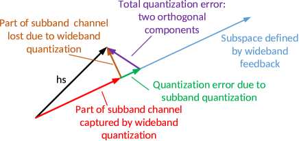
Figure 2: Quantization error partition.

Fig. 2, and the following conclusions summarize our findings of the theoretical basis for modular CSI quantization:

• Quantization performance depends on two independent parts: wideband distortion, characterized by $d_{p}(\mathbf{W},\widetilde{\mathbf{R}})$, and a subband distortion, which depends on the codebook ${\mathcal{H}}$. Improving either part improves the overall quantization (Proposition 1).

• If $\mathbf{W}$ is fixed, even perfect subband quantization does not provide perfect overall quantization due to $d_{p}(\mathbf{W},\mathbf{R})$.

• With orthogonal $\mathbf{W}$, improving subband effective channel quantization by reducing $D_{\cal B}$ directly reduces overall distortion (Corollary 1).

Note that the analysis above reveals how the subband distortion is given by the orthogonal component $\mathbf{W}$, while the singular values $\mathbf{\Sigma}$ affect the effective subband channel distortion $D_{\cal B}$.

V Wideband Quantization

We consider a situation where multiple MIMO channels are operated in parallel on subbands in the frequency domain, and the frequency-selective channels are correlated between subbands as discussed in Section II.

V-A Eigenvector Quantization

In this section we consider wideband quantization pertaining to using a budget of bits for feeding back information about the $K$ largest eigenvectors of a covariance matrix ${\mathbf{R}}$ as precisely as possible. From Proposition 1, the objective of wideband quantization is to find

$$\mathbf{W}=\arg\min_{\bar{\mathbf{W}}\in{\cal W}}\,d_{p}(\bar{\mathbf{W}},\widetilde{\mathbf{R}})$$ (33)

where $d_{p}(\bar{\mathbf{W}},\widetilde{\mathbf{R}})$ is the projection distortion (27), and ${\cal W}$ is a codebook of $N_{t}\times K$ matrices. As we are separately interested in the $K$ columns, Grassmannian codebooks [23, 28, 31, 32] of $K$-dimensional subspaces are not of interest. Also, due to the modular design in mind, the phases of the $K$ columns are irrelevant. Accordingly, codebooks of generic $N_{t}\times K$ unitary (Stiefel) matrices [30] are not of interest either. Pertinent matrix codebooks would quantize the flag manifold ones [34], i.e. Stiefel matrices modulo scalar column rotations.

We stress that in contrast to the literature [24, 26], we use the sample covariance of the normalized subband channels $\tilde{\mathbf{h}}$. According to Propostion 1, this quantity governs the contribution of wideband quantization to overall distortion.

Motivated by Lemma 1, we want to feed back information about orthonormal matrices. Orthonormality can be guaranteed by directly using a matrix codebook consisting of orthogonal matrices [23, 28, 30, 34]. To minimize the projection distortion, it is essential to have a high granularity of ${\cal W}$. If matrix codebooks of the kind of [23, 28, 30, 34] are used, high granularity leads to high complexity. In [25, 26, 27], complexity is kept at bay by using a high-granularity Grassmannian vector codebook ${\cal V}$ to quantize the eigenvectors one by one. The quantization process in [25, 26] proceeds as a series of parallel exhaustive searches for the optimal codewords each of which quantizes one column of $\mathbf{U}_{K}$:

$$\mathbf{v}_{k}=\arg\underset{\mathbf{v}\in{\cal V}}{\mathrm{min}}~{}~{}d(\mathbf{u}_{k},\mathbf{v})~{}~{}\mathrm{for}~{}k=1,2,\dots,K\,,$$ (34)

and the wideband feedback matrix becomes $\mathbf{V}=[\mathbf{v}_{1},\mathbf{v}_{2},\dots,\mathbf{v}_{K}]$. The codebook ${\cal V}$ consists of $N_{t}$-dimensional unit norm vectors, i.e. ${\cal V}\triangleq\{\hat{\mathbf{v}}_{1},\hat{\mathbf{v}}_{2},\dots,\hat{\mathbf{v}}_{2^{B}}\}$ and has cardinality $2^{B}$. The complexity of finding a codeword using (34) is the $K$th root of the complexity of finding a codeword in matrix codebook ${\cal W}$ with the same granularity. Columnwise Grassmann line quantization has the added benefit that it operates natively on the flag manifold, as opposed to a matrix Grassmann [23, 28, 31, 32] or Stiefel [30] quantization.

However, if ${\cal V}$ is overcomplete, there is a high probability that $\mathbf{V}\mathbf{V}^{\rm H}\neq\mathbf{I}_{N_{t}}$. According to Proposition 1, this breaks the connection between subband channel and effective channel quantization. Which is to say, the basis spanned by a typical $\mathbf{V}$ is probably independent but not orthogonal, which causes errors when quantizing the subband channel using $\mathbf{V}$.

Motivated by this, we develop two wideband quantization approaches, namely orthonormalized wideband precoding (OWP) and sequential wideband precoding (SWP), that improve not only the quality of wideband feedback but also the accuracy of subband channel projection—they enable high-granularity feedback of orthogonal bases, with the same complexity as (34).

V-A1 Orthonormalized Wideband Precoding (OWP)

We aim at $N_{t}\times K$ dimensional wideband feedback, using a vector codebook ${\cal V}$, and an independent quantization (34) of eigenvectors. The quantization data pertaining to the resulting $\mathbf{V}$ is fed back to the BS.

It is important to distinguish between $\mathbf{V}$ with columns in ${\cal V}$, and the orthogonal basis matrix $\mathbf{W}$ used to compute the subband feedback. We assume that the users and the BS have agreed on a method to orthonormalize the vectors $\mathbf{V}$. There is a deterministic function which produces an orthogonal $N_{t}\times K$ matrix from a generic $N_{t}\times K$ matrix, e.g. Gram-Schmidt orthogonalization;

$$\mathbf{W}=\mathrm{orth}(\mathbf{V})\,,$$ (35)

which would recover precisely the result of the QR-decomposition in (22). This method is shared at the same time as the codebook ${\cal V}$. Exactly the same number of bits can thus be used to feed back the orthogonal $\mathbf{W}$ as feeding back the original $\mathbf{V}$.

The user constructs the orthogonal $\mathbf{W}$ and uses it to compute the effective channels. The BS similarly constructs $\mathbf{W}$ from $\mathbf{V}$ and uses it as the basis in which subband feedback is interpreted.

In [28], scalar quantization is used to feed back information of a rectangular unitary matrix, and the recipient of the feedback extracts the unitary columns. The difference to OWP is that in OWP, both the user and the BS perform orthogonalization using the same orthogonalization algorithm, and the user uses the orthogonalized $\mathbf{W}$ to determine and the BS to interpret subsequent feedback.

V-A2 Sequential Wideband Precoding (SWP)

In [27], a sequential method to find codewords $\mathbf{v}\in{\cal V}$ was presented, with the objective to find the best basis $\mathbf{V}$ of $K$ vectors for $N_{t}$-dimensional vectors $\mathbf{h}$. Here, we use a similar approach to find $\mathbf{V}$ and to orthogonalize it. In [27], the equivalent channel coordinates were computed by pseudoinversion, and the BS used $\mathbf{V}$ when reconstructing the channel. In contrast, we compute the equivalent channel using the orthogonalized $\mathbf{W}$, and the BS uses $\mathbf{W}$; the users and the BS use the same orthogonalization principle.

The intuition of SWP is to provide a self-correction capability to the quantization process. The quantization of eigenvector $k$ may not only convey information about the eigenvector $\mathbf{u}_{k}$, it may also convey information about the errors of quantizing the eigenvectors $\mathbf{u}_{j}$ of higher eigenvalues $j<k$.

For this, define a projector $\mathbf{\Pi}^{\perp}$ updated in each iteration $j$, and initialized at the identity matrix. For convenience, we denote its value at iteration $j$ as $\mathbf{\Pi}^{\perp},j$, and $\mathbf{\Pi}^{\perp}_{0}={\bf I}_{N_{t}}$. This matrix characterizes the perpendicular space of all previous feedback vectors. In the $j$-th iteration we calculate the projection of the covariance matrix $\widetilde{\mathbf{R}}$ to the current perpendicular space $\mathbf{\Pi}^{\perp}_{j-1}$:

$$\widetilde{\mathbf{R}}_{j}=\mathbf{\Pi}^{\perp}_{j-1}~{}\widetilde{\mathbf{R}}~{}\mathbf{\Pi}^{\perp}_{j-1},~{}j=1,\dots,K.$$ (36)

Then the strongest eigenvalue eigenvector ${\bf e}_{j,1}$ of $\widetilde{\mathbf{R}}_{j}$ is found using, e.g., the power method. Utilizing the vector quantization codebook we then quantize ${\bf e}_{j,1}$ to $\mathbf{v}_{j}\in{\cal V}$.

Algorithm 1 Sequential Wideband Precoding (SWP)

1:  Initialization

2:      $\mathbf{\Pi}^{\perp}_{0}={\bf I}_{N_{t}}$

3:  Wideband Quantization

4:      for $j=1,2,\dots,K$ do

5:         Project $\widetilde{\mathbf{R}}$ to $\mathbf{\Pi}^{\perp}$ using (36): $\widetilde{\mathbf{R}}_{j}$

6:         Find strongest eigenvector ${\bf e}_{j,1}$ of $\widetilde{\mathbf{R}}_{j}$

7:         Quantize ${\bf e}_{j,1}$ using wideband codebook to $\mathbf{v}_{j}$

8:         Project $\mathbf{v}_{j}$ to $\mathbf{\Pi}^{\perp}$ with (37), normalize: $\mathbf{w}_{j}$

9:         Update $\mathbf{\Pi}^{\perp}$ with $\mathbf{w}_{j}$ using (38)

10:      end for

11:  Output

12:      Obtain basis matrix $\mathbf{W}=[\mathbf{w}_{1},\mathbf{w}_{2},\dots,\mathbf{w}_{K}]$

13:      Obtain feedback matrix $\mathbf{V}=[\mathbf{v}_{1},\mathbf{v}_{2},\dots,\mathbf{v}_{K}]$

Next, we project the quantized strongest eigenvector $\mathbf{v}_{j}$ to the perpendicular space of the previous codewords:

$$\tilde{\mathbf{v}}_{j}=\mathbf{\Pi}^{\perp}_{j-1}\mathbf{v}_{j},$$ (37)

and orthonormalize it to $\mathbf{w}_{j}=\tilde{\mathbf{v}}_{j,{\rm q}}/|\tilde{\mathbf{v}}_{j}|$. Finally, the perpendicular space is updated to

$$\mathbf{\Pi}^{\perp}_{j}=\mathbf{\Pi}^{\perp}_{j-1}-\mathbf{w}_{j}\mathbf{w}_{j}^{\rm H}.$$ (38)

Note that in each iteration, $\mathbf{\Pi}^{\perp}_{j}$ is a projector; $\left(\mathbf{\Pi}^{\perp}_{j}\right)^{2}=\mathbf{\Pi}^{\perp}_{j}$ and $\left(\mathbf{\Pi}^{\perp}_{j}\right)^{\rm H}=\mathbf{\Pi}^{\perp}_{j}$.

After $K$ iterations, the user feeds back the matrix $\mathbf{V}=\left[\mathbf{v}_{1},\mathbf{v}_{2},\dots,\mathbf{v}_{K}\right]$ consisting of $K$ codewords in the vector quantization codebook ${\cal V}$ to the BS. The user applies the corresponding orthogonal matrix $\mathbf{W}=\left[\mathbf{w}_{1},\mathbf{w}_{2},\dots,\mathbf{w}_{K}\right]$ when deriving subband feedback. The BS, knowing the SWP algorithm, can reproduce $\mathbf{W}$ from $\mathbf{V}$, and uses it as the basis when interpreting subband feedback.

SWP is summarized in Alg.1. When considering this as an algorithm for sequentially finding a $\mathbf{V}$, there is a crucial difference to [27]. In Alg.1, projectors act on the remainder, while in [27], projectors act separately on each codeword in ${\cal V}$ at each stage of the algorithm. This results in considerably higher computational complexity than Alg.1.

To formulate a performance measure, we need a technical characterization of codebooks. We consider covariance matrices $\widetilde{\mathbf{R}}$ with continuously distributed eigenvectors, and a codebook ${\cal V}$ quantizing vectors $\mathbf{u}$ in this distribution to points $\mathbf{v}\in{\cal V}$ that are at most at chordal distance $r$ from $\mathbf{u}$. The quantization can be characterized by the inner product $\mathbf{u}^{\rm H}\mathbf{v}$ of the normalized vectors. If the probability distribution of inner products across all $\mathbf{u}$ and their corresponding $\mathbf{v}$ does not depend on the phase of the inner product, and is a non-increasing function of the chordal distance $d(\mathbf{u},\mathbf{v})$, we call the quantization radial, and the chordal distance is the quantization error. For a more detailed discussion, see Appendix A.

Note that OWP of Section V-A1 does not reduce the projection distance as compared to using the possibly non-orthogonal $\mathbf{W}$ produced by parallel quantization in (34). OWP only produces effective channels which can be quantized based on isometry. In contrast, for SWP we have:

Proposition 2

Assume a radial codebook ${\cal V}$ for quantizing the distribution of eigenvectors of $\widetilde{\mathbf{R}}$, with maximal quantization error $r\leq 1/\sqrt{2}$. SWP of Algorithm 1 provides a smaller projection distortion than OWP of (34).

Proof:

See Appendix A. ∎

V-B Wideband Amplitude Quantization

Quantizing the real-valued singular values $\mathbf{\Sigma}$ is rather straightforward. There is a budget of bits for feeding back information about them, and scalar quantization can be directly used. With quantized $\mathbf{V}$, and especially with orthogonalized $\mathbf{W}$, the singular values computed from (3) do not characterize the relative weight of the columns in $\mathbf{W}$ when describing subbands. Instead we calculate wideband amplitudes (19) for each column $\mathbf{w}_{j}$ in $\mathbf{W}$, and feed back scalar quantized versions $\{\hat{\sigma}_{j}\}$.

VI Subband Effective Channel Quantization

Now we concentrate on quantizing subband-specific effective channel coordinates. The BS and user share a $N_{t}\times K$ wideband basis matrix $\mathbf{W}$ which reduces dimensionality of subband channels to $K$, and the quantized wideband amplitude matrix $\hat{\mathbf{\Sigma}}$. The $K$-dimensional effective channel $\mathbf{b}_{s}=\mathbf{W}^{\rm H}\mathbf{h}_{s}$ becomes (4) for perfect wideband feedback. It is not i.i.d., but according to Lemma 1 it is an isometry for orthogonal $\mathbf{W}$. The effective channel $\mathbf{c}_{s}=\hat{\mathbf{\Sigma}}^{-1}\mathbf{b}_{s}$ becomes the i.i.d. (5) for perfect wideband feedback. The squared chordal distance for the quantization is

$$d^{2}(\mathbf{h}_{s},\hat{\mathbf{h}})=1-\left|\mathbf{h}_{s}^{\rm H}\hat{\mathbf{h}}\right|^{2}=1-\left|\mathbf{b}_{s}^{\rm H}\hat{\mathbf{b}}\right|^{2}=d^{2}(\hat{\mathbf{\Sigma}}\,\mathbf{c}_{s},\,\hat{\mathbf{\Sigma}}\,\hat{\mathbf{c}})\,.$$ (39)

Thus, if quantizing $\mathbf{c}_{s}$, we should use the quantization metric (39) instead of chordal distance.

VI-A Vector Quantization from Deformed i.i.d. Codebook

Following [12, 9], an i.i.d. vector quantization codebook ${\cal C}$ may be deformed with $\hat{\mathbf{\Sigma}}$ to ${\cal B}$ of (20), which is then used to quantize $\mathbf{b}_{s}$, minimizing (39). Even with a relatively small $K$, the precision required from the i.i.d. codebook ${\cal C}$ may be prohibitive for applying full-fledged vector quantization. We shall use product codebooks (PCB) [14, 15, 16] with a trellis structure based on $N_{\ell}<K$ -dimensional component codes. With $N_{b}$ bits per component, we use $N_{t}/N_{\ell}\times N_{b}$ bits in total. To deform the quantization according to [12, 9], we incorporate $\hat{\mathbf{\Sigma}}$ to the trellis metric in a blockwise manner, corresponding to the component code being processed.

VI-B Scalar Quantization with Adaptive Bit Allocation

As an alternative, scalar quantization of the entries of $\mathbf{c}_{s}$ may be applied, with adaptive bit-allocation derived from $\hat{\mathbf{\Sigma}}$. Further simplification can be achieved by separately quantizing phase and amplitude [35]. Scalar quantization has the benefit that large codebooks can be used with limited quantization complexity, as quantization is coordinate by coordinate. The normalized subband effective channel $\mathbf{c}$ is a $K\times 1$ i.i.d. vector $\mathbf{c}=[c_{1},c_{2},\dots,c_{K}]^{\rm T}$. As overall phase is irrelevant, one of the coordinates acts as phase reference. The objective is to minimize (39).

VI-B1 Bit Allocation in Extrinsic Order

In 5G NR [25, 26], quantization bit allocation is based on the order of singular values $\hat{\sigma_{i}}$. This ordering is extrinsic to the effective channel coordinates $c_{i}$. The coordinate $c_{\max}$ with largest $\sigma_{i}$ is used as phase and amplitude reference. For $m$ the coordinates with the next largest $\sigma_{j}$, $c_{j}/c_{\max}$ are uniformly quantized in phase with $B_{\ell}$ bits and in amplitude with one bit to $\{1,1/\sqrt{2}\}$. The power ratio in the codebook is thus $\eta=2$. For the remaining $K-(m+1)$ coordinates, amplitudes are quantized to $1/\sqrt{2}$ (no bits), while $B_{s}<B_{\ell}$ bits are used for the phases. The number of bits used for quantizing $\mathbf{c}$ is thus $L=(B_{\ell}+1)m+B_{s}(K-m-1)$.

VI-B2 Bit Allocation in Intrinsic Order

Starting from first principles we develop an adaptive bit allocation principle taking the sizes of $c_{j}$ into account. Accordingly, this scheme is based on an intrinsic order. When using coordinate-specific codebooks ${\cal C}_{i}$ divided to separate amplitude and phase parts, the crucial observations to make from (16,39) are that effective channel coordinates $c_{i}$ are fading $\mathcal{CN}(0,1)$ random variables; as they are i.i.d., their quantizations should have the same mean energy $E_{\hat{c}_{i}\in{\cal C}_{i}}\left\{|\hat{c}_{i}|^{2}\right\}=a^{2}$; subject to this, the weighted inner product $\left|\mathbf{c}^{\rm H}\hat{\mathbf{\Lambda}}\,\hat{\mathbf{c}}\right|=\sum_{j=1}^{K}\,\hat{\sigma}_{j}^{2}\,|c_{j}^{*}\hat{c}_{j}|$ should be maximized. The contribution of $\hat{c}_{j}$ to feedback error depends on the weighted amplitude $\hat{\sigma}_{j}|c_{j}|$. Following these principles we first normalize $\mathbf{c}$, and then quantize all amplitudes with one bit. Assuming perfect phase quantization, for Rayleigh fading variables the optimum quantization levels have a power ratio of $\eta\approx 5$, see [36]. Denoting the quantized amplitude of coordinate $c_{i}$ as $\hat{a}_{i}$, we use $\alpha_{i}=\hat{\sigma}_{i}\,\hat{a}_{i}$ to order the coordinates for phase bit allocation. The coordinate with largest $\alpha_{i}$ is used as phase reference. To the coordinates with the $m$ next largest $\alpha_{i}$, we allocate $B_{\ell}$ phase bits, while to the $K-(m+1)$ coordinates with smallest $\alpha_{i}$, we allocate $B_{s}$ phase bits. The total number of subband quantization bits required becomes: $L=K+B_{\ell}\,m+B_{s}(K-m-1)$.

TABLE I: Quantization methods simulated

Fig.	Quant. problem	distortion metric	CB	Benchmark
5	WB vector	chordal	TSODFT, DD	TSODFT
5	WB matrix	projection	TSODFT, DD	TSODFT
			OWP, SWP	OWP
			${\bf R}_{B00B}$, ${\bf R}_{B+B-},{\bf R}$	$\mathbf{R}$
7	Subband	chordal	PCB, INT5, EXT2	EXT2
7,9	Overall	chordal	IND, OWP, SWP	IND
	quantization		PCB, INT5, EXT2	EXT2
			TSODFT, ${\bf R}_{B00B}$
9	MU-MIMO ZF	Spec. Eff.	IND+EXT2, OWP+INT5, SWP+INT5	IND+EXT2
			TSODFT, ${\bf R}_{B00B}$

VII Simulations

The simulation results are organized as follows: Sec.VII-B-Sec.VII-D show the results of wideband, subband and overall quantization in order, as summarized in Table I. We compare the quantization performance of different methods and select superior methods (in red) for subsequent comparisons.

VII-A Settings and Schemes

For simulating the developed modular CSI quantization scheme, we need a channel model with a realistic combination of channel directivity and frequency domain correlation, as well as a realistic model of an mMIMO antenna array.

VII-A1 Channel Model

The BS has a Uniform Planar Array (UPA) with $N_{t}=32$ antennas, divided into $8\times 2\times 2$ horizontal $\times$ vertical $\times$ polarization elements, depicted in Fig. 3. The center frequency is $1.84$ GHz and the bandwidth is $18$ MHz with $1200$ subcarriers divided into $S=30$ subbands. We use QuaDRiGa V2.0.0 [37] to generate MIMO channels with 3GPP 38.901 UMa NLOS settings, assuming $8$ scattering clusters and a ratio of 80% indoor users.

We model a 120-degree sector of a base station, and 1000 single-antenna users are dropped uniformly at random within 250 m from the BS in the sector. Users have omnidirectional antennas, and as we only take users in one sector, BS antennas are considered omnidirectional as well. For each user, the covariance matrix $\widetilde{\mathbf{R}}$ is found by averaging over subbands.

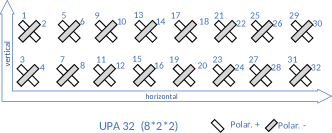
Figure 3: ($8\times 2\times 2$)-element UPA diagram illustration.

VII-A2 Polarization Decomposition of Channel

With the UPA antenna arrangement of Fig. 3 the subband channel vector $\mathbf{h}$ is a 3D Kronecker product [38]:

$$\mathbf{h}=\mathbf{h}_{h}\otimes\mathbf{h}_{v}\otimes\mathbf{h}_{p}\,.$$

Here $\mathbf{h}_{h},\mathbf{h}_{v},\mathbf{h}_{p}$ denote the horizontal, vertical and polarization parts with $8,2,2$ elements, respectively. The channel covariance matrix $\widetilde{\mathbf{R}}$ and the wideband codebook for $\mathbf{W}$ are correspondingly decomposed.

Different polarizations of BS antennas are weakly correlated within a sector, see [39]. This can be used to reduce feedback pertaining to $\widetilde{\mathbf{R}}$. We rearrange the channel vectors into $\mathbf{h}^{\rm T}=[\mathbf{h}_{+}^{\rm T},\,\mathbf{h}_{-}^{\rm T}]$, according to the $+/-$ polarization. In addition to quantizing the fully-occupied covariance matrices, we consider two reduced alternatives assuming weak cross-polarization correlation. The correlations of the two polarizations are assumed either the same, or different:

$${\bf R}_{B+B-}=\left[\begin{array}[]{ll}\mathbf{B}_{+}&\bf 0\\ \bf 0&\mathbf{B}_{-}\end{array}\right]~{}{\rm or}~{}~{}{\bf R}_{B00B}=\left[\begin{array}[]{cc}\mathbf{B}&\bf 0\\ \bf 0&\mathbf{B}\end{array}\right]\,.$$ (40)

Here $\mathbf{B}$, $\mathbf{B}_{+}$ and $\mathbf{B}_{-}$ are $N_{t}/2\times K/2$ matrices, and $\mathbf{B}=(\mathbf{B}_{+}+\mathbf{B}_{-})/2$. In simulations, the $K=8$ strongest eigenvectors of $\widetilde{\mathbf{R}}$ are used, while for $\mathbf{B}$, $\mathbf{B}_{+}$, or $\mathbf{B}_{-}$, the $K/2=4$ strongest are quantized.

VII-A3 Wideband Quantization

For quantizing the covariances arising in the three polarization partition methods above, we apply

• IND: the standardized method used in [25] where wideband vectors are independently quantized; $\mathbf{W}$ and $\hat{\mathbf{\Sigma}}$ are direct quantizations of $\mathbf{U}$ and $\mathbf{\Sigma}$ from (3).

• OWP: $\mathbf{W}$ is orthogonalized, wideband amplitudes are (19) and effective channels (17).

• SWP: $\mathbf{W}$ is orthogonalized with Alg.1.

The singular values or wideband amplitudes $\{\sigma_{j}\}$ are scalar quantized. The strongest beam is indicated and the amplitudes of the remaining $K-1$ beams are quantized by $3$ bits each using the codebook $\{1/\sqrt{2^{m}}\}_{m=0}^{6}\cup\{0\}$ from [25].

VII-A4 Wideband Vector Quantization Codebooks

Following [26, 27] we apply array architecture aware precoding for UPA. We decompose wideband vector codebooks as ${\cal V}_{h}\otimes{\cal V}_{v}\otimes{\cal V}_{p}$, where ${\cal V}_{h},{\cal V}_{v}$ and ${\cal V}_{p}$ quantize the horizontal, vertical and polarization dimensions, respectively. We use oversampled DFT codebooks for ${\cal V}_{h}$ and ${\cal V}_{v}$ in respective dimensions, resulting in a Tensored Oversampled DFT (TSODFT) codebook. In the fully-occupied case, for ${\cal V}_{p}$ we use a $2$-bit binary chirp (BC) codebook [40], which is an ideal i.i.d. codebook of this size.

We also use data-driven (DD) Grassmann quantization codebooks, found by applying the Lloyd algorithm to a training set of eigenvectors of wideband covariance matrices. Compared with random vector codebooks, data-driven Grassmann quantization codebooks take the distribution of data samples to be quantized into account, reducing distortion.

VII-A5 Subband Quantization Codebooks

For subband feedback, we use the options

• Correlated vector quantization based on a product codebook, denoted as PCB

• Adaptive scalar quantization with extrinsic order and power ratio $\eta=2$, denoted as EXT2

• Adaptive scalar quantization with intrinsic order and power ratio $\eta=5$, denoted as INT5

PCB is discussed in Section VI-A, and the scalar quantizations in Section VI-B.

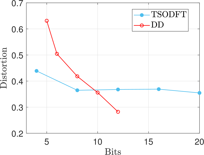
Figure 4: Wideband vector codebook distortion. Tensored Oversampled DFT (TSODFT) vs. Data Driven (DD) codebooks.

5

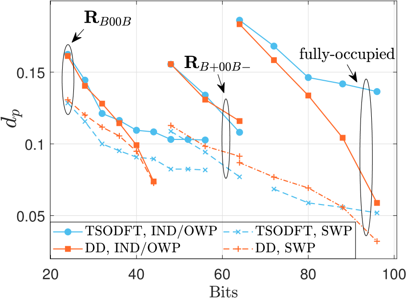
Figure 5: Wideband matrix projection distortion. Four combinations of codebooks (TSODFT or DD) and matrix quantization principles (OWP or SWP) for different dolarization decompositions.

VII-B Wideband Quantization Performance Comparison

VII-B1 Vector Quantization Distortion w.r.t. $\mathbf{u}_{k}$

We first compare the wideband vector quantization codebooks used for quantizing the $K=8$ strongest eigenvectors $\mathbf{u}_{k}$ of sample covariance matrices. In Fig. 5 we see that with smaller numbers of bits, the array architecture aware TSODFT codebook performs better than the data driven one, while with increasing numbers of bits, the DD codebook is able to learn the distribution of the eigenvectors, resulting in smaller distortion.

VII-B2 Projection Distortion w.r.t. $\widetilde{\mathbf{R}}$

We compare OWP and SWP w.r.t. the projection distortion (33) under three polarization structures, ${\bf R}_{B00B}$, ${\bf R}_{B+B-}$ od (40), and the fully-occupied $\bf R$, for TSODFT and DD codebooks.

In Fig. 5, each of the twelve combinations is simulated for several codebook sizes, and projection distortion is reported against the total number of bits. Recalling that the projection distortion $d_{p}$ does not depend on orthogonalization, the same distortion arises for OWP and independent vector quantization IND, while SWP may have different $d_{p}$. In Fig. 5, SWP outperforms IND/OWP for all polarization structures, which agrees with Proposition 2. In most cases the gap between SWP and IND/OWP is large. When the number of bits increases, saturation can be observed for TSODFT, in accordance with Fig. 5. Interestingly, when the number of bits increases, OWP and SWP converge for DD. The reason is that when the data driven approach starts to learn an appropriate quantization for the eigenvectors of the channels, the gain provided by SWP in correcting quantization errors for the largest eigenvectors reduces.

Polarization structure ${\bf R}_{B00B}$ provides the best trade-off between performance and codebook cardinality. Fully-occupied SWP yields the lowest $d_{p}$, at the cost of twice the number of bits. We focus on ${\bf R}_{B00B}$ and TSODFT below due to easy implementation and good performance.

VII-C Subband Quantization Performance Comparison

We compare subband quantization schemes in terms of the distortion $D_{{\cal B}}$ of subband effective channel quantization. Here, a subtle effect comes into play. A given $\widetilde{\mathbf{R}}$ has singular values $\mathbf{\Sigma}$, with a spread $\sigma_{\max}-\sigma_{\min}$. The correlation structure $\hat{\mathbf{\Sigma}}$ of subband quantization, however, depends on the wideband quantization scheme. With wideband quantization precision decreasing, the spread of $\hat{\mathbf{\Sigma}}$ decreases and the volume of the subband effective channel space $\mathbf{W}^{\rm H}\mathbf{h}_{s}$ and the corresponding distortion $D_{{\cal B}}$ increases. In Fig. 7 we consider $D_{\cal B}$ with ideal wideband quantization and with OWP. EXT2 and INT5 based on scalar quantization with bit allocation, as well as correlated PCB are considered. PCB performs the best followed by INT5 while EXT2 is the worst. Hence, we focus more on comparing INT5 and PCB below. In OWP with smaller singular value spread than with ideal wideband quantization, INT5 almost catches up with PCB. For SWP, the $D_{\cal B}$-values would be closer to the ideal case, while for IND, considering $D_{\cal B}$ does not make sense as the independently quantized $\mathbf{V}$ is not an isometry of chordal distance.

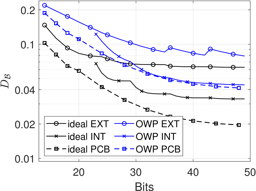
Figure 6: Subband codebook distortion with ideal wideband quantization, and with OWP, for subband codebooks EXT, INT and PCB.

5

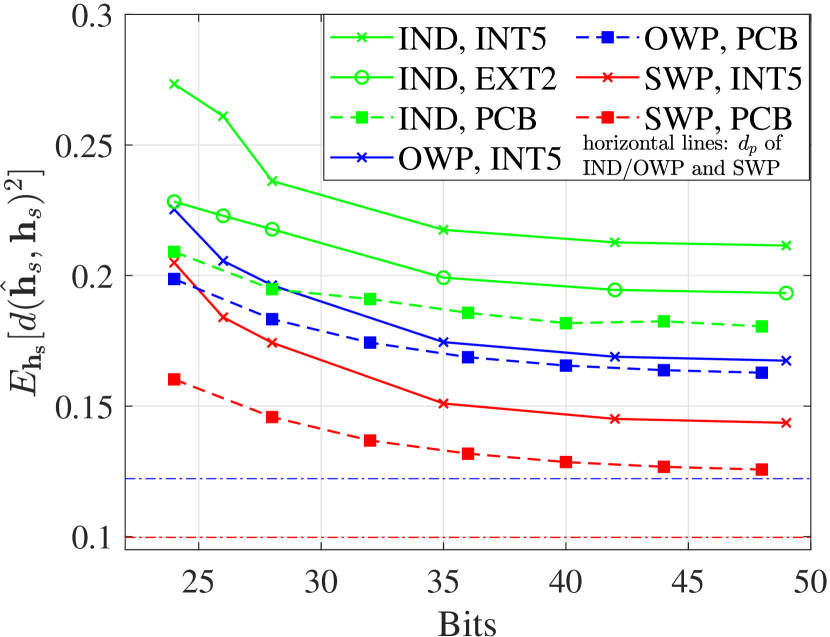
Figure 7: Overall distortion comparison. Combinations of wideband matrix quantization principles (IND,OWP,SWP) and subband codebooks (INT5,EXT2,PCB) for WB vector codebook TSODFT, and polarization structure ${\bf R}_{B00B}$.

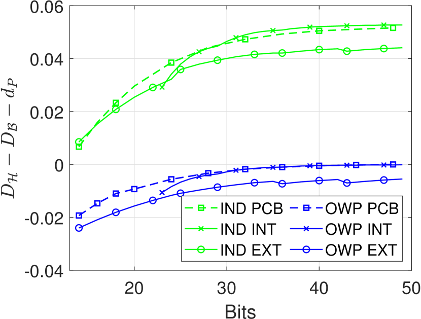
Figure 8: Difference between total distortion $D_{\mathcal{H}}$ and upper bound $D_{\cal B}+d_{p}$ of Corollary 1, valid for orthogonal wideband feedback (OWP).

5

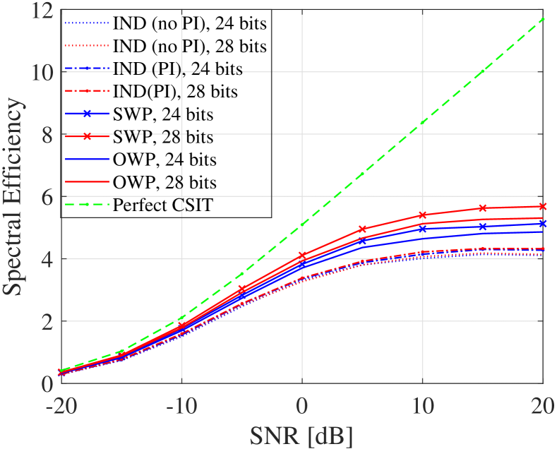
Figure 9: Multiuser scenario: Spectral efficiency with 4 users: SWP, OWP and IND with/without pseudoinversion (PI).

VII-D Overall Quantization Distortion

Next we consider the overall quantization distortion $D_{\mathcal{H}}=E_{\mathbf{h}_{s}}[d(\hat{\mathbf{h}}_{s},\mathbf{h}_{s})^{2}]$. For OWP and SWP wideband feedback we consider INT5 and PCB, according to Fig. 7. For independent wideband quantization we consider all three subband quantization schemes, EXT2, INT5 and PCB. TSODFT with over-sampling ratio $\omega=16$ is used for polarization structure ${\bf R}_{B00B}$.

The resulting overall distortion vs. the number of bits for subband quantization is reported in Fig. 7. For OWP, the performance difference between PCB and INT5 is fully captured by the subband performance in Fig. 7, in concordance with Corollary 1. The gain of PCB is enhanced when combined with SWP, and for both OWP and SWP, the total distortion is lower bounded by the corresponding projection distortion, in line with Proposition 1 and Corollary 1. For OWP and SWP are $d_{p}=0.122$ and $0.01$, respectively, plotted with dashed lines. For IND, EXT2 outperforms IND5, as expected from [25]. PCB, however, outperforms EXT2 also for IND.

To verify the validity of the upper bound in Corollary 1, we have plotted the difference between the overall subband channel distortion $D_{\mathcal{H}}$ and the upper bound $D_{\cal B}+d_{p}$ in Fig. 9, for OWP and IND. Subband effective channel distortion $D_{\cal B}$ is calculated for the actual distribution of subband channels arising for a given wideband channel quantization, e.g., for OWP with PCB and INT, the $D_{\cal B}$ from Fig. 7 are used. As OWP is based on orthogonal wideband feedback, Corollary 1 holds, and accordingly we see that the difference is $\leq 0$. For IND, the corollary does not hold—we see that for non-orthogonal wideband feedback, the channel distortion $D_{\mathcal{H}}$ may be much larger than what would be expected based on the part of the channel projected out, $d_{P}$, and the subband effective channel distortion, $D_{\cal B}$.

VII-E Multiuser Spectral Efficiency

To understand the effects of finite granularity modular CSI feedback on communication rate, we evaluate performance in a multiuser scenario with $M=4$ single antenna users. The subcarriers are divided into $S=25$ subbands each with $48$ subcarriers. All users are simultaneously served in the subbands. Based on CSI fed back from the individual users, the BS performs zero forcing (ZF) precoding on each subband. The three wideband quantization schemes from Section VII-A3 are compared, with their respective best subband quantization with 24 and 28 bits. All users are assumed to have the same SNR. As a benchmark, ZF spectral efficiency with perfect channel state information at Tx is considered.

Average single user spectral efficiency $R=\log_{2}(1+\gamma)$ with $\gamma$ the ZF-SINR of a user is plotted vs. SNR in Fig. 9. Simulations corroborate the theoretical principles discussed of sections IV-C and V. OWP outperforms independent quantization by more than 25%, while SWP outperforms OWP by more than 8%. Only nominal gain is achieved if users apply pseudoinversion to compute the coordinates with independent quantization, while the BS uses $\mathbf{V}$. Increasing the effective channel quantization granularity improves OWP and SWP considerably, while providing little gain for independent quantization, confirming the distortion result in Fig. 7.

VIII Conclusions

We have addressed modular CSI quantization for massive MIMO systems. Analyzing the separation of feedback to a dimensionality reducing wideband part and a lower-dimensional subband part, we found quantization objectives for optimal modular quantization. We show considerable performance improvement in a mMIMO scenario when applying these principles. An orthonormalized wideband precoding (OWP) scheme and a sequential wideband precoding (SWP) scheme are developed. Sharing a wideband feedback orthogonalization principle between the transmitter and receiver makes it possible to accurately quantize the lower-dimensional subbands. Without shared orthogonalization, improved subband quantization is not guaranteed to improve overall quantization accuracy.

It is worth noting that our central result, Proposition 1, holds for any situation where processing of a vector is divided to two stages, where in the first stage the vector is dimensionality reduced to a subspace, and where the quality of the processing is measured by the chordal distance. Accordingly, this result readily generalizes to CSI feedback in a situation with multiple Rx antennas. This also extends the applicability of our results to mainstream Time Division Duplexing mMIMO, e.g. to front-hauled distributed processing for mMIMO, especially in the cell-free mMIMO case.

Appendix

VIII-A Proof of Proposition 2

We first prove a needed lemma, and its corollary. We investigate quantization codebooks ${\mathcal{H}}$ in the space of unit norm $N_{t}$-dimensional complex vectors $\mathbf{u}$ modulo phase, i.e., the Grassmann manifold ${\cal G}_{\mathbb{C}}(N_{t},1)$. The chordal distance (14) is a metric on the Grassmannian. For properties of metric balls, as well as geometric and coding properties of the Grassmannian, see [5, 41].

The vectors $\mathbf{u}$ are quantized to a $\mathbf{v}\in{\cal V}$ belonging to the Voronoi cell $V(\mathbf{v})$. A metric ball $B(\mathbf{v},r)$ with radius $r$ centered at $\mathbf{v}$ consists of all $\mathbf{u}$ with $d(\mathbf{u},\mathbf{v})\leq r$. To simplify the analysis we assume radially distributed quantization errors; the probability density of quantization error vectors of an arbitrary $\mathbf{u}$ is rotationally invariant and non-increasing in error magnitude. This means that the direction and magnitude of the quantization error are independent random variables, and the distribution may be, e.g., uniform. There is a maximum quantization error given by ${\mathcal{H}}$, s.t. the quantization errors are distributed in a ball $B(\mathbf{u},r)$. We have:

Lemma 2

Consider quantization of a source vector $\mathbf{u}\in{\cal G}_{\mathbb{C}}(N,1)$ to a $\mathbf{v}$ radially distributed in the ball $B(\mathbf{u},r)$. Projecting and normalizing $\mathbf{u}$ to an $m$-dimensional subspace yields $\mathbf{u}_{\rm s}$, with $|\mathbf{u}^{\rm H}\mathbf{u}_{\rm s}|^{2}={1-\epsilon^{2}}$ for an $\epsilon\leq\sqrt{1-r^{2}}$, while projecting and normalizing $\mathbf{v}$ results in $\mathbf{v}_{\rm s}$. The normalized projection $\mathbf{v}_{\rm s}$ is radially distributed in a ball with radius $r/\sqrt{1-\epsilon^{2}}$, centered at $\mathbf{u}_{\rm s}$, and with the mean $\mathbf{u}_{\rm s}$. Denoting the quantization error after projection as $d=d(\mathbf{u}_{\rm s},\mathbf{v}_{\rm s})$, with the conditional distribution $f_{D|E}(d|\epsilon)$, for any $\epsilon>0$ there is a crossover quantization error $d_{c}$ such that $f_{D|E}(d|0)>f_{D|E}(d|\epsilon)$ for $d<d_{c}$, and $f_{D|E}(d|0)<f_{D|E}(d|\epsilon)$ for $d>d_{c}$.

Proof:

Vector $\mathbf{u}$ is fixed. Take a point $\mathbf{v}\in B(\mathbf{u},r)$. As we are interested in chordal distance, all vectors are Grassmannian, i.e., they are equivalent under overall phase rotations. We decompose $\mathbf{u}$ and $\mathbf{v}$ to components in the projection subspace and its complement as

$$\mathbf{u} = \epsilon\,\mathbf{u}_{\bf o}+\sqrt{1-\epsilon^{2}}\,\mathbf{u}_{\rm s}$$ (41)

$$\mathbf{v} = \alpha\,\mathbf{v}_{\bf o}+\sqrt{1-\alpha^{2}}\,\mathbf{v}_{\rm s}$$ (42)

Here, $\mathbf{u}_{\rm s}$, $\mathbf{u}_{\bf o}$, $\mathbf{v}_{\rm s}$ and $\mathbf{v}_{\bf o}$ are all unit norm vectors, and $\epsilon$ and $\alpha$ represent the fraction of the vectors projected out.

Now fix $\mathbf{v}_{\rm s}$ with $\left|\mathbf{u}_{\rm s}^{\rm H}\mathbf{v}_{\rm s}\right|=\cos\theta$ for some $\theta\in[0,\pi/2]$. For each $\mathbf{v}_{\rm s}$ there is a preimage of vectors $\mathbf{v}\in B(\mathbf{u},r)$ that project to $\mathbf{v}_{\rm s}$. It follows from the Cauchy-Schwarz inequality that

$$\mathbf{b}=\frac{1}{\nu}\left(\epsilon\,\mathbf{u}_{\bf o}+\sqrt{1-\epsilon^{2}}\,\cos\theta\,\mathbf{v}_{\rm s}\right)$$ (43)

is the closest vector to $\mathbf{u}$ in this preimage. Here the normalization is

$$\nu=\sqrt{\epsilon^{2}+\cos^{2}\!\theta(1-\epsilon^{2})}\,.$$ (44)

The preimage isomorphic to a set of unit vectors up to overall phase in $N-m+1$ dimensions, i.e. ${\cal G}_{\mathbb{C}}(N-m+1,1)$. For concreteness, the basis vectors can be taken as $\mathbf{u}_{\rm o},\mathbf{v}_{\rm s}$ together with $N-m-2$ null-vectors of the projection orthogonal to $\mathbf{u}_{\rm o}$. The projection maps all of these vectors to $\mathbf{v}_{\rm s}$. All vectors $\mathbf{a}$ in the preimage should have $|\mathbf{u}^{\rm H}\mathbf{a}|^{2}\geq 1-r^{2}$. It follows again from Cauchy-Schwarz that the vectors in the preimage with largest chordal distance to $\mathbf{b}$ are $\mathbf{a}_{\max}=\beta\mathbf{b}+\mathbf{b}_{\rm o}$, where $\beta=\sqrt{(1-r^{2})/\nu^{2}}$, and $\mathbf{b}_{\rm{}_{o}}$ is orthogonal to $\mathbf{u}_{\rm o}$ and $\mathbf{v}_{\rm s}$. These vectors are at chordal distance

$$r_{\nu}=\sqrt{1-(1-r^{2})/\nu^{2}}$$ (45)

from $\mathbf{b}$. The preimage is thus an $N-m+1$-dimensional ball $B(\mathbf{b},r_{\nu})$ centered at $\mathbf{b}$. It is easy to convince oneself that the preimages of all $\mathbf{v}_{\rm s}$ are distinct, recalling that the overall phases of both $\mathbf{v}$ and $\mathbf{v}_{\rm s}$ are irrelevant.

For a given $\epsilon$ there exists a smallest $\theta$ for which the ball has non-negative radius, $\theta_{\min}=\arccos\sqrt{(1-\epsilon^{2}-r^{2})/(1-\epsilon^{2})}$, leading to a maximal chordal distance between projections:

$$d^{2}(\mathbf{u}_{\rm s},\mathbf{v}_{\rm s})\leq r_{{\rm s}}=\frac{r}{\sqrt{1-\epsilon^{2}}}~{}.$$ (46)

The probability density at $\mathbf{v}_{\rm s}$ is an integral over the preimage $B(\mathbf{b},r_{\nu})$. For any $\mathbf{v}_{\rm s}$ at fixed distance from $\mathbf{u}_{\rm s}$, i.e. fixed $\theta$, the geometry and the probability density in the preimage are the same. The probability of $\mathbf{v}_{\rm s}$ thus only depends on $d(\mathbf{u}_{\rm s},\mathbf{v}_{\rm s})$; we have $f(\mathbf{v}_{\rm s})\sim f_{\Theta|E}\left(\arccos\left(|\mathbf{v}_{\rm s}^{\rm H}\mathbf{u}_{\rm s}|\right)|\epsilon\right)$ for some $f_{\Theta|E}(\theta|\epsilon)$.

Now, from (43) and (45) we see that, for fixed $\epsilon$ the radius of $B(\mathbf{b},r_{\nu})$ decreases with $\theta$, while the distance of $\mathbf{b}$ from $\mathbf{u}_{\rm o}$ grows. The ball always has a point with maximum chordal distance $r$ from $\mathbf{u}$, which has the smallest probability density, while the probability density at the center, $\mathbf{b}$, decreases with $\theta$. Furthermore, the integration measure in the preimage decreases with increasing $\alpha$ as $\sqrt{1-\alpha^{2}}$. The attenuation due to the integration measure thus increases with distance from $\mathbf{u}_{\rm o}$ in ${\cal G}_{\mathbb{C}}(N-m+1,1)$. As a consequence, the probability of $\mathbf{v}_{\rm s}$ decreases monotonically with $\theta$. The larger $\theta$ is, the smaller a ball is integrated over, the smaller are the probability densities in the preimage integrated over, and the larger is the attenuation $\sqrt{1-\alpha^{2}}$ due to the integration measure. Accordingly, the probability distribution of $\mathbf{v}_{\rm s}$ is radial, centered at $\mathbf{u}_{\rm s}$, and thus averaging to $\mathbf{u}_{\rm s}$.

To complete the proof, the distributions for different $\epsilon$ have to be addressed. At $\theta=0$, the factor $\sqrt{1-\alpha^{2}}$ in the integration measure decreases with $\epsilon$. Thus $f_{\Theta|E}(0,\epsilon)$ monotonically decreases with $\epsilon$. With increasing $\theta$, the radius to integrate over in the preimage grows with $\epsilon$. As a consequence, if $f_{\Theta|E}(\theta_{1},\epsilon_{1})>f_{\Theta|E}(\theta_{1},\epsilon_{2})$ for $\epsilon_{1}<\epsilon_{2}$, we also have $f_{\Theta|E}(\theta_{2},\epsilon_{1})>f_{\Theta|E}(\theta_{2},\epsilon_{2})$ for $\theta_{2}<\theta_{1}$. For $\theta>r$, $f_{\Theta|E}(\theta,0)=0$, while for $\epsilon>0$, there is probability mass in a range of $\theta>r$, according to (46). ∎

Corollary 2

Consider arbitrary projections $\mathbf{\Pi}$ of a positive semi-definite matrix $\mathbf{R}$, with an ensemble of radial quantizations ${\cal V}$ of the eigenvectors such that the quantization $\mathbf{v}$ of $\mathbf{u}$ is in a ball $B(\mathbf{u})$ with radius $r\leq 1/\sqrt{2}$. The expected Rayleigh Quotient (RQ) $E_{\mathbf{v}\in B(\mathbf{u})}\left\{{\mathbf{v}^{\rm H}\mathbf{\Pi}\mathbf{R}\,\mathbf{\Pi}\mathbf{v}}/{\mathbf{v}^{\rm H}\mathbf{\Pi}\mathbf{v}}\right\}$ is maximized for $\mathbf{u}$ the largest eigenvector $\mathbf{e}$ of $\mathbf{\Pi}\mathbf{R}\mathbf{\Pi}$.

Proof:

The eigenvector $\mathbf{e}$ lies in the projected space, thus Lemma 2 holds for it with $\epsilon=0$, while for an arbitrary $\mathbf{u}$, generically $\epsilon>0$. Denote the quantizations of these $\hat{\mathbf{e}}$ and $\hat{\mathbf{u}}$. From the lemma, the distribution of $\mathbf{\Pi}\hat{\mathbf{e}}$ is in a $B_{e}$ centered at $\mathbf{e}$ with quantization error distribution $f_{0}(\theta)$, while $\mathbf{\Pi}\hat{\mathbf{u}}$ is in $B_{u}$ centered at $\mathbf{\Pi}\mathbf{u}$ with a larger radius and a wider distribution $f_{\epsilon}(\theta)$.

The RQ is generically non-convex, but in a ball with chordal distance radius $1/\sqrt{2}$ around the largest eigenvector $\mathbf{e}$ it is convex. $B_{e}$ lies in this convexity region. Moreover, for any great circle going through $\mathbf{e}$, the value of the quotient on the circle at any point outside this ball is less than the values of the circle within this ball. The same holds for the circle arising from rotating any point in this ball in the plane spanned by the two largest eigenvectors. Applying this in reverse order to each eigendirection except $\mathbf{e}$, one may rotate $B_{u}$ to be centered at $\mathbf{e}$. As the probability distribution is radial, the expectation of the RQ does not decrease. Finally, by changing the distribution from $f_{\epsilon}$ to $f_{0}$, the expectation again does not decrease due to the great circle property. ∎

Now we are equipped for proving Proposition 2.

Proof:

As orthogonalization of $\mathbf{W}$ does not affect its projection metric, for OWP we compare the projection distortion of a $\mathbf{W}$ created using QR-decomposition of the form (22) on the feedback matrix $\mathbf{V}$, resulting in an upper triangular $\mathbf{C}$.

For both OWP and SWP we have orthogonal $N_{t}\times K$ -matrices $\mathbf{W}$ with columns $\mathbf{w}_{j}$. Their $N_{t}\times j$ submatrices are denoted by $\mathbf{W}_{j}=\left[\mathbf{w}_{1},\ldots,\mathbf{w}_{j}\right]$, and the corresponding projectors (37) to perpendicular spaces are $\mathbf{\Pi}^{\perp}_{j}=\mathbf{I}-\mathbf{W}_{j}\mathbf{W}_{j}^{\rm H}$. The projection distortion can be decomposed as

$$d_{p}(\mathbf{W},\widetilde{\mathbf{R}})=1-\sum_{j=1}^{K}\mathbf{w}_{j}^{\rm H}\widetilde{\mathbf{R}}\mathbf{w}_{j}\,.$$ (47)

In both OWP and SWP, $\mathbf{w}_{j}$ is selected by quantizing an eigenvector with the closest vector in a vector codebook ${\cal V}$. In SWP, the resulting codeword is explicitly projected by $\mathbf{\Pi}^{\perp}_{j-1}$ and normalized. In OWP with upper triangular $\mathbf{C}$, exactly the same happens. Thus both for SWP and OWP, the projection distortion can be characterized as

$$d_{p} = 1-\sum_{j=1}^{K}\mu_{j}(\mathbf{v}_{j})$$ (48)

$$\mu_{j}(\mathbf{v}) = \frac{\mathbf{v}^{\rm H}\mathbf{\Pi}^{\perp}_{j-1}\widetilde{\mathbf{R}}\mathbf{\Pi}^{\perp}_{j-1}\mathbf{v}}{\mathbf{v}^{\rm H}\mathbf{\Pi}^{\perp}_{j-1}\mathbf{v}}~{},$$ (49)

where $\mu_{j}$ is a Rayleigh Quotient (RQ) of $\widetilde{\mathbf{R}}$ in the subspace projected by $\mathbf{\Pi}_{j-1}$. For fixed $\mathbf{W}_{j-1}$ and infinite granularity, the RQ would be maximized by the largest eigenvector $\mathbf{e}_{j,1}$ of $\mathbf{\Pi}^{\perp}_{j-1}\widetilde{\mathbf{R}}\mathbf{\Pi}^{\perp}_{j-1}$. With a finite granularity codebook ${\cal V}$, we consider three candidate codewords:

$$\mathbf{v}_{\max} = \arg\max{}_{\mathbf{v}\in{\cal V}}~{}\mu_{j}(\mathbf{v})$$ (50)

$$\mathbf{v}_{\perp} = \arg\min{}_{\mathbf{v}\in{\cal V}}~{}d(\mathbf{e}_{1,j},\mathbf{v})$$ (51)

$$\mathbf{v}_{u} = \arg\min{}_{\mathbf{v}\in{\cal V}}~{}d(\mathbf{u}_{j},\mathbf{v})\,.$$

The first by definition minimizes the contribution of $\mathbf{w}_{j}$ to the projection distortion, given the previous vectors $\mathbf{W}_{j-1}$. Finding it would require computing the RQ for each element in ${\cal V}$. The second, $\mathbf{v}_{\perp}$ is the result of steps 7-8 in Algorithm 1, while $\mathbf{v}_{u}$ is the codeword selected in OWP before orthogonalization.

By construction $\mu_{j}(\mathbf{v}_{\max})\geq\mu_{j}(\mathbf{v}_{\perp})$ and $\mu_{j}(\mathbf{v}_{u})$. From Corollary 2, we have $E_{\widetilde{\mathbf{R}}}\left\{\mu_{j}(\mathbf{v}_{\perp})\right\}\geq E_{\widetilde{\mathbf{R}}}\left\{\mu_{j}(\mathbf{v}_{u})\right\}$. As $\mathbf{u}$ comes from a continuous distribution, however, equality has probability 0.

Now compare the projection distortion as a sum (48) over quantized codewords $\mathbf{v}_{j}$ for OWP and SWP. After $j$ terms have been summed, the projector for OWP is $\widetilde{\mathbf{\Pi}}_{j}$ and the one for SWP $\mathbf{\Pi}_{j}$. The expectation of the remaining terms for OWP, $\sum_{k=j+1}^{N}\mu_{k}(\mathbf{v}_{k})$ does not change if $\widetilde{\mathbf{\Pi}}_{j}$ is replaced with $\mathbf{\Pi}_{j}$. The reason for this is that the difference between $\mathbf{\Pi}_{j}$ and $\widetilde{\mathbf{\Pi}}_{j}$ on the remaining eigenvectors $\mathbf{u}_{k}$ for $k>j$ is due to differences in quantization errors, which produce the same result on average. Considering this after each $j$ in the sum (48) completes the proof. ∎

References

- [1] R. Vehkalahti, J. Liao, T. Pllaha, W. Han, and O. Tirkkonen, “CSI quantization for FDD massive MIMO communication,” in IEEE VTC Spring, 2021, pp. 1–5.
- [2] H. Q. Ngo, E. G. Larsson, and T. L. Marzetta, “Energy and spectral efficiency of very large multiuser MIMO systems,” IEEE T. Commun., vol. 61, no. 4, pp. 1436–1449, 2013.
- [3] J. Hamalainen and R. Wichman, “Closed-loop transmit diversity for FDD WCDMA systems,” in Proc. Asilomar Conf., vol. 1, 2000, pp. 111–115.
- [4] D. J. Love, R. W. Heath, and T. Strohmer, “Grassmannian beamforming for multiple-input multiple-output wireless systems,” IEEE T. Inf. Th., vol. 49, no. 10, pp. 2735–2747, 2003.
- [5] W. Dai, Y. Liu, and B. Rider, “Quantization bounds on Grassmann manifolds and applications to MIMO communications,” IEEE T. Inf. Th., vol. 54, no. 3, pp. 1108–1123, 2008.
- [6] N. Jindal, “MIMO broadcast channels with finite-rate feedback,” IEEE T. Inf. Th., vol. 52, no. 11, pp. 5045–5060, 2006.
- [7] W. Lee, I. Sohn, B. O. Lee, and K. B. Lee, “Enhanced unitary beamforming scheme for limited-feedback multiuser MIMO systems,” IEEE Commun. Lett., vol. 12, no. 10, pp. 758–760, 2008.
- [8] A. Adhikary, J. Nam, J. Ahn, and G. Caire, “Joint spatial division and multiplexing—the large-scale array regime,” IEEE T. Inf. Th., vol. 59, no. 10, pp. 6441–6463, 2013.
- [9] P. Xia and G. B. Giannakis, “Design and analysis of transmit-beamforming based on limited-rate feedback,” IEEE T. Sign. Proc., vol. 54, no. 5, pp. 1853–1863, 2006.
- [10] J. Roh and B. Rao, “Transmit beamforming in multiple-antenna systems with finite rate feedback: a VQ-based approach,” IEEE T. Inf. Th., vol. 52, no. 3, p. 1101 –1112, 2006.
- [11] V. Raghavan and R. W. Heath and A. M. Sayeed, “Systematic codebook designs for quantized beamforming in correlated MIMO channels,” IEEE J. Select. Areas Commun., vol. 25, no. 7, pp. 1298–1310, 2007.
- [12] D. J. Love and R. W. Heath, “Limited feedback diversity techniques for correlated channels,” IEEE T. Veh. Tech., vol. 55, no. 2, pp. 718–722, 2006.
- [13] Y. Cheng, V. Lau, and Y. Long, “A scalable limited feedback design for network MIMO using per-cell product codebook,” IEEE T. Wirel. Commun., vol. 9, no. 10, pp. 3093 –3099, October 2010.
- [14] F. Yuan and C. Yang, “Bit allocation between per-cell codebook and phase ambiguity quantization for limited feedback coordinated multipoint transmission systems,” IEEE T. Commun., vol. 60, no. 9, p. 2546–2559, Sep. 2012.
- [15] C. K. Au-Yeung, D. J. Love, and S. Sanayei, “Trellis coded line packing: Large dimensional beamforming vector quantization and feedback transmission,” IEEE T. Wirel. Commun., vol. 10, no. 6, pp. 1844–1853, 2011.
- [16] J. Choi and D. J. Love and T. Kim, “Trellis-extended codebooks and successive phase adjustment: A path from LTE-advanced to FDD massive MIMO systems,” IEEE T. Wirel. Commun., vol. 14, no. 4, pp. 2007–2016, 2015.
- [17] R.-A. Pitaval and O. Tirkkonen, “Joint Grassmann-Stiefel quantization for MIMO product codebooks,” IEEE T. Wirel. Commun., vol. 13, no. 1, pp. 210–222, 2014.
- [18] D. Gunduz and P. Kerret and & al., “Machine learning in the air,” IEEE J. Select. Areas Commun., vol. 37, no. 10, pp. 2184–2199, 2019.
- [19] M. Mashhadi, Q. Yang, and D. Gunduz, “Distributed deep convolutional compression for massive MIMO CSI feedback,” IEEE T. Wirel. Commun., vol. 20, no. 4, pp. 2621–2633, 2021.
- [20] T. Wang, C. K. Wen, J. Shi, and G. Y. Li, “Deep Learning-Based CSI Feedback Approach for Time-Varying Massive MIMO Channels,” IEEE Wireless Commun. Lett., vol. 8, no. 2, pp. 416–419, 2019.
- [21] J. Nam, A. Adhikary, J. Y. Ahn, and G. Caire, “Joint spatial division and multiplexing: Opportunistic beamforming user grouping and simplified downlink scheduling,” IEEE J. Sel. Topics Sign. Proc., vol. 8, no. 5, pp. 876–890, Oct. 2014.
- [22] J. Chen and V. K. N. Lau, “Two-tier precoding for FDD multi-cell massive MIMO time-varying interference networks,” IEEE J. Select. Areas Commun., vol. 32, no. 6, pp. 1230–1238, 2014.
- [23] S. Ghosh, B. D. Rao, and J. R. Zeidler, “Techniques for MIMO channel covariance matrix quantization,” IEEE T. Sign. Proc., vol. 60, no. 6, pp. 3340–3345, 2012.
- [24] Y. Liu, G. Y. Li, and W. Han, “Quantization and feedback of spatial covariance matrix for massive MIMO systems with cascaded precoding,” IEEE T. Commun., vol. 65, no. 4, pp. 1623–1634, 2017.
- [25] Samsung et. al, “WF on Type I and II CSI codebooks,” 3GPP, Tech. Rep. R1-1709232, 2017.
- [26] E. Onggosanusi & al., “Modular and high-resolution channel state information and beam management for 5G New Radio,” IEEE Commun. Mag., vol. 56, no. 3, pp. 48–55, 2018.
- [27] J. Song, J. Choi, T. Kim, and D. J. Love, “Advanced quantizer designs for FDD-based FD-MIMO systems using uniform planar arrays,” IEEE T. Sign. Proc., vol. 66, no. 14, pp. 3891–3905, 2018.
- [28] S. Schwarz, M. Rupp, and S. Wesemann, “Grassmannian product codebooks for limited feedback massive MIMO with two-tier precoding,” IEEE J. Select. Topics Sign. Proc., vol. 13, no. 5, pp. 1119–1135, 2019.
- [29] D. Sacristan-Murga, M. Payaro, and A. Pascual-Iserte, “Transceiver design framework for multiuser MIMO-OFDM broadcast systems with channel Gram matrix feedback,” IEEE T. Wirel. Commun., vol. 11, no. 5, pp. 1774–1787, 2012.
- [30] S. Schwarz and M. Rupp, “Tree-structured quantization on Grassmann and Stiefel manifolds,” in 2021 Data Compression Conference (DCC), 2021, pp. 303–312.
- [31] ——, “Reduced complexity recursive Grassmannian quantization,” IEEE Sign. Proc. Lett., vol. 27, pp. 321–325, 2020.
- [32] S. Schwarz and T. Tsiftsis, “Codebook training for trellis-based hierarchical Grassmannian classification,” IEEE Wireless Commun. Lett., vol. 11, no. 3, pp. 636–640, 2022.
- [33] E. Landau, Einführung in die Differential- und Integralrechnung. Groningen: P. Noordhoff N.V., 1934.
- [34] R.-A. Pitaval, A. Srinivasan, and O. Tirkkonen, “Codebooks in flag manifolds for limited feedback MIMO precoding,” in ITG Conf. on Systems, Commun. and Coding (SCC), 2013, pp. 1–5.
- [35] A. Dowhuszko and J. Hämäläinen, “Performance of transmit beamforming codebooks with separate amplitude and phase quantization,” IEEE Sign. Proc. Lett., vol. 22, no. 7, 2015.
- [36] W. Pearlman, “Polar quantization of a complex Gaussian random variable,” IEEE T. Commun., vol. 27, no. 6, pp. 892–899, 1979.
- [37] Fraunhofer Heinrich Hertz Institute, “The implementation of quasi deterministic radio channel generator (QuaDRiGa) v2.0.0,” https://quadriga-channel-model.de/.
- [38] D. Ying, F. W. Vook, T. A. Thomas, D. J. Love, and A. Ghosh, “Kronecker product correlation model and limited feedback codebook design in a 3d channel model,” in 2014 IEEE international conference on communications (ICC). IEEE, 2014, pp. 5865–5870.
- [39] J. Hamalainen and R. Wichman, “On correlations between dual-polarized base station antennas,” in Proc. IEEE GLOBECOM, vol. 3, 2003, pp. 1664–1668.
- [40] S. D. Howard, A. R. Calderbank, and S. J. Searle, “A fast reconstruction algorithm for deterministic compressive sensing using second order Reed-Muller codes,” in Conf. Information Sciences and Systems, Mar. 2008, pp. 11–15.
- [41] R.-A. Pitaval, L. Wei, O. Tirkkonen, and C. Hollanti, “Density of spherically embedded Stiefel and Grassmann codes,” IEEE T. Inf. Th., vol. 64, no. 1, 2018.