What is a degree of freedom?

Abstract

Understanding degrees of freedom is fundamental to characterizing physical systems. Counting them is usually straightforward, especially if we can assign them a clear meaning. For example, a particle moving in three-dimensional space has three degrees of freedom, one for each independent direction of motion. However, for more complex systems like spinning particles or coupled harmonic oscillators, things get more complicated since there is no longer a direct correspondence between the degrees of freedom and the number of independent directions in the physical space in which the system exists.

This paper delves into the intricacies of degrees of freedom in physical systems and their relationship with configuration and phase spaces. We first establish the well-known fact that the number of degrees of freedom is equal to the dimension of the configuration space, but show that this is only a local description. A global approach will reveal that this space can have non-trivial topology, and in some cases, may not even be a manifold. By leveraging this topology, we gain a deeper understanding of the physics. We can then use that topology to understand the physics better as well as vice versa: intuition about the configuration space of a physical system can be used to understand non-trivial topological spaces better.

1 Introduction

Perhaps the most basic question that one can ask about a physical system is: how can it change? In some cases, this is obvious. A roller coaster on a track can move either forwards or backwards. This system has a single degree of freedom (DOF): there is only one way in which it can change. Further, this DOF is physically manifest, simply corresponding to the position of the roller coaster on the track. In many other cases, the DOFs are not so obvious. Consider a hockey puck moving around an ice rink and assume that it stays flat to the surface. Further, assume that it has been battered by extended use and so no longer has a perfect rotational symmetry. Hence one can distinguish between its various rotated states. There are two manifest DOFs associated with the position of its centre of gravity. However, there is also a rotational DOF which specifies its angle of rotation around that centre of gravity. Hence the puck has three DOFs. Already in this example, things have become significantly more complicated than for the roller coaster. The positional DOFs are no longer uniquely specified: any pair of (non-parallel) directions would be sufficient. Further, the rotational DOF is associated with an angle rather than a location. Vaguely one might think that this is because we can specify the rotation angle with a single number, and this is partly right but not the full story.

To see this, move up to three dimensions. The puck has now been hit hard and left the ice, tumbling as it travels through the air. There are then three DOFs associated with its position in three-dimensional space. Working in analogy from the one-dimensional spin, one might naively expect there to be two directions of rotational freedom. After all, using spherical coordinates, it only takes two angles to specify the position on the surface of a sphere. However, this is not correct and confuses the orientation of an axis with rotations around at axis. There are three rotational DOFs: two angles to specify the orientation of the axis running through the center of the puck and a third one to specify the rotation angle around that axis. Hence, there are now six degrees of freedom, and again, they could equally well be associated with any coordinate system and any way of specifying orientation and angle of rotation.

Aside from the issue of identifying DOFs, it is also clear that not all DOFs are created equal. For example, a roller coaster running on a linear track differs from one running around a closed track. In the first case, to return to the starting point, the train has to go back over the track it previously traversed. However, in the second case, it can also return simply by continuing in the same direction. In both cases, there is one local DOF, but globally there is a difference. Similarly, for the puck, rotating by $360^{\circ}$ around any axis returns it to its original state, but no amount of spatial translation in a single direction will return it to its original location. These highlight the difference between a DOF and the configuration space or C-space. The C-space is the set of all possible inequivalent states that a system can take. The C-space of the roller coaster is the set of all positions along the track. For the on-ice hockey puck, it is all locations in the rink along with all possible orientations. Finally, for the puck tumbling through the air, the C-space is the location of the (centre of gravity) of the puck along with all orientations of the spin axis and rotations around that axis.

Though they are distinct, there is obviously a very close relationship between DOFs and the C-space: the former enumerates the number of ways one can independently move through the latter. However, there is more to DOFs and C-space than just that relationship, and one of the main goals of this article is to understand these ideas better. To that end, in Section 2, we begin by considering how they apply in multiple physical systems, including ones with an infinite number of degrees of freedom. We start to develop a mathematical understanding of the C-space as a differentiable manifold. Then in Section 3, which is the bulk of the paper, we cement this understanding, focusing on double pendulum systems of various types. We see how their C-spaces can have non-trivial topologies, including those of the torus, Klein bottle, and Möbius strip. We then focus on the specific example of mechanical linkages (these can be thought of as a pair of double pendulums which share a common bob) and use them to construct many examples of physical systems with two DOFs but whose C-spaces have an even wider range of topologies. We classify them using triangulations and the Euler characteristic. We finish the paper with an example of a mechanical system with one DOF whose C-space is not a manifold.

2 Configuration space, phase space and degrees of freedom

This section studies the C-spaces of various physical systems in more detail. It also considers more carefully the relationship between a system’s C-space and its physics. We begin with point particles.

2.1 Classical point particles

Many problems in introductory physics start with a particle (or another object) moving in a straight line. The possible positions of the particle, its C-space, are fully described by a single number $x\in\mathbb{R}$, so there is a single DOF. However, there is more to physics than just the C-space: a one-dimensional particle can exhibit many different types of physics. For example, it could be a harmonic oscillator or a particle rolling down an inclined plane under the effect of gravity, but the C-space (the statics) remains the same. Physics is added to the C-space by specifying a force $f$ in Newton’s second law:

$$f(x)=ma=m\ddot{x}\;.$$ (1)

In that case, the C-space is not sufficient to fully specify the state of the system in the future. We need to know the position and the velocity of the particle. This is so because (1) is a (time-independent) second-order ordinary differential equation. Thus, we need a good set of initial conditions $(x_{o},v_{o}$). Another way to describe the initial condition is using the phase space: a typical element being $(x,p)$ where $p=mv$ is the momentum. In terms of the phase space, the Newton equations become the coupled first-order equations:

$$m\dot{x}=p\quad\mbox{and}\quad\dot{p}=f(x)\;.$$ (2)

As a concrete example, consider the one-dimensional simple harmonic oscillator. Then, we have

$$\ddot{x}=-kx\quad\Longleftrightarrow\qquad m\dot{x}=p\quad\mathrm{and}\quad\dot{p}=-mkx\,,$$ (3)

for some positive constants $m$ (mass) and $k$ (spring constant), where $x$ represents the displacement from the equilibrium point. Assuming an ideal system, $x$ can take any value in the real line, so the C-space is $\mathcal{C}^{\mathrm{HO}}_{1}=\mathbb{R}$. Further, the velocity can take any value, and so the phase space is $\mathcal{P}^{\mathrm{HO}}_{1}=\mathbb{R}\times\mathbb{R}$. Notice that the choice of coordinates to describe the DOF is not unique. For example, instead of distance $x$ from a point, we could describe its position with $y=e^{x}$. In that case, $y\in\mathcal{C}^{\mathrm{HO}}_{2}:=(0,\infty)$ which fully specifies the configuration. From a static perspective, these choices of C-space are equivalent (diffeomorphic), but from a dynamical perspective, the equations of motion using $x\in\mathcal{C}^{\mathrm{HO}}_{1}$ are simpler to write and solve than using $y\in\mathcal{C}^{\mathrm{HO}}_{2}$. Whatever manipulations we impose, there is a single DOF: the number of parameterizing coordinates remains the same.

Following the simple harmonic oscillator, perhaps the second most common example in physics is the planar pendulum: a pendulum for which the bob is fixed at the end of a rigid (massless) bar. Then the C-space is the circle $\mathcal{C}_{1}^{\mathrm{PP}}=\mathbb{S}^{1}$ and, as for the simple harmonic oscillator, there is a single DOF. However, the description of that DOF is more complicated. For the oscillator, we can specify the location with a single number $x\in\mathbb{R}$ and there is a one-to-one relationship between the location and the numbers describing the location. For the pendulum, things are not so simple as the configuration space is topologically different from $\mathbb{R}$. The best that we can do is map part of $\mathbb{R}$ onto part of $\mathbb{S}^{1}$. For example, we can describe its position with the angle $\theta$ from the vertical axis so it can take the values $\theta\in[0,2\pi)$. However, distinguishing the zero by placing it on the boundary of our domain is inconvenient, so let us explore other options. We could consider $\theta\in(-\pi,\pi)$, and whenever we need to cover the north pole, we change to another variable $\theta^{\prime}\in(0,2\pi)$. Then we need two sets of numbers to cover all the states. Yet another option would be to take $(x,y)\in\mathbb{R}^{2}$ representing the position of the end of the pendulum. These numbers are subject to the constraint $x^{2}+y^{2}=\ell^{2}$ where $\ell$ is a fixed number representing the pendulum’s length. In this case we have two coordinates $(x,y)$ but also a constraint between them, so the number of independent coordinates (DOFs) remains $2-1=1$. Finally, another equivalent option would be to assume $\theta\in\mathbb{R}$ and identify $\theta$ and $\theta+2\pi k$ for every $k\in\mathbb{Z}$. This last option is actually the most convenient for our purposes. The C-space would then be the quotient space $\mathbb{R}/(2\pi\mathbb{Z})$, which is, as Figure 1 suggests, equivalent to the circle $\mathbb{S}^{1}$.

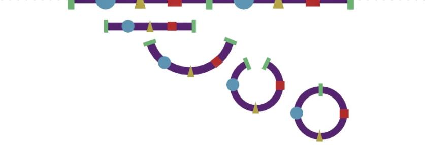
Figure 1: By identifying $x\sim x+2\pi$ in $\mathbb{R}$, we end up with one cut $[0,2\pi]$ in which the endpoints are identified. Gluing those endpoints leads to a circle.

The next examples are generalizations of the previous two: the two-dimensional harmonic oscillator and the spherical pendulum. For the former, we could use coordinates $(x,y)\in\mathbb{R}^{2}$, while for the latter, we could either take several patches in spherical coordinates or three coordinates $(x,y,z)\in\mathbb{R}^{3}$ subject to the condition $x^{2}+y^{2}+z^{2}=\ell^{2}$ (three variables and two constraints, so the number of independent variables is $3-1=2$). Their C-spaces are $\mathbb{R}^{2}$ and $\mathbb{S}^{2}$, and in both cases, there are two DOFs.

So far, all these examples have a direct and obvious correspondence between the physical world and the abstract C-space. It is, however, essential to remember the distinction between them. An easy example where this correspondence is less direct is provided by two distinct particles on a plane. Each one can be described by $(x_{i},y_{i})$ and the C-space is

$$\mathcal{C}^{\mathrm{2P}}=\{(x_{1},y_{1},x_{2},y_{2})\in\mathbb{R}^{4}\ |\ (x_{1},y_{1})\neq(x_{2},y_{2})\}\;.$$

One can also consider $N$ particles moving in three dimensions. Such $N$-body problems may be relatively small (describing the motion of the planets around the Sun) or huge (simulating the motion of millions of point galaxies in a cosmological model). In three dimensions, each particle requires three numbers to describe its position, and so, the C-space is $\mathbb{R}^{3N}$ (for simplicity, we ignore the constraint that no two particles occupy the same location). Again, if particle motion is governed by second-order differential equations, then the phase space is double the size $(\mathbb{R}^{3}\times\mathbb{R}^{3})^{N}$ with the typical elements being $(x_{i},p_{i})$ for $i\in\{1,\ldots,N\}$, a position and momentum for each particle. If these particles are physical bodies that rotate, then the number of DOFs will increase further. We now consider such extended bodies.

2.2 Extended Bodies

We begin with the C-space of a scalene triangle in a three-dimensional background space. Once we understand these, extending those transformations to other examples, such as tumbling hockey pucks, will be easy. To specify the position of a scalene triangle in space, it is sufficient to fix the coordinates of its three vertices $v_{i}:=(x_{i},y_{i},z_{i})$, $i\in\{1,2,3\}$, subject to the constraints that the distance $\mathrm{d}(v_{i},v_{j})$ between $v_{i}$ and $v_{j}$ is some fixed length $\ell_{ij}$. Then

$$\mathcal{C}^{\mathrm{Tri}}_{1}=\{(v_{1},v_{2},v_{3})\in\mathbb{R}^{9}\ |\ \mathrm{d}(v_{i},v_{j})=\ell_{ij}\}\;.$$

The number of DOFs can be calculated as in the earlier examples as the difference between the number of specified pieces of information and the number of constraints: in this case, $9-3=6$.

How does this square with our earlier discussion of the hockey puck as having 3 translational DOFs and 3 rotational DOFs? To understand that, attach an orthonormal frame to our triangle. Then the position and orientation of the triangle are fully specified if we fix the position and orientation of the frame. The position of $v_{1}$ is specified by a vector $\mathbf{w}\in\mathbb{R}^{3}$, which can be thought of as a translation from the origin. Intuitively, as for the hockey puck, the orientation of the $\{\mathbf{e}_{i}\}$ frame is specified by two angles fixing the direction of $\mathbf{e}_{1}$ and then one fixing the angle of rotation of $\mathbf{e}_{2}$ and $\mathbf{e}_{3}$ around $\mathbf{e}_{1}$.

Alternatively, consider forming a $3\times 3$ matrix $A$ with the $\{\mathbf{e_{i}}\}$. As they are orthonormal, it necessarily satisfies $A^{T}\!A=I$ and by construction (as in the footnote) we can also ensure that $\mathrm{det}A=1$. Then $A$ is an orthonormal matrix, i.e., $A\in SO(3)$. This is the rotation matrix that brings the frame (and triangle) into the correct position. Thus, we have shown that the C-space of the triangle can be described as

$$\mathcal{C}^{\mathrm{Tri}}_{2}=\{(A,\mathbf{w})\in SO(3)\times\mathbb{R}^{3}\}\;.$$

Since the dimension of $SO(n)$ is $\frac{1}{2}n(n-1)$, $\mathcal{C}^{\mathrm{Tri}}_{2}$ is determined by $\frac{3}{2}(3-1)+3=6$ numbers with no constraints, as expected. In fact, this C-space is the same for any rigid body that has no symmetries. This includes our battered hockey puck. For a more obviously non-symmetric object see Figure 2.

Figure 2: We can track the rotation of any rigid body by attaching a frame and rotating it.

The phase space of a non-symmetric extended body is then the 12-dimensional $(SO(3)\times\mathbb{R}^{3})\times\mathbb{R}^{6}$. Six degrees of freedom from the configuration space, and then there are six ways that these can change in time: three translation velocities, two angular velocities specifying how the axis of rotation is changing, and one additional angular velocity specifying how fast it is rotating around that axis of rotation.

2.3 Finite dimensional configuration spaces (robot arms)

The previous rigid body considerations also allow us to understand the configuration space of a robot arm like that shown in Figure 3.

Figure 3: An artist’s concept of Canadarm3, Canada’s smart robotic system, located on the exterior of the Lunar Gateway, a small space station in orbit around the Moon [1].

At the simplest level, a robot arm can be thought of as a set of linked (and jointed) segments. To the first approximation (ignoring self-intersections), the configuration space of an arm with $n$ segments is:

• Two-dimensions: For an arm restricted to move in a plane, each joint has the freedom to point in any direction. The configuration space is

  $$\mathcal{C}^{\mathrm{arm}}_{\mathrm{2D}}=(\mathbb{S}^{1})^{n}\;.$$

  If the arm is fixed at one end, then knowing the orientation of each joint is sufficient to fully specify the position of the arm.

• Three-dimensions: For an arm allowed to move in three dimensions, we can consider two types of joints. An idealized universal joint allows the joints to assume any orientation with the associated joints pointing in any direction relative to each other. The configuration space for such a joint is $\mathbb{S}^{2}$. An idealized spherical joint also allows the segments to rotate and so has a configuration space of $SO(3)$. Then an arm with $n_{1}$ universal and $n_{2}$ spherical joints has configuration space

  $$\mathcal{C}^{\mathrm{arm}}_{\mathrm{3D}}=(\mathbb{S}^{2})^{n_{1}}\times SO(3)^{n_{2}}\;.$$

Of course, for a realistic arm, things are much more complicated [2]. Among other things, joints are not ideal, and the arm cannot self-intersect. Thus, this configuration space (also known as the joint space in robotics) is reduced. Note, too, that if one is only interested in the possible positions of the working end of the arm (which picks things up, paints, drills, or does anything else), then a kind of freedom exists in these systems: multiple arm configurations will often correspond to a particular end position. The work space is defined as the set of all possible positions that can be reached by the working end of the arm. These ideas of C-space/joint space versus reachable/work space will show up again in later sections.

2.4 Infinite dimensional configuration spaces (field theories)

The C-spaces of classical field theories such as fluid mechanics, electromagnetism, or gravity are infinite dimensional with a value (scalar) or values (vector, tensor, or spinor) for the field at each point in the space over which it is defined. Moreover, there might be some constraints on those values (not only smoothness assumptions on the field, but also physical constraints from the field equations). For more details on the mathematics of infinite-dimensional configuration spaces see, for example, [3]. Here we just do a quick overview via a couple of examples.

Just as the physics of particles was defined by second-order differential equations (through Newton’s second law), the physics of standard field theories comes from second-order partial differential equations. Like in classical mechanics, the “position” in the C-space is insufficient to fully describe the physics of the system. Good initial conditions also require knowledge of how the field is initially changing in time. We could consider, for instance, the phase space that adds a momentum field to describe the system fully.

As a first example of an infinite-dimensional C-space, consider vacuum general relativity in $(3+1)$-form used in numerical relativity. Then, the C-space consists of all spacelike Riemannian metric $h_{ij}$ defined over some three-dimensional manifold $\Sigma$ (essentially an “instant” in time). The time-evolution equations for general relativity are second order, so the phase space consists of $h_{ij}$ along with conjugate momenta $P^{ij}$. As in classical mechanics, the $P^{ij}$ are closely related to the time derivatives of the spatial metrics. Geometrically, they are related to the extrinsic curvature of the time-slices in spacetime. However, there are further complications for the configuration and phase space of general relativity: besides the equations of motion, there are also constraint equations. That means that not all regions of the phase space are physically accessible. Moreover, there is a gauge freedom which, in this case, means that there can be different coordinate representations of the same solutions. Although these issues are too complicated to discuss here (see [4] for an accessible introduction), many of them appear in the more familiar physics of electromagnetism, and so we examine their role there.

One might initially consider the C-space of electromagnetism to consist of two arbitrary vector fields: the electric field $\mathbf{E}$ and the magnetic field $\mathbf{B}$. However, with the imposition of the Maxwell equations, these fields are constrained (in the absence of charges and currents) to be divergence-free:

$$\begin{array}[]{l}\nabla\cdot\mathbf{E}=0\\ \nabla\cdot\mathbf{B}=0\end{array}$$ (4)

with coupled time evolutions

$$\begin{array}[]{l}\dot{\mathbf{E}}=\nabla\times\mathbf{B}\\ \dot{\mathbf{B}}=-\nabla\times\mathbf{E}\end{array}$$ (5)

Using standard vector calculus properties, one can check that these evolution equations preserve the constraints (4) in time.

While one could take $(\mathbf{E},\mathbf{B})$ as configuration variables, as we have seen, they are constrained relative to each other. This complication can be partially removed by working instead with the scalar and vector potentials $(\Phi,\mathbf{A})$. The magnetic field can then be defined as

$$\mathbf{B}=\nabla\times\mathbf{A}\;.$$ (6)

which automatically satisfies $\nabla\cdot\mathbf{B}=0$. This simplifies the C-space: here, $\mathbf{A}$ is unconstrained. The electric field $\mathbf{E}$, on the other hand, shows up as the conjugate momentum to $\mathbf{A}$, but is still required to be divergence-free (a constraint on the phase space). The evolution equations (5) are re-expressed in a form analogous to (2) as

$$\begin{array}[]{l}\dot{\mathbf{A}}=-\mathbf{E}-\nabla\Phi\\ \dot{\mathbf{E}}=\nabla^{2}\mathbf{A}+\nabla(\nabla\cdot\mathbf{A})\;.\end{array}$$ (7)

Notice that $\Phi$, the Coulomb potential, is freely specified and carries the gauge freedom of the problem. That means that the physically relevant fields, $\mathbf{E}$ and $\mathbf{B}$, are independent of the choice of $\Phi$.

Apart from the constraints that the fields of a C-space might have to satisfy, there can also be topological complications that split the C-space into regions which are (assuming continuity) mutually inaccessible. We first illustrate this with a simple example and then return to electromagnetism. Consider a C-space consisting of all closed strings wrapped around a cylinder (see Fig. 4). For each possible state of the string, we can count the number of times it wraps around the cylinder. Regardless of the physics we impose on the theory, assuming that the loop does not break, such a number cannot change. This is a topological invariant of the solution.

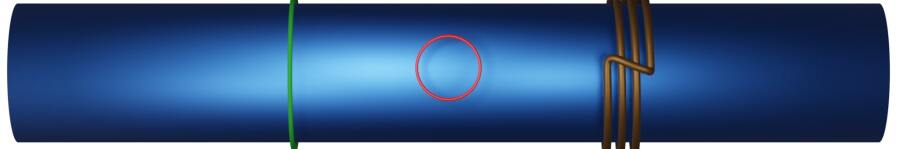
Figure 4: A cylinder with three loops: the green one (left) loops once around the cylinder, the red one (middle) wraps zero times, and the brown one (right) wraps thrice. Any continuous deformation of a loop preserves its wrapping number.

Something similar happens in electromagnetism defined over $M=\mathbb{R}^{3}\setminus\{(0,0,0)\}$ ($\mathbb{R}^{3}$ without the origin, so it is topologically nontrivial). One may construct field configurations with a magnetic charge that lives, in some sense, in the singular origin. The vector potential can be “wrapped” around the singularity analogously to the loop wrapped around the cylinder. In fact, just as the loop had an integer number of wrappings and no continuous deformation of the fields can change it, the magnetic charge is also discrete and preserved by continuous deformations of the fields (including dynamical evolutions). Like the wrappings of the loop, these magnetic monopoles are examples of topological charges. While standard charges in physics (like energy, linear and angular momentum, or electric charge) are determined by symmetries of the equations, these are instead fixed by the topology of the fields and background space. This is not a specific feature of electromagnetism, and analogous cases can be found for other gauge theories (see, for example, [5]).

3 Manifolds as Configuration Spaces of Physical Systems

The examples of the previous section have been chosen to guide the reader to the following conclusion: the C-space is actually a differentiable manifold that admits different (equivalent) representations depending on the chosen coordinate system. As for every manifold, coordinates are only valid locally, and often several coordinate patches (charts) are required to cover the whole manifold. All this implies that, in essence, a DOF can be understood as a coordinate in the C-space! On the one hand, that means that counting DOFs is very easy. We only have to check the dimension of the C-space

$$\#\mathrm{DOFs}:=\mathrm{dim}(\mathcal{C})\;.$$

In particular, for finite-dimensional C-spaces, we can simply count the number of variables $n$, the number of constraints $r$, and obtain $\#\mathrm{DOFs}=n-r$.

On the other hand, the fact that the DOFs are just coordinates (something that, of course, has been known since Lagrange started to study C-spaces) means that, in general, it does not make sense to ask “what” is a DOF or “where” it is, as those questions do not make sense for coordinates. Obviously, for concrete examples, some meaning can be given to them (e.g., they can represent time, a radial distance, or an angle), but not in general. This might seem to end our paper since there is no way to answer the very question of the title, but of course, there is still much to say. In the remainder of the paper, we are going to explore some of the nuances of this topic by studying in detail simple mechanical devices whose C-spaces are topologically non-trivial. We will finish this discussion by constructing an example where the C-space is $1$-dimensional but not exactly a manifold.

3.1 Double pendulum

An ideal double pendulum consists of a planar pendulum of length $L$ to which we attach, at the unfixed end $m$, another planar pendulum of length $\ell$ (hence $m$ becomes the middle point). Since the position of each pendulum is independent, we need one coordinate for each one, e.g., the angle $\theta_{i}\in\mathbb{S}^{1}$ with the vertical direction. Thus, as we saw when considering robot arms, the C-space is $\mathbb{S}^{1}\times\mathbb{S}^{1}$.

Topologically, $\mathbb{S}^{1}\times\mathbb{S}^{1}$ is a torus, and there is a nice visual demonstration of this fact. Consider a double pendulum in which the two planes of the movement are perpendicular to each other. Further, assume

that we have a red light at $m$ and a blue one at $p$, the end of the second pendulum. If we now take a long exposure photograph while we move the double pendulum over all possible positions, the result would be a blue torus with a red circle in the interior, proving that, in fact, the C-space is a torus. There is a little caveat with this approach: if $L=\ell$, the torus is degenerate as the hole collapses to a point (the so-called horn torus, see Fig. 5(b)). However, the C-space is still the same abstract torus, but this particular “naive” immersion does not portray it correctly. Actually, if $L<\ell$, then the torus would even intersect itself leading to the so-called spindle torus (see Fig. 5(c)). One must understand, though, that the self-intersections are not happening in the system but are an artifact of our way to immerse our C-space in $\mathbb{R}^{3}$. This is analogous to what happens when we immerse a Klein bottle in $\mathbb{R}^{3}$: an “artificial” self-intersection appears (see Fig. 5(d)). However, in that case, the situation is even worse since there exists no immersion of a Klein bottle in $\mathbb{R}^{3}$ without self-intersections.

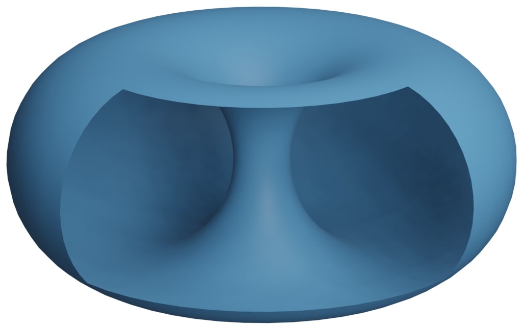
(a) $L>\ell$. Regular torus

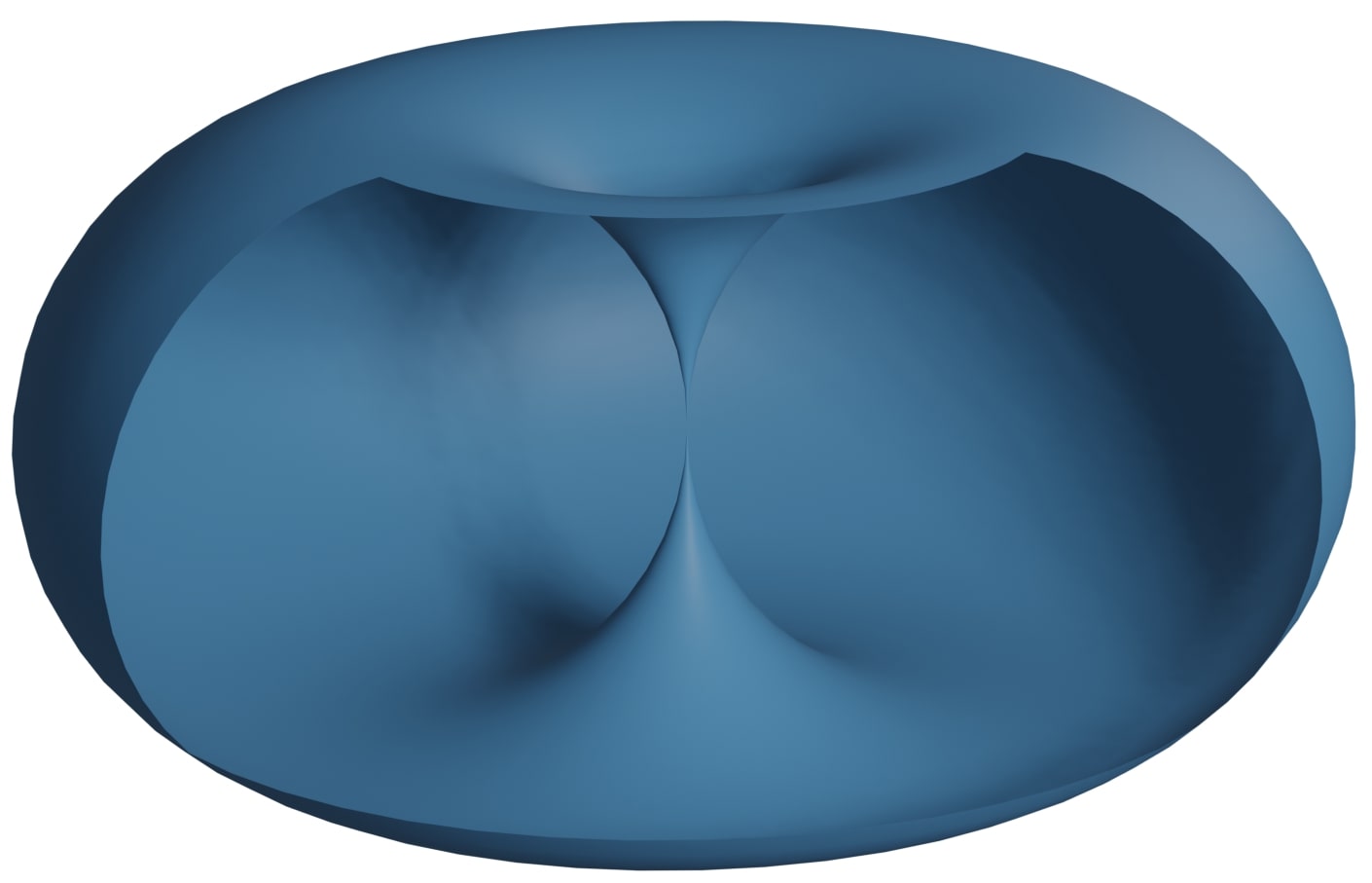
(b) $L=\ell$. Horn torus

(d) Self-intersecting Klein bottle

Figure 5: Representations of the C-space of three double pendulums which, topologically, are tori but whose straightforward inclusions in $\mathbb{R}^{3}$ are not always an embedding. We also depict a self-intersecting inclusion of a Klein bottle in $\mathbb{R}^{3}$.

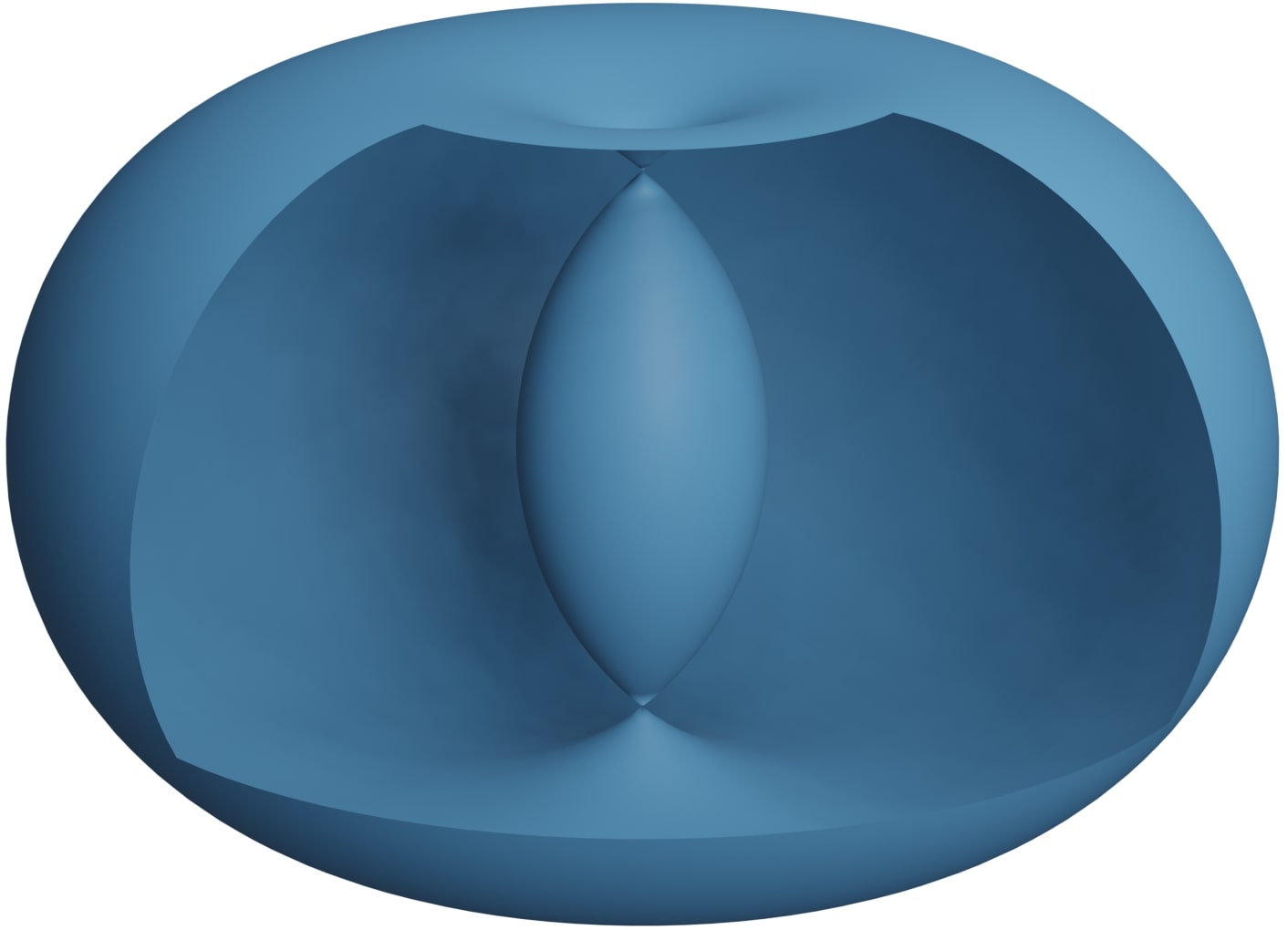
(c) $L<\ell$. Self-intersecting torus

The preceding approach was useful but not easy to generalize. That is why we now consider yet another approach that is better suited for the more general cases that we consider in the rest of the paper. From now, we assume for simplicity that both pendulums move on the same plane, that $L>\ell$, and that the first pendulum is attached to the origin. We will now focus on the endpoint $p$, where we place a pen and try to paint the largest possible circle. To do that, we have to place both pendulums aligned and pointing in the same direction (they are straightened, denoted by , representing both pendulums pointing in the same direction). Then we obtain the circle $\mathbb{S}^{1}_{r^{+}}$ of radius $r^{+}:=L+\ell$. Analogously, the smallest circle around the origin that we can draw is $\mathbb{S}^{1}_{r^{-}}$, obtained when both pendulums are aligned and pointing in opposite directions (they are anti-straightened, denoted by , which represents the first pendulum pointing away from the center and the second pendulum pointing back to the center). We will refer to the circles drawn with these configurations as the max-circle and min-circle, respectively.

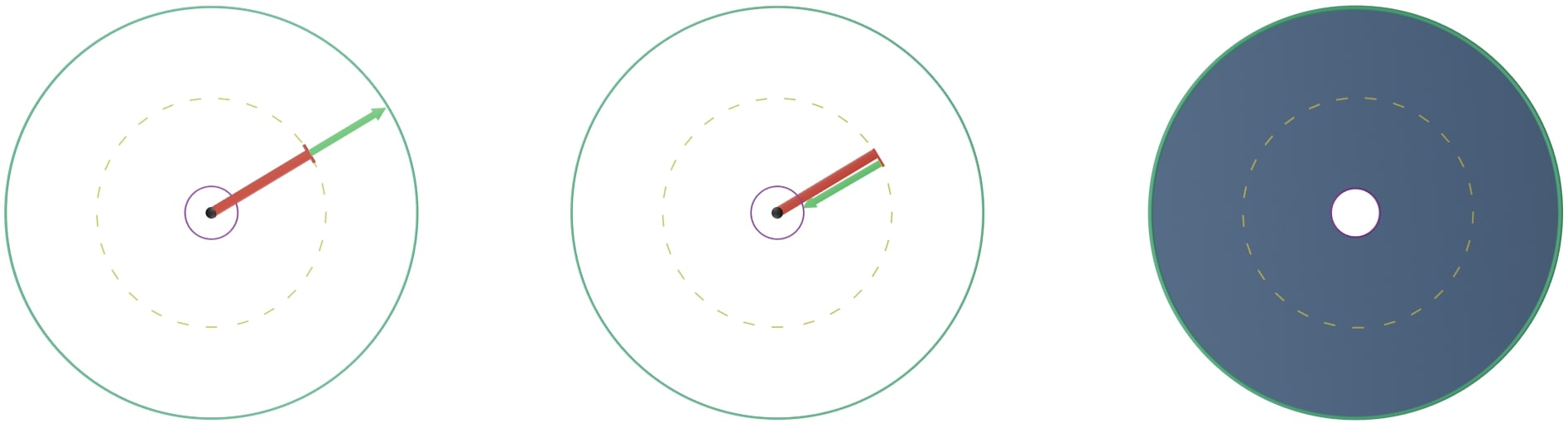
Figure 6: Straight configuration over the max-circle (left). Anti-straight configuration

over the min circle (middle). On the right, we shadow the reachable area, which corresponds with the region in between the max-circle and min-circle. The dashed line on all three images represents the position of the end of the first pendulum, which always describes a circle of radius $L$.

Since the pen at $p$ can also draw over the area in between the circles, we can colour the interior of the annulus as well, which, in polar coordinates, is given by

$$A(L,\ell):=\{(r,\theta)\in\mathbb{R}^{+}\times\mathbb{S}^{1}\ |\ r^{-}<r<r^{+}\}\;.$$

Then, $\mathscr{A}:=\mathbb{S}^{1}_{r^{+}}\cup A(L,\ell)\cup\mathbb{S}^{1}_{r^{-}}$ is the space of all points that $p$ reaches, so we will call it the reachable space (see Fig. 6). This is equivalent to the work space discussed in section 2.3. However, just as for those robot arms, this is not the full C-space (joint space) of the double pendulum. To see that, notice that there are two configurations for every point of $A(L,\ell)$ as shown in Figure 7. Namely, one is when the pendulums are bent in such a way that the angle points in the clockwise direction (that we denote as ) and the symmetric one with respect to the vector $\overline{Op}$ where the angle points in the counterclockwise direction (that we denote as ).

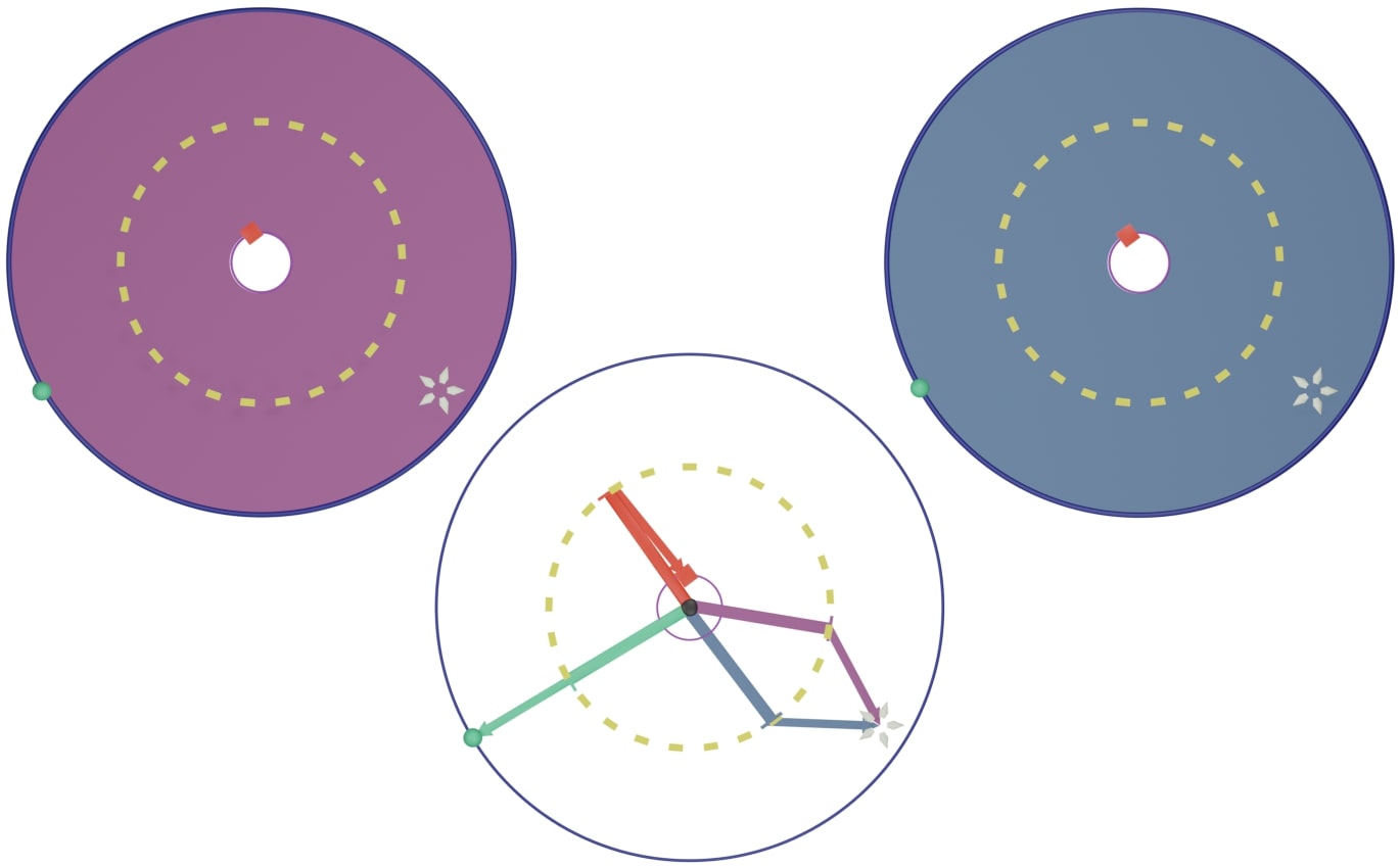
Figure 7: On top, we depict the C-space of the double pendulum: two copies of the annulus corresponding to the (left picture) and (right picture) configurations. Their boundaries are the limit case with the and

configurations. On the bottom, we have the physical world where several configurations are drawn over it: one in purple, one in blue (both with equal endpoints), one in green, and one

in red.

This might lead to thinking that the C-space is two disjoint copies of $\mathscr{A}$, one corresponding to and the other to . However, most readers probably have realized that the previous reasoning does not apply to the boundary circles. Indeed, the points of the max-circle $\mathbb{S}^{1}_{r^{+}}$ only have the configuration while the points of the min-circle $\mathbb{S}^{1}_{r^{-}}$ only have the configuration. In fact, these last two configurations are the limit of both and when we approach the corresponding boundary. The C-space is then obtained, as shown in Figure 8, by taking two copies of $\mathscr{A}$ and identifying (gluing) the interior boundaries together with the same orientation and analogously for the exterior boundaries. In doing so, we obtain something like an inflatable rubber ring or, in the mathematical language, the expected torus!

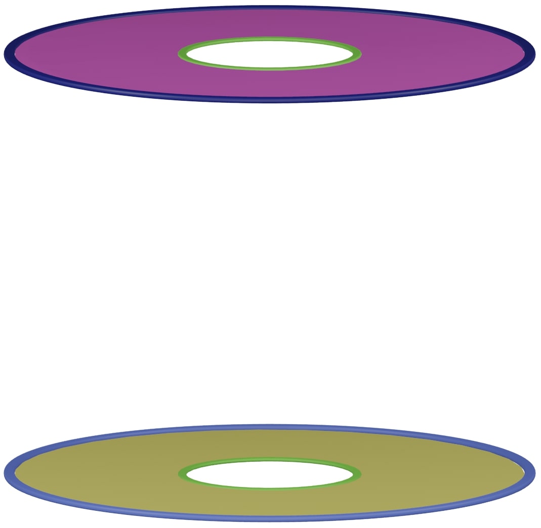
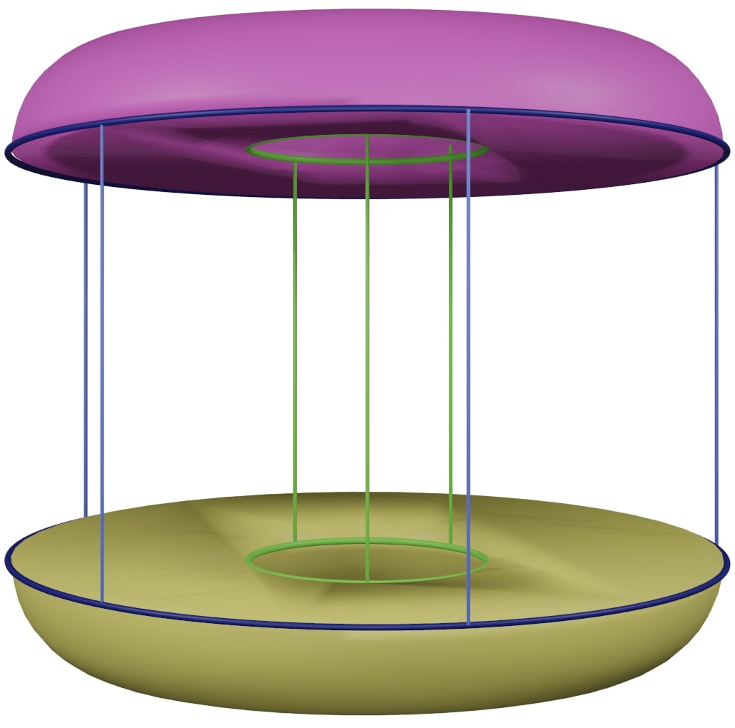
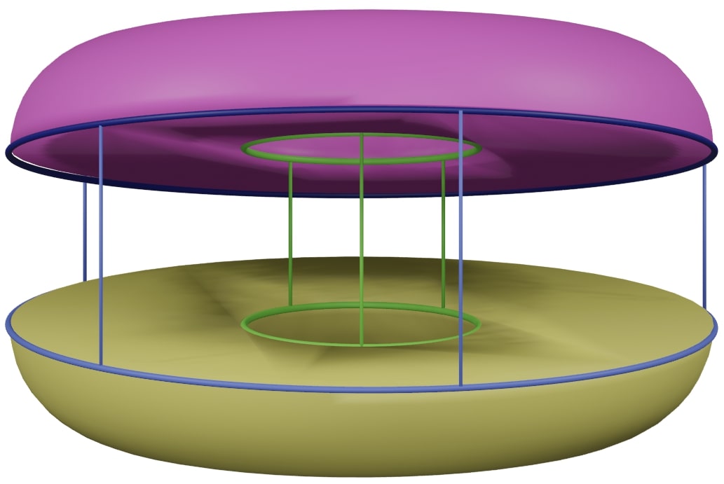
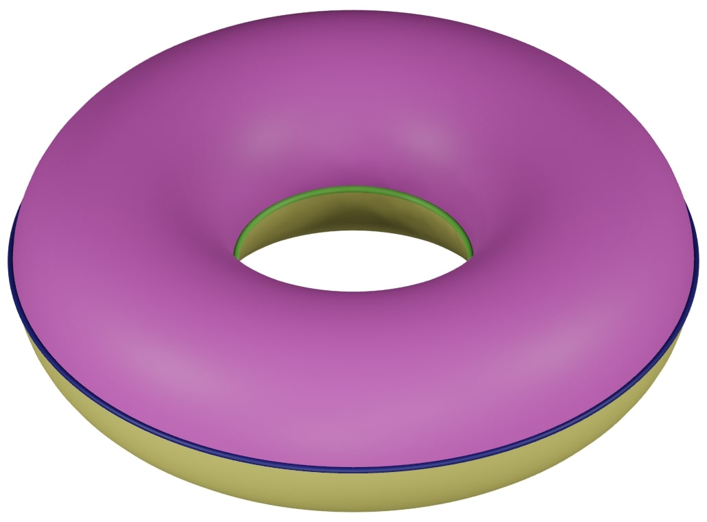
Figure 8: Two annuli with their boundaries identified give rise to a torus.

3.2 Twisted double pendulum

Changing the previous example slightly, we can change the C-space from a torus, which is orientable, to a Klein bottle, which is non-orientable. Recall that a circle $\mathbb{S}^{1}$ can be thought of as a closed interval $[0,2\pi]$ where the endpoints are glued (see Fig. 1). Hence, a torus $\mathbb{S}^{1}\times\mathbb{S}^{1}$ can be thought of as a square $[0,2\pi]\times[0,2\pi]$ where we first glue the vertical sides $\{0\}\times[0,2\pi]$ and $\{2\pi\}\times[0,2\pi]$ with the same orientation to obtain a cylinder. Afterward, we glue the horizontal ones $[0,2\pi]\times\{0\}$ and $[0,2\pi]\times\{2\pi\}$ (the boundaries of the cylinder), again with the same orientation, to obtain the torus. This process is shown in Figure 9.

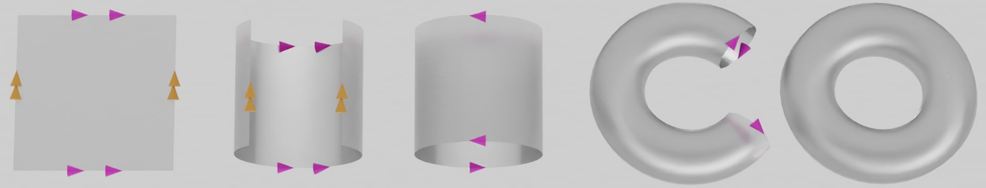
Figure 9: Gluing process to obtain a torus.

If we change the orientation of one of the horizontal sides, when we glue the vertical sides, we obtain a cylinder with boundaries with opposite orientations. Gluing them together leads to a Klein bottle, as shown in Figure 10.

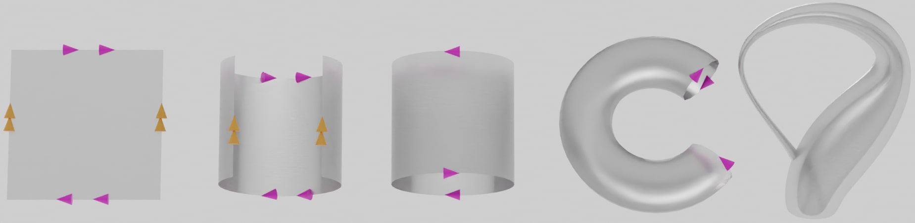
Figure 10: Gluing process to obtain a Klein bottle.

To realize a Klein bottle in a mechanical system, we would have to take a double pendulum and create some sort of gears such that the second pendulum spins along its own axis when the angle of the first pendulum varies (see Figure 11).

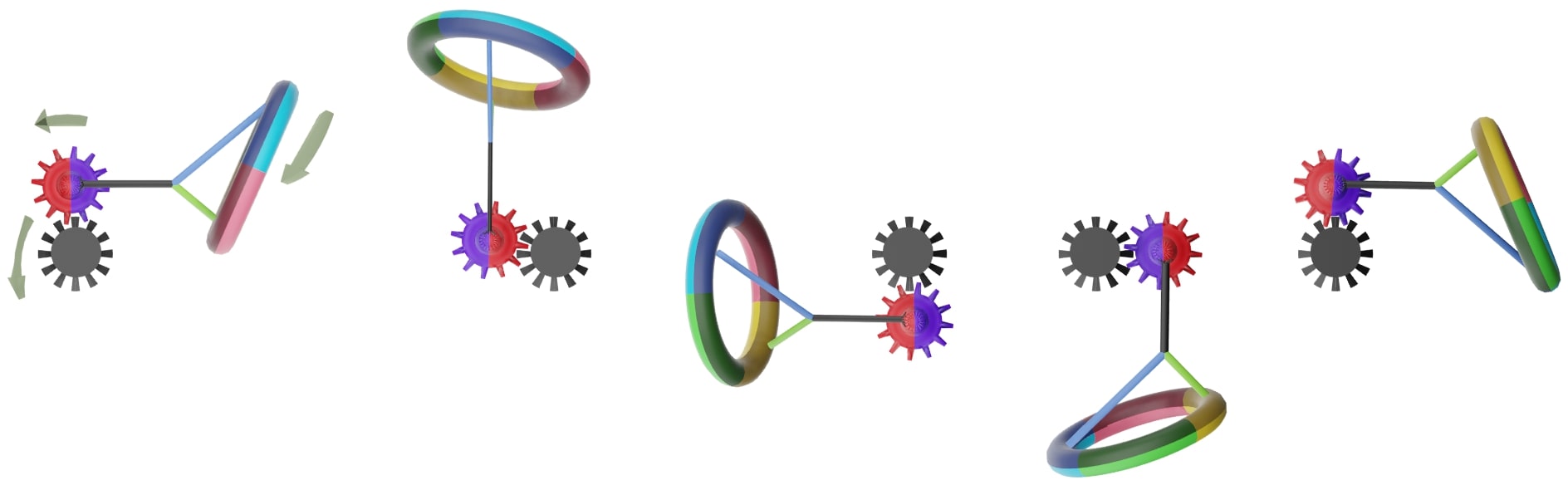
Figure 11: The center gear (in black) is fixed, while the other one (in purple and red) can turn around the fixed one through the gears, which corresponds to the first pendulum. We then attach a rod to the second gear that can turn freely, corresponding to the second pendulum. However, the rod can also spin around its axis (as shown by the coloured circle at the end), but not freely. Such spinning is governed by the position of the first pendulum, as shown in the sequence of images. After a full cycle of the second gear, the circle has turned 180º.

If after one whole turn by the first pendulum (without moving the second one), the second one has twist half-turn along its axis, then the vertical sides $\{0\}\times[0,2\pi]$ and $\{2\pi\}\times[0,2\pi]$ will have different orientation leading to a Klein bottle. This construction was actually described, to the best of our knowledge for the first time, by Richard L.W. Brown [6]. Brown describes this system, which he refers to as the egg-beater, in detail to prove that the C-space is a Klein bottle.

3.3 Simple pendulum over a rail

Suppose that instead of placing the second pendulum at the end of the first pendulum, we place it over a straight rail (equivalently, we can think that we are taking the limit $L\to\infty$). In that case, the C-space is an infinite cylinder $\mathbb{R}\times\mathbb{S}^{1}$ or, if we constrain the movement of the point $m$ of the rail, a finite cylinder. Likewise, if we add some gears so that the orientation of the pendulum changes along the rail, we could get an (infinite) Möbius strip.

3.4 Linkages

Now that we have seen some of the most common examples, let us explore the so-called linkages which will allow us to build more intricate C-spaces. Linkages are links (rigid bars) joined by joints (with ideal rotation) that can be placed at the end of the links or in the middle. The end of the links that are not attached to a joint can be fixed or free. For instance, a double pendulum is a linkage with two links $K_{1},K_{2}$, one joint $J$ joining the end of $K_{1}$ with the beginning of $K_{2}$, one fixed point at the beginning of $K_{1}$, and one free point at the end of $K_{2}$. A pair of scissors is, roughly speaking, formed by two links, one joint placed in the middle of both links, and four free ends. Linkages can be further classified and are essential in engineering, but for our purposes, it is enough to focus on what we call $n$-cranks. We define a crank $C(q,L,\ell)$ as a double pendulum with lengths $L>\ell$ and whose fix point is $q$. We will denote $p$ its free end. A $2$-crank is formed by two cranks $\{C(q_{i},L_{i},\ell_{i})\}_{i=1,2}$ joined by the free end i.e. $p_{1}=p_{2}$. A $3$-crank is given by three cranks where all the free ends $p_{i}$ are merged in a joint. Analogously, we can define the $n$-crank (see Fig. 12). It is easy to check that the number of DOF of an $n$-crank is $2$. Indeed, each crank has a middle point $m_{i}$, adding 2 variables but also two constraints (the distance from the fixed point $q_{i}$ to the middle point $m_{i}$ and the distance from $m_{i}$ to the endpoint $p_{i}$). Hence it does not contribute to the DOFs. The endpoint $p_{i}$ adds two DOFs, and since all $p_{i}$ are identified, two is the total number of DOFs.

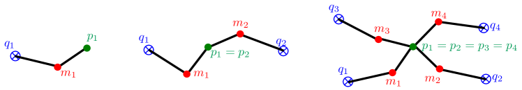
Figure 12: 1-crank, 2-crank, and 4-crank. We have three types of points: the fixed ones ($q_{i}$ in blue), the joint points ($m_{i}$ in red), and the “free” point ($p_{i}$ in green).

3.4.1 2-crank

In order to study the $2$-crank, let us first quickly recall what we did for the double pendulum (the $1$-crank). First, we derived that the reachable space of $p_{1}$ is the space between the max-circle and the min-circle around the fixed point $q_{1}$. We denote from now on that closed region as $\mathscr{A}(q_{1},L_{1},\ell_{1})$, the interior as $A(q_{1},L_{1},\ell_{1})$, and its boundaries as $\mathbb{S}^{1}(q_{1},r_{1}^{\pm})$ where $r_{1}^{\pm}:=L_{1}\pm\ell_{1}$. On the one hand, we have one configuration per boundary point: for the max-circle and for the min-circle. On the other hand, we have two configurations per interior point: and . This leads to a C-space formed by two copies of the annulus where the boundaries are identified, i.e., the expected torus.

For the $2$-crank, we have to repeat the process twice and look for the intersection. Indeed, $p_{i}$ can reach every point in $\mathscr{A}(q_{i},L_{i},\ell_{i})$ but since $p_{1}=p_{2}$, the reachable space of the $2$-crank is

$$\mathscr{R}_{2}:=\mathscr{A}\!\left(q_{1},L_{1},\ell_{1}\right)\cap\mathscr{A}\!\left(q_{2},L_{2},\ell_{2}\right)$$

which can take different shapes depending on the parameters involved $(q_{i},L_{i},\ell_{i})$. In particular, it could be empty if $q_{1}$ is too far apart from $q_{2}$. It could be just a point if the distance between the centers is precisely $L_{1}+\ell_{1}+L_{2}+\ell_{2}$. Or it could have several connected components (see Fig. 13).

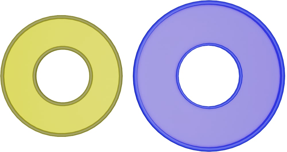
(a) Too far apart. Empty intersection.

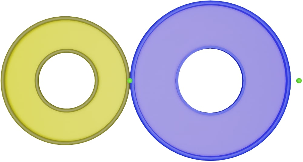
(b) Only one possible configuration.

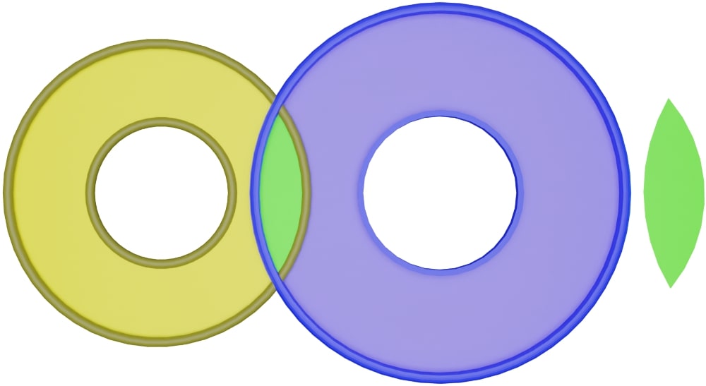
(c) “Oval” or “$2$-agon”.

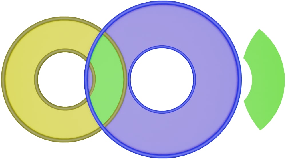
(d) “4-agon”.

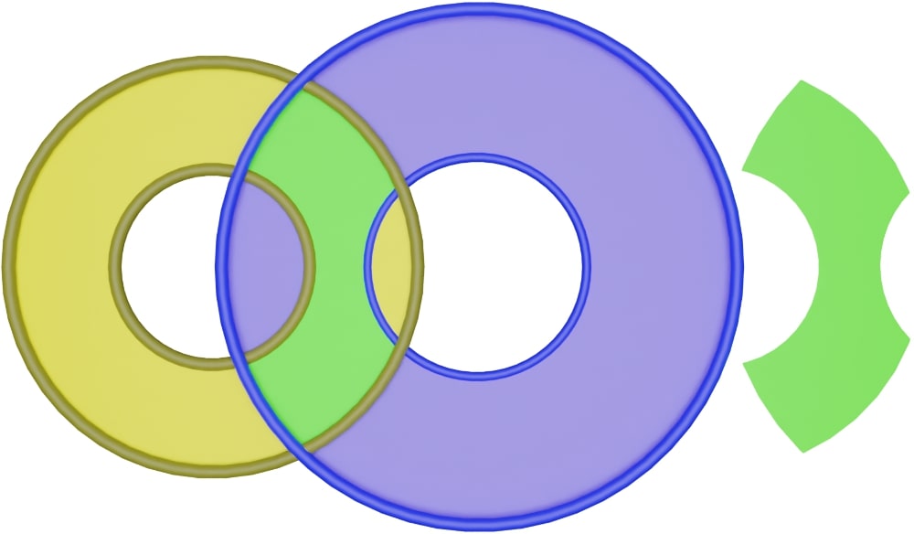
(e) “$6$-agon”.

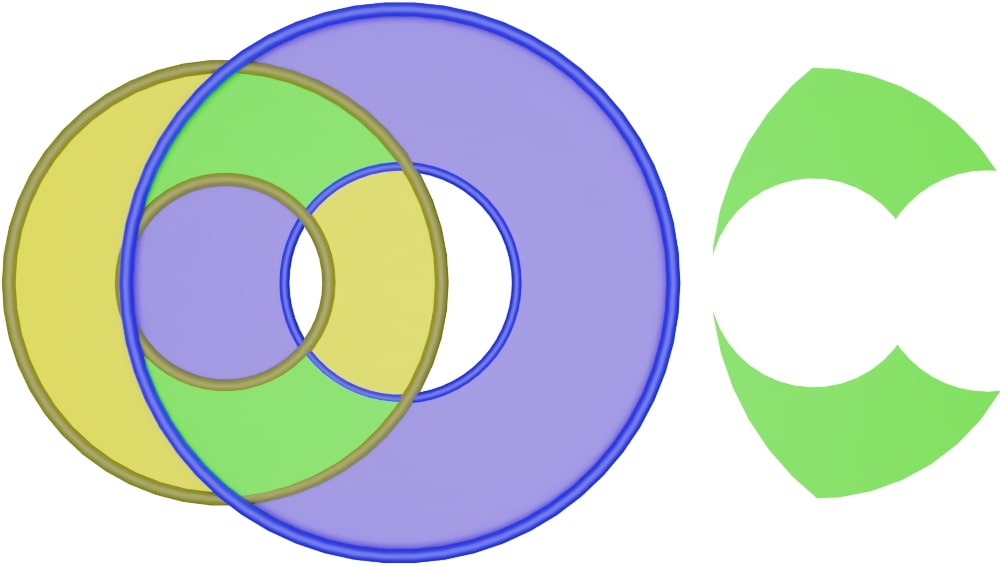
(f) More intricate reachable space.

Figure 13: The left annulus (yellow) represents the reachable space of the first pendulum, while the right annulus (blue) represents the reachable space of the second pendulum. The intersection is highlighted on the side of each image (green). Notice that in this simple case, we can exhaust every possible reachable area by moving the right annulus slowly to the left, starting from Figure 13(a) and ending in the symmetric configuration, where the yellow and blue annuli are swapped.

Now we proceed to study the possible configurations for each point of $\mathscr{R}_{2}$. In the interior, each crank can be in the or configuration, while, at the boundary, the $i$-th crank has only one possible configuration ( for the max-circle and for the min-circle, see Fig. 7). We see that we have $4\times 4=16$ possible configurations summarized in the following table:

Possible configurations	Region	Further explanation
$($1st crank, 2nd crank$)$
$(\!\!\raisebox{0.96873pt}{ \leavevmode\hbox to7.51pt{\vbox to4.53pt{\text{[drawing]}}}},\!\!\raisebox{0.96873pt}{ \leavevmode\hbox to7.51pt{\vbox to4.53pt{\text{[drawing]}}}})$	$A\!\left(q_{1},L_{1},\ell_{1}\right)\cap A\!\left(q_{2},L_{2},\ell_{2}\right)$
$(\!\!\raisebox{0.96873pt}{ \leavevmode\hbox to7.51pt{\vbox to4.53pt{\text{[drawing]}}}},\!\!\raisebox{0.38751pt}{ \leavevmode\hbox to7.51pt{\vbox to5.18pt{\text{[drawing]}}}})$		Both cranks in the interior of their
$(\!\!\raisebox{0.38751pt}{ \leavevmode\hbox to7.51pt{\vbox to5.18pt{\text{[drawing]}}}},\!\!\raisebox{0.96873pt}{ \leavevmode\hbox to7.51pt{\vbox to4.53pt{\text{[drawing]}}}})$		respective annulus (2 conf. each).
$(\!\!\raisebox{0.38751pt}{ \leavevmode\hbox to7.51pt{\vbox to5.18pt{\text{[drawing]}}}},\!\!\raisebox{0.38751pt}{ \leavevmode\hbox to7.51pt{\vbox to5.18pt{\text{[drawing]}}}})$
$(\!\!\raisebox{0.96873pt}{ \leavevmode\hbox to7.51pt{\vbox to4.53pt{\text{[drawing]}}}},\!\!\raisebox{-0.96873pt}{ \leavevmode\hbox to4.67pt{\vbox to7.51pt{\text{[drawing]}}}})$	$A\!\left(q_{1},L_{1},\ell_{1}\right)\cap\mathbb{S}^{1}(q_{2},r_{2}^{+})$	1st crank in the interior (2 conf.),
$(\!\!\raisebox{0.38751pt}{ \leavevmode\hbox to7.51pt{\vbox to5.18pt{\text{[drawing]}}}},\!\!\raisebox{-0.96873pt}{ \leavevmode\hbox to4.67pt{\vbox to7.51pt{\text{[drawing]}}}})$		2nd one over max-circle (1 conf.).
$(\!\!\raisebox{0.96873pt}{ \leavevmode\hbox to7.51pt{\vbox to4.53pt{\text{[drawing]}}}},\!\!\scalebox{1.2}{\raisebox{-0.96873pt}{ \leavevmode\hbox to5.21pt{\vbox to6.08pt{\text{[drawing]}}}}})$	$A\!\left(q_{1},L_{1},\ell_{1}\right)\cap\mathbb{S}^{1}(q_{2},r_{2}^{-})$	1st crank in the interior (2 conf.),
$(\!\!\raisebox{0.38751pt}{ \leavevmode\hbox to7.51pt{\vbox to5.18pt{\text{[drawing]}}}},\!\!\scalebox{1.2}{\raisebox{-0.96873pt}{ \leavevmode\hbox to5.21pt{\vbox to6.08pt{\text{[drawing]}}}}})$		2nd one over min-circle (1 conf.).
$(\!\!\raisebox{-0.96873pt}{ \leavevmode\hbox to4.67pt{\vbox to7.51pt{\text{[drawing]}}}},\!\!\raisebox{0.96873pt}{ \leavevmode\hbox to7.51pt{\vbox to4.53pt{\text{[drawing]}}}})$	$\mathbb{S}^{1}(q_{1},r_{1}^{+})\cap A\!\left(q_{2},L_{2},\ell_{2}\right)$	1st crank over max-circle (1 conf.),
$(\!\!\raisebox{-0.96873pt}{ \leavevmode\hbox to4.67pt{\vbox to7.51pt{\text{[drawing]}}}},\!\!\raisebox{0.38751pt}{ \leavevmode\hbox to7.51pt{\vbox to5.18pt{\text{[drawing]}}}})$		2nd one in the interior (2 conf.).
$(\!\!\scalebox{1.2}{\raisebox{-0.96873pt}{ \leavevmode\hbox to5.21pt{\vbox to6.08pt{\text{[drawing]}}}}},\!\!\raisebox{0.96873pt}{ \leavevmode\hbox to7.51pt{\vbox to4.53pt{\text{[drawing]}}}})$	$\mathbb{S}^{1}(q_{1},r_{1}^{-})A\cap\!\left(q_{2},L_{2},\ell_{2}\right)$	1st crank over min-circle (1 conf.),
$(\!\!\scalebox{1.2}{\raisebox{-0.96873pt}{ \leavevmode\hbox to5.21pt{\vbox to6.08pt{\text{[drawing]}}}}},\!\!\raisebox{0.38751pt}{ \leavevmode\hbox to7.51pt{\vbox to5.18pt{\text{[drawing]}}}})$		2nd one in the interior (2 conf.).
$(\!\!\raisebox{-0.96873pt}{ \leavevmode\hbox to4.67pt{\vbox to7.51pt{\text{[drawing]}}}},\!\!\raisebox{-0.96873pt}{ \leavevmode\hbox to4.67pt{\vbox to7.51pt{\text{[drawing]}}}})$	$\mathbb{S}^{1}(q_{1},r_{1}^{+})\cap\mathbb{S}^{1}(q_{2},r_{2}^{+})$	Both max-circles (1 conf. each).
$(\!\!\raisebox{-0.96873pt}{ \leavevmode\hbox to4.67pt{\vbox to7.51pt{\text{[drawing]}}}},\!\!\scalebox{1.2}{\raisebox{-0.96873pt}{ \leavevmode\hbox to5.21pt{\vbox to6.08pt{\text{[drawing]}}}}})$	$\mathbb{S}^{1}(q_{1},r_{1}^{+})\cap\mathbb{S}^{1}(q_{2},r_{2}^{-})$	Max-circle and min-circle (1 conf. each).
$(\!\!\scalebox{1.2}{\raisebox{-0.96873pt}{ \leavevmode\hbox to5.21pt{\vbox to6.08pt{\text{[drawing]}}}}},\!\!\raisebox{-0.96873pt}{ \leavevmode\hbox to4.67pt{\vbox to7.51pt{\text{[drawing]}}}})$	$\mathbb{S}^{1}(q_{1},r_{1}^{-})\cap\mathbb{S}^{1}(q_{2},r_{2}^{+})$	Min-circle and max-circle (1 conf. each).
$(\!\!\scalebox{1.2}{\raisebox{-0.96873pt}{ \leavevmode\hbox to5.21pt{\vbox to6.08pt{\text{[drawing]}}}}},\!\!\scalebox{1.2}{\raisebox{-0.96873pt}{ \leavevmode\hbox to5.21pt{\vbox to6.08pt{\text{[drawing]}}}}})$	$\mathbb{S}^{1}(q_{1},r_{1}^{-})\cap\mathbb{S}^{1}(q_{2},r_{2}^{-})$	Both min-circles (1 conf. each).

Notice that some of the regions of this table can be empty or reduced just to a point. Let us explore a couple of examples and determine the C-space.

2-crank - Gluing for the 2-agon case
We have already mentioned that if $\mathrm{d}(q_{1},q_{2})=r^{+}_{1}+r^{+}_{2}$ then the only possible configuration is $(\!\!\raisebox{-0.96873pt}{ \leavevmode\hbox to4.67pt{\vbox to7.51pt{\text{[drawing]}}}},\!\!\raisebox{-0.96873pt}{ \leavevmode\hbox to4.67pt{\vbox to7.51pt{\text{[drawing]}}}})$ and the C-space is only one point. The next case to consider is when the distance is slightly smaller:

$$\mathrm{max}\{r^{+}_{1}+r^{-}_{2},r^{-}_{1}+r^{+}_{1}\}<\mathrm{d}(q_{1},q_{2})<r^{+}_{1}+r^{+}_{2}\;.$$ (8)

Then the reachable space is an oval ($2$-agon) as depicted in Figure 13(c). The second inequality ensures that both cranks can be bent, while the first one ensures that none of the min-circles are reachable, i.e., the configuration is not available to either of the cranks. Removing such configurations from the table leaves us with a C-space formed by four ovals whose edges have at least one configuration as the following image suggests

To simplify the resulting C-space, we proceed as we did for Figure 7. First, we glue the edges $(\!\!\raisebox{0.96873pt}{ \leavevmode\hbox to7.51pt{\vbox to4.53pt{\text{[drawing]}}}},\!\!\raisebox{-0.96873pt}{ \leavevmode\hbox to4.67pt{\vbox to7.51pt{\text{[drawing]}}}})$ of the first two ovals and the edges $(\!\!\raisebox{0.38751pt}{ \leavevmode\hbox to7.51pt{\vbox to5.18pt{\text{[drawing]}}}},\!\!\raisebox{-0.96873pt}{ \leavevmode\hbox to4.67pt{\vbox to7.51pt{\text{[drawing]}}}})$ of the last two ovals, leading to the following two disks

with equivalent boundaries. If we glue them, we obtain that the C-space is a sphere.

2-crank - Gluing for the 4-agon case
The next case to consider is when the centers are separated such that the boundary of the reachable region is formed by one of the min-circles and by both of the max-circles (see Fig. 13(d)):

$$r^{-}_{1}<\mathrm{d}(q_{1},q_{2})-r^{+}_{2}<\mathrm{d}(q_{1},q_{2})-r^{-}_{2}<r^{+}_{1}<\mathrm{d}(q_{1},q_{2})$$ (9)

Then, we end up with four $2$-agons (they can also be obtained by removing a piece of a disk from each of the ovals of the previous case)

We now glue the edges $(\!\!\raisebox{0.96873pt}{ \leavevmode\hbox to7.51pt{\vbox to4.53pt{\text{[drawing]}}}},\!\!\raisebox{-0.96873pt}{ \leavevmode\hbox to4.67pt{\vbox to7.51pt{\text{[drawing]}}}})$ of the first two $4$-agons and the edges $(\!\!\raisebox{0.38751pt}{ \leavevmode\hbox to7.51pt{\vbox to5.18pt{\text{[drawing]}}}},\!\!\raisebox{-0.96873pt}{ \leavevmode\hbox to4.67pt{\vbox to7.51pt{\text{[drawing]}}}})$ of the last two $4$-agons, leading to two annuli

    

with the boundaries identified. Thus the C-space is a torus.

The avid reader might have realized that the C-space has changed its topology from a sphere to a torus by continuously decreasing $\mathrm{d}(q_{1},q_{2})$. This change can be understood as a phase transition where the inner hole of the torus collapses to a point when the cranks get closer or, conversely, where we create a puncture on the sphere when the cranks get further apart.

2-crank - Gluing for the 6-agon case
We leave as an exercise to the reader to prove, using the same techniques, that the C-space when

$$0<\mathrm{d}(q_{1},q_{2})-r^{+}_{2}<r^{-}_{1}<\mathrm{d}(q_{1},q_{2})-r^{-}_{2}<r^{+}_{1}<\mathrm{d}(q_{1},q_{2})$$

is given by this C-space

and that, upon gluing the equivalent boundaries, leads to a topological surface with two holes.

2-crank - Euler characteristic
Although this gluing strategy to determine the C-space is very visual and easy to implement in these examples, it becomes harder when more cranks are involved. That is why we present an alternative derivation that relies on the fact that the topology of compact surfaces is completely characterized by two parameters: the orientability and the genus of the surface. The proof of this fact can be found in any book of algebraic topology or surface topology like [7, Ch.12]. The genus, in turn, is characterized by the Euler characteristic $\textstyle\chi$, which can be computed following these steps

1. Take any triangulation of the surface.

2. Count the number of triangles (faces) $F$, the number of edges $E$, and the number of vertices $V$.

3. Compute its alternate sum

   $${\mathchoice{\raisebox{0.0pt}{$\displaystyle\chi$}}{\raisebox{0.0pt}{$\textstyle\chi$}}{\raisebox{0.0pt}{$\scriptstyle\chi$}}{\raisebox{0.0pt}{$\scriptscriptstyle\chi$}}}=F-E+V$$

It can be proved that this number does not depend on the triangulation (for instance, if we break a triangle into two, we increase $F$ by one, $E$ by 2, and $V$ by 1, so $\textstyle\chi$ does not change). Moreover, it can be proved that

$${\mathchoice{\raisebox{0.0pt}{$\displaystyle\chi$}}{\raisebox{0.0pt}{$\textstyle\chi$}}{\raisebox{0.0pt}{$\scriptstyle\chi$}}{\raisebox{0.0pt}{$\scriptscriptstyle\chi$}}}=\begin{cases}2(1-g)&\text{If the surface is orientable}\\ 2-g&\text{If the surface is non-orientable}\end{cases}$$

where $g$ is the genus of the surface. For orientable surfaces, the genus is the number of holes: zero for the sphere, 1 for the torus, and so on. For non-orientable surfaces, it is a bit more complicated. Luckily, all the surfaces considered from now on turn out to be orientable.

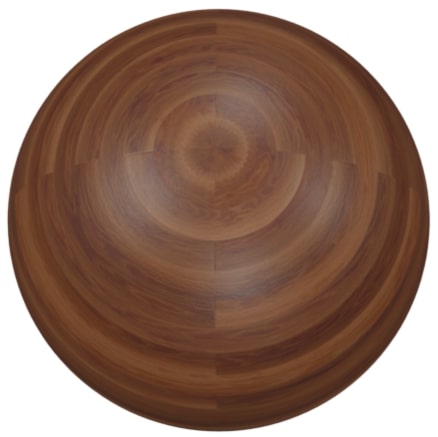
(a) g = 0

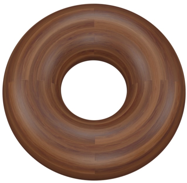
(b) g = 1

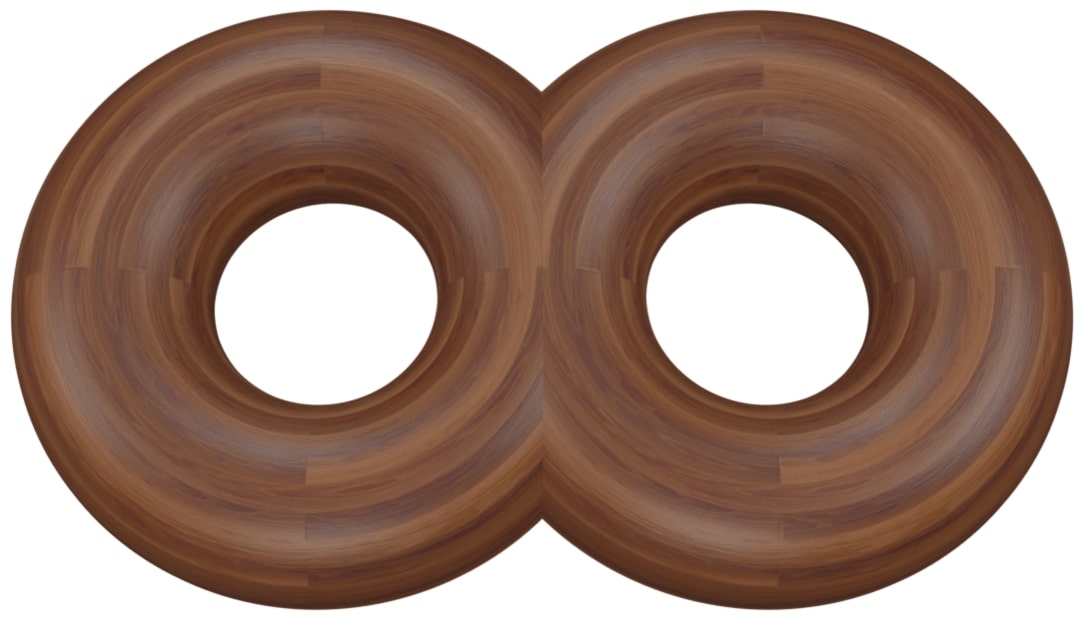
(c) g = 2

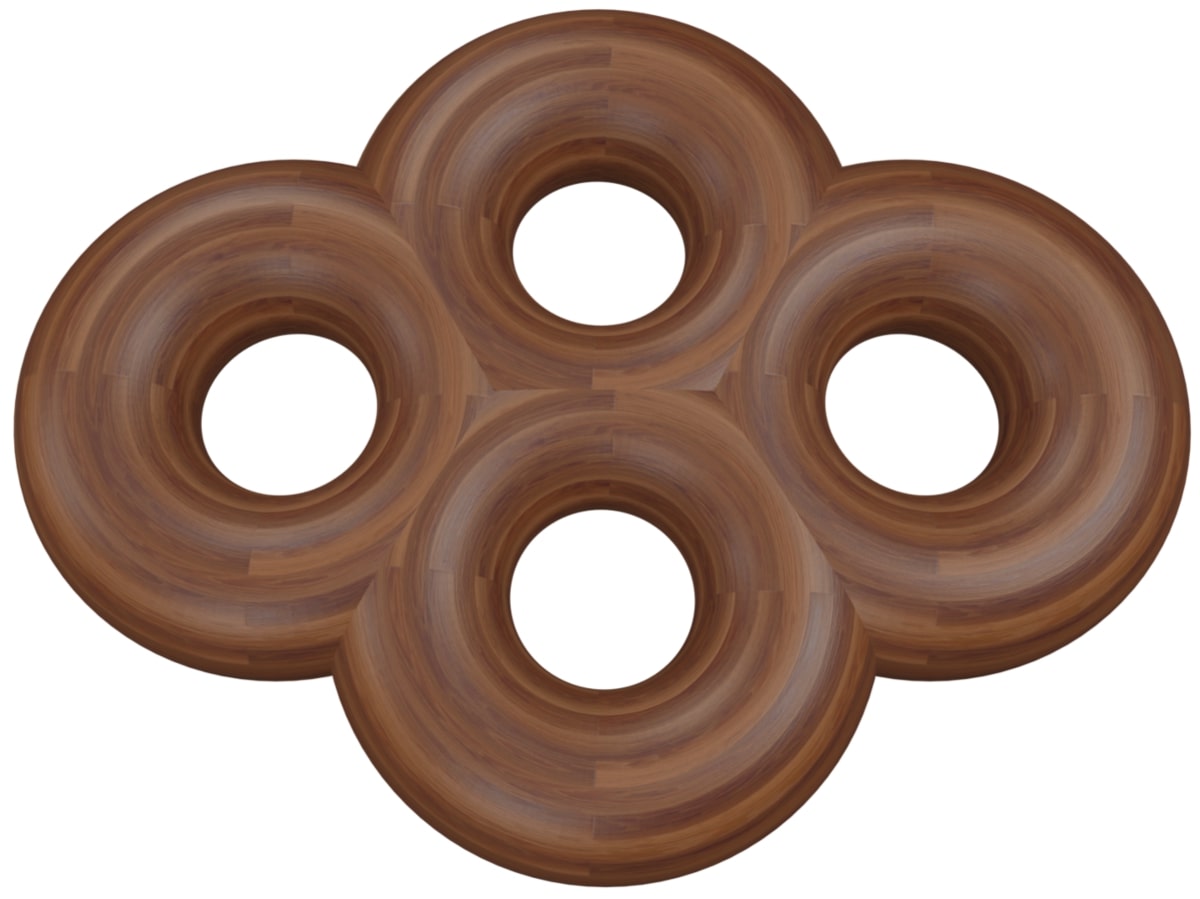
(d) g = 4

Figure 14: Several topological orientable manifolds with different genera.

The last fact that we need is that we can generalize the construction of the torus and Klein bottle that we mentioned in section 3.2 where we identified sides. Recall that for the former, we considered a square where the opposite sides were identified with the same orientation (see Fig. 9), while for the latter, two of the identified sides had opposite orientation (see Fig. 10). The best way to write this is with the alphabet representation: pick a point, follow the graph clockwise and assign letters $a,b,c\ldots$ to the edges whenever we are following the arrow of the edge and their inverse $a^{-1},b^{-1},c^{-1}\ldots$ whenever we go against the arrow. The identified edges will have the same letter (up to orientation). The alphabet representation of the torus is $aba^{-1}b^{-1}$ while the one for the Klein bottle is $abab^{-1}$.

It is worth noting that, as the notation suggests, $\cdots acc^{-1}b\cdots=\cdots ab\cdots$ since identifying these edges is equivalent to removing them

Finally, notice that in the alphabet representation of the torus, which is orientable, for every letter, we have its opposite. Meanwhile, for the Klein bottle, which is non-orientable, we have two $a$ and no $a^{-1}$. This is actually the defining property of orientable surfaces [7]:

A surface is orientable if and only if for every letter of its alphabet representation, it contains its inverse.

Now let us apply what we have learned to the previous examples. In the $2$-agon case of the 2-crank above, we have $F=1\times 4$ (one for each oval), $E=2\times 4/2=4$ (there are two sides for each of the 4 ovals, but half of them are the same since they are identified), and $V=2\times 4/4=2$ (the top vertex of every oval is identified and the same for the bottom one), which gives an Euler characteristic of ${\mathchoice{\raisebox{0.0pt}{$\displaystyle\chi$}}{\raisebox{0.0pt}{$\textstyle\chi$}}{\raisebox{0.0pt}{$\scriptstyle\chi$}}{\raisebox{0.0pt}{$\scriptscriptstyle\chi$}}}=2$ so the genus is $g=0$ and this implies that the surface is orientable (non-orientable surfaces have $g>0$) and hence the surface is a sphere. Notice that to compute the Euler characteristic, we did not use a triangulation since the faces have four sides. In this case, the result does not change, but, in other cases, the result might vary, so it is always safer to break the faces into triangles.

For the $4$-agon case, a similar count leads to $(F,E,V)=(4,8,4)$, so ${\mathchoice{\raisebox{0.0pt}{$\displaystyle\chi$}}{\raisebox{0.0pt}{$\textstyle\chi$}}{\raisebox{0.0pt}{$\scriptstyle\chi$}}{\raisebox{0.0pt}{$\scriptscriptstyle\chi$}}}=0$. It can be proved that surfaces obtained through this gluing process for $n$-cranks are orientable. Hence, $g=1$, and the surface is a torus. Finally, the $6$-agon case we left as an exercise for the reader can be quickly solved. A quick count leads to $(F,E,V)=(4,12,6)$. Thus ${\mathchoice{\raisebox{0.0pt}{$\displaystyle\chi$}}{\raisebox{0.0pt}{$\textstyle\chi$}}{\raisebox{0.0pt}{$\scriptstyle\chi$}}{\raisebox{0.0pt}{$\scriptscriptstyle\chi$}}}=-2$, which implies $g=2$.

2-crank - General case
After studying these examples, we can deduce a few general properties. Firstly, we can study each connected component separately (see, for instance Fig. 13(e)), since they will define disconnected topological manifolds. Thus, the number of faces $F$ is always $1$ times the number of distinct configurations in the interior of the reachable space. As we have two possible configurations for each crank, hence $F=2^{2}$. Secondly, the number of edges of the reachable space, that we denote $k$, is variable, but over each edge, one of the cranks is locked in the or configuration, while the other crank has two configurations. Hence $E=2^{2-1}k$. Finally, the number of vertices of the reachable area is the same as the number of edges (it is a loop), but their two cranks are fixed into the or configuration, hence $V=2^{2-2}k$. With that information, we obtain that the C-space is an orientable surface of genus

$$g=\frac{k}{2}-1$$

for some $k$ to be determined in each example. As one expects, $k$ is always even in the “nice” examples. However, this formula does not cover the degenerate cases that happen when we have one of the equalities in (8) or (9). Those examples correspond to the in-between cases during the “phase transition” mentioned earlier (when the topology changes). We will see an example in the next section.

3.4.2 3-crank

Let us focus our attention now on the $3$-crank. One particular configuration of this system was studied in depth by Thurston and Weeks in [8] and was a big inspiration to write this paper. We highly recommend it to the interested reader.

The reachable space of the 3-crank is

$$\mathscr{R}_{3}:=\mathscr{A}\!\left(q_{1},L_{1},\ell_{1}\right)\cap\mathscr{A}\!\left(q_{2},L_{2},\ell_{2}\right)\cap\mathscr{A}\!\left(q_{3},L_{3},\ell_{3}\right)$$

Some of the possible regions are shown in Figure 15.

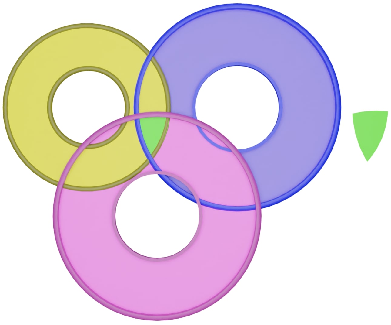
(a) $3$-agon, only max-circles involved. 

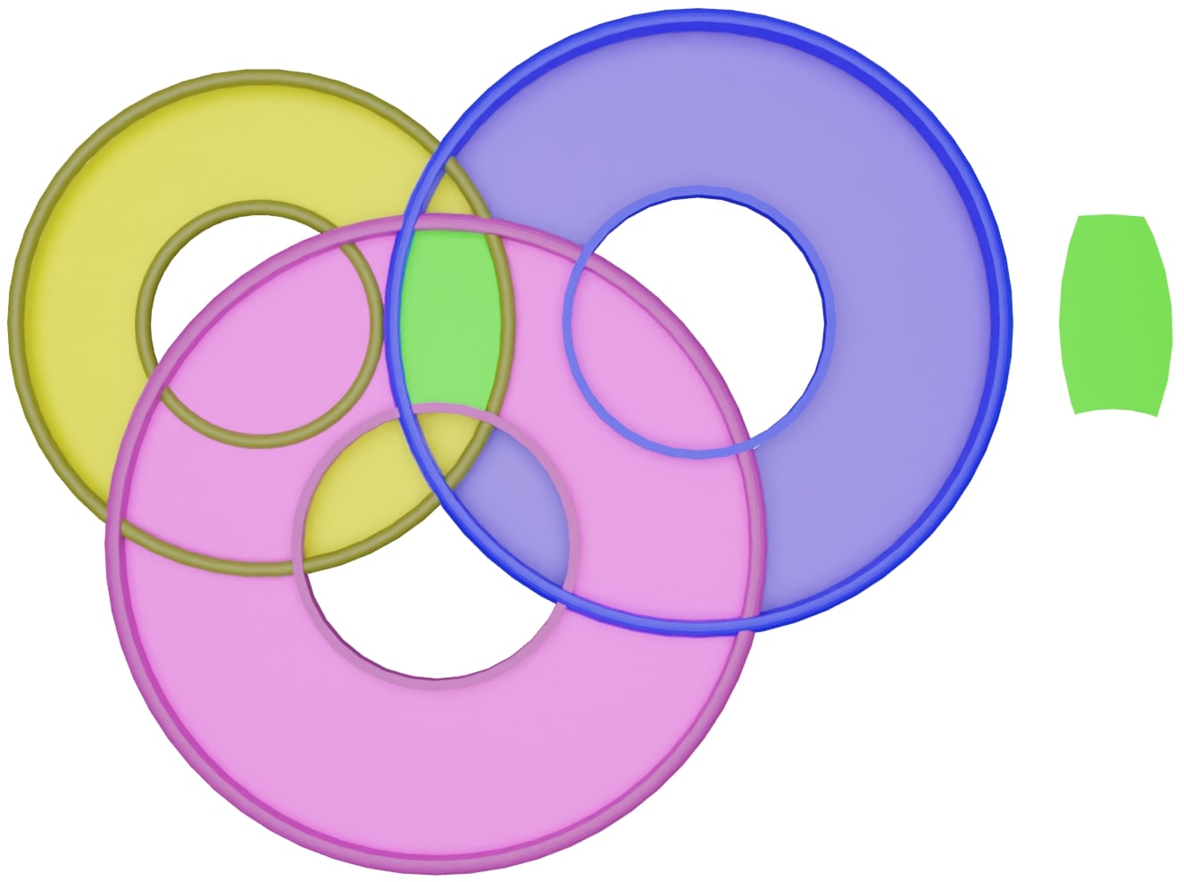
(b) $4$-agon, only one min-circle involved.

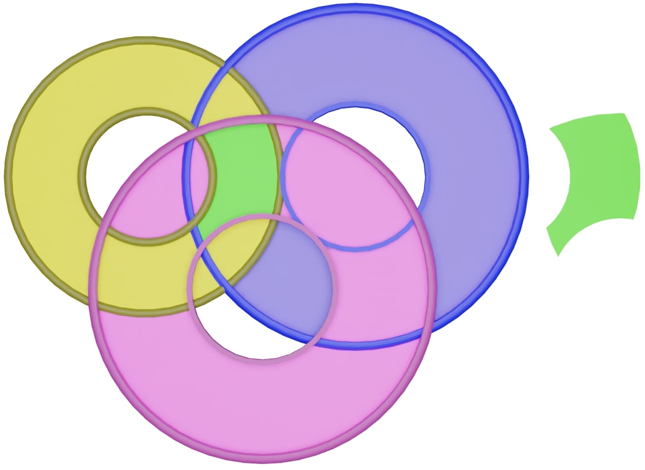
(c) $6$-agon, every min-circle and max-circle involved.

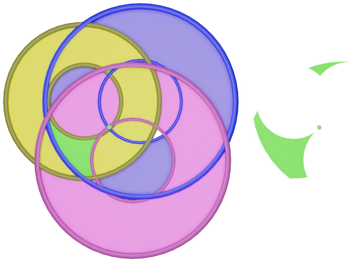
(d) A more intricated reachable area.

Figure 15: The top-left annulus (yellow) of each image represents the reachable region of the first pendulum. The top-right annulus (blue), the reachable space of the second pendulum. The bottom one (pink), the reachable region of the third pendulum. The intersection is highlighted on the side of each image (green).

Although we are not going to build a detailed table of all possible configurations like before, since it would be far too lengthy for this discussion, notice that the $4\times 4\times 4=64$ possible configurations are

$$\{(x_{1},x_{2},x_{3})\text{ where }x_{i}\in\{\!\!\raisebox{0.96873pt}{ \leavevmode\hbox to7.51pt{\vbox to4.53pt{\text{[drawing]}}}},\!\!\raisebox{0.38751pt}{ \leavevmode\hbox to7.51pt{\vbox to5.18pt{\text{[drawing]}}}},\!\!\raisebox{-0.96873pt}{ \leavevmode\hbox to4.67pt{\vbox to7.51pt{\text{[drawing]}}}},\!\!\scalebox{1.2}{\raisebox{-0.96873pt}{ \leavevmode\hbox to5.21pt{\vbox to6.08pt{\text{[drawing]}}}}}\}\}$$

Let us compute the C-space of a couple of examples.

3-crank - Euler characteristic for the 3-agon case
The first example is the $3$-agon depicted in Figure 15(a). The number of faces is $1$ times the number of possible configurations (2 per crank). The number of edges is $3$ times the number of possible configurations (2 per each of the two free cranks, while the other is locked). The number of vertices is $3$ times the number of possible configurations (2 for the free crank, while the other two are locked). Thus

$$\begin{array}[]{l}F=1\times 2^{3}=8\\ E=3\times 2^{3-1}=12\\ V=3\times 2^{3-2}=6\end{array}\qquad\longrightarrow\qquad{\mathchoice{\raisebox{0.0pt}{$\displaystyle\chi$}}{\raisebox{0.0pt}{$\textstyle\chi$}}{\raisebox{0.0pt}{$\scriptstyle\chi$}}{\raisebox{0.0pt}{$\scriptscriptstyle\chi$}}}=2\qquad\longrightarrow\qquad g=1-\frac{\chi}{2}=0$$

and we obtain a sphere.

3-crank - Euler characteristic for the 6-agon case
Let us consider now the case provided in Figure 15(c). Using the same reasoning, we get

$$\begin{array}[]{l}F=1\times 2^{3}=8\\ E=6\times 2^{3-1}=24\\ V=6\times 2^{3-2}=12\end{array}\qquad\longrightarrow\qquad{\mathchoice{\raisebox{0.0pt}{$\displaystyle\chi$}}{\raisebox{0.0pt}{$\textstyle\chi$}}{\raisebox{0.0pt}{$\scriptstyle\chi$}}{\raisebox{0.0pt}{$\scriptscriptstyle\chi$}}}=-4\qquad\longrightarrow\qquad g=1-\frac{\chi}{2}=3$$

which is a torus with three holes.

3-crank - Euler characteristic for the general (nondegenerate) case
As for the $2$-crank case, we have a formula that covers several cases. Indeed, each connected component is given by a $k$-agon with

$$\begin{array}[]{l}F=1\times 2^{3}=8\\ E=k\times 2^{3-1}=4k\\ V=k\times 2^{3-2}=2k\end{array}\qquad\longrightarrow\qquad{\mathchoice{\raisebox{0.0pt}{$\displaystyle\chi$}}{\raisebox{0.0pt}{$\textstyle\chi$}}{\raisebox{0.0pt}{$\scriptstyle\chi$}}{\raisebox{0.0pt}{$\scriptscriptstyle\chi$}}}=8-2k\qquad\longrightarrow\qquad g=1-\frac{\chi}{2}=k-3$$

3-crank - A degenerate case
As we mentioned for the $2$-crank, the previous formula does not cover the degenerate cases, which have to be dealt with separately. Consider, for instance, the following configuration

It might seem that we are in the $3$-agon case previously studied, and the C-space is again a sphere. However, the bottom vertex (blue circle) is different from the top ones (orange squares). Indeed, the former is the intersection of three circles meaning that all three cranks are locked, and the only possible configuration is $(\!\!\raisebox{-0.96873pt}{ \leavevmode\hbox to4.67pt{\vbox to7.51pt{\text{[drawing]}}}},\!\!\raisebox{-0.96873pt}{ \leavevmode\hbox to4.67pt{\vbox to7.51pt{\text{[drawing]}}}},\!\!\scalebox{1.2}{\raisebox{-0.96873pt}{ \leavevmode\hbox to5.21pt{\vbox to6.08pt{\text{[drawing]}}}}})$. The other two vertices have the last crank free, so there are two configurations each. Thus, the counting is now

$$\begin{array}[]{l}F=1\times 2^{3}=8\\ E=3\times 2^{3-1}=12\\ V=2\times 2^{3-2}+1\times 2^{3-3}=5\end{array}\qquad\longrightarrow\qquad{\mathchoice{\raisebox{0.0pt}{$\displaystyle\chi$}}{\raisebox{0.0pt}{$\textstyle\chi$}}{\raisebox{0.0pt}{$\scriptstyle\chi$}}{\raisebox{0.0pt}{$\scriptscriptstyle\chi$}}}=1\qquad\longrightarrow\qquad g=1-\frac{\chi}{2}=\frac{1}{2}$$

which is impossible as the genus is a natural number. Notice that this computation is telling us that, in a sense, the C-space is in between a sphere ($g=0$) and a torus ($g=1$). In fact, what we obtain is a sphere with the north and south poles identified, leading to a horn torus (see Fig. 5(b)). A similar but more complicated situation occurs if two edges of a min-circle or max-circle were exactly the same.

3.4.3 n-crank

In this section, we consider the $n$-crank whose reachable region is

$$\mathscr{R}_{n}:=\bigcap_{i=1}^{n}\mathscr{A}\!\left(q_{i},L_{i},\ell_{i}\right)$$

An important comment is in order now: if the max-circle and min-circle of the $i$-th crank are not part of the boundary of $\mathscr{R}_{n}$, then the $i$-th crank plays no role. We can compute the topology of the C-space ignoring that crank and then realizing that we have two disconnected copies of that C-space: one where the $i$-th crank is in the configuration and the other where it is in the configuration. Since $\mathbb{S}^{1}(q_{i},r_{\pm})\cap\mathscr{R}_{n}$ is empty, the $i$-th crank cannot change from one to the other without breaking the mechanical system.

Let us look at one of the connected components of $\mathscr{R}_{n}$, which we know has to be a $k$-agon. Since we are excluding the aforementioned degenerate cases, we know that each edge has $2^{n-1}$ configurations, and each vertex has $2^{n-2}$. Thus

$$\begin{array}[]{l}F=2^{n}\\ E=2^{n-1}k\\ V=2^{n-2}k\end{array}\qquad\longrightarrow\qquad{\mathchoice{\raisebox{0.0pt}{$\displaystyle\chi$}}{\raisebox{0.0pt}{$\textstyle\chi$}}{\raisebox{0.0pt}{$\scriptstyle\chi$}}{\raisebox{0.0pt}{$\scriptscriptstyle\chi$}}}=2^{n-2}(4-k)\qquad\longrightarrow\qquad g=1-\frac{\chi}{2}=1+2^{n-3}(k-4)$$

Recall that we are assuming that at least one of the boundaries of each $\mathscr{A}\!\left(q_{i},L_{i},\ell_{i}\right)$ plays a role (otherwise, as explained before, we can remove the $i$-th crank). Hence, $k$ is an integer larger than $n$. The upper bound $k_{\mathrm{max}}$ is not easy to derive. For instance, the naive guess of having at most $2n$ sides (every max-circle and every min-circle is involved once) is not correct since we can have even more, as the following image suggests

Here we have $k=8>2n=6$ and $g=5$. In any case, we have $k_{\mathrm{max}}\geq 2n$, and we can say that the C-space is formed by connected components, each one of which can be any surface with genus between

$$g_{\mathrm{min}}=1+2^{n-3}(n-4)\qquad\text{ and }\qquad g_{\mathrm{max}}=1+2^{n-3}(k_{\mathrm{max}}-4)\geq 1+2^{n-2}(n-2)$$

as well as the degenerate intermediate cases (with one or more punctures as for the horn torus). Although we can realize a lot of surfaces as the C-space of an $n$-crank, not every possible surface can be realized. For instance, taking $g=2\alpha$ leads to the equation $2\alpha=1+2^{n-3}(k-4)$ which only has $(n,k)=(3,2\alpha+3)$ as positive integer solutions. However, now we can choose $\alpha$ high enough such that $k>k_{\mathrm{max}}$ leading to a contradiction. It is worth noticing that more complicated mechanical systems can be considered to realize every possible oriented surface (see [9] and references therein).

3.4.4 Degenerate $2$-crank

In this section, we study one last example that came up some years ago in conversations about DOFs between one of the authors (J.M-B) and Fernando Barbero. Consider two identical pendulums of length $\ell$ and whose fixed points are on $q_{1}=(-\ell/2,0)$ and $q_{2}=(\ell/2,0)$. Next, we put an additional rod of length $\ell$ joining the endpoints of both pendulums, and we can see that from our earlier discussion, this configuration is some sort of degenerate $2$-crank. Namely, $\{C(q_{1},\ell,\ell),C(q_{2},\ell,\ell)\}$ with the identification $m_{1}=p_{2}$ (the middle point of the first crank is attached to the end of the second crank) and analogously $m_{2}=p_{1}$. This forces the last joint of the two cranks to be the same, and that is why we called it a degenerate $2$-crank.

Counting DOFs is easy: four variables (two coordinates for each $p_{i}$) and three constraints lead to $1$ DOF. But, what is the C-space of this system? The first guess is that this system is equivalent to a single pendulum since both of them are locked (the angles $\alpha_{i}$ of the $i$-th pendulum with the vertical axis are equal), hence the C-space seems to be $\mathbb{S}^{1}$.

However, there is a little caveat: the pendulums can actually be moved separately in some cases. Indeed, if we place the system in the horizontal axis (i.e., $\alpha_{1}=\alpha_{2}=\pm\pi/2$)

we can lock the pendulum joining the centers and move the other pendulum freely!

We see that the C-space can be parametrized by

$$\mathcal{C}=\left\{(\alpha_{1},\alpha_{2})\in\mathbb{S}^{1}\times\mathbb{S}^{1}\ |\quad|\alpha_{1}=\alpha_{2}\text{ or }\ \begin{array}[]{|l}\!\alpha_{1}=\frac{\pi}{2}\\ \!\alpha_{2}\text{ arbitrary}\end{array}\text{ or }\ \begin{array}[]{|l}\!\alpha_{1}\text{ arbitrary}\\ \!\alpha_{2}=-\frac{\pi}{2}\end{array}\right\}$$

which can be rewritten as the union of three sets $\mathcal{C}_{i}$

$$\mathcal{C}=\{(\alpha,\alpha)\ |\ \alpha\in\mathbb{S}^{1}\}\cup\{(\alpha,\pi/2)\ |\ \alpha\in\mathbb{S}^{1}\}\cup\{(-\pi/2,\alpha)\ |\ \alpha\in\mathbb{S}^{1}\}$$

each one diffeomorphic to $\mathbb{S}^{1}$ but not disjoint.

$$\mathcal{C}_{1}\cap\mathcal{C}_{2}=\{(\pi/2,\pi/2)\}\qquad\mathcal{C}_{1}\cap\mathcal{C}_{3}=\{(-\pi/2,-\pi/2)\}\qquad\mathcal{C}_{2}\cap\mathcal{C}_{3}=\{(-\pi/2,\pi/2)\}$$

Thus, the C-space is formed by three circles with one intersection point between any pair of them

which is not a manifold! This is called a stratified manifold (pieces of manifolds glued together) which might seem odd since one would expect the behaviour of this simple physical system to be nice. In fact, if one computes the dynamics with some initial position on $\mathcal{C}_{i}$ and some velocity tangent to it, then the system would move along the same $\mathcal{C}_{i}$ without ever changing to another one. In order to change from one $\mathcal{C}_{i}$ to another, an external agent has to alter the system at the intersection points.

Despite having characterized the C-space already, it is worth exploring another visual way to obtain it: as a constrained double pendulum. First, notice that our system is a double pendulum (the first crank) such that we include the additional constraint that the distance from $p_{1}$ and $q_{2}$ is $\ell$. This means that the C-space has to be a subset of the C-space of an unconstrained double pendulum, i.e., a subset of a torus. Using the square representation of a torus with the sides identified (see section 3.2 or 3.4.1), it is easy to realize that $\mathcal{C}_{1}$ is just the diagonal, $\mathcal{C}_{2}$ the horizontal line at $\alpha_{2}=\pi/2$, and $\mathcal{C}_{3}$ the vertical line at $\alpha_{1}=-\pi/2$.

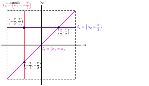
Figure 16: C-space of the degenerate 2-crank.

By gluing the sides, we obtain a torus with the embedded C-space formed by three circles

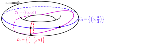
Figure 17: C-space of the degenerate 2-crank.

This example shows the difficulty of placing, counting, and computing DOFs in some none trivial examples. We see that $\alpha_{1}$ and $\alpha_{2}$ are both required to describe the system, even though the system has only one DOF. As we have seen, we have three cases:

1. If $\alpha_{1}$ is fixed, the freedom lies on $\alpha_{2}$.

2. If $\alpha_{2}$ is fixed, the freedom lies on $\alpha_{1}$.

3. If none is fixed, then $\alpha_{1}=\alpha_{2}$ and the freedom lies in both of them (although they are locked to each other).

It is interesting to note that this same issue might appear when trying to place gauge freedom (even for mechanical systems, see [10]) or boundary degrees of freedom in field theories (see [11]).

4 Conclusions

DOFs are one of the most important concepts taught in a first course in classical mechanics. They are also essential in other areas such as statistical mechanics, condensed matter, field theories and robotics. In this paper, we have tried to show that DOFs can be more subtle than one might expect, and some reflection needs to be done in order to gain a deeper knowledge and understanding. In particular, we have seen that one of the best ways to understand DOFs is as coordinates on the configuration space. As such, most of the time DOFs lack a physical meaning and cannot be located in a particular place. Of course, some choices can be made with direct physical correspondence (like angles or distances), but in general, it is not possible to choose our DOFs based on a physical representation of the system. The greatest benefit of this discussion is that this point of view also allows us to understand manifolds and topology better. Indeed, some surfaces with non-trivial topologies can be realized as mechanical systems as well as some higher dimensional manifolds. This approach provides an excellent motivation to a topology or differential geometry course for physicists.

References

- [1] Canadian Space Agency and NASA, Canadarm3: Canada’s smart robotic system for the Lunar Gateway, (2019).
- [2] K. Lynch and F. Park, Modern Robotics: Mechanics, Planning, and Control, Cambridge University Press (2017).
- [3] J. Marsden and T. Ratiu, Introduction to Mechanics and Symmetry: A Basic Exposition of Classical Mechanical Systems, Springer New York (1999).
- [4] T.W. Baumgarte and S.L. Shapiro, Numerical Relativity: Starting from Scratch, Cambridge University Press (2021).
- [5] T. Frankel, The Geometry of Physics: An Introduction, Cambridge University Press, 3 ed. (2011).
- [6] R.L. Brown, The klein bottle as an eggbeater, Mathematics Magazine 46 (1973) 244.
- [7] J.R. Munkres, Topology, vol. 2, Prentice Hall Upper Saddle River (2000).
- [8] W.P. Thurston and J.R. Weeks, The mathematics of three-dimensional manifolds, Scientific American 251 (1984) 108.
- [9] D. Jordan and M. Steiner, Compact surfaces as configuration spaces of mechanical linkages, Israel Journal of Mathematics 122 (2001) 175.
- [10] J. Prieto, E.J. Villaseñor et al., Gauge invariance in simple mechanical systems, European Journal of Physics 36 (2015) 055005.
- [11] B.A. Juárez-Aubry, J. Margalef-Bentabol, E.J. Villaseñor et al., Quantization of scalar fields coupled to point masses, Classical and Quantum Gravity 32 (2015) 245009.